
Abstract
With the fast development of unmanned aerial vehicles (UAVs) and the user increasing demand of UAV video transmission, UAV video service is widely used in dynamic searching and reconnoitering applications. Video transmissions not only consider the complexity and instability of 3D UAV network topology but also ensure reliable quality of service (QoS) in flying ad hoc networks (FANETs). We propose hedge transfer learning routing (HTLR) for dynamic searching and reconnoitering applications to address this problem. Compared with the previous transfer learning framework, HTRL has the following innovations. First, hedge principle is introduced into transfer learning. Online model is continuously trained on the basis of offline model, and their weight factors are adjusted in real-time by transfer learning, so as to adapt to the complex 3D FANETs. Secondly, distributed multi-hop link state scheme is used to estimate multi-hop link states in the whole network, thus enhancing the stability of transmission links. Among them, we propose the multiplication rule of multi-hop link states, which is a new idea to evaluate link states. Finally, we use packet delivery rate (PDR) and energy efficiency rate (EER) as two main evaluation metrics. In the same NS3 experimental scenario, the PDR of HTLR is at least 5.11% higher and the EER is at least 1.17 lower than compared protocols. Besides, we use Wilcoxon test to compare HTLR with the simplified version of HTLR without hedge transfer learning (N-HTLR). The results show that HTRL is superior to N-HTRL, effectively ensuring QoS.
1 Introduction
1.1 Research background
The explosive growth of network bandwidth has enabled the prosperity of videos in various fields. More and more fields are updating service contents, especially for video services. Nowadays, videos are reshaping the content of wireless services. Video transmissions generate a substantial fraction of the traffic on the network, and a reliable transmission network depends on a routing mechanism [4, 37]. In the past few years, the video service of unmanned aerial vehicles (UAVs) has obviously increased in dynamic searching and reconnoitering applications [6, 26], such as post-disaster searching, forest-fire spread sensing, tactical reconnaissance, intruder reconnoitering, and so on. UAVs could transmit video through flying ad hoc networks (FANETs) (also called flying self-organizing networks). For instance, UAVs search dynamic moving targets in the post-disaster searching scenarios. After the disaster, there are no available fixed communication infrastructures (e.g., 4G/5G infrastructures). Therefore, UAVs have to transmit the dubious target videos to the base station through FANETs. Then, users could judge whether these dubious target videos contain real moving targets in the base station. Driven by the continually updating demands from users, video transmissions through FANETs have become the essential service of dynamic searching and reconnoitering applications. Moreover, the multimedia routing required in video transmissions is also constantly developing.
The related works could be summarized as a research line from a multimedia routing perspective. In wireless multimedia sensor networks (WMSNs), stationary nodes are relatively easy to construct the shortest path and ensure QoS [2, 17, 28, 34]. However, energy-saving is an enormous obstacle to further improving their performances. In mobile ad-hoc networks (MANETs), the recent multimedia routing developments are mainly triggered by the robot technology progress and the growing robot applications [1, 5, 12, 29, 33, 38, 43, 51]. These researches focus on 2D application scenarios. In the past decade, FANET routing has been a research hotspot [3, 7, 11, 18, 23, 25, 36, 42, 49, 50]. However, the multimedia routing research for 3D multimedia FANETs is still in infancy [39, 41, 52]. In recent 5 or 6 years, the technological development demand of 3D multimedia FANETs is from the growing UAV applications. Generally, the new multimedia routing research is necessary to satisfy the emerging demand for 3D multimedia FANETs.
1.2 New challenges in 3D multimedia FANETs
To meet users’ demand for video services, 3D multimedia routing in self-organizing UAV networks still faces two major challenges [16]. And our research focuses on solving these two challenges of 3D multimedia FANETs. Two major challenges include:
-
The complexity and instability of 3D network topology. UAVs frequently reduce flight altitudes to capture dynamic moving targets or increase flight altitudes to expand the field of view in dynamic searching and reconnoitering applications. Due to introducing the flight-altitude axis, 3D network topology is more complex than 2D network topology. On the other hand, the speed of UAVs is unable to compare with the speed of ground vehicles. The speed of UAVs leads to the instability of 3D network topology. Thus, the complexity and instability of 3D network topology increase obviously in 3D multimedia FANETs.
-
The reliable Quality of Service (QoS) of video transmissions. Faced with 3D network topology, the reliable QoS is significant for video transmissions [35]. Packet delivery rate (PDR) is a necessary metric of QoS. Meanwhile, the energy efficiency performance of 3D multimedia FANETs is another essential metric because of the limited energies of UAVs.
1.3 Research method and our contributions
To address this research problem, we propose hedge transfer learning routing (HTLR) for dynamic searching and reconnoitering applications. A brief introduction to transfer learning is as follows.
-
Transfer learning background. As a new branch of machine learning, transfer learning is widely used in various fields [20, 22, 31, 32, 44, 45]. The basic idea of transfer learning is to transfer the knowledge learned in the source domain to different but related target domains [46]. This idea is consistent with human learning activities. For instance, a baby first learns how to distinguish their parents. Then, he could also use this existing ability to learn how to distinguish other persons.
-
Transfer learning practicality. In transfer learning, the transferred knowledge could be classified into models, features, relations, etc. Because transfer learning mainly uses the transfer procedure to exchange knowledge information, it has stronger practicality.
Therefore, we use hedge transfer learning as the kernel algorithm of HTLR. The contributions of the proposed HTLR include:
-
Hedge transfer learning. There are some communication applications of transfer learning [8, 9, 15, 27, 30, 46, 48], as shown in Table 1. Unlike these applications, we introduce hedge principle into transfer learning and propose hedge transfer learning. Due to using hedge principle, hedge transfer learning is robust to adjust the weight factors for online QoS-optimizing link state (QLS) and offline QLS models. Additionally, hedge transfer learning continuously updates these factors and online QLS model. As far as we know, there is little research on using hedge principle in transfer learning for communication applications.
-
Distributed multi-hop link-state estimation and its multiplication rule. As a distributed approach, multi-hop link-state values could estimate link states. UAVs choose the next-hop node to forward data packets based on the multi-hop link state. On the other hand, a multi-hop link consists of several single-hop links, and we approximately regard a multi-hop link state as the multiplication of several single-hop link states. This multiplication rule of multi-hop link states is a new idea to evaluate link states. Since this distributed estimation approach is based on broadcasting and timeout-period constraints, it will not be impacted by the dynamic topology of 3D multimedia FANETs.
-
Performance evaluation. Compared with four protocols in NS3 network simulator, HTLR outperforms others in terms of PDR and energy efficiency in most cases. The delay and jitter results of HTLR could be accepted when considering the real demand of dynamic searching and reconnoitering applications. To demonstrate the effectiveness of hedge transfer learning, we use Wilcoxon test (i.e., a non-parametric statistical test) to compare HTLR with the simplified version of HTLR without hedge transfer learning. The results of Wilcoxon test prove that hedge transfer learning effectively ensures QoS.
2 Related works
2.1 Multimedia routing
Existing multimedia routing research could be categorized by their focused networks, such as WMSNs, MANETs, FANETs, and so on. There are few kinds of research of 3D multimedia FANET routing protocols, as far as we know. It is still difficult to overcome the dynamic topology of 3D multimedia FANETs and perform reliable QoS multimedia transmission. Due to the emerging multimedia applications of UAVs, 3D multimedia FANET routing protocols are an important research direction.
2.1.1 Wireless multimedia sensor networks
As the earlier research, WMSNs fully investigate multimedia transmission to ensure QoS and improve energy efficiency. Adwan and Khaled review a large number of research works based on real-time QoS routing protocols for WMSNs [2]. Besides, Hamid and Hussain give an overview of the different existing layered and cross-layered schemes in WMSNs [17]. Nagalingayya and Mathpati study the maximum energy cooperative route in WMSNs. They introduce the recurrent neural network oriented decision-making system to select the appropriate cooperative nodes based on energy, reliability, and delay [34]. In addition to improving QoS and reducing energy consumption, the transmission security of WMSNs is also worth considering. To detect malicious nodes during data transmission, Kumar and Sivagami present a fuzzy logic system for calculating the trust score for each sensor node in the WMSNs [28]. And then, trust-aware routing is established between the source sensor and destination.
Different from MANETs and FANETs, nodes in WMSNs are usually stationary, while the network topology of WMSNs is static. Generally, these researches in WMSNs are the foundation for further research on multimedia data transmission in MANETs and FANETs.
2.1.2 Mobile ad hoc networks
Recently, unmanned ground vehicles and ground robot swarms have been widely used in various fields. This promotes the development of multimedia routing in MANETs. Different from the early-stage research of maximizing throughput in MANETs, how to establish QoS-guarantee multimedia transmission becomes popular. Adam and Hassan present an overview of reactive routing protocols for QoS and use the delay as a major metric [1].
Usually, QoS guarantee in multimedia MANETs is more difficult than WMSNs because of the mobility of nodes in MANETs. Multicast and multipath routing are widely studied because they can cope with network topology changes. Fleury et al. explain single-path and multi-path routing to ensure Quality of Experience (QoE) [12]. Masoudifar presents a global view and performance comparison of QoS multicast routing for MANETs [33]. Balachandra et al. consider a novel multiconstrained and multipath QoS aware routing protocol [5], which takes care of QoS parameters dynamically and simultaneously along with pathfinding. Thus, reliable and energy-efficient paths could be used for data transmission. Zhang et al. focus on improving the QoS and QoE in MANETs. They provide the QoE-driven multipath TCP-based data delivery model and present hidden Markov model-based optimal-start multipath routing [51]. Kumari and Sahana combine ACO, PSO, and a dynamic queue mechanism to improve QoS constraints and minimize data dropping [29]. Palacios Jara et al. guarantee QoS and the trust level between users who form the forwarding path in the MANETs by modifying the multipath multimedia dynamic source routing protocol [38]. Srinivasulu et al. present a QoS-aware energy-efficient multipath routing protocol and use the deep kronecker neural network to determine the optimum route [43]. However, multipath transmission transmits single-link data on multiple links, and the same data packet arrives at the base station. Although the transmission success rate is improved, energy consumption also increases. Moreover, multimedia routing protocols in MANETs mainly focus on 2D network scenarios and are not adaptive to 3D scenarios because 3D network topology is more complex than 2D network topology.
2.1.3 Flying ad hoc networks
Due to the developments of UAVs, multimedia routing protocols become more and more popular in FANETs. Jiang and Han present a comprehensive survey of various routing establishment protocols for FANETs [23]. There are three kinds of research that consider QoE/QoS guarantee.
2D application scenarios of FANETs. Recent studies focus on 2D application scenarios of FANETs. Souza et al. propose an adaptive routing protocol based on the fuzzy system for 200 m × 200 m area size [42]. And this multimedia routing protocol is assessed by QoS and QoE metrics, which is about 35% higher than AODV and OLSR. He et al. propose a utility function for the overall QoE and present an intelligent and distributed allocation mechanism to effectively solve the rate allocation problem of UAVs [18]. Considering QoE for FANETs, Arnaldo Filho et al. propose a relay placement mechanism (called MobiFANET) to establish the ideal relay location and show the effectiveness of MobiFANET that works jointly with a routing protocol [11]. Bhardwaj and Kaur propose a secure energy efficient dynamic routing protocol, aiming at maximizing the QoS standards and helping the nodes save their energy [7]. However, these 2D scenarios still cannot simulate real application scenarios. 3D network topology will bring greater challenges to routing.
3D UAV relay placement or location optimization. Recent studies also consider 3D UAV relay placement or location optimization to support downlink transmission. Jiang et al. study the proactive caching and UAV relaying techniques to maximize multimedia throughput in Internet-of-Things systems [25]. The UAV relay deployment is decomposed into vertical & horizontal dimensions, and the probabilistic caching placement is formulated as a concave problem. Niu et al. jointly optimize UAVs’ 3D location, power, and bandwidth allocation and meet the users’ requirements with different statistical delay-bound QoS in an emergency situation [36]. Zhang and Cheng derive the optimal power allocation scheme and introduce the statistical delay-bounded QoS provisioning framework, which could support diverse traffic in the UAV-enabled emergency network [49]. As base stations, UAVs are deployed for downlink transmissions, and device-to-device users operate in the underlying spectrum sharing mode. Considering cooperative UAVs for the downlink transmission of ground rescue vehicles in post-disaster areas, Zhang and Liu present a mathematical framework to analyze the coverage probability and average achievable rate for a multi-UAV-assisted downlink network, proving that the network performance gained [50]. Almeida et al. combine the placement of UAVs with a predictive and centralized routing protocol [3]. As a result, QoS provided to the users is improved.
The routing protocols of 3D multimedia FANETs. The routing protocols of 3D multimedia FANETs that consider 3D dynamic network topology and QoS/QoE guarantee are still in the infancy stage. Based on these challenges, the recent studies of 3D multimedia FANETs are reviewed as follows. Rosário et al. propose a link-quality and geographical-aware beaconless opportunistic routing protocol (named LINGO) for 40 m × 40 m area size [41]. Because LINGO focuses on link quality and geography information, it could be extended to 3D multimedia FANETs. Pimentel et al. propose an adaptive context-aware beaconless opportunistic routing (CABR) for 3D multimedia FANETs with QoE guarantee [39]. CABR comprehensively takes into account multiple types of context information to compute dynamic forwarding delay. Zhang et al. propose a three-dimensional Q-learning based routing protocol. The protocol predicts link status and makes routing decisions by using Q-learning to guarantee the packet delivery ratio and improve the QoS [52]. These studies mainly focus on link state, and the link quality is evaluated by location, delay, energy, and other metrics. This shows that QoS is closely related to link state in FANETs.
2.2 Transfer learning
2.2.1 Different application fields
As a new promising paradigm of machine learning, transfer learning has received close attention. In the past five years, there have been a few prominent solutions because of transfer learning practicality. Transfer learning has been successfully applied in medical treatment, image recognition, natural language processing, target detection, and other fields. Iskanderani et al. present a real-time IoT framework for the early COVID-19 diagnosis by using deep transfer learning, which could help radiologists diagnose suspected patients in COVID-19 efficiently [22]. To address the control problem of maneuvering target tracking and obstacle avoidance, Li et al. propose an online path planning method for UAVs based on deep reinforcement learning, which is supported by transfer learning to improve the generalization capability of UAV’s control model [31]. Lu and Lin study direct edge-to-edge cooperative transfer learning, which further improves the accuracy of image recognition [32]. In general, it could be seen that most transfer learning research focuses on image processing, signal analysis, and medical care [20, 44, 45].
2.2.2 Present applications in communication
Due to the success of transfer learning in many fields, there is emerging research on transfer learning and communication. Moreover, these interdisciplinary researches are meaningful, which gradually increases as a new research hotspot. Generally, the flexibility and practicability of transfer learning are the better-performance root of these problems.
Besides, the application of transfer learning in communication is summarized in Table 1. There is little research on transfer learning in the routing protocols of MANETs and FANETs to our best knowledge. The present applications of transfer learning in communication include:
-
Advances and challenges of transfer learning in promoting wireless communication. Wang et al. present a comprehensive review of transfer learning used in different wireless communication fields and discuss the future research directions between transfer learning and 6G communications [46].
-
Energy saving in cellular radio access networks. Li et al. propose transfer actor-critic algorithm (TACT) that uses the transferred learning knowledge & reinforcement learning [30]. And they prove the convergence of TACT.
-
Interference mitigation in 5G millimeter-Wave communications. Elsayed et al. propose transfer Q-learning (TQL), Q-learning, and best SINR association with density-based spatial clustering of applications with noise algorithms [9]. TQL outperforms others in both mobile and stationary application scenarios.
-
Traffic engineering in experience-driven networking. Xu et al. propose an actor-critic-based transfer learning framework (ACT-TE) to solve the traffic engineering problem [48]. ACT-TE significantly outperforms straightforward & traditional methods in terms of network utility, throughput, and delay.
-
Dynamic routing in software defined networking. Dong et al. propose a transfer reinforcement learning (TRL) algorithm to improve the training efficiency and deal with the changes of network state and topology [8]. TRL has high training efficiency and outperforms deep reinforcement learning-based routing frameworks.
-
Classical frameworks of transfer learning in cellular radio access networks and 5G new radio mmWave networks. Konda and Tsitsiklis propose a class of actor-critic algorithms for simulation-based optimization of a Markov decision process [27], which is characterized by actor-critic framework. Besides, Grondman et al. present a detailed survey for several standard and natural actor-critic algorithms [15]. Their focus is an online setting and using function approximation to deal with continuous state and action spaces.

3 Network model
3.1 Assumptions
3.1.1 Location and speed
UAVs are equipped with GPSs and altitude gauges. Through these devices, they could obtain their 3D locations and speeds.
3.1.2 Mobility model
NS3 is a network simulator commonly used for MANETs’ and FANETs’ simulations. In dynamic searching and reconnoitering applications, UAVs fly randomly according to task positions in 3D space, and the base station does not move around on the ground. Therefore, in our simulations, we use the 3D random waypoint model of NS3 as the mobility model of UAVs. In this mobility model, UAVs exist in the form of nodes. Besides, we assume that the base station in NS3 is fixed at the center of the simulation area. We explain the 3D random waypoint model of NS3 as follows.
-
Movement procedure. The node moves forward to the task position at a fixed speed. When the node reaches the task position, it does not stop for a while. This node selects a new random destination, uses a new random speed, and continues to move.
-
Speed change. When each node reaches its destination, then it will select a new random speed. The speed of each node changes from the minimum value (i.e., the setting parameter) to the maximum value (i.e., another setting parameter). We use the average value of the minimum and the maximum values to express the actual speed of each node for different simulation results in this paper.
3.1.3 Device and energy
UAVs are homogeneous in respect of hardware. Due to UAV mobility, they have limited energy. Besides, the base station is located on the ground, which has unlimited energy. We use the simple radio energy dissipation model [19] as the energy consumption model for UAVs and the base station. The free space or multipath fading channel model is selected according to the distance between the sending and receiving nodes. Moreover, the energy consumption of radio hardware is considered. The transmitter energy consumption Etx and receiver energy consumption Erx of the model are given by
where k is the number of bits and Eelec is the consumed energy for receiving or sending a bit. d is the distance from the transmitter to the receiver. As a distance threshold, d0 is equal to (εfs/εmp)0.5. If d ≤ d0, it uses the free space channel for calculation; Otherwise, it uses the multipath fading channel. εfs and εmp are the amplification coefficients for the free space and multipath fading channel models, respectively.
3.1.4 Multimedia transmission
UAVs search and reconnoiter dynamic moving targets, while simultaneously transmitting videos to the base station. Considering the actual scenarios of dynamic searching and reconnoitering applications, we assume that there are 10% UAVs as video sources in the multimedia transmission period.
3.2 Communication links
3.2.1 Air-to-air links among UAVs
UAVs use three-dimensional omnidirectional antennas to expand the communication range. In other words, the links among UAVs are bidirectional. If UAV A could send data packets to UAV B, UAV B could also transmit data packets to UAV A. The communication boundary of each UAV is a sphere centered on itself in the air.
3.2.2 Air-to-ground links between UAVs and base station
Air-to-ground links between UAVs and the base station are in accord with actual communication links, which are constrained by communication radius and UAV height. UAVs form a cone to mark the communication regions on the ground.
4 Hedge transfer learning routing
Transfer learning has strong applicability and can cope with the complexity and instability of 3D network topology. In addition, the introduction of hedge principle could enhance the robustness of transfer learning. To ensure PDR and energy efficiency, HTLR uses hedge transfer learning and the multi-hop link scheme to fight against the topology changes of 3D multimedia FANETs.
4.1 Hedge transfer learning
Different from TACT [30], TQL [9], ACT-TE [48], and TRL [8], the hedge framework of hedge transfer learning is based on hedge principle. In general, hedge principle is the cornerstone to support the operation of this online learning. Moreover, we discuss the rationality of hedge principle in Section 4.1.1.2.
In this paper, hedge transfer learning belongs to model-based transfer learning. It is worth noting that the real-time performance of HTLR is only related to the online parts of hedge transfer learning in Sections 4.1.1.2 and 4.1.4, which could satisfy the practicability requirement of HTLR.
4.1.1 Online learning in the base station
When UAV transmits video, the 3D network topology of FANETs is always changing. However, in the adjacent time periods, the transmission features of 3D multimedia FANETs are similar to each other, such as nine input parameters (x1, x2, ..., x9) in Section 4.1.2. Therefore, based on the transmission-feature similarity in the adjacent time periods, online learning is chosen to improve the adaptability of hedge transfer learning to 3D dynamic topology of FANETs.
Hedge framework
As shown in Fig. 2, the base station runs hedge transfer learning that includes:
-
Offline domain. Offline domain is the source domain of transfer learning [46]. As shown in Section 4.1.3, offline domain consists of offline data collection, offline large-scale dataset, and offline training. The output of offline domain is offline QLS model.
-
Online domain. Online domain is the task domain of transfer learning [46]. As shown in Section 4.1.4, online domain consists of online data collection, online small-scale dataset, and online training. The input of online domain is transferred QLS model from offline domain, which is used to initialize online QLS model. And the output of online domain is online QLS model. The real-time requirements of HTLR are different for offline with online domains. Offline domain need not consider the real-time requirement of HTLR. On the contrary, online domain should satisfy the real-time requirement of HTLR. Therefore, this paper uses both offline domain and online domain. Moreover, offline domain and online domain are independent to each other.
-
Hedge transfer learning. Hedge transfer learning adjusts online and offline weight factors Fon and Foff for online and offline QLS models. It is worth noting that·the collected online data are continuously updated to adapt to the dynamic topology of networks. Then, online QLS model, Foff, and Fon are also constantly adjusted.

Online learning in the base station
Hedge principle
UAVs apply online QLS model, Fon, and Foff to build single-hop link state scheme in Fig. 3. It is worth noting that online QLS model, Fon, and Foff in Fig. 2 are continuously updated by using broadcasting packets from the base station. And offline QLS model is fixed to the program memory of UAVs in advance. These will be explained in Section 4.2.

Applying online QLS model, Fon, and Foff to single-hop link state scheme in UAVs
Hedge transfer learning to obtain Fon and Foff. Hedge transfer learning procedure is based on hedge principle to adjust Fon and Foff [13]. Algorithm 1 depicts the procedure of hedge transfer learning. As the main part of Algorithm 1, hedge principle corresponds to lines 6 ~ 15. Hedge principle means that the better QLS model (offline or online QLS model) will have a relatively greater contribution to single-hop link state. For each item of online data, the update strategy of Fon and Foff is given in Eqs. 4–7. The explanations are as follows.
-
Determine the decay degree. Ψ(x) is the loss function with decay factor β to determine the decay degree. The output-value errors of offline and online QLS models are |Y1-Q1| and |Y1-Q2|. Then, loss values are Ψ(|Y1-Q1|) and Ψ(|Y1-Q2|). Greater error, greater loss value Ψ(x), and greater decay.
-
Update weight factors. After obtaining these decay values, it uses multiplication to update weight factors in Eqs. 4 and 5. That is, it penalizes the weight factors this time.
-
Normalized weight factors. Redistribute two weight factors through normalization in Eqs. 6 and 7. This shows that we give more weight to models that perform better.

The procedure of hedge transfer learning to obtain Fon and Foff
The reliability of hedge principle to adjust Fon and Foff. Due to robustness, hedge principle is widely used in different fields, such as hedge funds. In this paper, hedge principle could adjust Fon and Foff in a reliable mode. Offline and online QLS models are regarded as two experts in hedge principle. Offline QLS model trained by using a large number of data items is a common-skill expert, while online QLS model is a special skill expert that continuously learns from the present small-scale network data. When evaluating single-hop link states, we ask two experts for their advice. Moreover, our goal is to combine this advice so that the expected losses are not much worse than the best expert. We define the contribution weights Fon and Foff of two experts to realize this goal. Then, we do the procedure of hedge transfer learning in Algorithm 1. Through this reliable hedge procedure, single-hop link state is flexible enough to maintain a satisfactory evaluating-link capability in the entire network lifecycle.
The computational complexity of hedging transfer learning. The computational complexity of hedge transfer learning is critical to the real-time performance of HTLR. Algorithm 1 includes initialization and hedge procedure. The computational complexity of initialization is O(3) + O(2) + O(9 × Nd), and the computational complexity of hedge procedure is O(3 × Nd) + O(3 × Nd) + O(2 × Nd). Thus, the computational complexity of Algorithm 1 is approximately equal to O(Nd). This means that the computational complexity of Algorithm 1 depends on the data-item number of online small-scale dataset Nd. When Nd = Nmax = 6000, the running time of hedge transfer learning once is about 0.013 seconds in Linux system with Intel (R) Xeon (R) CPU ×5670 @ 2.93GHz and 128G memory. Because the running time of hedge transfer learning once (i.e., 0.013 seconds) is much less than transfer period (transfer period = 20s), the procedure of hedging transfer learning could satisfy the real-time requirement of HTLR.
4.1.2 QLS model
From a QoS perspective, QLS model is defined to evaluate link states. The dynamicity of 3D multimedia FANETs is complicated over time. Therefore, to make QLS model more flexible, we choose artificial neural network as our QLS model. We train offline and online QLS models by using offline and online data.
Structure
The structure of QLS model includes one input layer with nine neurons, three hidden layers with nine neurons, and one output layer with one neuron. Based on the multi-layer structure, QLS model could provide the flexible functionality to choose a rational next-hop data-forwarding UAV. Besides, the activation function is sigmoid, and the learning rate is 0.5.
Input parameters
Nine input parameters (x1, x2, ..., x9) are defined, focusing on network mobility and multimedia transmission features. These inputs translate mobility scenarios and multimedia transmission requirements into the following formulas.
Three mobility inputs (x1, x2, x3) could mirror the UAV-neighbor topology changes. These mobility inputs pay attention to the relative positions and speeds of transmitting UAVs, neighbor UAVs, and the base station. x1, x2, and x3 are given by
where Dsd is the present distance between the transmitting-UAV position and the predicted base-station position, Ps is the present position of transmitting UAV from GPS. Pd is the predicted base station position. R is the communication radius in Eq. 8. Dfw is the forward distance. Dnd is the present distance between the predicted neighbor-UAV position and the predicted base-station position in Eq. 9. \({\overrightarrow{V}}_{re}\) is the relative speed between UAV and neighbor UAV. \({\overrightarrow{V}}_s\) and \({\overrightarrow{V}}_n\) are the speeds of transmitting and neighbor UAVs. Vmax is the normalized maximum speed in Eq. 10.
Six multimedia transmission inputs (x4, ..., x9) with low computation costs are considered, which are given by
where Tthr is a cut-off delay threshold that is equal to 50 ms in this paper. Ts is the single-hop delay for neighbor UAVs in Eq. 11. Cd is the congestion degree in one period. Cfw is the count of forwarding packets. Cmax is the normalized maximum count, which corresponds to the length of one period in Eq. 12. Qr is the size of the remaining buffer queue. Qmax is the maximum length of buffer queue in Eq. 13. Nfr is the number of forward nodes that are close to the base station. Nbw is the number of backward nodes that are far from base station. Nmax is the normalized maximum number of nodes in Eq. 14 and Eq. 15. Er is the residual energy of each neighbor UAV. Emax is the initial energy of UAVs in Eq. 16.
Output parameters
We abstract three key parameters: forward distance Dfw, energy consumption Ec in one period, and single-hop delay Ts. These parameters are formulated as the output Y1(x1, ..., x9) of QLS model. Y1(x1, ..., x9) is given by
where q1, q2, and q3 are three components. Tthr is a cut-off delay threshold, and Emax is the initial energy of UAVs. When collecting offline or online data (x1, ..., x9) and (q1, q2, q3) are also collected. For each UAV, if the transmission of data packet is failed, then Y1(x1, ..., x9) = 0. This means that this neighbor UAV should not be chosen to forward data packets. Otherwise, this neighbor UAV could be chosen.
In this paper, we use PDR and energy efficiency as QoS metrics. These QoS metrics are realized by the weights of q1 and q2 being greater than that of q3, as shown in Eq. 17. Greater Y1(x1, ..., x9) value means a greater probability to ensure QoS. According to different Y1(x1, ..., x9) values for neighborhood UAVs, transmitting UAVs could distinguish available neighborhood UAVs from unavailable neighborhood UAVs. To further explain Y1(x1, ..., x9), the principle discussions of q1, q2, and q3 are as follows.
-
q1 uses the forward distance Dfw to a single-hop UAV neighbor. This means shortening the distance between the present data-packet position and the base station. Generally speaking, shorter Dfw means closer to the base station and a higher probability of successful transmission. Thus, q1 corresponds to improving PDR.
-
q2 is defined by using the energy consumption of the neighbor UAV in one period. With q1 guaranteed, choosing a UAV with less energy consumption is effective in balancing the energy consumption of UAVs in the neighborhood. Smaller Ec means better energy efficiency in most cases. Thus, q2 corresponds to energy efficiency.
-
q3 expresses the delay of a single-hop link, which is used to improve the delay performance of HTLR.
Discussions
In HTLR, the input and output parameters of QLS model (x1, ..., x9, q1, q2, q3) are inserted into data packets. In practice, the base station could collect these parameters through data packets. This means that QLS model could be used in practice. The specific analysis is as follows.
-
How to obtain the input parameters of QLS model in practice? UAVs are equipped with GPSs and altitude gauges for three mobility inputs (x1, x2, x3), which insert these mobility inputs into data packets. When the base station receives data packets, it unpacks data packets to obtain these input parameters. Besides, six multimedia transmission inputs (x4, ..., x9) could also be obtained by using this approach.
-
How to obtain the output parameters of QLS model in practice? The collection procedure of three output parameters (q1, q2, q3) is similar to input parameters.
4.1.3 Offline training for offline QLS model
Offline training time. Offline QLS model is trained by using offline large-scale dataset. Because training offline large-scale dataset does not need to occupy online time, the offline-QLS-model training time does not affect the online running time of HTLR. The training time of offline QLS model is 16.07 seconds in Linux system with Intel (R) Xeon (R) CPU ×5670 @ 2.93GHz and 128G memory.
Offline data collection. We collect offline large-scale dataset in NS3 network simulator. In our simulation, 3D space size is 1000 m × 1000 m × 1000 m, mobility model is 3D random waypoint mobility, node speed randomly changes from 0 m/s to 50 m/s, and base station is located in the center of the ground. In this paper, 20,000 items of offline training data have been collected.
Offline training procedure. The training method of offline QLS model is RProp [40]. RProp does not consider the magnitude of the gradient. It only determines the adjustment direction of the connection strength in terms of the direction of the gradient. The same learning abilities in each layer are not affected by the distance from it to the output layer. This computation process is simple. Therefore, it could quicken the converging speed and overcome the local minimum problem. In terms of offline training parameters, the maximum number of training iterations is 500, and the expected error is 0.005. The stop condition of offline training is that the present number of training iterations is 500 or the training error is less than the expected error.
4.1.4 Online training for online QLS model
The offline QLS model under offline training could not cope with the real-time changes of 3D network topology, so the online QLS model under online training is introduced. The details of online training time, data collection and training procedure are as follows.
Online training time. In the base station, online QLS model is trained by using online small-scale dataset. As online learning algorithms, the training and running times of online QLS model are critical to the real-time performance of HTLR. The training time of online QLS model for online small-scale dataset is short. In this paper, the training and running times of online QLS model is about 2.55 seconds and 4.67e-6 seconds in Linux system with Intel (R) Xeon (R) CPU ×5670 @ 2.93GHz and 128G memory. These times are much less than transfer period (transfer period = 20s).
Online data collection. HTLR uses base station to collect online data and realize online training. Online data are collected by the base station from the real-running simulation of HTLR. These data include the training data of successful transmission and the training data of failure transmission in the last transmission. It is worth noting that UAVs add this failure-transmission information to the present data packet. If the base station receives this packet, it could unpack the failure-transmission information as online training data.
Online training procedure and its computational complexity. Algorithm 2 demonstrates how to train online QLS model by using RProp and online small-scale data. After calculating the pseudo-code of RProp, the computational complexity of RProp is O(Nd) (Nd is online data and its item number). Therefore, the computational complexity of Algorithm 2 is O(Nd). Specifically, there are two start and one stop conditions of online training as follows.
-
The first start condition. The time interval from the last training time to the present time exceeds transfer period. Moreover, the number of online training data items is greater than or equal to the minimum number of online training data items Nmin (Nmin = 4000).
-
The second start condition. The number of online training data items is greater than or equal to the maximum number of online training data items Nmax (Nmax = 6000).
-
The stop condition. Due to the small size of online data items, the maximum number of training iterations is set to 200, and the expected error is 0.001. This could ensure generalization ability and the training time of online QLS model.
Online training enables HTLR to better adapt to topology changes. Although the network topology is dynamic, this approximately periodic training could reflect the present network changes. Moreover, as a continuous updating component of HTLR, the output value of online QLS model is more suitable to evaluate the present links.

Training online QLS model by using online data
4.1.5 Differences and limitations
Compared with other transfer learning algorithms, the differences and limitations of hedge transfer learning include:
-
On research problem. We focus on 3D multimedia FANETs, which is different from the focused communication networks of [8, 9, 30, 48].
-
On transfer learning frameworks. Compared with TACT [30], TQL [9], ACT-TE [48], and TRL [8], hedge framework does not use the actor-critic algorithm, Q-learning, and reinforcement learning. This is a difference between hedge framework and these union frameworks [8, 9, 30, 48], as shown in Figs. 1 and 2. There is little research that uses hedge principle in transfer learning, as far as we know.
-
On advantages. Hedging transfer learning has better sensitiveness and robustness.
-
The online data sensitiveness is able to ensure mirroring time-varying network states. Online data that base station collects is changing with time-varying network states. Moreover, online data are sensitive to the changes of network states, such as available residual-link-communication time. For instance, if the speeds of UAVs increase, then available residual-link-communication time decreases. At this moment, the collected online data could record what kinds of links are more suitable for transmitting data packets. In other words, the collected online data could record the speed-increase influence on all communication links. Then, when training online QLS model, these online data with the present network states could strengthen the online-QLS-model capability for the speed increase of UAVs.
-
Combining offline large-scale dataset training with online small-scale dataset training improves the robustness. Offline QLS model is trained by using offline large-scale dataset. Due to the large size of offline data items, offline QLS model usually has better adaptability for various network scenarios. However, offline QLS model does not combine with the present online-target network states. Online small-scale dataset could mirror the present online-target network states used to train online QLS model. Based on the online data beforehand calibration and hedge principle, Fon and Foff are adjusted dynamically over time.
-
-
On limitations. Hedge transfer learning has some limitations. Due to hedge framework, online and offline QLS models must be homogeneous.
4.2 Routing procedure
The routing procedure includes two parts: transfer routing and data forwarding.
4.2.1 Transfer routing
The objective of transfer routing is to transmit online QLS model, Fon, and Foff from the base station to UAVs, as shown in Fig. 4. Detailed explanations of transfer routing are as follows.
-
The left side of Fig. 4 shows the operation procedure of the base station, such as running hedge transfer learning and broadcasting online QLS model, Fon, and Foff to UAVs. The contents of broadcast packages could be obtained from Section 4.1.1.2. If UAVs receive these broadcasting packets, they will update their corresponding parameters and continue to broadcast. In most cases, all UAVs could receive these broadcasting packets. It is worth noting that offline QLS model is fixed to the program memory of UAVs in advance. This also means that the base station is not required to transmit offline QLS model to UAVs.
-
The right side of Fig. 4 gives the procedure of data forwarding. It also explains the relationship between multi-hop link state and data forwarding.
Fig. 4 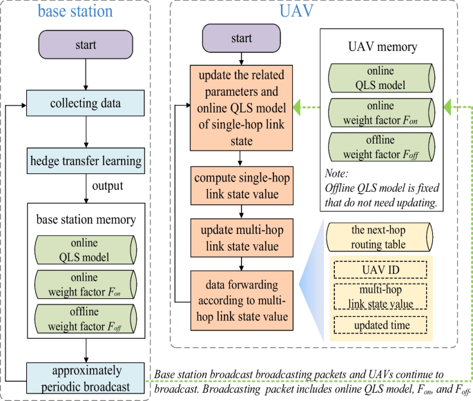
The transfer routing procedure of HTLR

4.2.2 Data forwarding
Because data forwarding procedure determines how to choose the next-hop data forwarding node, this is the kernel routing part of HTLR.
Algorithm 3 explains the routing procedure that UAVs forward data packets, such as timeout updating, early-warning updating, choosing a neighbor UAV as the next-hop forward node, and so on. When each transmitting UAV chooses data forwarding node from its neighbor UAVs, it will select the unexpired & unwarned neighbor with the maximum value of multi-hop link state as the next-hop data forwarding node. Discussions for Algorithm 3 are as follows.
-
The computational complexity of data forwarding procedure. The computational complexity of Algorithm 3 is mainly in cycling through the NHR table. The computational complexity of traversing the NHR table is O(NNHR) (NNHR is the number of UAV IDs in the NHR table).
-
A limit of HTLR. To improve PDR, HTLR takes advantage of the timeout period and early warning UAV-ID list to avoid using the unstable links in Algorithm 3. However, this may lead to the failure of data forwarding in some cases. For example, one UAV has fewer neighbor UAVs.

Data forwarding procedure
Focusing on multi-hop link states, Fig. 5 explains the routing design of data forwarding. For instance, the multi-hop link state of UAV B is greater than the multi-hop link state of UAV C (i.e., MLSB > MLSC). This means the multi-hop links of UAV B have a greater probability of successfully transmitting data packets than the multi-hop links of UAV C. Therefore, UAV A compares MLSB with MLSC in its next-hop routing table. Due to MLSB > MLSC, UAV A chooses UAV B as the next-hop forward node. Similarly, the link state of base station is greater than the multi-hop link state of UAV D (i.e., MLSBS > MLSD), and MLSBS is always equal to 1 in this paper. Because of MLSBS > MLSD in the next-hop routing table of UAV B, UAV B directly forwards data packet to base station.

The example of data forwarding through multi-hop link state
Next, multi-hop link state that is the key point of data forwarding, and we explain this key point as follows. Multi-hop link state scheme is a distributed approach to estimate multi-hop link states. Because single-hop link state scheme in Section 0 is the basis of multi-hop link state scheme in Section 4.2.2.2. Thus, we first introduce the single-hop link state scheme in Section 4.2.2.1 and then present the multi-hop link state scheme in Section 4.2.2.2.
Single-hop link state scheme
Single-hop link state scheme could evaluate the single-hop link states of neighbor UAVs, which includes online QLS model, Fon, offline QLS model, and Foff. In the single-hop link state scheme, offline QLS model is fixed in the program memory of each UAV beforehand. Besides, online QLS model, Fon, and Foff are continuously updated from received broadcasting packets.
The input and output of single-hop link state. In the routing procedure, the input of the single-hop link state scheme is the present input (x1, ..., x9), as shown in Fig. 3. These present inputs are the real-time information that is obtained from neighbor UAV broadcasting information. The single-hop link state value could express the probability of successfully forwarding data packets to this neighbor UAV. The output value of single-hop link state is from 0 to 1. From a single-hop perspective, greater single-hop link state, better capability to ensure QoS. Transmitting UAV could compute single-hop link states of neighbor UAV links. The output of single-hop link state SLS(A → B) is given by
where SLS(A → B) represents the function of transmitting data packet from UAV A to UAV B, which returns the probability of successfully forwarding data packets to UAV B. SY1(x1, ..., x9) and DY1(x1, ..., x9) are the outputs of offline and online QLS models.
An example of single-hop link state. For instance, when UAV A receives the broadcasted information of its neighbor UAV B, UAV A could obtain 9 input parameters (x1, ..., x9) of UAV B. According to this information, UAV A could obtain SY1(x1, ..., x9) and DY1(x1, ..., x9) for the single-hop link between UAV A and its neighbor UAV B. UAV A uses Eq. 19 and obtains the single-hop link state SLS(UAV A → UAV B). Similarly, based on the broadcasted information of neighbor UAVs, UAV A could obtain all single-hop link states between UAV A and neighbor UAVs.
Multi-hop link state scheme
Multi-hop link state scheme could evaluate the multi-hop link states from transmitting UAV to base station. This scheme is a distributed approach of updating multi-hop link state value.
The meaning of multi-hop link state and its computational complexity. From a multi-hop perspective, greater multi-hop link state value, greater probability of successfully transmitting data packets to base station. Each UAV has its own multi-hop link state value that is proportional to its best QoS capability to transmit data packets. Algorithm 4 gives the procedure of updating multi-hop link state. Because Algorithm 4 is only a process of constantly judging and updating, its computational complexity is very low. Thus, we needn’t consider its computational complexity.

The procedure of updating multi-hop link state
Mathematically, we define multi-hop link state by using multiplication and maximum-value rules. Meanwhile, each UAV uses the maximum value of multi-hop link states as its multi-hop link state value. Figures 6 and 7 further explain these rules of multi-hop link state as follows.
Multiplication rule. The multi-hop link state of each UAV could be approximately regarded as the multiplication factor of several single-hop link states. Generally speaking, multi-hop links consist of several single-hop links. Due to multiplication rule, the poor single-hop links with the low single-hop link state values will greatly decrease the multi-hop link state value. Therefore, multiplication rule is a reasonable choice to avoid choosing multi-hop links with poor single-hop links. By choosing these better multi-hop links, UAVs could improve PDR. To simplify the problem, we suppose that there are only base station, UAV A, and UAV B. Figure 6 gives this simplest example: two-hop links from base station to UAV A and from UAV A to UAV B. Through the broadcasting information of base station, UAV A could obtain the single-hop link state from base station to UAV A by using Eq. 19. Because base station only receives data packets and does not need forwarding data packets, the multi-hop link state value of base station (i.e., MLSBS) is always equal to 1. Then, UAV A could compute its multi-hop link state MLSA by using Eq. 20. Similarly, UAV B could obtain its multi-hop link state MLSB by using Eq. 21.
where SLS(base station→UAV A) is the single-hop link state from base station to UAV A. SLS(UAV A → UAV B) is the single-hop link state from UAV A to UAV B. This multiplication rule is a new idea to evaluate link states.

An example to demonstrate the multiplication rule of multi-hop link state scheme
Maximum-value rule. Each UAV uses the maximum value of the multi-hop link states of all neighbor-UAV links as its multi-hop link state. Because the single-hop link state value is from 0 to 1, the multi-hop link state is also from 0 to 1 through Eq. 21. According to the multiplication-rule meaning, the maximum value of multi-hop link states of all neighbor-UAV links means the best multi-hop link state to ensure QoS. To simplify the problem, we suppose that there are only UAV B, UAV C, and UAV D in the neighbor of UAV A. Figure 7 gives this star-topology example. UAV A could receive three values of multi-hop link states from UAV B, UAV C, and UAV D. Then, UAV A could also obtain three values of single-hop link states for three links (i.e., SLS(UAV B → UAV A), SLS(UAV C → UAV A), and SLS(UAV D → UAV A)) by using Eq. 19. For this star-topology situation, UAV A could obtain its multi-hop link state MLSA by using
where max() returns the maximum value.

An example to demonstrate the maximum-value rule of multi-hop link state scheme
4.2.3 Computational complexity
Base station program
The base station runs Algorithm 1 to perform hedge transfer learning, and the computational complexity of Algorithm 1 is O(Nd) (Nd is the data-item number of online small-scale dataset). For details, please refer to the last paragraph of Section 4.1.1.2. The base station runs Algorithm 2 to train the online QLS model, and the computational complexity of Algorithm 2 is O(Nd). For details, please refer to the fourth paragraph of Section 4.1.4. Therefore, the computational complexity of base station program is O(Nd) + O(Nd), which is approximately O(Nd).
UAV node program
UAV node runs Algorithm 3 to forward data, and the computational complexity of Algorithm 3 is O(NNHR) (NNHR is the number of UAV IDs in the NHR table). For details, please refer to the third paragraph of Section 4.2.2. UAV node runs Algorithm 4 to update multi-hop link state, and the computational complexity of Algorithm 4 need not be considered. For details, please refer to the second paragraph of Section 4.2.2.2. Therefore, the computational complexity of UAV node program is O(NNHR).
5 Simulation results and discussions
Compared protocols and experimental objectives
To demonstrate the performance of HTLR and the effectiveness of hedge transfer learning, GPSR_3D [14], SP_GMRF [21], GGFGD [24], 3DPBARP [10], and N-HTLR are used as compared protocols. Five compared protocols are divided into two groups:
-
The first group to demonstrate the performance of HTLR. The first group includes GPSR_3D, SP_GMRF, GGFGD, and 3DPBARP. (1) GPSR_3D is an extended routing protocol of greedy perimeter stateless routing algorithm (GPSR) in three-dimensional space, including two packet forwarding modes of greedy forwarding mode and surface forwarding mode, with high reliability, energy saving, and storage efficiency. (2) SP_GMRF is a 3D multicast geographic routing protocol for FANETs, which improves the scalability when nodes move frequently by using local information to construct a group multicast routing tree structure. (3) GGFGD is a geographic multipath routing for 3D underwater wireless sensor networks based on geospatial division. In GGFGD, a greedy geo-forwarding multipath strategy based on geospatial division is proposed by considering the characteristics of 3D topology and propagation delay. (4) 3DPBARP is a geographical 3D position-based routing protocol with mobility prediction. It adds a stable decision considering node mobility, while simultaneously using the change of geographical information, direction, and speed to determine the node’s transmissions.
-
The second group to demonstrate the effectiveness of hedge transfer learning. The second group includes N-HTLR. N-HTLR is a simplified version of HTLR without hedge transfer learning. In other words, the single-hop link state scheme in N-HTLR only uses offline QLS model and Foff = 1, which does not include online QLS model, Fon, and the procedure of hedge transfer learning in Algorithm 1.
Parameter setting
We program five compared protocols and HTLR by using C/C++ in NS3 network simulator. The network parameters setting is shown in Table 2. We set the data transmission rate as 320 kbps, which belongs to the multimedia transmission rate range [47]. Besides, we set UAVs to send videos to the base station every 10 seconds, and the period of multimedia transmission is 10 seconds in this paper. Each run of our simulations uses the newly generated mobility scenario to evaluate these protocols.
Evaluation metrics
Except for PDR, delay, and jitter, we define the energy efficiency ratio EER as an energy-saving criterion in Eq. 23. Lower EER, better energy-saving performance. UAVs’ energy consumption includes the energy consumption of sending data packets, receiving data packets, and broadcasting in the simulation. We set PDR and EER as the evaluation metrics of QoS. The higher PDR and lower EER mean the better QoS.
5.1 Comparison of general performance
3D multimedia routing protocols should consider PDR, EER, delay, and jitter to ensure multimedia QoS transmissions. To test these general performances of HTLR, the first group of compared protocols is used. Figure 8 presents the general results when node number = 100, the average speed of node = 25 m/s, and simulation time = 50 ~ 400 s. The explanations are as follows.
-
Figure 8(a) shows the variation trend of PDR with the increase of simulation time. HTLR has better PDR than others. For instance, the PDR gap between HTLR and SP_GMRF is approximately 6%. This indicates that data forwarding is effective through multi-hop link states in HTLR. Besides, this also means that hedge transfer learning could correctly adjust online QLS model, Fon, and Foff. Moreover, these results could demonstrate that hedge transfer learning is robust in most cases.
-
Figure 8(b) shows the variation trend of EER with the increase of simulation time. The EER result of HTLR is the best in all protocols. Lower EER means better performance of saving energy. When simultaneously considering PDR and EER for the first group and HTLR, the comprehensive performance of PDR and EER for HTLR is also the best. This means that HTLR realizes our objective of ensuring the PDR and EER metrics.
-
Figure 8(c) and (d) provide the results of delay and jitter change with the increase of simulation time. Naturally, HTLR is not good enough. From a delay perspective, HTLR is about the third best. From a jitter perspective, HTLR is about the second or third best. The reason is that HTLR must use more hops to improve PDR. Thus, more hops mean longer delay and more unstable jitter in most cases.
Generally, HTLR improves PDR and reduces EER even when facing the complexity and instability of 3D network topology. In 3D multimedia FANETs, PDR and EER are more important than delay and jitter for dynamic searching and reconnoitering applications. Moreover, these delay and jitter results could be acceptable in most searching and reconnoitering applications.

The general comparison when node number = 100, the average speed of node = 25 m/s, and simulation time = 50 ~ 400 s. a Packet delivery rate. b Energy efficiency ratio. c Delay. d Jitter
5.2 Effect of network mobility
More links become unstable due to network mobility. Therefore, it is necessary to test the practicality of HTLR for different node-speed scenarios. Besides, compared with the first group of compared protocols, it is also compared with the second group (i.e., N-HTLR) to demonstrate the effectiveness of hedge transfer learning. Figure 9 presents the results when node number = 100, the average speed of node = 10 ~ 40 m/s, and simulation time = 200 s. Details are as follows.
-
With the average speed of node increasing in Fig. 9(a) and (b), HTLR outperforms the first group in terms of PDR and EER. Moreover, with the average speed of node increasing, the advantage of HTLR is more obvious.
-
Comparing the average speed of node = 40 m/s with the average speed of node = 10 m/s, the gap between other protocols and HTLR gradually becomes great. Thus, we could conclude that the multi-hop link state scheme accurately estimates the time-varying link states. Meanwhile, this also indicates that deleting the expired links from the next-hop routing table is effective in improving the probability of successfully choosing forwarding nodes.
-
Compared with N-HTLR, hedge transfer learning could improve the PDR results of HTLR 2.67% ~ 4.18% and reduce the EER results of HTLR 0.39 ~ 5.97. Moreover, these two trends are always stable in the whole node-speed-change range.
-
-
With the average speed of node increasing in Fig. 9(c) and (d), the delay and jitter results of HTLR are still not good enough. However, with the average speed of node increasing, the delay and jitter results of HTLR change little. Briefly summarizing, the node-speed impact on the delay and jitter results of HTLR is limited.
Fig. 9 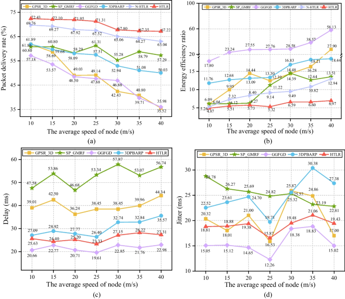
The network mobility comparison when node number = 100, the average speed of node changes from 10 m/s to 40 m/s, and simulation time = 200 s. a Packet delivery rate. b Energy efficiency ratio. c Delay. d Jitter

To further demonstrate the effectiveness of hedge transfer learning, Wilcoxon test is used to compare N-HTLR with HTLR mainly. Generally, when the average speed of node changes, these results still indicate that HTLR could ensure QoS. The explanations are as follows.
-
As a nonparametric statistical test, Wilcoxon test is widely used in various fields, which could compare two paired group datasets and computes the difference with significance level. In this paper, the significance level of Wilcoxon test is 0.05. When the p value result of Wilcoxon test is less than significance level, these two datasets are statistically significant.
-
As shown in Tables 3 and 4, the symbols of (+), (≈), and (−) indicate that HTLR is superior to, approximately equivalent to, and inferior to one compared protocol, respectively. According to 20-run PDR (or EER) data for various node-speed scenarios (the average speed of node = 10 m/s, 15 m/s, 20 m/s, 25 m/s, 30 m/s, 35 m/s, 40 m/s), we compare HTLR with the first group of compared protocols by using Wilcoxon test. HTLR is superior to the first group in all cases. On the other hand, compared with N-HTLR, HTLR is also superior to N-HTLR in all cases. These results prove that hedge transfer learning effectively improves PDR and reduces EER.
5.3 Effect of node number
Different scale searching and reconnoitering applications require different node numbers. The node-number changes lead to a series of topology changes. The node-number increase leads to more complex topology and more frequent topology changes. On the other hand, the node-number decrease results in fewer available links. Thus, it is necessary to demonstrate the node-number change effect on HTLR.
Figure 10 presents the network performances when node number = 50 ~ 150, the average speed of node = 25 m/s, and simulation time = 200 s. With the increase of node number in Fig. 10(a) and (b), the PDR and EER performances of HTLR are better than other algorithms. Additionally, with the increase of node number in Fig. 10(a) and (b), the delay and jitter results of HTLR are similar to Fig. 9(c) and (d). When deploying fewer or more nodes, the stability of 3D network topology decreases, which is a serious challenge to HTLR. However, HTLR still obtains satisfactory results, as shown in Fig. 10. This means that HTLR effectively ensures the stability of 3D network topology and QoS, no matter for node number = 50 or node number = 150.

The node number comparison when the number of nodes changes from 50 to 150, the average speed of node = 25 m/s, and simulation time = 200 s. a Packet delivery rate. b Energy efficiency ratio. c Delay. d Jitter
To further demonstrate the effectiveness of hedge transfer learning, Wilcoxon test is also used for the node-number network changes. The significance level is also 0.05. As shown in Tables 5 and 6, when compared with N-HTLR and other protocols for different node-number scenarios (node number = 50, 75, 100, 125, and 150), HTLR is superior to N-HTLR and other protocols in all cases. This also proves that hedge transfer learning is still effective when node number changes.
6 Conclusion
To ensure QoS in 3D multimedia F ANETs, HTLR mainly uses hedge transfer learning and the multi-hop link state scheme for dynamic searching and reconnoitering applications. There are two kinds of concluding remarks as follows.
-
The expansibility of hedge transfer learning. Online data in the adjacent transfer periods is similar to each other. Because the received input information of online QLS model in the last transfer period is similar to the present received input information, online QLS model is suitable for estimating the link states in most cases. According to this kind of adjacent data similarity, the hedge principle is robust to adjust Fon and Foff for online and offline QLS models. On the other hand, compared N-HTLR with HTLR, the hedge principle improves the adaptability of hedge transfer learning. Moreover, the hedge principle could support hedge transfer learning to extend its application scope. Additionally, the hedge framework of hedge transfer learning could replace artificial neural networks with other models, such as support vector machines, extreme learning machines, deep neural networks, broad learning systems, and so on.
-
The practicality of the multi-hop link state scheme. Experimental results demonstrate that the multi-hop link state scheme is feasible to evaluate the multi-hop link states even in a distributed manner. This distributed approach is interesting to estimate link states against the unstable topology of 3D multimedia FANETs.
Generally, the structure of hedge transfer learning framework is important to ensure its good adaptability to dynamic networks and expansibility to other learning methods. The multi-hop link state scheme can indeed evaluate different link paths and reflect impacts on QoS. Therefore, HTLR can effectively overcome the instability of network topology during 3D UAV video transmission and ensure QoS.
Hedge transfer learning has proven to be an effective mechanism for integrating online and offline models. However, the current hedge framework sets weights to score each model, lacking consideration for uncertainty. In the future, we will study the new hedge transfer learning framework with at least three models to explore the heterogeneous hedge principles. Meanwhile, we should also consider various factors to adjust this new hedge framework. On the other hand, there are interesting issues that should be investigated in 3D multimedia FANETs, such as detecting link failure in complex network topology and developing a mechanism to tolerate network failure, and so on.
Data availability
All data generated or analysed during this study are included in this published article.
References
Adam SM, Hassan R (2013) Delay aware reactive routing protocols for QoS in manets: a review. J Appl Res Technol 11(6):844–850. https://doi.org/10.1016/S1665-6423(13)71590-6
Adwan A, Khaled E (2015) Real-time QoS routing protocols in wireless multimedia sensor networks: study and analysis. Sensors 15(9):22209–22233. https://doi.org/10.1007/s11831-020-09418-0
Almeida EN, Coelho A, Ruela J, Campos R, Ricardo M (2021) Joint traffic-aware UAV placement and predictive routing for aerial networks. Ad Hoc Netw 118:102525. https://doi.org/10.1016/j.adhoc.2021.102525
Avin C, Mondal K, Schmid S (2022) Demand-aware network design with minimal congestion and route lengths. IEEE/ACM Trans Netw 30:1838–1848. https://doi.org/10.1109/TNET.2022.3153586
Balachandra M, Prema KV, Makkithaya K (2014) Multiconstrained and multipath QoS aware routing protocol for MANETs. Wirel Netw 20(8):2395–2408. https://doi.org/10.1007/s11276-014-0754-6
Bayat B, Crasta N, Crespi A, Pascoal AM, Ijspeert A (2017) Environmental monitoring using autonomous vehicles: a survey of recent searching techniques. Curr Opin Biotechnol 45:76–84. https://doi.org/10.1016/j.copbio.2017.01.009
Bhardwaj V, Kaur N (2021) SEEDRP: A secure energy efficient dynamic routing protocol in FANETs. Wirel Pers Commun 120:1251–1277. https://doi.org/10.1007/s11277-021-08513-0
Dong T, Qi Q, Wang J, Liu A, Liao J (2021) Generative adversarial network-based transfer reinforcement learning for routing with prior knowledge. IEEE Trans Netw Serv Manag 18(2):1673–1689. https://doi.org/10.1109/TNSM.2021.3077249
Elsayed M, Erol-Kantarci M, Yanikomeroglu H (2020) Transfer reinforcement learning for 5G new radio mmWave networks. IEEE Trans Wirel Commun 20(5):2838–2849. https://doi.org/10.48550/arXiv.2012.04840
Entezami F, Politis C (2015) Three-dimensional position-based adaptive real-time routing protocol for wireless sensor networks. EURASIP J Wirel Commun Netw 7(1):1–9. https://doi.org/10.1186/s13638-015-0419-x
Filho JA, Rosário D, Rosário D, Santos A, Gerla M (2018) Satisfactory video dissemination on FANETs based on an enhanced UAV relay placement service. Ann Telecommun 73:601–612. https://doi.org/10.1007/s12243-018-0658-z
Fleury M, Kanellopoulos D, Qadri NN (2019) Video streaming over MANETs: an overview of techniques. Multimed Tools Appl 78(16):23749–23782. https://doi.org/10.1007/s11042-019-7679-0
Freund Y, Schapire RE (1997) A decision-theoretic generalization of on-line learning and an application to boosting. J Comput Syst Sci 55(1):119–139. https://doi.org/10.1006/jcss.1997.1504
Fu J, Cui B, Wang N, Liu X (2019) A Distributed Position-Based Routing Algorithm in 3-D Wireless Industrial Internet of Things. IEEE Trans Ind Informatics 15:5664–5673. https://doi.org/10.1109/TII.2019.2908439
Grondman I, Busoniu L, Lopes GAD, Babuska R (2012) A survey of actor-critic reinforcement learning: standard and natural policy gradients. IEEE Trans Syst Man Cybern Part C-Appl Rev 42(6):1291–1307. https://doi.org/10.1109/TSMCC.2012.2218595
Gupta L, Jain R, Vaszkun G (2016) Survey of important issues in UAV communication networks. IEEE Commun Surv Tutorials 18(2):1123–1152. https://doi.org/10.1109/COMST.2015.2495297
Hamid Z, Hussain FB (2014) QoS in wireless multimedia sensor networks: a layered and cross-layered approach. Wirel Pers Commun 75(1):729–757. https://doi.org/10.1007/s11277-013-1389-0
He C, Xie Z, Tian C (2019) A QoE-oriented uplink allocation for multi-UAV video streaming. Sensors 19(15):3394. https://doi.org/10.3390/s19153394
Heinzelman WB, Chandrakasan AP, Balakrishnan H (2002) An application-specific protocol architecture for wireless microsensor networks. IEEE Trans Wirel Commun 1(4):660–670. https://doi.org/10.1109/TWC.2002.804190
Hua J, Zeng L, Li G, Ju Z (2021) Learning for a robot: deep reinforcement learning, imitation learning, transfer learning. Sensors 21(4):1278. https://doi.org/10.3390/s21041278
Hussen HR, Choi SC, Park JH, Kim J (2019) Predictive geographic multicast routing protocol in flying ad hoc networks. Int J Distrib Sens Networks 15. https://doi.org/10.1177/1550147719843879
Iskanderani AI, Mehedi IM, Aljohani AJ, Shorfuzzaman M, Akther F, Palaniswamy T, Latif SA, Latif A, Alam A (2021) Artificial intelligence and medical internet of things framework for diagnosis of coronavirus suspected cases. J Healthc Eng 2021:3277988. https://doi.org/10.1155/2021/3277988
Jiang J, Han G (2018) Routing protocols for unmanned aerial vehicles. IEEE Commun Mag 56(1):58–63. https://doi.org/10.1109/MCOM.2017.1700326
Jiang J, Han G, Guo H, Shu L, Rodrigues JJPC (2016) Geographic multipath routing based on geospatial division in duty-cycled underwater wireless sensor networks. J Netw Comput Appl 59:4–13. https://doi.org/10.1016/j.jnca.2015.01.005
Jiang B, Yan J, Xu H, Song H, Zheng G (2019) Multimedia data throughput maximization in internet-of-things system based on optimization of cache-enabled UAV. IEEE Internet Things J 6(2):3525–3532. https://doi.org/10.1109/JIOT.2018.2886964
Khan A, Rinner B, Cavallaro A (2018) Cooperative robots to observe moving targets: review. IEEE Trans Cybern 48(1):187–198. https://doi.org/10.1109/TCYB.2016.2628161
Konda VR, Tsitsiklis JN (2003) On actor-critic algorithms. SIAM J Control Optim 42(4):1143–1166. https://doi.org/10.1137/S0363012901385691
Kumar AR, Sivagami A (2020) Fuzzy based malicious node detection and security-aware multipath routing for wireless multimedia sensor network. Multimed Tools Appl 79:14031–14051. https://doi.org/10.1007/s11042-020-08631-0
Kumari P, Sahana SK (2022) Swarm based hybrid ACO-PSO meta-heuristic (HAPM) for QoS multicast routing optimization in MANETs. Wirel Pers Commun 123:1145–1167. https://doi.org/10.1007/s11277-021-09174-9
Li R, Zhao Z, Chen X, Palicot J, Zhang H (2014) TACT: a transfer actor-critic learning framework for energy saving in cellular radio access networks. IEEE Trans Wirel Commun 13(4):2000–2011. https://doi.org/10.1109/TWC.2014.022014.130840
Li B, Yang Z, Chen D, Liang S, Ma H (2021) Maneuvering target tracking of UAV based on MN-DDPG and transfer learning. Def Technol 17(2):457–466. https://doi.org/10.1016/j.dt.2020.11.014
Lu C, Lin X (2021) Towards direct edge-to-edge transfer learning for IoT-enabled edge cameras. IEEE Internet Things J 8(6):4931–4943. https://doi.org/10.1109/JIOT.2020.3034153
Masoudifar M (2009) A review and performance comparison of QoS multicast routing protocols for MANETs. Ad Hoc Netw 7(6):1150–1155. https://doi.org/10.1016/j.adhoc.2008.10.004
Nagalingayya M, Mathpati BS (2022) Energy-efficient cooperative routing scheme with recurrent neural network based decision making system for wireless multimedia sensor networks. Multimed Tools Appl 81:39785–39801. https://doi.org/10.1007/s11042-022-12938-5
Nawaz H, Ali HM, Laghari AA (2021) UAV communication networks issues: a review. Arch Comput Method Eng 28:1349–1369. https://doi.org/10.1007/s11831-020-09418-0
Niu H, Zhao X, Li J (2021) 3D location and resource allocation optimization for UAV-enabled emergency networks under statistical QoS constraint. IEEE Access 9:41566–41576. https://doi.org/10.1109/ACCESS.2021.3065055
Ostovari P, Wu J, Khreishah A, Shroff NB (2016) Scalable video streaming with helper nodes using random linear network coding. IEEE/ACM Trans Netw 24(3):1574–1587. https://doi.org/10.1109/TNET.2015.2427161
Palacios Jara E, Mohamad Mezher A, Aguilar Igartua M, Redondo RPD, Fernández-Vilas A (2021) QSMVM: QoS-aware and social-aware multimetric routing protocol for video-streaming services over MANETS. Sensors 21:901. https://doi.org/10.3390/s21030901
Pimentel L, Rosario D, Seruffo M, Zhao Z, Braun T (2015) Adaptive beaconless opportunistic routing for multimedia distribution. International Conference on Wired/Wireless Internet Communication, pp 122–135. https://doi.org/10.1007/978-3-319-22572-2_9
Riedmiller M, Braun H (1993) A direct adaptive method for faster backpropagation learning: the RPROP algorithm. Proc IEEE Int Conf Neural Networks, pp 586–591. https://doi.org/10.1109/icnn.1993.298623
Rosario D, Zhao Z, Santos A, Braun T, Cerqueira E (2014) A beaconless opportunistic routing based on a cross-layer approach for efficient video dissemination in mobile multimedia IoT applications. Comput Commun 45:21–31. https://doi.org/10.1016/j.comcom.2014.04.002
Souza J, Jailton J, Carvalho T, Araújo J, Francês R (2019) A proposal for routing protocol for FANET: a fuzzy system approach with QoE/QoS guarantee. Wirel Commun Mob Comput 2019:1–10. https://doi.org/10.1155/2019/8709249
Srinivasulu M, Shivamurthy G, Venkataramana B (2023) Quality of service aware energy efficient multipath routing protocol for internet of things using hybrid optimization algorithm. Multimed Tools Appl. https://doi.org/10.1007/s11042-022-14285-x
Wan Z, Yang R, Huang M, Zeng N, Liu X (2021) A review on transfer learning in EEG signal analysis. Neurocomputing 421:1–14. https://doi.org/10.1016/j.neucom.2020.09.017
Wang Y, Nazir S, Shafiq M (2021) An overview on analyzing deep learning and transfer learning approaches for health monitoring. Comput Math Method Med 2021:5552743. https://doi.org/10.1155/2021/5552743
Wang M, Lin Y, Tian Q, Si G (2021) Transfer learning promotes 6G wireless communications: recent advances and future challenges. IEEE Trans Reliab 70(2):790–807. https://doi.org/10.1109/TR.2021.3062045
Wu DP, Deng LL, Wang HG, Liu KY, Wang RY (2019) Similarity aware safety multimedia data transmission mechanism for internet of vehicles. Futur Gener Comput Syst 99:609–623. https://doi.org/10.1016/j.future.2018.12.032
Xu Z, Yang D, Tang J, Tang Y, Xue G (2021) An actor-critic-based transfer learning framework for experience-driven networking. IEEE/ACM Trans Netw 29(1):360–371. https://doi.org/10.1109/TNET.2020.3037231
Zhang S, Cheng W (2019) Statistical QoS provisioning for UAV-enabled emergency communication networks. Proc IEEE GLOBECOM, pp 1–6. https://doi.org/10.1109/gcwkshps45667.2019.9024517
Zhang S, Liu J (2018) Analysis and optimization of multiple unmanned aerial vehicle-assisted communications in post-disaster areas. IEEE Trans Veh Technol 67(12):12049–12060. https://doi.org/10.1109/TVT.2018.2871614
Zhang T, Zhao S, Cheng B (2020) Multipath routing and MPTCP-based data delivery over MANETs. IEEE Access 8:32652–32673. https://doi.org/10.1109/ACCESS.2020.2974191
Zhang M, Dong C, Feng S, Guan X, Chen H, Wu Q (2022) Adaptive 3D routing protocol for flying ad hoc networks based on prediction-driven Q-learning. China Commun 19(5):302–317. https://doi.org/10.23919/JCC.2022.05.005
Acknowledgements
This work was supported by National Natural Science Foundation of China (Grant No. 61876199), National Key Research and Development Program of China (Grant No. 2022YFF0604900) and Research Initiative of Ideological and Political Theory Teachers (No. 20SZK10013001).
Author information
Authors and Affiliations
Corresponding author
Ethics declarations
Confect of interest
The authors confirm that this work is original and has either not been published elsewhere, or is currently under consideration for publication elsewhere. None of the authors have any competing interests regarding the publication of this article.
Additional information
Publisher’s note
Springer Nature remains neutral with regard to jurisdictional claims in published maps and institutional affiliations.
Rights and permissions
Springer Nature or its licensor (e.g. a society or other partner) holds exclusive rights to this article under a publishing agreement with the author(s) or other rightsholder(s); author self-archiving of the accepted manuscript version of this article is solely governed by the terms of such publishing agreement and applicable law.
About this article

Cite this article
Zhang, H., Lv, X., Liu, Y. et al. Hedge transfer learning routing for dynamic searching and reconnoitering applications in 3D multimedia FANETs. Multimed Tools Appl 83, 7505–7539 (2024). https://doi.org/10.1007/s11042-023-15932-7
Received:
Revised:
Accepted:
Published:
Issue Date:
DOI: https://doi.org/10.1007/s11042-023-15932-7