Subdivide and Conquer: Adapting Non-Manifold Subdivision Surfaces to Surface-Based Representation and Reconstruction of Complex Geological Structures

Abstract

Methods from the field of computer graphics are the foundation for the representation of geological structures in the form of geological models. However, as many of these methods have been developed for other types of applications, some of the requirements for the representation of geological features may not be considered, and the capacities and limitations of different algorithms are not always evident. In this work, we therefore review surface-based geological modelling methods from both a geological and computer graphics perspective. Specifically, we investigate the use of NURBS (non-uniform rational B-splines) and subdivision surfaces, as two main parametric surface-based modelling methods, and compare the strengths and weaknesses of the two approaches. Although NURBS surfaces have been used in geological modelling, subdivision surfaces as a standard method in the animation and gaming industries have so far received little attention—even if subdivision surfaces support arbitrary topologies and watertight boundary representation, two aspects that make them an appealing choice for complex geological modelling. It is worth mentioning that watertight models are an important basis for subsequent process simulations. Many complex geological structures require a combination of smooth and sharp edges. Investigating subdivision schemes with semi-sharp creases is therefore an important part of this paper, as semi-sharp creases characterise the resistance of a mesh structure to the subdivision procedure. Moreover, non-manifold topologies, as a challenging concept in complex geological and reservoir modelling, are explored, and the subdivision surface method, which is compatible with non-manifold topology, is described. Finally, solving inverse problems by fitting the smooth surfaces to complex geological structures is investigated with a case study. The fitted surfaces are watertight, controllable with control points, and topologically similar to the main geological structure. Also, the fitted model can reduce the cost of modelling and simulation by using a reduced number of vertices in comparison with the complex geological structure.

Graphical Abstract

1 Introduction

Surface representation is one of the common concepts between geology and computer graphics. According to Botsch et al. (2010), implicit and parametric representations can be considered as the two main types of surface representations, where in both types, the surface is defined by a specific function: implicit surfaces are defined by a scalar-valued function, and the aim is to find a zero level set, whereas a parametric surface is defined by a vector-valued function, and the aim is to convert the three-dimensional to two-dimensional models in the parametric domain. A parametric representation has advantages over an implicit representation in the direct representation of surfaces and it can present details in a more compact and modifiable form but at the cost of requiring more effort for calculating spatial queries (Botsch et al. 2010). Similar to applications in computer graphics, parametric surface-based geological and reservoir representations are defined by the surrounding surfaces (Caumon et al. 2009; Deveugle et al. 2011; Graham et al. 2015a, b; Jackson et al. 2014, 2015; Jacquemyn et al. 2019; De Kemp 1999; Wellmann and Caumon 2018). In contrast to grid-based implicit geomodelling, one of the key advantages of parametric surface-based methods is that most of the critical details of the model, such as heterogeneity, will be well maintained since there is no need to consider the “averaged value” within the cells (Jacquemyn et al. 2019; Pyrcz et al. 2009; Ruiu et al. 2016; Zhang et al. 2009). In addition to implicit and parametric surface-based models, previous studies have investigated hybrid methods (Hassanpour et al. 2013; Pyrcz et al. 2009; Ruiu et al. 2016). Although hybrid approaches lead to more acceptable and faithful results, the need for a high-resolution grid is a limitation of these methods (Jacquemyn et al. 2019).

From a computer graphics point of view, spline surfaces and subdivision surfaces are two types of parametric surface-based representations (Botsch et al. 2010). Spline surfaces are the usual standard for computer-aided design (CAD), while subdivision surfaces are primarily used in computer gaming, animation and the film industry (Botsch et al. 2010; Cashman 2010). Generally, subdivision surfaces and non-uniform rational B-splines (NURBS) both yield controllable freeform representations, but in different ways; NURBS emphasise the smooth manipulation of the model, whereas subdivision surfaces tend to release the model from topological limitations (constraints) (Cashman 2010) and enable surfaces with arbitrary topology (Botsch et al. 2010). The term topology refers to the connection between different elements of the model, and in geological modelling, it is a vital constraint for most geological procedures and actions, including fluid flow, heat transfer and deformation (Burns 1975; Deutsch 1997; Jones 1989; Mallet 1997; Thiele et al. 2016).

Previous studies using NURBS for geological, reservoir and fracture modelling showed that NURBS had been used for various goals in this context (Börner et al. 2015; Caumon 2010; Corbett et al. 2012; Fisher and Wales 1992; Florez et al. 2014; Geiger and Matthäi 2014; Gjøystdal et al. 1985; Jackson et al. 2015; Jacquemyn et al. 2019; de Kemp and Sprague 2003; De Kemp 1999; Paluszny et al. 2007; Sprague and De Kemp 2005; Zehner et al. 2015). However, subdivision surfaces have rarely been used in geological and reservoir modelling. Chen and Liu (2012) investigated geological modelling using the subdivision surface method. Although their work deserves appreciation, the authors did not explain the practical details of this approach and offered no explanation for the distinction between using spline surfaces and subdivision surfaces in parametric surface-based geological modelling.

NURBS support non-uniform parameterisation by using the knot vector, which can change the degree of the curve or surface at any knot (Ruiu et al. 2016; Cashman 2010). Although the classical subdivision scheme cannot support non-uniform parameterization, this scheme provides a significant benefit over NURBS by supporting watertight modelling with arbitrary topology, since it eliminates the procedure of stitching and editing different surface patches (Cashman 2010). Watertight modelling is a type of modelling in which the surfaces of the model have sealed interactions with all surrounding surfaces, resulting in the generation of closed volumes.

There are solutions (methods) that exploit the advantages of both NURBS and subdivision schemes, such as NURBS compatible with subdivision surfaces (Cashman 2010), non-uniform recursive subdivision surfaces (Sederberg et al. 1998) and T-NURCCs (non-uniform rational Catmull-Clark surfaces with T-junctions) (Sederberg et al. 2003).

In reservoir modelling, NURBS “curves” have been used to represent well trajectories (Jacquemyn et al. 2019). Additionally, NURBS “surfaces” have been used for modelling sinuous channels by tensor products between two NURBS curves: one NURBS curve for defining the cross-section and one curve for the trajectory of the channel (Ruiu et al. 2016). Therefore, non-uniform parameterisation can make NURBS suitable for modelling structures with several different meanders (curvatures) along a path (trajectory). On the other hand, subdivision surfaces have fewer difficulties in modelling watertight surface intersections, which is more beneficial for channels intersecting with each other or layers. Therefore, one possibility of taking advantage of both NURBS and subdivision surfaces in geological modelling is to use both of these methods simultaneously, for example, for generating the meanders.

A surface is called a manifold surface if each of the points of the surface has a neighbourhood homeomorphic to an open disc (Theoharis et al. 2008). Therefore, “non-manifold surfaces” are complex surfaces when the vicinity of each point is not homeomorphic to an open disc. In a triangle mesh, an edge is called a “non-manifold” if it is incident to more than two triangles. The non-manifold structures need more complex algorithms for the representations (Rossignac and Cardoze 1999). Figure 1 shows one of the common examples of non-manifold surfaces in geological modelling, which contains three surfaces shared by one edge. The green edge and yellow vertices are non-manifold edges and vertices, respectively. From the geological modelling point of view, contacts between geological interfaces where multiple faces of the mesh are shared by one edge (e.g., intersection between faults or between faults and horizons) are common examples of non-manifold surfaces (Caumon et al. 2004). Also, complex geological structures commonly comprise multiple intersecting surfaces (Dassi et al. 2014). Therefore, non-manifold topology is crucial for the representation of complex geological and reservoir modelling. In this paper, the term “non-manifold” refers to non-manifold surfaces.

Classical subdivision surface algorithms cannot support non-manifold topologies. However, the support for arbitrary topologies and the other excellent features of subdivision surfaces make it worthwhile to use modified subdivision surfaces for non-manifold geological topologies. This work aims to contribute to complex geological and reservoir modelling using a non-manifold subdivision surface algorithm (surface-based geological modelling). Figure 2 represents the control mesh and the smooth surfaces of a common non-manifold geological structure by applying the non-manifold subdivision surface algorithm.

Fig. 1

Representation of the procedure to generate a geological structure with non-manifold topology by using a surface-based non-manifold subdivision surface method from a coarse mesh: a Control mesh with the control points (purple) and the edges with different crease sharpness values (blue and red). b Smooth and subdivided mesh generated by repeatedly applying a subdivision surface algorithm modified by control points (purple). c Rendered version of the final mesh

Fig. 2

Three faces share one edge, a typical example of a non-manifold shape. Non-manifold vertices (yellow) and edge (green) with manifold vertices (purple) and edges (blue)

NURBS and subdivision surfaces are also used to fit smooth surfaces with mesh or dense data (Panozzo et al. 2011; Ma et al. 2004). NURBS are primarily utilised for topologically simple cases since managing the connections between different patches of NURBS in topologically complex cases is difficult. However, the subdivision surfaces scheme generates structures with arbitrary topology and equal precision as NURBS (Ma et al. 2015). In this paper, solving the reverse problem by fitting smooth surfaces to complex geological and reservoir structures is investigated. Generated models by the non-manifold subdivision surface method are topologically similar to the initial geological structures and exploit all advantages of surface-based modelling (e.g., grid-free, smooth and controllable with some control points). Also, they have fewer vertices which can reduce the cost of processing in complex geological simulations.

2 Methods

2.1 Spline Surfaces

Spline surfaces are a standard method for representing high-quality freeform surfaces, which are generated by mapping from a rectangular, parametric domain (u,v) to the ${R}^{3}$ (x, y, z) domain. A general spline surface of bi-degree $n$ can be obtained by Eq. (1) (Botsch et al. 2010).

$$(u,v)\to \sum_{i=0}^{m}\sum_{j=0}^{k}{c}_{ij}{ N}_{i}^{n}\left(u\right){N}_{j}^{n}\left(v\right),$$

(1)

where ${c}_{ij}$ are the control points in ${R}^{3}$, and $m+1$ and $k+1$ are the numbers of control points in the $u$ and $v$ directions, respectively. Additionally, ${N}_{i}^{n}(u)$ and ${N}_{i}^{n}(v)$ are spline blending functions in the $u$ and $v$ directions, such as B-spline (basis spline) functions. NURBS (non-uniform rational B-spline) surfaces are famous spline surfaces that are useful for making high-quality, freeform and editable surfaces (Fig. 3) (Botsch et al. 2010).

Fig. 3

Representation of the different NURBS surfaces: control mesh (blue) and NURBS surface (purple). Single NURBS surfaces are limited to topologically similar surfaces to a sheet, b cylinder or c torus surfaces (DeRose et al. 1998)

Theoretically, NURBS surfaces are parametric surfaces that can be made according to the numbers of weighted points (control points), parametric knot vectors and specific interpolation degrees between the control points (Piegl and Tiller 1996).

NURBS surfaces have three critical features, as follows:

• (1) B-spline surface: B-spline or basis spline surfaces are piecewise parametric surfaces (see Appendix 2.2) based on basis spline functions. They include control points and the surface affected by the control points.

• (2) Rational: This means that the control points of the B-spline have weight values that can change the effect of a control point on a surface.

• (3) Non-uniform: This feature makes NURBS suitable for several practical goals (Cashman 2010). NURBS surfaces are combinations of polynomial sections joined at specific positions, which are knots (Piegl and Tiller 1996). The knots make a surface locally modifiable while the surface remains smooth (except when the knot multiplicity increases), which means that changing the position or the weight of any specific control point can affect only the related part of the mesh (not the entire mesh) (Piegl and Tiller 1996). If the knots are equally positioned, this is equivalent to a uniform B-spline. Otherwise (if the knots are arbitrarily distributed), it is a non-uniform B-spline (NURBS) surface.

2.2 Limitations of NURBS Surfaces

• I. The main restriction of any single surface that is made by planar parameterisation (a rectangular grid), such as NURBS, is the limitation on the construction of surfaces that are topologically similar to a sheet, cylinder or torus (Fig. 3) (Cashman 2010; DeRose et al. 1998). Therefore, to create a model with a complex topology, many NURBS patches have to be smoothly connected (by stitching NURBS patches together). Multiple connections between surface patches in addition to topological or geometric constraints make the modelling procedure more complex (Botsch et al. 2010; Cashman 2010). As a result of the strict rectangular topology of NURBS surfaces, trimming the NURBS patches before stitching is fundamental during complex shape modelling, which can create unavoidable gaps between trimmed NURBS patches (Shen et al. 2014; Sederberg et al. 2008).

• II. Modifying classical NURBS surfaces, such as adding more control points, will influence an entire row or column of control points (Botsch et al. 2010). Indeed, preserving the grid structure of NURBS surfaces during local refinement is challenging (DeRose et al. 1998). It should be mentioned that T-splines, as a generalisation of the NURBS, offer local refinement and can markedly decrease the number of control points (Sederberg et al. 2004).

2.3 Subdivision Scheme

The subdivision scheme was created to overcome the difficulties of constructing smooth surfaces by supporting arbitrary topology (Zorin and Schröder 2001; Catmull and Clark 1978; Doo and Sabin 1978). The primary idea behind the subdivision scheme is to use the initial mesh to simulate a smooth structure by refinements. In practice, the modifications are carried out repeatedly until the simulated curve/surface is fine enough. The vertices of the initial mesh (control mesh) control the shape of the final smooth structure.

Figure 4a represents a simple control mesh, a cube with eight vertices, 12 edges and six faces. Applying the subdivision surface algorithm over the control mesh leads to the generation of the smooth mesh from the control mesh (Fig. 4b). Increasing the subdivision iteration leads to an increase in the smoothness and the number of vertices of the generated mesh (Fig. 4c). Moreover, by changing the position of the control points, the generated mesh changes smoothly (Fig. 4d).

Fig. 4

An example of a simple subdivision surface method, generating a smooth mesh (green edges) by regularly applying the subdivision scheme. a The original mesh (control mesh) has eight purple vertices (control points) and 12 red edges. b and c Applying the subdivision surface algorithm to the original mesh one and three times. d Deformation of the resulting mesh by adapting the position of the control points

The subdivision surfaces scheme not only overcomes the limitations of NURBS by defining smooth and controllable surfaces that need no trimming for arbitrary topologies, but is also computationally efficient and suitable for complex geometry (Zorin 2000).

2.4 Subdivision Algorithm: the Combination of Splitting and Averaging

For generating smooth curves/surfaces in each refinement, the subdivision scheme follows two steps based on mathematical rules; splitting and averaging. In the splitting step, new vertices are inserted on the curve/surface, and in the averaging step, the positions of the vertices are updated. This section comprehensively explains these two steps for generating smooth curves and surfaces, respectively.

2.4.1 Subdivision Curves

The aim is to continuously refine the polygon (control mesh) to generate a smooth curve with an arbitrary degree. The vertices of the control mesh are the control points of the final smooth curve. Figure 5 shows an example of the generation of a cubic B-spline subdivision curve generated by a subdivision algorithm. The control mesh has four vertices (orange vertices) (Fig. 5a), and the smooth curve (purple curve) is generated after applying a subdivision refinement twice (Fig. 5b). The final curve is the combination of four curves of degree three (cubic B-splines) stitched together (Fig. 5c). By increasing the number of refinements, the final curve will be smoother, but the degree of the curve will not change. The step-by-step workflow for the generation of the subdivided curve is explained in the next step (Fig. 5).

Fig. 5

Generation of a cubic B-spline subdivision curve. a The control mesh with four control points (orange vertices). b The smooth curve after subdivision twice. c The smooth curve is the combination of four curves (yellow, green, blue and red) of degree three

Step-by-Step Workflow for Generation of the Subdivided Curve

• (1) Splitting step

  New vertices are inserted in the middle of each edge, and then the vertices are connected (Fig. 6).

• (2) Averaging step

  The location of each vertex is updated by applying the averaging mask (i.e., the new location is the weighted average of the current location of the vertex and the location of the neighbours). The averaging mask is based on the Lane-Riesenfeld algorithm, which computes the averaging mask of each point of the polygon for generating B-splines of degree ${\varvec{n}}+1$ using Eq. (2) (Vouga and Goldman 2007; Lane and Riesenfeld 1980).

$$w= \frac{1}{{2}^{n}}\left\{ \left(\begin{array}{c}n\\ 0\end{array}\right), \left(\begin{array}{c}n\\ 1\end{array}\right), \left(\begin{array}{c}n\\ 2\end{array}\right),\dots ,\left(\begin{array}{c}n\\ n\end{array}\right) \right\},$$

(2)

where $\left(\begin{array}{c}n\\ k\end{array}\right)$ is the binomial coefficient of the $n$ and $k$.

Fig. 6

Splitting step for the generation of a cubic B-spline subdivision curve. a The control mesh with four control points (orange vertices). b Inserting new vertices (purple vertices) on the middle of each edge. c Connecting all vertices to each other

For example, Fig. 7 shows the averaging step for generating the cubic B-spline curve. The cubic B-spline subdivision mask indicates the degree $=3$; therefore, $n=2$. By importing $n=2$ into Eq. (2), the averaging mask for each vertex and two adjacent vertices is $=$ $\frac{1}{4}\left\{1, 2, 1\right\}$. Therefore, the new position for each vertex (${p}_{new}$) can be calculated by

$${p}_{new}=\frac{1}{4}\left(1*{d}_{1}+2*p+1*{d}_{2}\right),$$

(3)

where ($p$) is the location of the existing vertex, and $({d}_{1},{d}_{2})$ are the locations of two neighbour vertices (Fig. 7c). By applying the averaging mask to all vertices of Fig. 7a, the positions of all of the vertices are updated. Finally, by repeatedly splitting and averaging steps (subdivision refinement), a series of smoother curves (cubic B-spline curves) will be generated (Fig. 8).

Fig. 7

Averaging step for cubic B-spline subdivision. a Control mesh associated with midpoint vertices (purple vertices). b Generating the smooth curve (purple curve) by updating the position of all the vertices based on averaging step. c Representation of averaging step by cubic B-spline subdivision mask

Fig. 8

Generation of cubic B-spline curves after applying one and two times subdivision curves algorithm. a Control mesh with four control points (orange vertices); b Generating the smooth curve (purple curve) after applying one-time subdivision curve algorithm; c Generated the smooth curve (purple curve) after applying two times subdivision curve algorithm

2.4.2 Subdivision Surfaces

Extending the subdivision curve approach to surfaces leads to the subdivision surface approach. Subdivision surfaces repeatedly refine the coarse mesh (control mesh) to generate a smooth surface. Similar to the subdivision curve, subdivision surfaces follow splitting and averaging steps at each refinement stage. The vertices of the control mesh are the control points of the final smooth surface. There are different subdivision surface schemes, such as the Catmull-Clark scheme (Catmull and Clark 1978) for quadrilateral meshes and the Loop scheme (Loop 1987) for triangular meshes. In this section, the Loop algorithm is explained. For completion, the Catmull-Clark scheme is described in Appendix 1.

2.4.2.1 Loop Subdivision Scheme

The Loop scheme, defined by Loop (1987), builds smooth surfaces based on triangle meshes by using splitting and averaging steps in each refinement stage.

Step-by-step workflow for the generation of the subdivided surfaces:

• (1) Splitting step

  Each triangle of the control mesh is split into four triangles by inserting a new vertex on the midpoint of each edge (Fig. 9).

• (2) Averaging step

  The averaging step in the Loop algorithm consists of two parts:

  • (Ι) Updating the position of the new midpoint vertices generated from the splitting step (purple vertices)

  Figure 10 shows the new midpoint ($e$) of an edge surrounded by four existing vertices (${d}_{1},{d}_{2},{d}_{3},{d}_{4}$). The Loop algorithm applies Eq. (4) (weighted averaging of the ${d}_{1},{d}_{2},{d}_{3},{d}_{4}$) to determine the new location of the vertex $e$ (Loop 1987).

  Fig. 9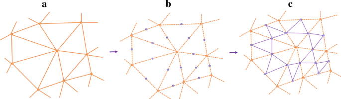

  

  Splitting step for generation of subdivision surfaces by Loop subdivision scheme. a The control mesh with control points (orange vertices). b Inserting new vertices (purple vertices) on the midpoint of each edge. c Connecting vertices to each other

  Fig. 10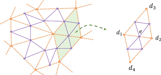

  

  Averaging step of generating the smooth surface by Loop subdivision scheme

  $$e=\frac{3}{8}\left({d}_{1}+{d}_{2}\right)+\frac{1}{8}\left({d}_{3}+{d}_{4}\right).$$

  (4)

(II) Updating the position of the existing vertices (orange vertices)

Figure 11a shows an existing vertex ($v$) with k adjunct vertices (${p}_{1},{p}_{2}$,${p}_{3},\dots ,{p}_{k}$). For updating the position of the vertex ($v$), the Loop algorithm proposes the use of a weighted average of the vertex $v$ and ${p}_{1},{p}_{2}$,${p}_{3},\dots ,{p}_{k}$ (Loop 1987).

$${v}_{new}=v*\left(1-k\beta \right)+\beta \sum_{1}^{k}{p}_{k},$$

(5)

where

Fig. 11

Averaging step of generating the smooth surface in the Loop subdivision scheme. a Representation of an existing vertex ($v$) with $k$ adjunct vertices. b Example of an existing vertex ($v$) around which there are seven adjunct vertices

$$ \beta = \frac{1}{k}\left( {\frac{5}{8} - \left( {\frac{3}{8} + \frac{1}{4}cos\frac{{2\pi }}{k}} \right)^{2} } \right). $$

(6)

To put it more simply, the Loop algorithm assigns the weight $\left(1-k\beta \right)$ to the location of the existing vertex and weight $\beta$ to the location of each adjacent vertex in the averaging step. For example, Fig. 11b shows the vertex $v$ which has seven adjunct vertices, and therefore, $k=7$. Based on Eq. (6), $\upbeta =$ 0.049, which means that each of the adjacent existence vertices around $v$ has a weight = 0.049 and $v$ has a weight = 0.65 during the averaging step.

As an alternative, Warren (1995) proposed an additional weighting scheme for the calculation of $\upbeta$ when the number of adjacent vertices (k) is greater than 3 by

$$\upbeta =\frac{3}{8k}.$$

(7)

By repeating the splitting and averaging steps, the final surface will be smoother, and the number of vertices will increase.

2.5 Piecewise Smooth Subdivision Surfaces

Representation of objects consisting of sharp features by smooth subdivision algorithms leads to unsatisfactory results. Hoppe et al. (1994) proposed adding new rules for the representation of the creases and corners to the Loop subdivision scheme (which can be implemented for the Catmull-Clark scheme) in which the new location of the vertex $v$ depends on the number of connected sharp edges as represented in Table 1 (DeRose et al. 1998).

Table 1 The rules for updating the positions of vertices connected to sharp edges (DeRose et al. 1998). Please see Hoppe et al. (1994) for more information

The piecewise subdivision surface method presents the acceptable rules for generating the sharp regions of the model. However, in complex geological modelling, it is vital to model the semi-sharp regions which are not quite sharp. In Sect. 2.6, we comprehensively explain the solution for this problem by using the semi-sharp subdivision surfaces method.

2.6 Subdivision Surfaces with Semi-Sharp Creases, A Tool for Modelling Complex Geometries

Modifying the classical subdivision algorithm allows smooth surfaces to have sharp features such as creases and corners (DeRose et al. 1998; Hoppe et al. 1994). Although real-world models such as geological structures do not have entirely sharp features, managing and controlling the sharpness of creases and corners during the subdivision procedure can be very useful in building complex structures. A crease can be created on the mesh by changing the mesh shape (e.g., by applying subdivision approaches or pulling the mesh) while pinching the specific vertices or edges of the mesh (Fig. 12). With more freedom given to the related vertices or edges, the sharpness of the crease decreases.

Fig. 12

Creating creases on a mesh by applying the subdivision surfaces algorithm three times. a Control mesh. b All edges of the cube are smooth edges (red edges). c Four edges are crease edges (blue edges), and eight edges are smooth (red edges)

Practically, during the subdivision of surfaces, it is possible to consider the average crease sharpness value for each edge of the mesh. These numbers can show the resistance of the vertices of the edges to mesh modification algorithms, such as resistance to smoothing by subdivision surfaces (if more than one edge is connected to the vertex, the average value should be considered). The higher the crease sharpness value, the sharper the crease. This value can be between zero and infinity, where zero indicates a smooth crease (DeRose et al. 1998). Adjusting the crease sharpness allows for greater flexibility in modelling different geometric objects.

As disused in Sect. 2.5, Hoppe et al. (1994) defined the new rules for the generation of sharp regions during the subdivision procedure. However, complex structures may consist of semi-sharp regions which are not fully sharp. DeRose et al. (1998) generalised the method proposed by Hoppe et al. (1994) for updating the position of the vertices based on semi-sharp subdivision surfaces, which is explained in Table 2. For more information, please see DeRose et al. (1998).

Table 2 The rules of the semi-sharp creases scheme for updating the positions of vertices (DeRose et al. 1998)

2.7 Subdivision Surfaces Compatible with Non-Manifold Topologies

Classical subdivision surfaces cannot support non-manifold shapes, since these shapes contain at least one local geodesic neighbourhood, which makes the topology challenging and incompatible with many methods, including subdivision surfaces (Botsch et al. 2010). In fact, some vertices and edges will not follow the classical subdivision algorithms (irregular vertices and edges). Therefore, an adapted “non-manifold subdivision algorithm” has been proposed to combine the advantages of the subdivision surface method such as the application to arbitrary topology and still produce watertight volumes for non-manifold shapes. The non-manifold subdivision surfaces algorithm defined by Ying and Zorin (2001) includes several detailed rules and covers a wide range of non-manifold problems in computer graphics. In this section, the practical rules related to modelling the intersections between several surfaces, with a particular interest in typical geological modelling geometries, are explained (Figs. 1 and 13). For additional cases, see Appendix 2 and Ying and Zorin (2001).

Fig. 13

Representation of simple and complex non-manifold vertices

Figure 13 shows an example of the intersection of the surfaces. These surfaces can be different faults or intersections between a geological horizon and a fault. In this example, the edges and vertices on the shared boundary of the surfaces are non-manifold. If two non-manifold edges (blue edges) meet each other at one vertex, that vertex will be a simple non-manifold vertex (pink vertex); otherwise, it is a complex non-manifold vertex (yellow vertices).

Ying and Zorin (2001) mention that in the averaging step of subdivision surfaces for regular (manifold) vertices, the standard Loop algorithm should be applied. They also note that if the vertex is a simple non-manifold, the cubic B-spline subdivision algorithm (as mentioned in Sect. 2.4) should be used, and if the vertex is a complex non-manifold, in most cases, a vertex will be fixed (the position of the vertex during the subdivision procedure will not be changed). Additionally, if the edge is singular (non-manifold edges, blue edges), it should be subdivided at the midpoint; otherwise, it should follow the standard Loop algorithm. For more information, see Ying and Zorin (2001). These considerations enable the representation of a wide range of non-manifold geological geometries.

3 Parametric Surface-Based Geological Modelling

Gjøystdal et al. (1985), Caumon et al. (2004) and Jacquemyn et al. (2019) defined geological domains as closed volumes, which are mostly limited by interacting surfaces. These surfaces must represent the correct topology of the geological model and should have a watertight relationship with other surfaces. To build such closed volumes with NURBS, different NURBS surfaces (patches) are needed to interact with each other in different ways (Jacquemyn et al. 2019). Also, the relationships between independent NURBS surfaces violate geological principles, and we need to consider approaches for remedying this, such as building parametric surfaces for the entire domain and modifying the model by trimming, cutting or extrapolating the surfaces (Wellmann and Caumon 2018). As mentioned previously, according to several computer graphics references (Botsch et al. 2010; Cashman 2010; DeRose et al. 1998), the need for connecting, trimming and stitching different NURBS patches to each other to build a complex model is one of the limitations of NURBS. However, the need for stitching and trimming separate surface patches to make watertight closed-volume surfaces is eliminated in the subdivision surface approach by building surfaces and volumes with arbitrary topology (Cashman 2010).

To build surface-based geological structures using subdivision surfaces, we propose the following steps:

• (1) In the first step, the control mesh is generated. The control mesh is a seamless mesh, topologically similar to the geological structure. The vertices of the control mesh are the control points of the final mesh. If the geological structure contains multiple layers or faults, the control mesh should be defined as one seamless mesh including these features.

• (2) Based on the geological structure, the sharpness of the crease of each edge (crease sharpness value) is specified and assigned.

• (3) The non-manifold subdivision algorithm is applied. This step should be repeated until a final model with desired smoothness is obtained.

• (4) If needed, the control mesh is edited by changing the positions of the control points or the crease sharpness values of the edges to reach the final goal (geological structure).

3.1 Different Types of Geological Surface Interactions

There are three different types of geological surface interactions to generate the geological domains (Jacquemyn et al. 2019).

3.1.1 Creating Closed Volumes by Joining Surfaces at Their Edges

In this case, there are at least two surfaces that should be connected exactly on their edges (boundaries) to produce a watertight volume (e.g., sinuous channels, Fig. 14). Jacquemyn et al. (2019) explained how to use NURBS to build these complex shapes (Fig. 14a). In their work, two different surfaces that have exactly the same edge geometries are connected to each other. However, as mentioned in Sect. 2.2, modelling becomes more complicated by connecting (stitching) multiple NURBS patches along with topological and geometric constraints (Botsch et al. 2010; Cashman 2010). Although Jacquemyn et al. (2019) mentioned solutions such as using the degree elevation procedure or adding more control points (which is one of the limitations of classical NURBS), and Ruiu et al. (2016) suggested increasing the multiplicity of the knots (which results in reduced continuity, see Cashman 2010), using a subdivision surface method has fewer difficulties because of its inherent features, such as supporting arbitrary topology and watertight modelling.

Fig. 14

Building watertight channels by NURBS and subdivision surfaces (our approach). a Using NURBS to join surfaces at their edges to create closed volumes (Jacquemyn et al. 2019). b Building a channel using subdivision surfaces and defined crease sharpness values with subdivision stages. The crease sharpness value for each red and blue edge is zero and 1, respectively

To build similarly closed volumes based on the subdivision surface method, first, the coarse and seamless control mesh is defined (Fig. 14b). In the second step, the crease sharpness values of all edges are specified. For example, in the sinuous channel case, because the top face of the channel is flat, the top edges on the sides of the channel are set to fully resist smoothing during the subdivision procedure, and their crease sharpness values are set to 1 (blue edges). Also, most of the other edges should be smoothly subdivided; therefore, their crease sharpness values are zero (red edges). In the third step, the subdivision algorithm based on the crease sharpness value of each edge is applied with four refinement stages. The final subdivided surface is a watertight and smooth channel, which can be controlled by the control points (Fig. 14b).

3.1.2 Distorted (Warped) Surfaces

Warped geological structures can be considered as a type of complex geological setting (in a geometric modelling sense) and are observed in nature in different ways, as described below:

• (Ι) Warped geological surfaces, generated from geological phenomena such as folding and faulting.

• Warped surfaces can pose challenges in geological modelling. Since the abilities of the selected method for modelling, such as the flexibility and consistency of structures (supporting arbitrary topologies), can play an essential role in the entire modelling process, using subdivision surfaces instead of NURBS can lead to fewer difficulties, especially in layered warped structures. Figure 15 shows a model of a faulted fold created by Catmull-Clark subdivision surfaces. Due to the suggested subdivision surfaces algorithm, the control mesh (two separate cages) is first defined (Fig. 15a). In the next step, the sharpness of the crease of each edge is assigned (the blue and red edges have crease sharpness values equal to 1 and zero, respectively). Finally, the subdivision surface algorithm is applied with four stages.(Fig. 15b)

• (ΙΙ) Warped geological surfaces associated with other surfaces that have geometric connections with them.

Fig. 15

An example of a faulted fold obtained through the use of subdivision surfaces. a During the smoothing procedure, the sharpness of the crease value of each edge affects the mesh representation (the blue and red edges have crease sharpness values equal to 1 and zero, respectively). b The final smooth model after applying the subdivision algorithm

Some geological settings require the modelling of hierarchies of geometries, for example, in deformed layer stacks or sedimentary sequences in a channel. Such structures can be considered through combinations of at least two NURBS surfaces with different grid structures that need to be matched (by warping one of the surfaces) to obtain the new structure. Jacquemyn et al. (2019) defined a procedure for building such structures based on NURBS. In their method, the positions of the control points of the surface to be warped need to be adapted to the parent surface(s). However, this adaption can be expensive due to the limitations of NURBS, such as the difficulties in adding more control points (as mentioned before, this is only possible by splitting parameter intervals that affect an entire row or column of the control mesh; see also Botsch et al. 2010) and problems in trimming. The subdivision surface approach, unlike NURBS, first considers one comprehensive topology (control mesh) consisting of a watertight structure for both surface topologies together, the warped and parent topologies (instead of two separate topologies), and then refines the model by assigning a specific crease sharpness value to each edge and applying the subdivision algorithm, leading to a watertight mesh with a consideration of the geometric hierarchies.

3.1.3 Truncated Hierarchically Organized Surfaces

An additional common geometric setting in geology is the truncation of one geological object by another object, for example, along unconformities or intrusive bodies. In these cases, hierarchically organized surfaces have to be truncated against each other to obtain watertight subvolumes (surfaces that terminate on the body of another surface, e.g., clinoform surfaces). Jacquemyn et al. (2019) provide instructions to model such topologies with NURBS (e.g., model from higher hierarchal levels to lower levels because the coordinates of lower levels are relative to higher levels; then, perform the termination operation) (Fig. 16a). However, several authors point out that using NURBS for modelling such complex structures is challenging because of the undesirable gaps arising at the boundaries between surfaces (Urick et al. 2019; Pungotra et al. 2010; Sederberg et al. 2008, 2003; Chui et al. 2000). Generally, the inherent difficulties associated with NURBS surfaces, such as limitations in stitching and problems in trimming the surfaces for building watertight volumes, complicate the entire modelling process. Here also, a modelling approach using subdivision surfaces can address this limitation. First, a simple watertight layered mesh (control mesh) is defined with a consideration of the non-manifold topologies (Fig. 16b). As before, crease sharpness values are assigned and the non-manifold subdivision surface method is applied to obtain the desired result.

Fig. 16

a Termination of hierarchically arranged surfaces by NURBS for the basal surface of a channelized body (Jacquemyn et al. 2019). b Applying non-manifold subdivision surfaces to create hierarchically arranged surfaces

4 Surface Reconstruction Using the Non-Manifold Subdivision Algorithm

In addition to generating new geometric representations with the subdivision algorithm, it is also possible to obtain reconstructions of existing models—for example, with the aim to obtain fully watertight meshes for further use in process simulations. This process requires special care, as it requires matching geometric objects through adjustments of control points and crease sharpness values. We therefore propose the following steps to achieve this aim and show the application to a geological model.

4.1 Workflow for Surface Reconstruction

The first step is generating a suitable control mesh considering the outstanding features of the input mesh (e.g., local maxima, minima, saddle, umbilics and ridge points). The control mesh needs to have a similar topology as the target geological model, while it can be coarser with fewer vertices. The specific features should be captured by considering related parameters such as principal curvatures or face normals (Ma et al. 2015; Marinov and Kobbelt 2005; Kälberer et al. 2007). Then the surface intersections are evaluated carefully and, if necessary, additional control points are generated to support the intersections and watertight modelling. In the end, the control points are connected, which leads to the generation of the control mesh.

The second step is defining smooth parts of the model (e.g., folds) by assigning unique crease sharpness values to each edge of the control mesh, and then a suitable subdivision surface algorithm is applied to the control mesh to perform smoothing. The third step is fitting the watertight smooth surfaces to the input mesh. Minimizing the sum of the squared distances between the vertices of the input mesh (geological structure) and the approximated mesh is a common approach for fitting a mesh (Mallet 1997; Cheng et al. 2004; Hoppe et al. 1994; Jaimez et al. 2017; Lavoué et al. 2005; Ma et al. 2002).

Assume that the geological structure ($P$) consists of N vertices, the control mesh (C) consists of M vertices (control points) and L edges, and the smooth surface after applying the subdivision surface algorithm $t$ times is $s$. Then, the appropriate approximated surface $s$ can be found by minimizing Eq. (8) (Cheng et al. 2004).

$$\mathrm{E }\left(s \right)=\sum_{j=1}^{\mathrm{N}}{\Vert {P}_{j}-{s}_{q}\Vert }^{2},$$

(8)

where ${s}_{q}$ is the closest point of the approximated surface to the vertex j of the input mesh (${P}_{j}$). The approximated surface ($s$) is non-linearly dependent on the positions of the control points and the crease sharpness value for each edge of the control point, which convert the optimisation problem to a highly non-linear problem that can be solved using the augmented Lagrangian method (Wu et al. 2017). For the examples presented in the following, we performed the optimisation through manual adjustment. A full treatment of an automated method is beyond the scope of this paper; refer to Wu et al. (2017) for examples.

4.2 Case Study of a Folded Geological Layer Stack and an Unconformity and Fault

To illustrate the workflow, a folded domain with an unconformity and a fault is reconstructed by generating one comprehensive control cage and fitting the smooth surfaces by using the non-manifold subdivision surfaces method using the method described in Sect. 4.1 The input data are a mesh of the geological structure (which can be generated by marching cubes or any other method). In this case, the input mesh is generated based on an implicit representation using the GemPy software, which is an open-source stochastic geological modelling and inversion software (de la Varga et al. 2019).

In the first step, the initial watertight control mesh is prepared. In the second step, the control mesh is modified by applying the non-manifold subdivision surface algorithm based on the crease sharpness value for each edge (manually assigned). Finally, the smoothed model is fitted by Eq. (8). The control mesh and smoothed model were generated by “PySubdiv”, an open-source Python library for non-manifold subdivision surface modelling and reconstruction.

In this case, the original geological structure has 26,000 vertices (Fig. 17a). Based on Sect. 4.1, the control mesh consisting of only 56 control points is generated (Fig. 17b). The control points are mainly placed on the intersecting parts of the models, for example, the intersections between layers and faults to ensure that the final model is watertight. Also, crease sharpness values are assigned to the edges. The crease sharpness values for the edges that should create smooth surfaces (red edges) are zero, and those for the edges that should be sharp (blue edges) are 1. Finally, the non-manifold subdivision surface algorithm is applied two times to the control mesh to generate a final mesh (Fig. 17c). The final mesh has only 1,153 vertices (approximately 5% of the vertices in the original mesh).

Fig. 17

a The input model with approximately 26,000 vertices generated by GemPy. b Watertight and smooth control mesh with 56 control points. The blue and red edges have associated crease sharpness values of 1 and zero, respectively. c The final model with 1,153 vertices is generated after twice applying the subdivision surface algorithm generated by our method

5 Discussion

The following section discusses the limitations and advantages of subdivision surfaces and NURBS for generating complex geological models based on three criteria: (1) accuracy in modelling the surface intersections, (2) difficulty in fitting smooth surfaces, and (3) managing control points.

5.1 Accuracy in Modelling the Surface Intersections

Classical NURBS surfaces suffer from inaccuracies from sewing multiple NURBS patches together (Cashman 2010). This feature is vital in complex geological modelling, in which the surface intersection is unavoidable, for example, in intersections of faults and horizons (Fig. 17). Sederberg et al. (2008) proposed a time-consuming three-step solution to fix the intersection of two NURBS surfaces (converting NURBS into T-splines, merging T-splines to generate a watertight surface, and then converting the merged surface into NURBS). The subdivision surface method can solve the problem during the generation of the control mesh by locating and connecting the control points at the surface intersections and then starting the procedure of smoothing and fitting (Fig. 17b). Therefore, increasing the modelling accuracy of the surface intersection is less difficult since the number of vertices of the control mesh are kept at a small value. For example, in the case study (Fig. 17), the original geological model has 26,000 vertices; however, the control mesh has just 56 vertices (control points) which are mainly located at the critical parts of the control mesh (e.g., intersection, boundary, concave and convex parts).

One important consideration is if some undesired intersections between surfaces can occur during modelling with the subdivision surface method. Most subdivision schemes (all with only positive subdivision weights) have the feature that the final subdivided surface strictly lies within the convex hull of the control mesh. Therefore, one could easily subdivide until the convex hulls are intersection-free to verify that there is no intersection. With a similar procedure, it is possible to detect intersections and resolve them. Several papers investigated the intersection aspects in subdivision surfaces (Grinspun and Schroder 2001; DeRose et al. 1998; Severn and Samavati 2006). The problem of self-intersection is also not limited to subdivision surfaces. Intersection detection has also been described and investigated comprehensively for polygonal meshes and spline surfaces (Hughes et al. 1996; Lin and Gottschalk 1998; Volino and Thalmann 1994).

5.2 Difficulty of Fitting Smooth Surfaces

NURBS have been investigated for fitting purposes in several works with different approaches (Brujic et al. 2011; Mao et al. 2018). However, unlike subdivision surfaces, the majority of existing approaches using NURBS are only suitable for simple topological settings. Managing continuity conditions across neighbouring surfaces remains a demanding issue (Ma et al. 2015).

Although using subdivision surfaces can decrease the number of parameters in a subsurface model to solve inverse problems, implementing the subdivision surfaces method without paying attention to a suitable algorithm for generating a control mesh can also increase the cost of modelling. Generating a suitable control mesh as a first step for the fitting procedure by subdivision surfaces can be challenging due to the limitation of preserving the alignments and topology. Several previous works used the simplification method for generating control mesh (Panozzo et al. 2011; Hoppe et al. 1994; Kanai 2001; Suzuki et al. 1999). However, using simplifications can increase the difficulty of the fitting process by requiring geometric optimisation (Ma et al. 2015). Also, from the geological modelling point of view, model sealing can be challenging since the horizon cut-off lines are not precisely on fault surfaces (Caumon et al. 2004). One solution would be to consider some salient features of the original mesh as the potential candidates for control points instead of simplification; for example, Ma et al. (2015) used the umbilics and ridges as the main features of the original mesh for generating control points.

5.3 Managing Control Points

The grid-based structure of NURBS surfaces is restricted to a strict topology $(columns \times rows$) (Fig. 3). Therefore, the placement of control points in NURBS is less flexible than in subdivision surface methods. Subdivision surfaces are therefore a better choice to address geometric settings with complex topology. This freedom is vital in geological modelling, since geologists predict the model based on real data, and the predicted model may be associated with uncertainties (Wellmann and Caumon 2018). Therefore, the model should be easily adaptable based on scientific judgement, especially by adding or deleting control points. The difficulty in adding more control points to classical NURBS structures is mentioned in several references (see Sect. 2.2). However, unlike subdivision surfaces, NURBS surfaces support non-uniform parameterisation by knots that support a different variety of continuity (degree) of the curve or surface at any knot (Ruiu et al. 2016; Cashman 2010). Therefore, using knots inside subdivision surfaces can increase the flexibility of the control mesh. Sederberg et al. (1998) and Müller et al. (2006) generated non-uniform subdivision surfaces (NURSS) by inserting knots into the subdivision algorithm. Also, Cashman (2010) developed NURBS-compatible subdivision surfaces that refer to the NURBS surfaces without any topological constraints (the surfaces with an arbitrary topology superset of the NURBS). The consideration of these method combinations in applications to geological modelling is an interesting path for further research.

6 Conclusion

NURBS and subdivision surfaces, as two main parametric surface-based representation methods in computer graphics, have also been successfully applied previously for geological modelling tasks, but a detailed comparison with respect to challenging settings, such as the common case of non-manifold topologies in geological settings, was not performed. NURBS surfaces have become a standard method in CAD, and they have been used successfully in explicit geological and reservoir modelling. The subdivision surface method is popular in the animation and gaming industry, but is, so far, rarely used in geological and reservoir modelling—even though it provides interesting aspects compared to NURBS. In modelling a complex structure, using NURBS is problematic because it requires a regular grid structure and a combination of several patches; therefore, special care must be taken in stitching and trimming these patches to obtain sealed surfaces. Subdivision surfaces, on the other hand, can be more easily adapted to support arbitrary topological structures, leading to seamless models. Understanding the similarities and differences in parametric surface-based models from a computer graphics point of view can help geological modellers make better decisions about the most suitable algorithm for different geological modelling settings.

In this paper, we also placed the main emphasis on the concept of non-manifold topology in geological and reservoir modelling. The classical subdivision scheme cannot represent non-manifold structures since these structures require more complex algorithms. Therefore, the subdivision surfaces compatible with non-manifold topologies were investigated. Additionally, subdivision surfaces were used to solve the inverse problem by generating smooth surfaces to fit the complex geological models. The final smooth structure is not only topologically similar to the geological structure but also benefits from subdivision surface advantages; for example, it is smooth, controllable and watertight. Using the fitted models, therefore, provides more control over the model and can reduce the number of vertices for additional adaptation and optimisation.

Appendices

Appendix 1: Catmull-Clark Subdivision Scheme

The Catmull-Clark algorithm was first defined in 1978 by Edwin Catmull and Jim Clark (1978). This scheme is a type of approximation approach and can be applied to quadrilateral meshes. This scheme follows two splitting and averaging steps (similar to the Loop scheme).

• (1) Splitting step

  Generating the new vertices includes two parts: first, creating a face point for each face ($\mathrm{f}$) by using Eq. (9), and second, making an edge point ($e$) on each edge by using Eq. (10) (Catmull and Clark 1978) (Fig. 18)

  Fig. 18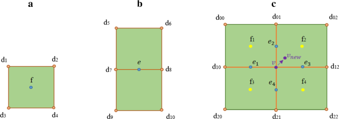

  

  Catmull-Clark subdivision scheme. a Finding the face point for each face. b Finding the edge point for each interior edge. c Computing the new position of vertex $v$ based on the face and edge points

  .

  $$\mathrm{f}=\frac{1}{4}\sum_{k=1}^{4}{\mathrm{d}}_{k},$$

  (9)
  $$e=\frac{1}{16}\left({d}_{5}+{d}_{6}+6*{d}_{7}+6*{d}_{8}+{d}_{9}+{d}_{10}\right) .$$

  (10)

• (2) Averaging step

  In the averaging step, the location of the vertex $v$ will be updated based on the face points (${\mathrm{f}}_{i}$) and edge points (${\mathrm{e}}_{i}$) around $v$ by

  $${v}_{new}=\frac{n-3}{n}*v+\frac{2}{n}*L+\frac{1}{n}*T,$$

  (11)

  where $n$ is the number of face or edge points around $v$; $L$ and $T$ are defined as

$$L=\frac{1}{n}\sum_{i=1}^{n}{\mathrm{e}}_{i},$$

(12)

$$T=\frac{1}{n}\sum_{i=1}^{n}{\mathrm{f}}_{i}.$$

(13)

Appendix 2: Non-Manifold Subdivision Surface Algorithm

Ying and Zorin (2001) defined the extended Loop subdivision algorithm to model non-manifold structures, which is described in the following.

T(v) is considered the set of all triangles of the mesh around vertex v (Fig. 19). Based on the definition in the previous section, vertex v is a manifold vertex if two favourite sequential triangles are inside T(v) and share one edge connected to v. This vertex can be either inside (interior vertex) or a boundary vertex. Additionally, an edge is named a manifold edge if it is shared by two triangles of the mesh (the manifold edge can be part of just one triangle if the edge is a boundary edge).

Fig. 19

Representation of T(v) (a set of triangles) around vertex v (centre vertex). a Representation of a manifold vertex v (blue vertex); two favourite sequential triangles inside T(v) share one edge connected to v. b Representation of a non-manifold vertex v (red vertex)

A non-manifold vertex and edge are named a singular vertex and edge, respectively. Considering M(v) are the largest set of triangles inside T(v) which consists of the specific triangles such that every pair of favourite sequential triangles around v share an edge (Fig.  20 shows T(v), which consists of M₁(v) and M₂(v)). It should be mentioned that the sets of triangles inside each M(v) can be either manifold or non-manifold. Also, non-manifold sets of triangles can be split into manifold sets. Therefore, each M(v) can be considered a combination of manifold segments, which are called Q(v); for example, M₁(v) and M₂(v) consist of one and three Q(v), respectively. Indeed, Q(v) (the manifold set of triangles around v) is the largest set of triangles such that all two sequential triangles of it share a manifold edge.

Fig. 20

T(v) consists of two parts (M₁(v) and M₂(v)); M₂(v) includes three-manifold parts, Q₂(v), Q₃(v) and Q₄(v), and M₁(v) has one manifold part, Q₁(v). The yellow edge represents the non-manifold edge which is shared between three edges

The singular vertex v is simple when it is part of a single M(v), and two singular edges should meet each other at v (all of the Q_(v)-manifold regions around v share edges); otherwise, it is a complex singular vertex (Fig. 21). For regular vertices, the standard Loop algorithm should be used. If the vertex is simple singular, the cubic B-spline subdivision algorithm (as mentioned in Sect. 2.4) should be used. Otherwise, the vertex is complex singular, and in most cases, a vertex can be fixed. Additionally, if the edge is singular, it should be subdivided at the midpoint, and if it is not singular, it should generally follow the regular Loop algorithm. For more information, please refer to Ying and Zorin (2001).

Fig. 21

Simple singular vertex (v) (orange vertex)

References

Börner JH, Bär M, Spitzer K (2015) Electromagnetic methods for exploration and monitoring of enhanced geothermal systems–a virtual experiment. Geothermics 55:78–87
Botsch M, Kobbelt L, Pauly M, Alliez P, Lévy B (2010) Polygon mesh processing. CRC Press, Cambridge
Brujic D, Ainsworth I, Ristic M (2011) Fast and accurate NURBS fitting for reverse engineering. Int J Adv Manuf Tech 54(5):691–700
Burns KL (1975) Analysis of geological events. J Int Assoc Math Geol 7(4):295–321
Cashman TJ (2010) NURBS-compatible subdivision surfaces
Catmull E, Clark J (1978) Recursively generated B-spline surfaces on arbitrary topological meshes. Comput Aided Des 10(6):350–355
Caumon G (2010) Towards stochastic time-varying geological modeling. Math Geosci 42(5):555–569
Caumon G, Lepage F, Sword CH, Mallet J-L (2004) Building and editing a sealed geological model. Math Geol 36(4):405–424
Caumon G, Collon-Drouaillet P, Carlier Le, de Veslud C, Viseur S, Sausse J (2009) Surface-based 3D modeling of geological structures. Math Geosci 41(8):927–945
Chen LQ, Liu D (2012) Research on the three-dimensional geological modeling based on subdivision surface modeling technology. Key Engineering Materials. Trans Tech Publ, pp 646–651
Cheng K-S, Wang W, Qin H, Wong K-Y, Yang H, Liu Y (2004) Fitting subdivision surfaces to unorganized point data using SDM. In: 12th Pacific Conference on Computer Graphics and Applications, 2004. PG 2004. Proceedings., 2004. IEEE, pp 16–24
Chui CK, Lai M-J, Lian J-a (2000) Algorithms for G1 connection of multiple parametric bicubic NURBS surfaces. Numer Algor 23(4):285–313
Corbett PWM, Geiger S, Borges L, Garayev M, Valdez C (2012) The third porosity systemunderstanding the role of hidden pore systems in well-test interpretation in carbonates. Pet Geosci 18(1):73–81
Dassi F, Perotto S, Formaggia L, Ruffo P (2014) Efficient geometric reconstruction of complex geological structures. Math Comput Simul 106:163–184
De Kemp EA (1999) Visualisation of complex geological structures using 3-D Bézier construction tools. Comput Geosci 25(5):581–597
de Kemp EA, Sprague KB (2003) Interpretive tools for 3-D structural geological modeling part I: bezier-based curves, ribbons and grip frames. GeoInformatica 7(1):55–71
de la Varga M, Schaaf A, Wellmann F (2019) GemPy 1.0: open-source stochastic geological modeling and inversion. Geoscient Mod Develop 12(1):1–32
DeRose T, Kass M, Truong T (1998) Subdivision surfaces in character animation. In: Proceedings of the 25th annual conference on Computer graphics and interactive techniques, pp 85–94
Deutsch CV (1997) FORTRAN programs for calculating connectivity of 3-D numerical models and for ranking multiple realisations. Submitted to Computers & Geosciences
Deveugle PEK, Jackson MD, Hampson GJ, Farrell ME, Sprague AR, Stewart J, Calvert CS (2011) Characterisation of stratigraphic architecture and its impact on fluid flow in a fluvial-dominated deltaic reservoir analog: upper Cretaceous Ferron Sandstone Member. Utah AAPG Bulletin 95(5):693–727
Doo D, Sabin M (1978) Behaviour of recursive division surfaces near extraordinary points. Comput Aided Des 10(6):356–360
Fisher TR, Wales RQ (1992) Three dimensional solid modeling of geo-objects using Non-Uniform Rational B-Splines (NURBS). Three-dimensional modeling with geoscientific information systems. Springer, Berlin, pp 85–105
Florez H, Manzanilla-Morillo R, Florez J, Wheeler MF (2014) Spline-based reservoir’s geometry reconstruction and mesh generation for coupled flow and mechanics simulation. Comput Geosci 18(6):949–967
Geiger S, Matthäi S (2014) What can we learn from high-resolution numerical simulations of single-and multi-phase fluid flow in fractured outcrop analogues? Geol Soci, London, Special Publications 374(1):125–144
Gjøystdal H, Reinhardsen JE, Åstebøl K (1985) Computer representation of complex 3-D geological structures using a new “solid modeling” technique. Geophys Prospect 33(8):1195–1211
Graham GH, Jackson MD, Hampson GJ (2015) Three-dimensional modeling of clinoforms in shallow-marine reservoirs: Part 1. Concepts and application. AAPG Bulletin 99(6):1013–1047
Graham GH, Jackson MD, Hampson GJ (2015) Three-dimensional modeling of clinoforms in shallow-marine reservoirs: Part 2 Impact on fluid flow and hydrocarbon recovery in fluvial-dominated deltaic reservoirs. AAPG Bulletin 99(6):1049–1080
Grinspun E, Schroder P (2001) Normal bounds for subdivision-surface interference detection. In: Proceedings Visualisation, 2001. VIS'01., 2001. IEEE, pp 333–570
Hassanpour MM, Pyrcz MJ, Deutsch CV (2013) Improved geostatistical models of inclined heterolithic strata for McMurray Formation, Alberta, Canada Geostatistical Models of Inclined Heterolithic Strata. Alberta AAPG Bulletin 97(7):1209–1224
Hoppe H, DeRose T, Duchamp T, Halstead M, Jin H, McDonald J, Schweitzer J, Stuetzle W (1994) Piecewise smooth surface reconstruction. In: Proceedings of the 21st annual conference on Computer graphics and interactive techniques. pp 295–302
Hughes M, DiMattia C, Lin MC, Manocha D (1996) Efficient and accurate interference detection for polynomial deformation. In: Proceedings Computer Animation'96, 1996. IEEE, pp 155–166
Jackson MD, Hampson GJ, Saunders JH, El-Sheikh A, Graham GH, Massart BYG (2014) Surface-based reservoir modelling for flow simulation. Geol Soci 387(1):271–292
Jackson MD, Percival JR, Mostaghimi P, Tollit BS, Pavlidis D, Pain CC, Gomes JL, El-Sheikh AH, Salinas P, Muggeridge AH (2015) Reservoir modeling for flow simulation by use of surfaces, adaptive unstructured meshes, and an overlapping-control-volume finite-element method. SPE Reserv Eval Eng 18(02):115–132
Jacquemyn C, Jackson MD, Hampson GJ (2019) Surface-based geological reservoir modelling using grid-free NURBS curves and surfaces. Math Geosci 51(1):1–28
Jaimez M, Kerl C, Gonzalez-Jimenez J, Cremers D (2017) Fast odometry and scene flow from RGB-D cameras based on geometric clustering. In: 2017 IEEE International Conference on Robotics and Automation (ICRA), 2017. IEEE, pp 3992–3999
Jones CB (1989) Data structures for three-dimensional spatial information systems in geology. Int J Geograph Infor Sys 3(1):15–31
Kälberer F, Nieser M, Polthier K (2007) Quadcover-surface parameterisation using branched coverings. Computer graphics forum, vol 3. Wiley, Hoboken, pp 375–384
Lane JM, Riesenfeld RF (1980) A theoretical development for the computer generation and display of piecewise polynomial surfaces. IEEE Trans Pattern Anal Mach Intell 1:35–46
Lavoué G, Dupont F, Baskurt A (2005) Subdivision surface fitting for efficient compression and coding of 3D models. In: Visual Communications and Image Processing, 2005. SPIE, pp 1159–1170
Lin M, Gottschalk S (1998) Collision detection between geometric models: A survey. In: Proc. of IMA conference on mathematics of surfaces. Citeseer, pp 602–608
Loop C (1987) Smooth subdivision surfaces based on triangles
Ma W, Ma X, Tso S-K, Pan Z (2004) A direct approach for subdivision surface fitting from a dense triangle mesh. Comput Aided Des 36(6):525–536
Ma X, Keates S, Jiang Y, Kosinka J (2015) Subdivision surface fitting to a dense mesh using ridges and umbilics. Comput Aid Geomet Design 32:5–21
Ma W, Ma X, Tso S-K, Pan Z (2002) Subdivision surface fitting from a dense triangle mesh. In: Geometric Modeling and Processing. Theory and Applications. GMP 2002. Proceedings. IEEE, pp 94–103
Mallet J-L (1997) Discrete modeling for natural objects. Math Geol 29(2):199–219
Mao Q, Liu S, Wang S, Ma X (2018) Surface fitting for quasi scattered data from coordinate measuring systems. Sensors 18(1):214
Marinov M, Kobbelt L (2005) Optimisation methods for scattered data approximation with subdivision surfaces. Graph Models 67(5):452–473
Kanai T MeshToSS: Converting Subdivision Surfaces from Dense Meshes. In: VMV, 2001. pp 325–332
Müller K, Reusche L, Fellner D (2006) Extended subdivision surfaces: Building a bridge between NURBS and Catmull-Clark surfaces. ACM Trans Graph (TOG) 25(2):268–292
Paluszny A, Matthäi SK, Hohmeyer M (2007) Hybrid finite element–finite volume discretisation of complex geologic structures and a new simulation workflow demonstrated on fractured rocks. Geofluids 7(2):186–208
Panozzo D, Puppo E, Tarini M, Pietroni N, Cignoni P (2011) Automatic construction of quad-based subdivision surfaces using fitmaps. IEEE Trans Visual Comput Graphics 17(10):1510–1520
Piegl L, Tiller W (1996) The NURBS book. Springer, Berlin
Pungotra H, Knopf GK, Canas R (2010) Merging multiple B-spline surface patches in a virtual reality environment. Comput Aided Des 42(10):847–859
Pyrcz MJ, Boisvert JB, Deutsch CV (2009) ALLUVSIM: a program for event-based stochastic modeling of fluvial depositional systems. Comput Geosci 35(8):1671–1685
Rossignac J, Cardoze D Matchmaker (1999) Manifold Breps for non-manifold r-sets. In: proceedings of the fifth ACM symposium on Solid modeling and applications, 1999. pp 31–41
Ruiu J, Caumon G, Viseur S (2016) Modeling channel forms and related sedimentary objects using a boundary representation based on non-uniform rational B-splines. Math Geosci 48(3):259–284
Sederberg TW, Zheng J, Bakenov A, Nasri A (2003) T-splines and T-NURCCs. ACM Trans Graph (TOG) 22(3):477–484
Sederberg TW, Cardon DL, Finnigan GT, North NS, Zheng J, Lyche T (2004) T-spline simplification and local refinement. ACM Trans Graph (TOG) 23(3):276–283
Sederberg TW, Finnigan GT, Li X, Lin H, Ipson H (2008) Watertight trimmed NURBS. ACM Trans Graph (TOG) 27(3):1–8
Sederberg TW, Zheng J, Sewell D, Sabin M (1998) Non-uniform recursive subdivision surfaces. In: Proceedings of the 25th annual conference on Computer Graphics and Interactive Techniques, 1998. pp 387–394
Severn A, Samavati F (2006) Fast intersections for subdivision surfaces. In: International conference on computational science and its applications. Springer, Berlin. pp 91–100
Shen J, Kosinka J, Sabin MA, Dodgson NA (2014) Conversion of trimmed NURBS surfaces to Catmull-Clark subdivision surfaces. Comput Aid Geomet Design 31(7–8):486–498
Sprague KB, De Kemp EA (2005) Interpretive tools for 3-D structural geological modelling part II: surface design from sparse spatial data. GeoInformatica 9(1):5–32
Suzuki H, Takeuchi S, Kanai T (1999) Subdivision surface fitting to a range of points. In: Proceedings. Seventh pacific conference on computer graphics and applications (Cat. No. PR00293), 1999. IEEE, pp 158–167
Theoharis T, Papaioannou G, Platis N, Patrikalakis NM (2008) Graphics and visualisation: principles & algorithms. CRC Press, Cambridge
Thiele ST, Jessell MW, Lindsay M, Ogarko V, Wellmann JF, Pakyuz-Charrier E (2016) The topology of geology 1: topological analysis. J Struct Geol 91:27–38
Urick B, Marussig B, Cohen E, Crawford RH, Hughes TJR, Riesenfeld RF (2019) Watertight boolean operations: a framework for creating CAD-compatible gap-free editable solid models. Comput Aided Des 115:147–160
Volino P, Thalmann NM (1994) Efficient self-collision detection on smoothly discretized surface animations using geometrical shape regularity. Computer graphics forum, vol 3. Wiley, Hoboken, pp 155–166
Vouga E, Goldman R (2007) Two blossoming proofs of the Lane-Riesenfeld algorithm. Computing 79(2):153–162
Warren J (1995) Subdivision methods for geometric design. Unpublished manuscript, November
Wellmann F, Caumon G (2018) 3-D Structural geological models: Concepts, methods, and uncertainties. Advances in Geophysics, vol 59. Elsevier, Armsterdam, pp 1–121
Wu X, Zheng J, Cai Y, Li H (2017) Variational reconstruction using subdivision surfaces with continuous sharpness control. Comput Visual Media 3(3):217–228
Ying L, Zorin D (2001) Nonmanifold subdivision. In: Proceedings Visualisation, 2001. VIS'01., 2001. IEEE, pp 325–569
Zehner B, Börner JH, Görz I, Spitzer K (2015) Workflows for generating tetrahedral meshes for finite element simulations on complex geological structures. Comput Geosci 79:105–117
Zhang X, Pyrcz MJ, Deutsch CV (2009) Stochastic surface modeling of deepwater depositional systems for improved reservoir models. J Petrol Sci Eng 68(1–2):118–134
Zorin D, Schröder P (2001) A unified framework for primal/dual quadrilateral subdivision schemes. Comput Aid Geomet Design 18(5):429–454
Zorin D (2000) Subdivision zoo. Subdivision for modeling and animation, Schröder, Peter and Zorin, Denis:65–104
Acknowledgements
We would like to thank our colleagues whose previous works motivated us to work on the topic, especially Prof. Guillaume Caumon, Dr. Pauline Collon, Prof. Leif Kobbelt, Prof. Matthew Jackson. This project has received funding from the European Institute of Innovation and Technology— Raw Materials—under grant agreements No. 16258 and No. 19004. It should be mentioned that the figures in this paper are rendered by Blender, which is an open-source 3D computer graphics software (http://www.blender.org/).
Funding
Open Access funding enabled and organized by Projekt DEAL. This article was funded by European Institute of Innovation and Technology— Raw Materials—under grant agreements No. 16258 and No. 19004.
Author information
Authors and Affiliations
Corresponding author
Ethics declarations
Conflict of interest
There are no conflicts of interest regarding this research.