
Abstract
Multimodal fusion is the idea of combining information in a joint representation of multiple modalities. The goal of multimodal fusion is to improve the accuracy of results from classification or regression tasks. This paper proposes a Bimodal Variational Autoencoder (BiVAE) model for audiovisual features fusion. Reliance on audiovisual signals in a speech recognition task increases the recognition accuracy, especially when an audio signal is corrupted. The BiVAE model is trained and validated on the CUAVE dataset. Three classifiers have evaluated the fused audiovisual features: Long-short Term Memory, Deep Neural Network, and Support Vector Machine. The experiment involves the evaluation of the fused features in the case of whether two modalities are available or there is only one modality available (i.e., cross-modality). The experimental results display the superiority of the proposed model (BiVAE) of audiovisual features fusion over the state-of-the-art models by an average accuracy difference \(\simeq \) 3.28% and 13.28% for clean and noisy, respectively. Additionally, BiVAE outperforms the state-of-the-art models in the case of cross-modality by an accuracy difference \(\simeq \) 2.79% when the only audio signal is available and 1.88% when the only video signal is available. Furthermore, SVM satisfies the best recognition accuracy compared with other classifiers.
1 Introduction
Within big data time, a massive amount of heterogeneous data are generated. These data are varied in modality, representation, and distribution. Integrating diverse data with different modalities to develop a more usable form of information is called multimodal data fusion. It is necessary to understand the distinction between multimodal and multi-channel data. Multi-channel data are the signals collected by multiple identical sensors, which means the signals are homogeneous. Explicitly, multi-channel data is not considered as a form of multimodal data.
Multimodal data fusion approaches are classified into four categories according to the level of fusion (Baltrušaitis et al., 2018): raw data fusion (also known as early fusion), decision fusion (also known as late fusion), hybrid fusion, and features fusion. Raw data fusion is a straightforward approach; it is just a concatenation among diverse data modalities to be the input into a machine learning algorithm. On the contrary, the decision fusion approach performs the fusion after taking a separate decision on each modality. In this approach, we can use the same predictive model for all modalities or different predictive models for each modality. Several decision fusion techniques may be used, such as voting schemes (Morvant et al., 2014), signal variance (Evangelopoulos et al., 2013), averaging (Shutova et al., 2016), and weighting based on channel noise (Potamianos et al., 2003). The hybrid data fusion approach is a combination of early fusion and late fusion approaches. It performs fusion on the decision using one of the decision fusion techniques, but the input of each predictive model is a concatenation of diverse modalities, and the predictive models must be different. The features fusion approach exploits the benefits of linear and non-linear correlations among the feature modalities to generate a single unified representation of those modalities.
Audiovisual speech recognition (AVSR) is one of the most common examples that emphasize the importance of multimodal data fusion in recognition tasks. Reliance on complementary data in a recognition task increases recognition accuracy, especially when one of the modalities is corrupted. Mainly, the need to AVSR model takes place when the audio signal is noisy while the visual signal is clean.
During the previous few years, neural networks have served in audio feature extraction (Sharma et al., 2020), visual feature extraction (Jogin et al., 2018), and performing a final classification at several applications of different disciplines (Bokade et al., 2020). Furthermore, deep learning models have played an essential role in capturing the intermodality features across different modalities and generating a unified representation of them (Gao et al., 2020). The recently developed deep neural networks for the AVSR task will be reviewed in the related work section.
The contribution of this paper is proposing a Bimodal Variational Autoencoder (BiVAE) for audiovisual features fusion that has the ability to:
-
Exploit the capabilities of VAE in smoothly learning the latent representations and generating new data to produce a strongly unified representation of the audiovisual feature.
-
Exceed the accuracy of other models in an audiovisual recognition task, especially at high levels of acoustic noise.
-
Perform a cross-modality, which considers the absence of some modalities during supervised training and testing phases. Wherefore, our proposed model can learn the joint representation even when some modalities are absent.
-
Generalize the performance with different feature extraction techniques for modalities and diverse classifiers.
This paper is structured as the following: Sect. 2 reviews the recent related work in AVSR. Section 3 explains an overview of the methods and models that have been used in the proposed architecture. Section 4 presents the proposed system. Sect. 5 discusses the experimental results. Section 6 introduces the conclusion.
2 Related work
Ngiam et al. (2011) proposed a bimodal deep autoencoder for AVSR. Their experiment included four schemes. All of the schemes were tested on the CUAVE database (Patterson et al., 2002). Furthermore, white Gaussian noise was added to a clean audio signal at 0 dB signal to noise ratio (SNR). They developed a restricted Boltzmann machine (RBM) (Hinton 2002) for audio-only speech recognition in the case of both clean audio and noisy audio. Also, they developed a deep autoencoder (Kramer 1991) for the lipreading task. Bimodal deep autoencoder could not exceed RBM recognition accuracy in both cases. Wherefore, they developed a bimodal deep autoencoder that was used with RBM. This combination achieved the most recognition accuracy in the case of noisy audio (82.2% against 79.6%), contrary to the case of clean audio (94.4% against 95.8%).
Rahmani et al. (2018) proposed an audiovisual feature fusion model based on a deep autoencoder. They used a Deep Neural Network-Hidden Markov Model hybrid (DNN-HMM) (Li et al., 2013) as a speech classifier. They aimed to overcome the inability of the bimodal deep autoencoder introduced by Ngiam et al. (2011) to perform a significant achievement with clean audio. They performed an adjustment of the ratio of contribution for each modality in the fusion process. Their feature fusion model was indeed able to surpass the bimodal deep autoencoder that has been proposed by Ngiam et al. (2011) in the case of clean audio (97.9% against 94.4%) and noisy audio (83.3% against 82.2%) on the CUAVE database. However, their adjustment was performed manually in over four attempts. Thus, it cannot be generalized.
Yang et al. (2017) proposed a Correlational Recurrent Neural Network (CorrRNN) model for multimodal fusion of temporal inputs. The main contribution of their work was a dynamic weighting mechanism. It permits the encoder to assign weights dynamically for each modality to adjust the contribution ratio of each one. The primary cause is to focus on the modality that has valuable information in a feature representation, especially when one of the modalities is corrupted by noise. The model was tested on the CUAVE database. The model achieved a significant superiority in the case of noisy audio (90.88%) while could not exceed the achievement of Rahmani et al. (2018) in the case of clean audio (96.11% against 97.9%).
Petridis et al. (2017) presented an end-to-end audiovisual speech recognition model using Bidirectional Long-short term memory (BLSTM) (Graves et al., 2005). This model can perform a lipreading task with multiple lip views. The model was tested on the OuluVS2 database (Anina et al., 2015). The end-to-end model outperformed the audio-only speech recognizer especially, at high levels of noise. However, the results showed the superiority of the lipreading classifier compared with the end-to-end model at high levels of noise.
Zhang et al. (2019) presented a bimodal Deep Feed-forward Sequential Memory Network (DFSMN) model for the AVSR task. Besides its ability to deal with noisy audio, it considers the issue of the absence of visual information during testing and deployment. They proposed a per-frame dropout regularization to deal with this issue. The model was evaluated on the NTCD-TIMIT database (Abdelaziz 2017). The bimodal DFSMN model achieved a phone error rate of 12.6% on clean conditions and an average phone error rate of 26.2% on all test sets (clean and noisy audio with various noise types at various SNRs) compared with DNN-HMM released by the Kaldi toolkit (Povey et al., 2011).
Yu et al. (2020) focused on the recognition of overlapped speech. In contrast to a traditional pipelined architecture for overlapped speech recognition, which contains explicit speech separation and recognition components, they proposed a streamlined and integrated AVSR system architecture. It has implicit speech enhancement and recognition components optimized consistently using the lattice-free Maximum Mutual Information (LF-MMI) discriminative criterion (Povey et al., 2016). The architecture was evaluated on the LRS2 dataset (Afouras et al., 2018). The architecture outperformed the audio-only baseline LF-MMI DNN system by up to 29.98% absolute in word error rate (WER) reduction.
3 Preliminaries
In this section, we will introduce an overview of the methods and algorithms used in our system. The section involves the explanation of Mel Frequency Cepstral Coefficients (MFCCs) algorithm and Gammatone Frequency Cepstral Coefficients (GFCC) algorithm for audio feature extraction, Histogram of Oriented Gradients (HOG) algorithm for face detection, Convolutional Neural Network (CNN) for visual feature extraction and lipreading, Variational Autoencoder (VAE) used in learning the mutual information between modalities, and Recurrent Neural Network (RNN), Deep Neural Network (DNN) and Support Vector Machine (SVM) classifiers.
3.1 Mel frequency cepstral coefficients (MFCCs)
MFCCs feature (Davis & Mermelstein, 1980) are widely used in the automatic speech recognition task. The job of MFCCs is to simulate how the human ear distinguishes the phonemes. It is evidenced by presenting its steps and the purpose of each step.
-
1.
Split the signal into short frames, where the audio signal does not change in a short time. Usually, the signal is framed into 20–40 ms frames. For a much shorter frame, there are no sufficient samples to obtain a valid spectral estimate. In contrast, the signal changes too much across the longer frame.
-
2.
Calculate the spectral density of the power spectrum for each frame using the Fast Fourier Transform (FFT) spectrum analyzer (Deery 2007). This calculation is motivated by the human cochlea; it vibrates depending on the frequency of the incoming sounds at different locations. The spectral density estimation plays the same role; it identifies the frequencies present in the frame.
-
3.
Apply the Mel-scale filter banks to the power spectrum to extract the frequency bands, then add the energy in each filter and take the logarithm of all filterbank energies. The Mel-scale filter imitates the non-linear human ear perception of sound; it discriminates low frequencies more than high frequencies.
-
4.
Calculate the Discrete Cosine Transform (DCT) (Ahmed et al., 1974) of the log filterbank energies. Because the filterbank energies are correlated due to the overlapping of filterbanks, the DCT decorrelates them. Out of the 26 DCT coefficients, only 13 are retained. Where the higher DCT coefficients reflect rapid changes in the energy of the filterbank and it turns out that these rapid changes degrade the output of ASR.
3.2 Gammatone frequency cepstral coefficients (GFCC)
GFCC can be stated as a biologically inspired MFCC modification that utilizes Gammatone (GT) filters with equivalent rectangular bandwidth (ERB) bands (Fathima & Raseena, 2013). GFCC computation is similar to MFCC. First, The audio signal is windowed into short frames, typically 10–50 ms. Then, the Gammatone filter bank (GT) is applied to the FFT of the signal. Finally, the log function and DCT are applied. The design of the GT filter considers the following characteristics: total filter bank bandwidth, ERB model (Lyon, Greenwood, or Glasberg and Moore), GT filter order n, and the number of filters N. The total cost of computing is nearly identical to that of the MFCC computation.
3.3 Histogram of oriented gradients (HOG)
HOG is a feature descriptor used widely in computer vision (Kim & Cho, 2014). It is applied in several pattern detection tasks such as object detection (Zaytseva et al., 2012), face detection (Shu et al., 2011), human detection (Dalal & Triggs, 2005), etc. It describes the texture of a rectangular block. It has achieved superior results in a facial detection task (Adnan et al., 2020). In the localized portions of an image, the technique counts occurrences of gradient orientation. The distribution of gradient directions is used as a feature in the HOG feature descriptor. An image’s gradients (x and y derivatives) are useful because the magnitude of gradients around edges and corners is high. The HOG feature descriptor can be estimated using algorithm 1.

3.4 Convolutional neural network (CNN)
CNN is one of the supervised deep learning models (Krizhevsky et al., 2017). It is used widely in image classification. There are two main reasons for its superiority in the image recognition task. First, no need for complex preprocessing; it takes the raw images directly. Second, it aims to automatically learn spatial and temporal features from low-level patterns to high-level patterns (Yamashita et al., 2018). Figure 1 illustrates the architecture of CNN, which consists of several convolutional layers, pooling layers, and fully connected layers.
-
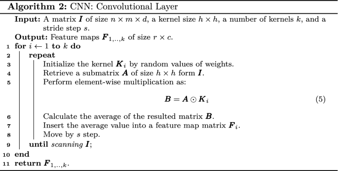
Convolutional Layer: is a primary component that performs a feature extraction using a linear operation (convolution operation) and non-linear operation (activation function) as demonstrated in algorithm 2.
-
Activation Function: is a non-linear function that transforms the output of linear operation such as convolution. Its purpose is to prevent the learning of trivial linear input combinations. There are several types of activation functions such as sigmoid, softmax, tanh, Rectified Linear Unit (ReLU), etc (Karlik & Olgac, 2011). In practice, ReLU is a commonly applied activation function.
-
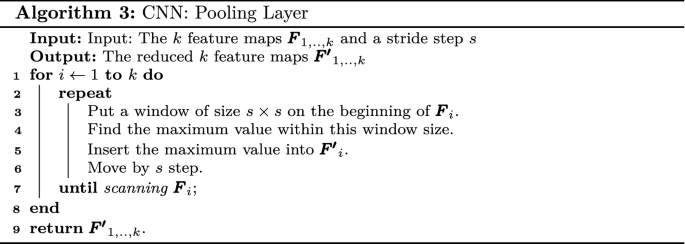
Pooling Layer: this down-sampling operation reduces the dimensionality of the feature map to the learnable parameters. There are two types of pooling operations called max pooling and average pooling. Max pooling is a commonly used pooling operation in practice, as illustrated in algorithm 3.
-
Fully Connected Layer: after the convolution and pooling operations sequence, the generated feature maps are flattened and passed to one or more connected dense layers. Its purpose is to calculate the probabilities of each class in classification tasks. An activation function follows each fully connected layer, such as ReLU. In contrast, the final layer (output layer) is followed by a different activation function, such as the softmax activation function in a multiclass classification task.


Convolutional neural network architecture

Autoencoder architecture
3.5 Variational autoencoder (VAE)
VAE is a deep generative model. It is one of the most popular approaches for unsupervised learning of complicated distributions (Kingma & Welling, 2014). In other words, VAE can be described as an autoencoder whose training is regularized. This regularization avoids overfitting and guarantees that the latent variables have sufficient characteristics. Consequently, a generative process is allowed (Doersch 2016).
The traditional autoencoder (AE) is an unsupervised learning model that is used mainly for a dimensionality reduction of data points (Hinton & Zemel, 1994). Figure 2 illustrates the architecture of the autoencoder. It consists of two neural networks: encoder network and decoder network. The encoder network maps the input data points \(x\in R^{d}\) into new features representation \(z\in R^{k}\) where \(k<d\), namely, latent variables. In contrast, the decoder network attempts to reconstruct approximately the data points from the latent variables such as \(\hat{x}= D(z)\). Using an iterative optimization process, the AE attempts to learn the best encoding decoding scheme that can keep the maximum amount of useful information when encoding, thus getting the minimum reconstruction error when decoding.
Suppose the encoder can organize the latent variables well during the training phase. In that case, the decoder can work as a data generator by selecting a point from the latent variables randomly and decode it to generate new data (Kingma & Welling, 2014). Indeed, there is no constraint in AE training that enforces it to regularize the points in the latent variables. A minor change has been done in the encoding-decoding processes to regularize the latent variables. The encoder encodes an input as a distribution over the latent variables to describe a probability distribution for each latent attribute, rather than encoding it as a single point to describe each latent state attribute. This modification is the objective of VAE. Figure 3 illustrates the difference in the encoding-decoding behavior between AE and VAE. The term “variational” is derived from the close relationship between the regularization and the variational inference in statistics (Zhu et al., 2014). Variational inference is widely used to approximate distributions in complex latent variables (Ranganath et al., 2014).

The difference between autoencoder (AE) and variational autoencoder (VAE)
VAE architecture consists of a probabilistic encoder defined by p(z|x) and a probabilistic decoder defined by p(x|z) given by a fixed prior p(z). To infer good values from the latent variables given the observed data, the calculation of the posterior p(z|x) is given by:
where x is called the evidence. It is calculated by marginalizing out the latent variables as:
Unfortunately, for all configurations of latent variables, this integral takes exponential time to calculate as it needs to be evaluated. Therefore, this posterior distribution needs to be estimated. Variational inference approximates the posterior with a family of distributions \({q}_\lambda (z|x)\). The variational parameter \(\lambda \) indexes the family of distributions. Kullback-Leibler divergence (KL) (Joyce 2011) is used for knowing how well a variational posterior q(z|x) approximates the true posterior p(z|x), which measures the lost information when using q to approximate p.
The joint representation of the model p(x, z) can be written as:
The goal is to minimize this divergence by obtaining the optimal variational parameters \(\lambda \) that minimize it. In this way, the optimal estimated posterior is given by:
The main idea of the variational autoencoder (VAE) is to impose a probability distribution (usually Gaussian) on the latent variables and learns the distribution. Therefore, the distribution of the decoder outputs matches that of the observed data. Afterward, this distribution is sampled to generate new data.
3.6 Deep neural network (DNN)
DNN is a multi-layer artificial neural network (Goodfellow et al., 2016). It consists of an input layer, output layer, and one or more hidden layers. An activation function follows each layer. DNN is a feedforward network that transfers data from the input layer to the output layer without looping back. It uses the backpropagation algorithm to propagate the error back to adjust the weights and bias of the network. Figure 4 demonstrates the basic architecture of DNN.

Deep neural network architecture
3.7 Recurrent neural network (RNN)
RNN is a neural network that releases dynamic information in sequential data through hidden layer nodes with periodical connections (Rumelhart et al., 1986). On the contrary to other forward neural networks, RNN can preserve a context state and even store, learn, and express related information in the context windows of any length and classify sequential data. Moreover, RNN extends in space and time sequences, unlike the traditional neural networks. The hidden layers of the current and the next moment are interrelated, as presented in Fig. 5. Furthermore, RNN is extensively used in scenarios related to sequences, such as sentences consisting of words (Tarwani & Edem, 2017), videos consisting of image frames (Lakshmi et al., 2020), and audio consisting of clips (Amberkar et al., 2018).
There are three common types of RNNs: Long-short Term Memory (LSTM) (Hochreiter & Schmidhuber 1997), Gated Recurrent Units (GRUs) (Cho et al., 2014), and Bidirectional RNNs either with LSTM as Bidirectional Long-short Term Memory (BLSTM) (Thireou & Reczko, 2007) or with GRUs as Bidirectional Gated Recurrent Units (BGRUs) (Faruk et al., 2020). All of the types aim to avoid the vanishing gradient problem with little difference in a mechanism.

Recurrent neural network architecture
3.8 Support vector machine (SVM)
SVM was presented by Cortes and Vapnik (1995). It is one of the supervised learning algorithms that solve both classification and regression problems. It performs classification by finding the hyper-plane that differentiates the two classes very well. It maximizes the distances between the nearest data point of each class and hyper-plane to decide the right hyper-plane. This distance is namely “Margin”. It considers linear and non-linear data by using the so-called “kernel trick,” as presented in Fig. 6. The Gaussian kernel is used in this work; it is the most commonly utilized kernel in practice.

Linear and non-linear classification by support vector machine
4 Proposed system
The details of the proposed system will be introduced in this section. The proposed system consists of three phases. The first phase includes data preprocessing for both audio and visual signals. The second phase covers the performing of audiovisual features fusion using our proposed model BiVAE, which is our main contribution. The last phase involves audiovisual speech recognition using the three classifiers. The general structure of the proposed system is demonstrated in Fig. 7.

The proposed system structure
4.1 Data preprocessing
4.1.1 Audio signal
In this section, the steps of preparing an audio signal for speech recognition will be illustrated. The audio preprocessing phase involves performing audio alignment with video to ensure they have the same length, adding noise, and extracting MFCC and GFCC features from the audio signal. In the following, the details of each step will be demonstrated.
-
Audio Alignment with Video: this step means extracting the audio from a video to guarantee the same length of both.
-
Adding Noise: the main focus of this step is making a distortion in the audio signal. A copy from the extracted clean audio signal has been taken, and then a noise has been added with various signal-to-noise-ratio (SNR). SNR is a ratio of the signal power to the noise power. In this work, a White Gaussian noise has been added with several values of SNR [15 dB, 10 dB, 5 dB, 0 dB, -5 dB, -10 dB, -15 dB]. This noisy signal will be used for measuring the robustness of the proposed system in recognizing a speech from a distorted signal and emphasizing the effect of utilizing the complementary visual signal in increasing the accuracy of speech recognition when an audio signal is corrupted.
-
Audio Feature Extraction: 13 MFCC features and 13 GFCC features are extracted from each signal frame for both clean and noisy signals. This work performed the feature extraction process using window length equal 0.025s, “Hamming” window function, window step equal 0.01s, FFT size equal 512, and sample rate equal 16 kHZ. For each sample file, a feature matrix with \(\hbox {n} \times 13\) dimensions is generated, where n is the number of frames per sample, the same as GFCC features matrix. Zero padding is necessary post-processing as a result of a different number of frames in each sample.
4.1.2 Visual signal
This sub-phase aims to extract the visual features from each video stream. The steps of achieving this aim will be demonstrated in this section. The visual signal preprocessing task consists of framing, face detection, mouth segmentation, frame stretching, and visual features extraction. Each step will be described in full below.
-
Framing: any video stream consists of many frames. To extract information from the video stream, splitting it into its frames must be the initial step.
-
Face Detection: at this step, the human face must be detected from the scene. For each frame, the face is detected using the HOG feature descriptor because of its superior results compared with other algorithms (Adnan et al., 2020).
-
Mouth Segmentation: in a lipreading task, a mouth is a region of interest (ROI). To detect this ROI, the facial landmarks detector that was introduced by Kazemi and Sullivan (2014) has been used. The pre-trained facial landmark detector is used to estimate the location of 68 (x, y)-coordinates that map to facial structures on the face. It was trained on the iBUG 300-W dataset (Sagonas et al., 2013). Figure 8 illustrates the coordinates of the facial landmarks. Depending on the ROI coordinates, the mouth is cropped.
-
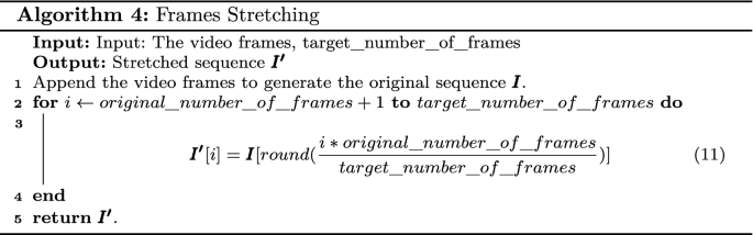
Frames Stretching: the used data contains multiple images per instance with a variable length for each instance. the aim of this step is to prepare the data for the visual features extraction step. Due to the CNN nature of taking a single image per instance as input, the sequence of images per instance is appended to generate a single image with equal width and height. The frames stretching method introduced in Garg et al. (2016) is utilized to unify the dimensions of the generated images for all instances. Frames stretching means filling the missing location in the generated sequence by the nearest image in the original sequence according to the following algorithm 4.
-
Visual Features Extraction: CNN is a commonly used model for image feature extraction in the image classification task. Constructing a CNN model from scratch to get strong features needs a lot of data and therefore requires huge computation resources; this consumes a lot of time and cost. To avoid this problem, we used a pre-trained model on a huge amount of data in a similar task. That is called transfer learning. In other words, transfer learning means storing the weights acquired while solving one task and applying it to a different but related task. VGGFace2 model is a pre-trained model for face recognition (Cao et al., 2018). It was trained on 3.31 M images for 9,131 identities. It satisfied an error reduction rate by 6.7 compared with the VGGFace model (Parkhi et al., 2015) and can perform face recognition across different poses and ages. In this work, the VGGFace2 model is utilized to get strong visual features.


The 68 facial landmarks coordinates (Sagonas et al., 2013)
4.2 Features fusion using BiVAE
In this phase, a multimodal features fusion task is performed based on the VAE. Intuitively, the primary principle of VAE is that it embeds the x input rather than a point into a distribution. Then, a random sample z is taken from the distribution rather than directly generated from the encoder. The VAE decoder works as a data generator, unlike the standard AE used for dimensional reduction. The capabilities of VAE in learning smooth latent representations and generating new data have been exploited for generating a unified representation from multimodal data. BiVAE is a proposed bimodal model for feature fusion. Figure 9 shows the structure of the proposed BiVAE, which is used for audiovisual features fusion. The proposed structure consists of five hidden layers. The three middle layers share bimodal information. The audio features vector and visual features vector are multiplied by \(W_{L}^{1}\) and \(W_{R}^{1}\) weight matrices, respectively. Then, they are passed through the non-linear ReLU function separately to form the first abstraction layers of audio (\(h_{A}^{1}\)) and visual (\(h_{V}^{1}\)). Next, the abstraction layers \(h_{A}^{1}\) and \(h_{V}^{1}\) are multiplied by \(W_{L}^{3}\) and \(W_{R}^{3}\) and concatenated. By performing the ReLU function to the concatenated matrices, the first mutual layer is formed \(h_{AV}^{1}\). At the next step, \(h_{AV}^{1}\) is multiplied by \(W^{5}\) to form the latent variables.
VAE forces latent variables to become normally distributed; this happens by creating two vectors: vector of means and variances. The values from a normal distribution are sampled to generate well-organized latent variables. The latent variables contain the mutual information from the two modalities, being used as an input in the AVSR task. The described steps are continued layer by layer on the decoding side by applying the related weight matrices to the layers involved until reconstructing both the audio and the visual inputs. The greedy layer-wise pretraining technique (Bengio et al., 2007) is utilized for the BiVAE training process to put the network at an appropriate initial point before the final training process and prevent the vanishing gradient problem. The greedy layer-wise pretraining technique is defined as iterative network training, starting with shallow network architecture and adding a new layer one by one iteratively. The fine-tuning stage is done to minimize the loss function.

Bimodal variational autoencoder (BiVAE) structure for audiovisual features fusion (A: Audio, V: Visual, and AV: Audiovisual)
4.3 AVSR task
In this phase, The three classifiers (DNN, RNN, and SVM) perform the AVSR task. This phase aims to assess the efficiency of the latent variables generated by BiVAE in the AVSR task and measure the benefit of exploiting the visual information in speech recognition tasks, especially in the case of the corrupted audio signal. The accuracy of speech recognition based on the audiovisual features indicates the ability of the BiVAE to learn the non-linear correlations between the two signals and generate a single unified representation from the two modalities.
5 Experimental results and discussion
In this section, the performed experiment details will be introduced, and the achieved results will be discussed. The experiment contains three stages:
-
1.
Audio Speech Recognition (ASR) task.
-
2.
Lipreading task.
-
3.
AVSR task based on BiVAE.
The stages of the experiment have been conducted on the CUAVE database. The results of the third stage, which are our main target, have been compared with the results of other state-of-the-art models. The aim of this comparison is to emphasize the importance of exploiting the visual signal in a speech recognition task, especially with corrupted audio. Furthermore, the performance of BiVAE has been compared with other models: Bimodal + Audio RBM (Ngiam et al., 2011), DNN-IV (Rahmani et al., 2018), and CorrRNN (Yang et al., 2017) in terms of accuracy in the AVSR task. Table 1 shows the specifications of the experimental environment. The implementation of the proposed model has been done using python and Keras API.
5.1 Data description
The CUAVE database (Patterson et al., 2002) is audiovisual. It includes isolated digits from 0 to 9 and connected digits. They were pronounced by 36 speakers (19 males and 17 females). In this database, both the individual speakers and the speaker pairs are involved with frontal and profile views. In this experiment, the speaker pairs and the profile views of the speakers are excluded. The total number of used utterances in this experiment is 2880 utterances (80 per speaker).
5.2 ASR tasks results
In this stage, the speech recognition task is performed based on audio signal only. FFMPEG tools is used to extract the audio from audiovisual data to perform an audio alignment with video. The audio files is read using read function in Soundfile module that supports any audio file format. White Gaussian noise is added to the clean audio with several values of SNR [15 dB, 10 dB, 5 dB, 0 dB, -5 dB, -10 dB, -15 dB]. The MFCCs features are extracted from both the clean and noisy audio using the mfcc module in the python_speech_features package that supports any sampling rates. Similarly, GFCCs features are extracted from both the clean and noisy audio using the gfcc module in the spafe.features package. LSTM, DNN, and SVM classifiers perform ASR tasks on clean and noisy audio separately with MFCC and GFCC features. The accuracy of the ASR tasks over five independent is recorded for each classifier. Tables 2, 3 and 4 show the difference in performance between MFCC and GFCC features in terms of accuracy over the three classifiers.
5.3 Lipreading task results
In this stage, the speech recognition task is performed based on visual signal only. In the beginning, the video frames are captured using VideoCapture function in OpenCV module that supports any video format. Then, ROI is segmented based on the coordinates of the facial landmarks. Afterward, the frames stretching process is performed with \(7\times 7\) frames in the single image for each video. Finally, the generated images from the stretching process are resized into \(224\times 224\times 3\) to satisfy the requirements of the utilized pre-training model. The pre-trained VGGFace2 model is used for the lipreading task. The last fully connected layer is replaced, which now classifies ten classes using the softmax activation function. Then, the fully connected layers are re-trained on our task. Table 5 shows the average and standard deviation of the performance metrics for the lipreading task over five independent runs. Tables 2, 3 and 4 show the difference in performance between MFCC and GFCC features in terms of accuracy over the three classifiers.

The performance of LSTM classifier for AVSR tasks based on MFCC and GFCC separately

The performance of DNN classifier for AVSR tasks based on MFCC and GFCC separately

The performance of SVM classifier for AVSR tasks based on MFCC and GFCC separately
5.4 AVSR tasks results
In this stage, the speech recognition task is performed based on audio and visual signals. The experiment considers whether both modalities are available or only a single modality is available during the supervised training and test. BiVAE is used for feature learning. It takes audio and visual features to compute the latent variables. The experiment involves visual features fusion with MFCC and GFCC audio features separately. Moreover, a cross-modality experiment is performed for both types of audio features. When computing the latent variables in the case of cross-modality, we set the value of the other modality to zero. Table 6 shows the assigned optimal values of BiVAE hyper-parameters. These values are determined using the grid search algorithm (Shekar & Dagnew, 2019).
LSTM, DNN, and SVM are used for the AVSR task. They take the latent variables as input and recognize the pronounced word. The AVSR tasks are performed on clean and noisy audio, once with fused MFCC and visual features and another time with fused GFCC and visual features over the three classifiers. Similar to ASR, the accuracy of the AVSR tasks over five independent runs is recorded for each classifier. Tables 7, 8 and 9 show the performance of AVSR with fused MFCC and visual features and with fused GFCC and visual features over the three classifiers in terms of accuracy. Moreover, Figs. 10, 11 and 12 illustrate the ability of BiVAE to enhance the recognition accuracy of the speech through integrating the audio signal with the visual signal. The results in Tables 2, 2, 4, 7, 8, 9, and Figs. 10, 11 and 12 illustrate the following:
-
1.
The superiority of our proposed fusion model in the AVSR task compared with the results of the ASR task, especially when the audio signal is corrupted, by the average accuracy improvement up to \(\simeq \) 23.33%, 36.81%, and 33.83% over LSTM, DNN, and SVM, respectively.
-
2.
Although the MFCC outperforms the GFCC in ASR, their performances are somewhat similar in AVSR, especially in DNN and SVM results; That means the ability of BiVAE to generalize its performance with different feature extraction techniques.
-
3.
The SVM classifier exceeds the LSTM and DNN in terms of speech recognition accuracy for both ASR and AVSR tasks.
Furthermore, BiVAE outperforms the state-of-the-art models. Table 10 shows the difference in terms of accuracy between our model BiVAE, Bimodal + Audio RBM model (Ngiam et al., 2011), DNN-IV model model (Rahmani et al., 2018), and CorrRNN model (Yang et al., 2017) in clean and noisy audio based on MFCC features.
Moreover, BiVAE outperforms the state-of-the-art models in both cases (i.e., The absence of the acoustic features or the absence of the visual features in the supervised train and test processes). Table 11 shows the difference in terms of accuracy between our model BiVAE, Bimodal + Audio RBM model (Ngiam et al., 2011), and CorrRNN model (Yang et al., 2017) based on MFCC features in the case of cross modality.
As illustrated in Tables 10 and 11, BiVAE outperforms the sate-of-the-art models with DNN and SVM classifiers in the case of multimodal and cross-modality. Regardless BiVAE with LSTM classifier in the case of multimodal, it outperforms the Bimodal + Audio RBM model and CorrRNN model for both clean and noisy audio. In contrast, it outperforms the DNN-IV model for noisy audio. In the case of cross-modality, it exceeds the Bimodal + Audio RBM model when the only video signal is available.
6 Conclusion
Multimodal fusion of data, one of the most trendy research points, was studied in this paper. The audiovisual speech recognition task was taken as an example of multimodal data.
This paper proposed a bimodal model for features fusion based on the generative model VAE, named, BiVAE. The ability of VAE to deal with complex data distributions through the variational inference indicated the strength and efficiency of the generated unified representation in the speech recognition task, especially at high levels of acoustic noise. Our system consists of three phases: data preprocessing for audio and visual signals, features fusion, and fused features evaluation through the speech recognition task.
The experiment was concerned with measuring the performance of the AVSR model based on BiVAE against the ASR model, especially when the audio signal was corrupted, based on two audio features extraction techniques, namely, MFCC and GFCC, and over the three classifiers LSTM, DNN, and SVM. Furthermore, it was concerned with measuring the performance of BiVAE against the state-of-the-art features fusion models through the AVSR task over the three classifiers. The experimental results showed the suppression of the AVSR model based on BiVAE in speech recognition compared with the ASR model by an average accuracy difference up to \(\simeq \) 23.33%, 36.81%, and 33.83% over LSTM, DNN, and SVM, respectively. Moreover, although the MFCC outperformed the GFCC in ASR, their performances were somewhat similar in AVSR, especially in DNN and SVM results; that means the ability of BiVAE to generalize its performance with different feature extraction techniques. Besides, the SVM classifier exceeded the LSTM and DNN in terms of speech recognition accuracy for both ASR and AVSR tasks. Furthermore, our proposed model with the three classifiers outperformed the state-of-the-art models, especially in the case of noisy audio, which means the ability of BiVAE to generalize its performance with different classifiers. BiVAE exceeded the state-of-the-art models in the AVSR task by an average accuracy difference \(\simeq \) 3.28% and 13.28% for clean and noisy, respectively. Additionally, BiVAE outperformed the state-of-the-art models in the case of cross-modality by an accuracy difference \(\simeq \) 2.79% when the only audio signal is available and 1.88% when the only video signal is available.
We suggest designing online and incremental multimodal deep learning models for real-time multimodal data fusion for future research.
References
Abdelaziz, A. H. (2017). Ntcd-timit: A new database and baseline for noise-robust audio-visual speech recognition. In: INTERSPEECH (pp. 3752–3756).
Adnan, S., Ali, F., & Abdulmunem, A. A. (2020). Facial feature extraction for face recognition. Journal of Physics: Conference Series, IOP Publishing, 1664, 012050.
Afouras, T., Chung, J. S., Senior, A., Vinyals, O., & Zisserman, A. (2018). Deep audio-visual speech recognition. IEEE Transactions on Pattern Analysis and Machine Intelligence. https://doi.org/10.1109/TPAMI.2018.2889052
Ahmed, N., Natarajan, T., & Rao, K. R. (1974). Discrete cosine transform. IEEE Transactions on Computers, 100(1), 90–93.
Amberkar, A., Awasarmol, P., Deshmukh, G., & Dave, P. (2018). Speech recognition using recurrent neural networks. In: 2018 international conference on current trends towards converging technologies (ICCTCT) (pp. 1–4). IEEE.
Anina, I., Zhou, Z., Zhao, G., & Pietikäinen, M. (2015). Ouluvs2: A multi-view audiovisual database for non-rigid mouth motion analysis. In 2015 11th IEEE international conference and workshops on automatic face and gesture recognition (FG) (vol. 1, pp. 1–5). IEEE.
Baltrušaitis, T., Ahuja, C., & Morency, L. P. (2018). Multimodal machine learning: A survey and taxonomy. IEEE Transactions on Pattern Analysis and Machine Intelligence, 41(2), 423–443.
Bengio, Y., Lamblin, P., Popovici, D., & Larochelle, H. (2007). Greedy layer-wise training of deep networks. In Advances in neural information processing systems (pp. 153–160).
Bokade, R., Navato, A., Ouyang, R., Jin, X., Chou, C. A., Ostadabbas, S., & Mueller, A. V. (2020). A cross-disciplinary comparison of multimodal data fusion approaches and applications: Accelerating learning through trans-disciplinary information sharing. In Expert Systems with Applications (pp. 113885).
Cao, Q., Shen, L., Xie, W., Parkhi, O. M., & Zisserman, A. (2018). Vggface2: A dataset for recognising faces across pose and age. In 2018 13th IEEE international conference on automatic face and gesture recognition (FG 2018) (pp. 67–74). IEEE
Cho, K., Van Merriënboer, B., Gulcehre, C., Bahdanau, D., Bougares, F., Schwenk, H., & Bengio, Y. (2014). Learning phrase representations using rnn encoder-decoder for statistical machine translation. In Proceedings of the 2014 conference on empirical methods in natural language processing (EMNLP), association for computational linguistics, Doha, Qatar (pp. 1724–1734). https://doi.org/10.3115/v1/D14-1179, https://aclanthology.org/D14-1179
Cortes, C., & Vapnik, V. (1995). Support-vector networks. Machine Learning, 20(3), 273–297.
Dalal, N., Triggs, B. (2005). Histograms of oriented gradients for human detection. In 2005 IEEE computer society conference on computer vision and pattern recognition (CVPR05) (Vol. 1, pp. 886–893). IEEE.
Davis, S., & Mermelstein, P. (1980). Comparison of parametric representations for monosyllabic word recognition in continuously spoken sentences. IEEE Transactions on Acoustics, Speech, and Signal Processing, 28(4), 357–366.
Deery, J. S. (2007). The ‘real’ history of real-time spectrum analyzers a 50-year trip down memory lane. Sound and Vibration, 41, 54–59.
Doersch, C. (2016). Tutorial on variational autoencoders. arXiv:160605908
Evangelopoulos, G., Zlatintsi, A., Potamianos, A., Maragos, P., Rapantzikos, K., Skoumas, G., & Avrithis, Y. (2013). Multimodal saliency and fusion for movie summarization based on aural, visual, and textual attention. IEEE Transactions on Multimedia, 15(7), 1553–1568.
Faruk, A., Faraby, H. A., Azad, M. M., Fedous, M. R., & Morol, M. K. (2020). Image to Bengali caption generation using deep cnn and bidirectional gated recurrent unit. In 2020 23rd international conference on computer and information technology (ICCIT) (pp. 1–6).
Fathima, R., & Raseena, P. (2013). Gammatone cepstral coefficient for speaker identification. International Journal of Advanced Research in Electrical, Electronics and Instrumentation Engineering, 2(1), 540–545.
Gao, J., Li, P., Chen, Z., & Zhang, J. (2020). A survey on deep learning for multimodal data fusion. Neural Computation, 32, 829–864.
Garg, A., Noyola, J., Bagadia, S. (2016). Lip reading using cnn and lstm. Technical report, Stanford University, CS231 n project report.
Goodfellow, I., Bengio, Y., & Courville, A. (2016). Deep learning. MIT Press. http://www.deeplearningbook.org
Graves, A., Fernández, S., & Schmidhuber, J. (2005). Bidirectional lstm networks for improved phoneme classification and recognition. In International conference on artificial neural networks (pp. 799–804). Springer.
Hinton, G. E. (2002). Training products of experts by minimizing contrastive divergence. Neural Computation, 14(8), 1771–1800.
Hinton, G. E., & Zemel, R. S. (1994). Autoencoders, minimum description length and helmholtz free energy. In Advances in neural information processing systems (pp. 3–10).
Hochreiter, S., & Schmidhuber, J. (1997). Long short-term memory. Neural Computation, 9(8), 1735–1780.
Jogin, M., Madhulika, M., Divya, G., Meghana, R., Apoorva, S., et al. (2018). Feature extraction using convolution neural networks (cnn) and deep learning. In 2018 3rd IEEE international conference on recent trends in electronics, information and communication technology (RTEICT) (pp. 2319–2323). IEEE.
Joyce, J. M. (2011). Kullback–Leibler divergence (pp. 720–722). Berlin: Springer. https://doi.org/10.1007/978-3-642-04898-2_327.
Karlik, B., & Olgac, A. V. (2011). Performance analysis of various activation functions in generalized mlp architectures of neural networks. International Journal of Artificial Intelligence and Expert Systems, 1(4), 111–122.
Kazemi, V., & Sullivan, J. (2014). One millisecond face alignment with an ensemble of regression trees. In Proceedings of the IEEE conference on computer vision and pattern recognition (pp. 1867–1874).
Kim, S., & Cho, K. (2014). Fast calculation of histogram of oriented gradient feature by removing redundancy in overlapping block. J Inf Sci Eng, 30(6), 1719–1731.
Kingma, D. P, & Welling, M. (2014). Auto-encoding variational bayes. CoRR arXiv:1312.6114
Kramer, M. A. (1991). Nonlinear principal component analysis using autoassociative neural networks. AIChE Journal, 37(2), 233–243.
Krizhevsky, A., Sutskever, I., & Hinton, G. E. (2017). Imagenet classification with deep convolutional neural networks. Communications of the ACM, 60(6), 84–90.
Lakshmi, K. P., Solanki, M., Dara, J. S., & Kompalli, A. B. (2020). Video genre classification using convolutional recurrent neural networks. International Journal of Advanced Computer Science and Applications. https://doi.org/10.14569/IJACSA.2020.0110321.
Li, L., Zhao, Y., Jiang, D., Zhang, Y., Wang, F., Gonzalez, I., Valentin, E., & Sahli, H. (2013). Hybrid deep neural network–hidden markov model (dnn-hmm) based speech emotion recognition. In 2013 Humaine association conference on affective computing and intelligent interaction (pp. 312–317). IEEE.
Morvant, E., Habrard, A., & Ayache, S. (2014). Majority vote of diverse classifiers for late fusion. In Joint IAPR international workshops on statistical techniques in pattern recognition (SPR) and structural and syntactic pattern recognition (SSPR) (pp 153–162). Springer.
Ngiam, J., Khosla, A., Kim, M., Nam, J., Lee, H., & Ng, A. Y. (2011). Multimodal deep learning. In L. Getoor & T. Scheffer (Eds.), ICML (pp. 689–696). Omnipress. http://dblp.uni-trier.de/db/conf/icml/icml2011.html#NgiamKKNLN11.
Parkhi, O. M., Vedaldi, A., & Zisserman, A. (2015). Deep face recognition. In British machine vision conference (pp. 41.1–41.12,). BMVA Press. https://doi.org/10.5244/C.29.41
Patterson, E. K., Gurbuz, S., Tufekci, Z., & Gowdy, J. N. (2002). Cuave: A new audio-visual database for multimodal human-computer interface research. In 2002 IEEE international conference on acoustics, speech, and signal processing (Vol. 2, pp. II–2017). IEEE.
Petridis, S., Li, Z., & Pantic, M. (2017). End-to-end visual speech recognition with lstms. In 2017 IEEE international conference on acoustics, speech and signal processing (ICASSP) (pp 2592–2596). IEEE.
Potamianos, G., Neti, C., Gravier, G., Garg, A., & Senior, A. W. (2003). Recent advances in the automatic recognition of audiovisual speech. Proceedings of the IEEE, 91(9), 1306–1326.
Povey, D., Ghoshal, A., Boulianne, G., Burget, L., Glembek, O., Goel, N., Hannemann, M., Motlicek, P., Qian, Y., Schwarz, P., et al. (2011). The kaldi speech recognition toolkit. In IEEE 2011 workshop on automatic speech recognition and understanding, IEEE Signal Processing Society, CONF.
Povey, D., Peddinti, V., Galvez, D., Ghahremani, P., Manohar, V., Na, X., Wang, Y., & Khudanpur, S. (2016). Purely sequence-trained neural networks for asr based on lattice-free mmi. In Interspeech (pp. 2751–2755).
Rahmani, M. H., Almasganj, F., & Seyyedsalehi, S. A. (2018). Audio-visual feature fusion via deep neural networks for automatic speech recognition. Digital Signal Processing, 82, 54–63.
Ranganath, R., Gerrish, S., & Blei, D. (2014). Black box variational inference. In Artificial intelligence and statistics, PMLR (pp. 814–822).
Rumelhart, D. E., Hinton, G. E., & Williams, R. J. (1986). Learning representations by back-propagating errors. Nature, 323(6088), 533–536.
Sagonas, C., Tzimiropoulos, G., Zafeiriou, S., & Pantic, M. (2013). 300 faces in-the-wild challenge: The first facial landmark localization challenge. In Proceedings of the IEEE international conference on computer vision workshops (pp. 397–403).
Sharma, G., Umapathy, K., & Krishnan, S. (2020). Trends in audio signal feature extraction methods. Applied Acoustics, 158, 107020.
Shekar, B., & Dagnew, G. (2019). Grid search-based hyperparameter tuning and classification of microarray cancer data. In 2019 second international conference on advanced computational and communication paradigms (ICACCP) (pp. 1–8). IEEE.
Shu, C., Ding, X., & Fang, C. (2011). Histogram of the oriented gradient for face recognition. Tsinghua Science and Technology, 16(2), 216–224.
Shutova, E., Kiela, D., & Maillard, J. (2016). Black holes and white rabbits: Metaphor identification with visual features. In Proceedings of the 2016 conference of the north american chapter of the association for computational linguistics: human language technologies (pp. 160–170).
Tarwani, K. M., & Edem, S. (2017). Survey on recurrent neural network in natural language processing. International Journal of Engineering Trends and Technology, 48, 301–304.
Thireou, T., & Reczko, M. (2007). Bidirectional long short-term memory networks for predicting the subcellular localization of eukaryotic proteins. IEEE/ACM Transactions on Computational Biology and Bioinformatics, 4(3), 441–446.
Yamashita, R., Nishio, M., Do, R. K. G., & Togashi, K. (2018). Convolutional neural networks: An overview and application in radiology. Insights into Imaging, 9(4), 611–629.
Yang, X., Ramesh, P., Chitta, R., Madhvanath, S., Bernal, E. A., & Luo, J. (2017). Deep multimodal representation learning from temporal data. In Proceedings of the IEEE conference on computer vision and pattern recognition (pp. 5447–5455).
Yu, J., Zhang, S. X., Wu, J., Ghorbani, S., Wu, B., Kang, S., Liu, S., Liu, X., Meng, H., & Yu, D. (2020). Audio-visual recognition of overlapped speech for the lrs2 dataset. In ICASSP 2020–2020 IEEE international conference on acoustics, speech and signal processing (ICASSP) (pp 6984–6988). IEEE.
Zaytseva, E., Seguí, S., & Vitria, J. (2012). Sketchable histograms of oriented gradients for object detection. In Iberoamerican congress on pattern recognition (pp. 374–381). Springer.
Zhang, S., Lei, M., Ma, B., & Xie, L. (2019). Robust audio-visual speech recognition using bimodal dfsmn with multi-condition training and dropout regularization. In ICASSP 2019-2019 IEEE international conference on acoustics, speech and signal processing (ICASSP) (pp. 6570–6574). IEEE.
Zhu, J., Chen, N., & Xing, E. P. (2014). Bayesian inference with posterior regularization and applications to infinite latent svms. The Journal of Machine Learning Research, 15(1), 1799–1847.
Acknowledgements
The authors would like to express their appreciation to A.M. Sadek, Ionizing Radiation Metrology Department, National Institute for Standards (NIS), Giza, Egypt, for his many useful and valuable comments.
Funding
The authors did not receive support from any organization for the submitted work.
Author information
Authors and Affiliations
Contributions
All authors contributed to the study conception and design. Methodology, formal analysis and investigation were performed by Hadeer M. Sayed. The first draft of the manuscript was written by Hadeer M. Sayed. The reviewing and editing were performed by Shereen A. Taie. This study was supervised by Hesham E. ElDeeb. All authors read and approved the final manuscript.
Corresponding author
Ethics declarations
Conflicts of interest
The authors have no relevant financial or non-financial interests to disclose.
Ethics approval
Not Applicable.
Consent to participate
Not Applicable.
Consent for publication
Not Applicable.
Availability of data
CUAVE dataset is currently stored on the Google Drive account of Prof. John Gowdy. I contacted Prof. John Gowdy via email (jgowdy@clemson.edu) to request access to it.
Code availability
The code hasn’t been publicly available yet.
Additional information
Publisher's Note
Springer Nature remains neutral with regard to jurisdictional claims in published maps and institutional affiliations.
Editors: Annalisa Appice, Grigorios Tsoumakas.
Rights and permissions
About this article

Cite this article
Sayed, H.M., ElDeeb, H.E. & Taie, S.A. Bimodal variational autoencoder for audiovisual speech recognition. Mach Learn 112, 1201–1226 (2023). https://doi.org/10.1007/s10994-021-06112-5
Received:
Revised:
Accepted:
Published:
Issue Date:
DOI: https://doi.org/10.1007/s10994-021-06112-5