
Abstract
In quest of improving the productivity and efficiency of manufacturing processes, Artificial Intelligence (AI) is being used extensively for response prediction, model dimensionality reduction, process optimization, and monitoring. Though having superior accuracy, AI predictions are unintelligible to the end users and stakeholders due to their opaqueness. Thus, building interpretable and inclusive machine learning (ML) models is a vital part of the smart manufacturing paradigm to establish traceability and repeatability. The study addresses this fundamental limitation of AI-driven manufacturing processes by introducing a novel Explainable AI (XAI) approach to develop interpretable processes and product fingerprints. Here the explainability is implemented in two stages: by developing interpretable representations for the fingerprints, and by posthoc explanations. Also, for the first time, the concept of process fingerprints is extended to develop an interpretable probabilistic model for bottleneck events during manufacturing processes. The approach is demonstrated using two datasets: nanosecond pulsed laser ablation to produce superhydrophobic surfaces and wire EDM real-time monitoring dataset during the machining of Inconel 718. The fingerprint identification is performed using a global Lipschitz functions optimization tool (MaxLIPO) and a stacked ensemble model is used for response prediction. The proposed interpretable fingerprint approach is robust to change in processes and can responsively handle both continuous and categorical responses alike. Implementation of XAI not only provided useful insights into the process physics but also revealed the decision-making logic for local predictions.
Introduction
Artificial Intelligence (AI) is one of the core constituents of the smart manufacturing paradigm, having extensive applications throughout the product lifecycle. AI-driven manufacturing systems are aimed at smarter product design, better productivity, and enhanced part quality (Nti et al., 2022). Due to its overall better performance and autonomous decision-making capabilities, AI is continuously being extended to several new domains in smart manufacturing, with the process and product fingerprint (FP) development being one of the most recent additions. Process and product FPs are extracted to establish the fundamental relationship between manufacturing process parameters or surface geometrical features and product functional performance (Cai et al., 2019). FP identification leads to significantly reduced defects, wastages and metrology and optimisation efforts (Kuriakose et al., 2020). In addition, it also addresses the issues of data abundance and latency by eliminating redundant parameters and sensors (Bai et al., 2019; Ghahramani et al., 2020; Qiao et al., 2020). However, extraction of these intrinsic links is extremely challenging and is still mostly an exhaustive or expert-knowledge-dependent process. Earlier fingerprint identification approaches were iterative (Klink, 2016), physics-based (Cai et al., 2019) or statistical (Baruffi et al., 2018; Bellotti et al., 2019; Zanjani et al., 2019) methods. Recently, machine learning (ML) (Rostami et al., 2017; Scime & Beuth, 2019; Suarez et al., 2021) based FP extraction has been developed in quest of further enhancement in accuracy and flexibility than previous approaches. Though the advanced AI models are far ahead in terms of computational and complex data handling capabilities in the application domain of FP extraction, it has a fundamental limitation of being uninterpretable due to their complicated computing architecture and black box style predictions (Farbiz et al., 2022). The detailed definitions of FP technology and other related terminology are provided further in the article.
The recent advancements in AI like deep and ensemble learning have improved prediction accuracy by several folds. This improved performance is, however, at the expense of visibility and explainability (de Bruijn et al., 2022). The complex computational style of modern AI systems has significantly affected the explainability of models, where the stakeholder is often left without any feedback on the prediction logic (Brito et al., 2022; Chiu et al., 2023; Lee & Chien, 2022). Such opaqueness limits the possibilities for model improvements, parameter tuning and root cause analysis of a prediction instance. Knowledge of decision-making rationale is critically vital, especially when the model predictions are relied upon to make high stake decisions(Farbiz et al., 2022). Lack of trust and transparency has in turn affected the repeatability and traceability of AI predictions. To address these limitations, Explainable Artificial Intelligence (XAI) is introduced, which is a recent development in AI research with a core emphasis on the interpretability of model predictions (Lee et al., 2022). It sets out several tools, methods, and algorithms to develop interpretable and user-comprehensible explanations for the otherwise blackbox AI predictions. The explainability is mainly imparted by two means: (a) intrinsic interpretability—building the model to be structurally simple and (b) post-hoc analysis—applying reasoning to the model’s decision making logic (Sofianidis et al., 2021).
The concept of XAI is still very nascent in the smart manufacturing sector, with only a very limited number of studies conducted so far. Obregon et al. (Obregon et al., 2021) developed rule-based explanations for defect detection during the injection moulding process. Statistical feature extraction, followed by decision rules extraction from ensemble prediction and subsequent rules visualization by partial dependence plot was proposed in the study. In a different study, Meister et al. (Meister et al., 2021) used post-hoc XAI tools like Shapley additive explanations (SHAP), Smooth IG and Guided Grad-CAM to explain convolutional neural network (CNN) classifier predictions in composite defect detection. Carletti et al. (Carletti et al., 2019) designed an explainable machine learning approach to evaluate the feature importance of an anomaly detection method called the Isolation Forest method. Though capable of root cause analysis based on feature relevance, the proposed method could give only global-level explanations. Tiensuu et al. (Tiensuu et al., 2021) developed an interpretable decision support system for quality improvement of steel manufacturing. A few more applications of XAI in predictive maintenance applications are discussed by Vollert et al. (Vollert et al., 2021).
Though XAI is immensely promising towards imparting trust and transparency to AI-driven smart manufacturing processes, it does have some drawbacks and challenges. First is the lack of a reference framework for integrating XAI with existing manufacturing systems. Being in its early stages, the approach is yet to be implemented in many manufacturing applications except for a few anomaly detection models. Second, drawing conclusions from a single interpretability approach may result in over-simplification, interrelated features, and contrasting local and global interpretations (de Bruijn et al., 2022). Thus, there is a need to build an XAI approach that seamlessly integrates intrinsic and posthoc explainability. The third challenge is the limited robustness of XAI tools due to which the existing explainable manufacturing systems are restricted to handle either continuous or categorical responses. Such partially interpretable systems will be ineffective in most real-world industrial applications (Yan et al., 2010). Finally, there are several limitations in combining the existing domain knowledge with XAI interpretations towards further insights and a deeper understanding of underlying process physics. These challenges have so far limited the application domain of XAI in smart manufacturing systems.
The XAI-based FP development approach proposed in this study has the potential to address all of these aforementioned challenges. For the first time, a generic and completely interpretable framework is proposed for the application of fingerprint extraction. This could act as a reference framework for the future implementations of XAI in smart manufacturing processes. This novel approach integrates both intrinsic and post hoc XAI schemes to impart explanations at multiple levels. Intrinsic explainability is imparted by MaxLIPO global search algorithm and symbolic regression. On the other hand, Shapley values from cooperative game theory provide posthoc explanations for stacked ensemble ML predictions. A unique approach towards generating explanations for both continuous and categorical response prediction is introduced through a novel probability mapping scheme. The robustness of the system is validated using two datasets; a nanosecond laser ablation process to produce superhydrophobic surfaces and an EDM machining dataset during the machining of Inconel 718.
The principal objectives of this study are as follows.
-
To develop a completely interpretable and robust system for process and product fingerprint extraction and subsequent response prediction.
-
Extending the concept of process fingerprints to develop an interpretable probabilistic model for bottleneck events during manufacturing processes
The rest of the paper is arranged as follows: Sect. “Explainable Artificial Intelligence (XAI)” introduces and discusses the concept of XAI, especially in the smart manufacturing context; Sect. “Interpretable fingerprint development approach” elaborates on the proposed FP development approach; Sect. “Experiment details” describes the dataset and corresponding experimental details used to demonstrate the proposed framework; Sect. “Results and Discussion” outlines and discusses the key results, and finally, Sect. “Conclusions and future work” is dedicated to discussing the conclusions and future directions.
Explainable artificial intelligence (XAI)
Explainable AI is a newer branch of ML, which is introduced to offer higher levels of transparency and trust in its otherwise black box-style predictions. Such an approach is required since the complicated computational structure of advanced ML models doesn’t reveal its decision-making rationale to the stakeholders (Barredo Arrieta et al., 2020). Figure 1 shows the trend of ML model accuracy with respect to its interpretability. Ensemble and deep learning models are classified under the uninterpretable category, which require additional tools to make them explainable (Angelov et al., 2021). Lack of explainability hinders the chances of improving and debugging the models of possible biases and informed decision-making in cases of high-stake decisions (Hoffmann et al., 2021). XAI addresses such concerns by making the predictions explainable while maintaining higher levels of performance, thereby enabling the users to understand, trust and manage the predictions better. In a manufacturing context, the key focus shall be in providing human interpretable logic to reveal the underlying process physics for the operations under consideration (Obregon & Jung, 2022).

The interpretability vs accuracy trend for ML models
XAI can be an integrated framework or tool to understand the model predictions better. There are typically two approaches to impart explainability to an ML model: intrinsic (Ante-hoc) explainability and posthoc explanations.
Intrinsic explainability
A model is intrinsically explainable if it is ‘by-design’ interpretable. Typical examples are regression and decision trees; whose computational structure makes their decision-making transparent. However, such a model architecture may limit the computational capabilities resulting in lesser prediction accuracy. The explainable representation chosen for the proposed approach is given by \(\prod_{i=1}^{n}(\left.{{P}_{i}}^{bi}\right)\) which is further explained in Sect. “Interpretable fingerprint development approach”—Interpretable fingerprint development approach.
Post-hoc explainability
As the name indicates, post-hoc XAI tools address the opaqueness of black box ML models after the predictions are made. Here a range of explanations is offered by stand-alone model agnostic methods compatible with any ML model. The interpretations are offered at global or local levels, where global interpretations highlight the overall model performance at a glance, and local interpretations explain individual predictions. Some of the specialised tools offering post-hoc explanations are Integrated Gradients (IG), SHapley Additive explanation (SHAP) and Local Interpretable Model Agnostic Explanation (LIME). Among these, IG and LIME are used for local interpretations, while SHAP can be used for both local and global interpretations. Due to the wider scope of interpretations offered, SHAP-based explanations are predominantly discussed in this paper. Figure 2 shows the overall capabilities of the post-hoc explanations.

Post-Hoc explainability
SHAP is an XAI tool for explaining the individual predictions of a complex ML model (Lundberg & Lee, 2017). SHAP tool uses shapley values of cooperative game theory for local ML interpretability. Shapley values represent the contribution and importance of a particular feature subset (S), over the set of all possible feature values (F) (Park et al., 2021). To calculate a particular feature’s importance, the model accuracy is computed in the absence of that feature by considering every other feature combination, and subsequently computing the accuracy improvement if this feature is added to the previous combinations. The local interpretation of shapely values for a feature is the contribution of a particular feature towards the difference between the local prediction and the mean model prediction. In a wider context, the collective shapely values for all features completely explain the overall deviation of a local prediction from the mean prediction (Vahdat et al., 2022). Unlike SHAP, LIME explains the local predictions by creating a proxy dataset (default is 5000) in the vicinity of the individual prediction under consideration. Responses are predicted for this surrogate dataset, and then LASSO or ridge feature selection tools are used to evaluate the relative feature importance.
In short, post hoc explanations focus on providing insights after a model has made predictions. They indeed help users understand the model's behavior and gain trust in its decisions; however, only the intrinsic explainable models make the decision-making process transparent. In other terms, post hoc XAI only offers justifications for local predictions, and unlike intrinsic XAI, it doesn't necessarily reveal the internal computational structure or mechanisms of the model or the extracted features. On the other hand, intrinsic XAI allows for easier debugging, enhanced acceptance, and broader applicability of the system. It also permits easier integration of domain knowledge and causal interpretability. Additionally, intrinsically explainable models are recently gaining significant attention in its usage towards improvement of scientific understanding and have the potential to lead to scientific discoveries (Kitano, 2021; Krenn et al., 2022). In support of this view, (Rudin, 2019) discusses in detail why it is important to have interpretable models over black box model explanations. In this regard, intrinsic XAI is the way towards better scientific understanding and discoveries in the manufacturing domain.
The presented framework thus incorporates a comprehensive, multi-stage explainability approach, where intrinsic explainability is incorporated first, followed by post hoc justifications.
Interpretable fingerprint development approach
The overall fingerprint development approach is discussed in this section. Fingerprint extraction is the process of revealing intrinsic relations between process parameters or product geometric features, and the product functionality. The process fingerprints are the machine control parameters, process signatures acquired by sensors or real-time data from the CNC control system. By controlling the process fingerprint within some predefined limits, overall product and process performance can be ensured. Product fingerprints are product geometric features and characteristics which influence its functionality.
The proposed fingerprint development approach is robust and generically designed to work with any manufacturing process. It involves four functional modules: (1) Extraction of interpretable FP expression; (2) Dimensionality reduction; (3) FP-driven response prediction and (4) post-hoc XAI. The approach is demonstrated using two different datasets: a nanosecond laser ablation process to produce superhydrophobic surfaces and a wire EDM dataset during the machining of Inconel 718. Further details are given in Sect. “Experiment details”. The overall generic FP development approach is given in Fig. 3 and involves the following steps.

Generic fingerprint development approach
-
(1)
Selection of the manufacturing process under consideration, along with its relevant process parameters (\(\overrightarrow{p}=({P}_{i})\)), surface characteristics (\(\overrightarrow{s}=({S}_{j})\)), responses (\(y\)) or product functional performance (\(PF\)).
-
(2)
Extraction of an interpretable FP expression through a global optimization algorithm. The intrinsic explainability is ensured by the choice of a simple and transparent expression for FP. The choice of FP expression is selected to incorporate the cross-interactions and non-linearity between the process parameters/surface characteristics and product functionality as proposed by Kundu et al. (Kundu et al., 2022). The basic functional relationship between process parameters \(({P}_{i})\)/surface characteristics and product functionality are indicated by
$$y=f({P}_{i})$$(1)Next, to account for the linear interaction effects among the process parameters/surface characteristics, the expression is modified to include the product of process parameters as
$$y=\prod_{i=1}^{n}f({P}_{i})$$(2)Finally, to include the non-linear variations of product functionality with respect to the process parameters/surface characteristics, an exponent term is included. Such an expression for process and product fingerprints is reported by Cai et al. (Cai et al., 2019) where the process FP for a nanosecond laser ablation process was found to have a cross (\(Laser power \times exposure time\)) and exponential (\(Pitc{h}^{2}\)) components. Thus, the final form of the FP expression is given as
$$FP= \prod_{i=1}^{n}\left({{P}_{i}}^{bi}\right)$$(3)Since the product functionality \(y\) will be a function of FP, it is given by the expression
$$y=f\left(\prod_{i=1}^{n}\left({{P}_{i}}^{bi}\right)\right)$$(4)where n is the number of parameters, \({P}_{i}\) represents process parameters and \({b}_{i}\) is the unknown exponent vector components which have to be found.
To summarize, this approach starts with an explainable form for the FP expression, and then uses an intelligent search algorithm to find the unknown parameters (exponent vector, \(\overrightarrow{b}={b}_{i}\)) in the expression that best correlates the process/product FP with product functionality. An alternative to this method in XAI is to search for all possible equations in the space of all mathematical expressions and choose the expression which best fits the product functionality as the fingerprint expression. Due to its limitations to handle higher dimensionality and huge computational demands, this approach is not considered in the primary scope of this study, but is briefly discussed in Sect. “Explainable FP representations using symbolic regression” ‘Explainable FP representations using symbolic regression’.
-
(3)
A global optimization algorithm is employed to extract the optimal process and product FP. The algorithm finds the optimal solution from the solution space with respect to the objective function and the search constraints Though there exist several approaches to solve global optimization problems like random search, exhaustive search, grid search and Bayesian optimization, each method comes with many limitations as well. Random search doesn’t guarantee optimal results, exhaustive search is computationally intensive and Bayesian optimization demands the right selection of hyperparameters to yield good results. A recently proposed non-parametric, non-search algorithm called MaxLIPO has proven to outperform random search and is preferred over Bayesian algorithms due to its faster convergence when combined with the trust region (TR) method (Alova et al., 2021). The overall logic is briefly described next.
A smoothness condition as given below is assumed for the objective function in global optimization problems. For any non-negative k, there exists a collection of Lipschitz functions that satisfy
$$\forall {x}_{1},{x}_{2}\epsilon A : \left|f\left({x}_{1}\right)-f\left({x}_{2}\right)\right|\le k. \left|{x}_{1}-{x}_{2}\right|$$(5)The constant k is called the Lipschitz constant. The MaxLIPO algorithm makes use of this smoothness condition to constrain the search domain during its operation. The algorithm defines an Upper bound \(U(x)\) to the objective function \(f(x)\) defined as
$$U\left(x\right)=\underset{i=1\dots t}{{\text{min}}}\left(f\left({x}_{i}\right)+k.{\Vert x-{x}_{i}\Vert }_{2}\right)$$(6)For each new point selected for evaluation, the algorithm basically tries to evaluate if the upper bound of the point under consideration is better than the best result obtained so far. If yes, the point is selected for evaluation. If the selected point \(x\) is corresponding to \(max\)(\(U\left(x\right)\)), the point is now in the close vicinity of \(max(f(x))\) as well. The steps are iteratively repeated until a termination criterion is met, to get the best solution and function value. Further details on the method can be referred to in the paper by Malherbe and Vayatis (Malherbe & Vayatis, 2017), where the capability of the LIPO method is evaluated against state-of-the-art techniques in solving benchmark global optimization problems.
In the context of process/product FP development, the MaxLIPO algorithm finds the unknown exponent vector \(\overrightarrow{b}\) in the FP expression \(\prod_{i=1}^{n}\left. ({{P}_{i}}^{bi}\right)\), so as to maximize the Pearson correlation coefficient (CC) between the process/product FP and product functionality (PF) as given in Fig. 4.
Fig. 4 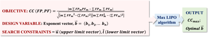
MaxLIPO problem definition
The unknown parameters in the FP expression define the search space. The output at this stage is a process/product FP expression with the best correlation (\({CC}_{max}\)) with responses, containing all candidate parameters.
-
(4)
Dimensionality reduction through recurrent feature elimination (RFE) is performed next. An ideal process or product FP shall have the minimum number of features to facilitate computational efficiency. RFE performs dimensionality reduction by eliminating the least contributing features one by one based on RFE ranking (Wang et al., 2021). A decrease in correlation coefficient is expected as features are getting eliminated, so it is vital to define a termination criterion based \({CC}_{max}\) is dropped from its maximum value. A 5% reduction is considered permissible which implies the termination of dimensionality reduction when the correlation drops below 95% \({CC}_{max}\).
-
(5)
The next step is the response prediction through the extracted process/product FP. For continuous responses, the method is relatively straightforward. An ML model is trained to predict the responses based on process/product FP as input. A stacked-ensemble ML model is used in this case for response prediction, with post-hoc explanations using XAI tools.
In ML, ensemble models use techniques to combine multiple ML predictions to enhance the accuracy than their constituent models. In comparison to its competitive ensemble techniques like bagging, and boosting, stacking has an overall better performance owing to its flexibility to combine any ML models as low-level learners and not just weak learners. The stacked ensemble can thus harness the capabilities of already well-performing models and take the overall predictive accuracy a step higher (Kim et al., 2020; Pavlyshenko, 2018). In addition, it can handle both classification and regression problems.
The ensemble technique combines the predictions of multiple base models on unseen data samples to train a meta-learner. Meta learner receives the base model predictions along with the training dataset as its input. The base and meta learners can be any capable ML model. The general architecture of a stacked ensemble model is given in Fig. 5. In this study, five base models are considered namely Ridge, Lasso, support vector regression (SVR), random forest regression (RFR), and light-gradient boost (LGB). The extreme gradient boost (XGB) algorithm is selected as the meta-learner.
Fig. 5 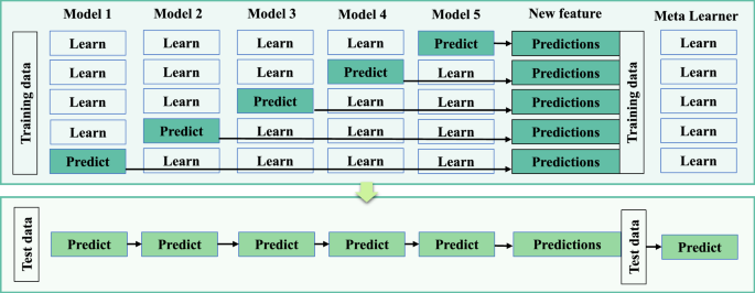
Generic stacking ensemble architecture
Prediction of categorical responses through process FP requires an additional mapping of FP values into a probabilistic scale. The overall approach for manufacturing event detection through process FP is given in Fig. 6. The steps to develop this interpretable probabilistic model are given below:
-
First, a vector of ‘n’ categorical events is transformed to a discrete integer vector (for example by assigning the values \(1, 2, 3 ... n\) for each event). With reference to Fig. 6, let the vector \(\overrightarrow{mo}=({MO}_{1},{MO}_{2},{MO}_{3}\dots ..{MO}_{n})\) represent the machining outcomes and vector \(\overrightarrow{a}=(1, 2, 3, 4, \dots n)\) represents the numeric values assigned to each of the n events. In a smart manufacturing context, such events can be defined appropriately to distinguish between a normal/healthy process state and with bottleneck/unhealthy process states like a tool failure or a process anomaly.
-
Next, the process FP is developed according to step (3), considering process parameters (machine parameters, machine controller data, and sensor signatures) as FP candidates and the categorical events (productivity, quality parameters) as output.
-
The threshold values of process FP (decision boundaries) which most appropriately differentiate one manufacturing event from another are to be defined next. The probability values are defined as a linear function of closeness to the decision boundaries. At the decision boundary, the probabilities of both events are 0.5 each. The probability of an event increases from 0.5 towards 1, as the FP value moves away from the boundary into the centroid of the event space under consideration. The event probability mapping enables online anomaly detection by monitoring just the process FP value. Stacked ensemble models are trained to predict manufacturing events based on process FP, and the rationale behind ML predictions is supported by post hoc XAI explanations.
Fig. 6 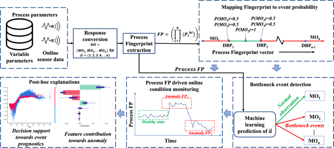
Process FP of bottleneck events
-
-
(6)
The post-hoc explanations for ML predictions are given using shapley additive explanations (SHAP) inspired by cooperative game theory. Though demonstrated for an ensemble model receiving an intrinsically explainable FP input, this approach is more relevant for explaining the decisions if the model were directly trained with a raw dataset. Both global and local interpretations are offered for the model and a single prediction respectively.
The overall logical data flow of the proposed approach is given in Fig. 7.
Fig. 7 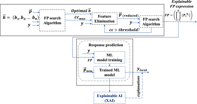
Overall dataflow of the proposed approach


Experiment details
To demonstrate the robustness of the proposed method, datasets from two processes with very different functionalities are considered. First, the framework is used to develop process and product fingerprints for a nanosecond laser ablation process to produce superhydrophobic surfaces. Secondly, the approach is validated by extracting the process FP towards building a process monitoring system for the wire EDM process. The details are as follows:
Dataset 1: Superhydrophobic surfaces through laser ablation
Due to their unique properties like low contact area and adhesion at the solid–liquid interface, superhydrophobic surfaces offer exceptional drag resistance, atmospheric corrosion resistance, dirt repellence, surface icing prevention and self-cleansing. In the first dataset, superhydrophobicity is achieved on AISI 316L stainless steel by producing micro Gaussian holes using a nanosecond laser ablation process. An open CNC-controlled ultra-precision micromachine is used for laser ablation. The experimental setup is shown in Fig. 8a. The machine has a maximum laser pulse frequency of 200 kHz, a source emission wavelength of 1064 nm and average laser output power of 20 W.

a Experimental setup of hybrid micromachining system b Surface characteristics and its effect on surface contact angle (Cai et al., 2019)
The static contact angle is measured using a drop shape analyser having a 5 μL liquid droplet volume. The surfaces are classified as superhydrophobic if the contact angle is greater than 150°. To ensure repeatability, all measurements are performed thrice and the average reading is recorded. A few selected cases demonstrating the variations in contact angle with respect to different Gaussian hole dimensions and patterns are given in Fig. 8b. Since the surface micro features have a close correlation with its water repellence, the surface geometric characteristics like arithmetic mean roughness (Sa), surface peak to valley height (Sz), surface kurtosis (Sku), surface root mean square gradient (Sdq), developed interfacial area ratio (Sdr), mean profile element width (Rsm), and largest 2D peak to valley height (Rz) are measured and recorded using a 3D surface profilometer. Experiments are conducted by varying the laser power, pitch length, and exposure time. Further details on the experiments and surface characterization can be referred to in the work done by Cai et al. (Cai et al., 2019). The process parameters are considered the potential constituent elements of a process FP expression, whereas the surface characteristic features are the potential constituent elements of a product FP expression.
Dataset 2: Wire EDM processing of inconel 718
A process monitoring dataset during wire EDM of Inconel 718 is considered to demonstrate the inclusion of online process signatures, along with machine control variables as process FP candidates. Inconel 718 is difficult to cut Nickel-based superalloy used in aerospace applications owing to its superior high-temperature performance. Conventional machining of Inconel 718 is challenging due to the material’s hardness, low thermal conductivity and chemical reactivity. Electric discharge machining is widely employed to machine the superalloys since it overcome these challenges (Markopoulos et al., 2008). In particular, wire-EDM offers a feasible solution to process such alloys due to its non-contact material removal mechanism (Abhilash & Chakradhar, 2021a, 2021b). However, pulse classification (Zhang et al., 2020) and process monitoring is essential during wire-EDM to ensure the part quality and predict process failures (Abhilash & Chakradhar, 2021c).
The experiments are conducted on a wire EDM machine having an accuracy of 1 µm on each axis. A zinc-coated brass wire of 250 µm diameter is used as the tool electrode. Dielectric fluid considered is deionized water with an electric conductivity of 20 µS/cm. An online process monitoring system comprising current and voltage sensors is also installed. Tektronix sensors and data acquisition systems have a bandwidth of 200 MHz. The operating range of the current probe is 0 to 150A and the voltage probe is 0 to 1300 V. Maximum sampling rate is 2.5 GS/s/channel, however, an ideal value of 250 MS/s/channel is selected to reduce the prediction latency.
Process parameters considered are pulse on time (TON, Mu), pulse off time (TOFF, Mu), servo voltage (SV, V), wire feed rate (WF, m/min), and the input current (Ip, A). In addition, process signatures like spark frequency (SF) and discharge energy (DE, µJ) are extracted from the real-time current and voltage sensor data. The process parameters and online signatures together constitute the process FP expression. Both continuous and categorical process responses are recorded during the machining process. Continuous responses are surface roughness (Ra, µm), cutting speed (CS, mm/min) and remaining useful life (RUL, min). One multiclass categorical response called machining outcomes has its class labels as ‘wire breakage (WB)’, ‘spark absence (SA)’ and ‘normal machining (NM)’. Among these, wire breakage and spark absence are the wire EDM failure events, which cause machining interruption, and unacceptable part quality. The dataset follows a full factorial experimental design as given in (Abhilash & Chakradhar, 2021d).
Results and discussion
Results from each computational module of the intrinsic and post-hoc XAI approaches for process/product fingerprint development are described and discussed in this section.
Interpretable representation of process/product FP for continuous responses
The proposed approach to make the process/product FP intrinsically or by design explainable is through their interpretable representations. As explained in Sect. “Interpretable fingerprint development approach”, since the form of the FP expression is determined as \(FP= \prod_{i=1}^{n}\left. ({{P}_{i}}^{bi}\right)\), the process of FP extraction boils down to finding the unknown parameters (in the current case, the exponent vector, \(\overrightarrow{b}={b}_{1}, {b}_{n},\dots \dots , {b}_{n}\)) in the expression which maximizes the product/process Fingerprint-Product Functionality (FP-PF) correlation. Due to its overall superior performance in comparison to the competitive search techniques, a MaxLIPO algorithm is selected to extract the most appropriate Process and Product FP. The details of FP extraction and performance evaluation have been demonstrated using EDM and laser ablation datasets as follows.
FP development using MaxLIPO
Dlib python library was used to perform MaxLIPO in an anaconda python distribution. Optimization constraint is defined in such a way that, each component \({(b}_{i})\) of the exponent vector \(\overrightarrow{b}\) is searched in the confined continuous space of \([- 2.5, 2.5]\). Such a selection of search constrain is from the generic understanding of mechanical processes that it is extremely unlikely to have a parameter interaction of the order greater than 2. However, for confirmation, a larger search space of \([- 5, 5]\) was also considered and the results are verified to have negligible variations in changing the search constraints. First, FP development including the full feature set is performed to extract the maximum correlation (\({CC}_{max}\)) between process/product FP and product functionality. During the developmental stage, the framework considered two objective functions: Pearson's correlation coefficient (CC) and the correlation and testing error ratio (CTER), as defined by (Kundu et al., 2022). For both objective functions, the performance of the converged solution was compared in terms of RMSE, and the following results were obtained: For the Product FP extraction of the superhydrophobic surface dataset, the RMSE improved from 0.8987 to 0.3787 (a 57.8% improvement) when CC was used as the objective function, as compared to CTER. Similarly, for the process FP, the RMSE improvement was from 0.3859 to 0.2866 (a 25.7% improvement). Consequently, CC was chosen as the preferred objective function for the framework due to its superior performance in terms of error, correlation, and computational efficiency. Details of FP extraction for both datasets are given below.
FP development for the laser ablation
For laser ablation, laser power, pitch length and exposure time have been considered as the FP constituents and contact angle as the product functionality. The MaxLIPO global optimization algorithm was used for FP extraction with the Pearson correlation coefficient as the objective function, with the exponent vector \(\overrightarrow{b}\) being the design variable. A \({CC}_{max}\) of 0.965 at \(\overrightarrow{b}=(-0.068,-0.0128, 0.063)\) was obtained as the output. The extracted process FP is given as
Next, to extract the product FP, surface geometric features Sa, Sz, Sku, Sdq, Sdr, and Rhy are considered as the constituents. The algorithm converged to provide a \({CC}_{max}\) of 0.94 at \(\overrightarrow{b}=(- 0.018, - 0.03, - 0.015, - 0.028, 0.043, - 0.092)\). Figure 9a and b show the convergence plot for process and product FP extraction respectively. The product FP is given by

Variation of fitness value (CC) with iterations during MaxLIPO search for a Process FP b Product FP
It is worth noting that the prediction of product functionality through product FP can lead to design-driven systems, where the design characteristics can be tweaked to maximize performance.
Process FP development for EDM
Both process parameters and online process signatures are considered potential candidates for process FP in the wire EDM monitoring dataset. The process parameters considered are pulse on time, pulse off time, servo voltage, wire feed rate and the input current. In-process signatures are spark frequency and discharge energy. The process FP was extracted with a \({CC}_{max}\) of 0.931 as given by the expression
Subsequently, process FPs with \({CC}_{max}\) of 0.97 and 0.87 were obtained for Ra and RUL as responses respectively. The corresponding \(\overrightarrow{b}\) for Ra and RUL are [− 0.067, 0.0319, 0.0243, − 0.040, 0.00022, − 0.0019, − 0.0036] and [0.0174, − 0.005, − 0.003, − 0.005, − 0.00047, − 0.00045, 0.0015] respectively.
Though the FPs gives the maximum correlation with functional performance, it is computationally intensive to extract and use FPs with all available parameters/surface geometric features. Finding a reduced order FP without compromising much on the correlation is often more significant with regard to computational efficiency and reduced prediction latency. In addition, dimensionality reduction can also contribute towards optimal sensor selection. Identification of a reduced order FP through Recursive Feature Elimination (RFE) keeping \({CC}_{max}\) (from the full order FP) as a reference, is discussed next.
Final FP selection through dimensionality reduction
Recursive Feature Elimination (RFE) is an ML technique for dimensionality reduction. In this approach a model is initially developed with a full feature set, having ‘n’ parameters. Then the least important feature is eliminated and the model has developed again with the reduced dataset having (n−1) parameters. This is repeated till the required number of features is eliminated or a predefined termination criterion is met. It is important to note that feature reduction methods represent a compromise between computational efficiency and the desired level of accuracy. The extent of this compromise may vary depending on the application. In this study, a 5% reduction from the maximum attainable accuracy (\({CC}_{max}\)) is considered as the threshold for accepting the reduced-order fingerprints. For manufacturing applications with stricter accuracy requirements or a greater emphasis on accuracy over computational efficiency, the threshold can be reduced to an even lower value.
RFE ranking of process parameters and surface characteristics for the laser ablation dataset is given in Table 1. Similarly, the RFE process parameter ranking for EDM is given in Table 2 considering CS, Ra, and RUL.
Reduced dimension process FP and product FP are developed by eliminating features in the order of RFE rankings discussed and listed earlier. After each feature reduction, new \(CC\) is compared with \({CC}_{max}\). Though it is expected that the \(CC\) reduces with each feature elimination, it is important to set an appropriate threshold as termination criteria to ensure that \(CC\) is still in a tolerable range. Here, a 5% reduction from \({CC}_{max}\) is considered acceptable. Thus, the set criterion is that the feature elimination gets terminated when the \(CC\) falls less than 95% of \({CC}_{max}\). The variation of \(CC\) versus the number of features considering process FP and product FP for the laser ablation process is given in Fig. 10a and b respectively.

Variation of Pearson correlation coefficient with respect to number of parameters for a process FP b product FP
Through this approach, the dimension of process FP is reduced to 2 from 3, and that of product FP is reduced from 6 to 2. \(CC\) of the reduced process and product FP are computed as 0.9595 and 0.929 respectively, which is very close to their corresponding \({CC}_{max}\) values. The variation of process FP and product FP with respect to the product functionality is shown in Fig. 11.

Variation of contact angle with respect to a process FP b product FP
The overall performance comparison of the proposed approach with the state-of-the-art in terms of \(CC\) and the number of features is given in Table 3 for the laser ablation dataset. The proposed approach clearly outperforms the existing FP development strategies based on process physics and random forest regression (RFR) in terms of \(CC\) and parameter reduction. In addition, the computational efficiency is significantly better in terms of the number of computational steps. In comparison to the exhaustive search strategy proposed in (Kundu et al., 2022), where process and product FP identification took 4913 and 531,441 computations respectively, the proposed approach converged within 2000 iterations for all cases.
Table 4 shows the details of process FP for EDM responses before and after dimensionality reduction. It is worth noting that, for all the EDM responses, the process FP dimension is reduced from 7 to 4 through dimensionality reduction. \(CC\) of the newly computed fingerprints are 0.924, 0.97 and 0.861 respectively for CS, Ra and RUL, which are greater than 95% of their corresponding \({CC}_{max}\).
Response prediction based on process FP
In the context of explainable AI, linear regression and stacked ensemble models are at opposite ends of the interpretability spectrum. Linear regression models are ‘by-design’ interpretable since it provides an equation of the form \(y=m\times FP+c\) to represent the response variable as a function of process or product FP. Though its prediction rationale is clear being a transparent or white box model, its prediction accuracy can be lesser in comparison with more advanced ML models. On the other hand, ensemble models are one of the best performing among ML algorithms since they use techniques to combine and better the prediction accuracy of multiple ML models. However, their complex computational architecture makes it one of the least interpretable ML models.
For continuous responses, both linear regression and stacked ensemble models are developed to predict the functional performance with process/product FP as inputs. For categorical responses, the response transformation and probability mapping method described in Sect. “Interpretable fingerprint development approach”—Fig. 6 is followed for FP development and subsequent response prediction.
Response prediction for laser ablation
The coefficient of determination (\({R}^{2}\)) values for the regression models to predict contact angles based on process and product FP was 0.92 and 0.86 respectively. The linear regression equations are:
It is important to note that the extraction of FPs relies on the prior selection of the power function as the FP expression (as explained in Sect. “Interpretable fingerprint development approach”, point (2) and given by Eq. (4)), and the linearity of the FP-PF relationship depends on the level of conformity of FP to the power function. Though the extracted FPs have shown significant improvement compared to existing approaches (as detailed in Table 3), there is still room for improving prediction accuracy, as FP and PF may contain other minor correlations beyond the considered power function.
The fundamental principle of ensemble learning is harnessed to capture such secondary correlations and enhance overall prediction accuracy. The stacked ensemble model combines a set of already capable models to provide better accuracy than each individual model considered. Figure 12 depicts the concept for the case of product FP. A better R2 value of 0.95 was observed using a stacked ensemble model. It can be observed from Fig. 13 that the prediction accuracy of the stacked ensemble is much closer to experimental results compared to the linear regression model. To demonstrate the superior performance of stacking, it is compared with other ML models like extreme gradient boost (XGB), random forest regression (RFR) and linear regression. The stacked ensemble clearly outperformed the other models in terms of model accuracy, as defined by \({R}^{2}\) values, the details of which are shown in Fig. 14.

Response prediction using stacked ensemble

Comparison of ensemble prediction and linear regression with experimental values for a process FP b Product FP

Performance comparison of different ML models
Response prediction for EDM
The linear regression equations for various responses are
\({R}^{2}\) values for the responses CS, Ra and RUL using linear regression are 0.83, 0.89, and 0.69 respectively. Through ensemble modelling, an improved \({R}^{2}\) of 0.93, 0.97 and 0.861 are obtained for CS, Ra, and RUL respectively.
Extending the FP development approach for bottleneck events
A novel approach is introduced to extend the concept of process FP for categorical responses. Once successfully implemented, the diagnostics and prognostics of bottleneck events can be done just by tracking/monitoring the process FP. The acceptable range of process FP for an ideal/healthy manufacturing process condition is defined in terms of the probability of manufacturing events.
As described in Sect. “Interpretable fingerprint development approach”, the idea is to transform the categorical responses into an integer space by assigning distinct numeric values to each event. This is demonstrated using the EDM dataset which has a categorical response labelled as ‘machining outcome (MO)’. The various class labels assigned for MO are spark absence (SA), normal machining (NM) and wire breakage (WB), among which NM is the ideal desirable machining state and the other two are process failures. Since these events are mutually exclusive, integers 1, 2 and 3 are assigned to SA, NM and WB respectively. The increasing order of feature importance according to RFE is TON, TOFF, WF, SV, IP, DE and SF. Based on this, the full and reduced order process FPs are given as:
The computed \({CC}_{max}\) and \(CC\) values for the original and reduced dataset are 0.88 and 0.8 respectively. The drop in \(CC\) is more drastic for MO in comparison with other responses and hence, the termination criteria were met after the first feature elimination itself. This can be due to a relatively equal contribution of all features towards the machining outcome.
Figure 15 shows the variation of process FP with respect to categorical values of machining outcomes. It can be observed that a distinct FP range can be attributed towards each machining event. Next, probability mapping is performed to relate the process FP and event probabilities. This step allows the determination of manufacturing event probabilities based on the process FP values. For this purpose, a decision space and boundary have been determined. In this case, there are two decision boundary points (since the process FP is a 1D vector) to differentiate between the three machining events. For each event, probability values are assigned based on the distance from the boundary points towards the centroid of the event space under consideration. In this case, at the decision boundary (event junction), the probability of both events will be 0.5. As the centre of the event space is being approached, the probability increases towards 1, as shown in Fig. 16.

MO probability mapping on process FP axis

a Stacked ensemble prediction of machining outcomes b after rounding off c confusion matrix
Next, to predict the MO based on process FP, a stacked ensemble model is trained with an R2 of 0.9. The details are given in Fig. 15a. Since the predicted values can have fractions, the outputs are rounded off to their nearest integer (1, 2, or 3 in this case) to determine the predicted MO as shown in Fig. 15b. The confusion matrix showing overall prediction accuracy of 95.37 is given in Fig. 15c. The proposed event probability mapping based exclusively on process FP is particularly useful for real-time systems like Digital Twins, where probabilities of failure events can be displayed in real-time through a suitable human–machine interface (HMI). This allows the operators to take informed decisions at critical junctures. For the purpose of automation, the event probability data can be communicated to the process controller for real-time feedback control to prevent potential failures.
Post-hoc explanations
Though stacking has one of the best in class prediction accuracy, the computational structure is so sophisticated that often the expert is left with no feedback on the prediction logic. Dedicated post-hoc interpretations of local predictions can add transparency to such ML models without compromising accuracy. It improves the decision-making skills of experts and stakeholders by offering multiple perspectives towards examining the model predictions. The following subsections introduce and discuss Shapley additive explanations (SHAP) from cooperative game theory to interpret a few instances of local predictions. Finally, the potential of post-hoc explanations towards a better understanding of process physics is presented and discussed.
SHAP interpretations
Figure 17 shows the overall capabilities of a SHAP tool towards the local and global explainability of a black box ML model. The global impact of each parameter towards the model predictions is expressed in terms of mean absolute shapely value. Since shapley values represent the marginal contribution of a feature towards a response, the mean absolute shapley value is proportional to the feature's importance. Based on this, laser power has the maximum contribution towards the surface contact angle, followed by a pitch and finally exposure time as shown in Fig. 18a.

SHAP post-hoc predictions

Post hoc analysis using SHAP a Global feature importance b Local feature contribution
To demonstrate the local explainability, a specific observation is randomly chosen from the laser ablation dataset having the following parameter settings: laser power = 20 W; pitch = 130 µm; exposure time = 0.4 s. For the considered settings, the ensemble model has predicted a contact angle of 140.7 O, which is a relatively higher value than the average predicted value for the overall dataset, which is 136.82°.
The shapely value-based contributions plot indicating the influence of individual features on the local prediction under consideration is given in Fig. 18b. In the considered instance, laser power has the maximum contribution towards increasing the surface contact angle from the model average by \({11.11}^{^\circ }\). On the contrary, the other two parameters, pitch and exposure time have contributed towards a decrease in the surface contact angle by \({5.47}^{^\circ }\) and \({1.76}^{^\circ }\) respectively. Such individual contributions cumulatively add up towards the final prediction, which has resulted in an overall increase of \({3.88}^{O}\) (\(11.11 - 5.47 - 1.76\)) from the average.
The partial dependence plot (PDP) is a powerful tool which shows the response variation with respect to an individual parameter. PDP for pitch and exposure time is given in Fig. 19. The thick blue curve shows the variation in response for the local instance with respect to a particular feature when the remaining settings are unchanged. On the other hand, the thick grey line represents the average change in response. Variations of other sample observations are shown in light grey lines. From the PDP of pitch given in Fig. 19a, for the considered observation, if other parameters are unchanged, a decrease in pitch increases the contact angle. The vice versa is true for exposure time, as observed in Fig. 19b. This has far greater implications in the context of the hydrophobicity of the surface. Since the surfaces whose contact angle is greater than 150° are considered superhydrophobic, the PDP facilitates the decision-making on the potential parameter revisions to produce superhydrophobic surfaces. It is worth noting that under current settings, superhydrophobicity is achievable by just reducing the pitch to a value below 110 µm, and CA can go up to ~ 160° at the limiting pitch condition. On the other hand, superhydrophobicity can also be achieved by increasing the exposure time to 0.9 s, however to a maximum of only 150°. Since XAI offers multiple perspectives on increasing the CA, the most convenient/practical route towards achieving the target can now be opted by the decision maker.

Partial dependence plot for a Pitch b Exposure time
To assess the capabilities of XAI from a process control perspective, an unhealthy EDM machining state is considered. The predicted MO is 2.6 for the selected local instance, which means it is likely to have a wire breakage failure. An MO of 2.6 indicates a 60% wire breakage possibility (since \(MO=2\) indicates NM; and \(MO=3\) indicates WB). Figure 20 shows the PDP at this instance with respect to the online process signatures, SF and DE. PDP explanations reveal that decreasing the SF will make the process condition less prone to wire breakage as it takes the MO value from 2.6 to 2. Also, It is worth noting that, decreasing SF has a steeper effect on the MO as compared to DE. In EDM, reducing SF and DE is achieved by adjusting TOFF and TON/IP respectively using the machine controller. Thus, a more appropriate process control measure would be to tune TOFF to reduce SF towards ensuring process continuity and quality compliance. XAI offers a similar range of choices and explanations at each juncture towards better high-stake decisions.

Partial dependence plot for a spark frequency b Discharge energy
In addition to supporting control-level decision-making, post hoc XAI tools have significant potential to reveal the underlying process physics of manufacturing processes. Decreasing the DE or SF towards reducing the probability of wire breakage is very much in line with EDM’s physical interpretation of the wire breakage mechanism. Wire surface deterioration accelerates and leads to breakage during high-frequency short-circuit discharges. Higher discharge energy during short circuits causes deeper craters in the wire, whereas higher frequency reduces the inter-spark distance which weakens the wire electrode’s load-carrying capability (Abhilash & Chakradhar, 2022). Such post-hoc explanations can lead to a better understanding of process physics, thus aiding the experts in complex decision-making by combining existing domain knowledge and local interpretations of black box predictions.
Explainable FP representations using symbolic regression
Based on the novel approach discussed so far, the intrinsic explainability of the process and product FP is ensured by an initial selection of explainable expressions. An alternate way to infuse intrinsic explainability into a model is through a supervised machine-learning technique called symbolic regression. The interpretable algorithm searches the space of all mathematical equations to find the best fingerprint. The expression is selected based on a hybrid termination criterion considering both prediction accuracy and model simplicity. During the expression search, binary operators considered are "*", “ + ”, “− “, “/”, and “^”. Also, unary operators like “square”, “cube”, “exp”, and “log” are considered. The mean square error is the selected loss function. The final selected process FP expression for the laser ablation dataset is given as
The R2 value of the model is 0.92, and the variation of predicted CA with experimental readings are given in Fig. 21. One of the main limitations of this approach is the higher computational load to search the entire space of mathematical equations. The computational demand increases exponentially with the increase in the number of variables. In case the number of variables is more than 10, dimensionality reduction through principal component analysis is recommended. Also, the approach is relatively less accurate than the state-of-the-art deep learning/ensemble models. In short, though capable of direct extraction of fingerprint expressions, this approach suits only smaller dimensional data. Also, the approach is suited for continuous responses and is not intended to handle categorical responses like manufacturing events. Overall, MaxLIPO-based FP search method serves better as a generic approach for fingerprint extraction since it handles higher dimensions, and categorical responses alike.

Contact angle prediction through symbolic regression
Conclusions and future work
In the smart manufacturing processes, the lack of explainability of AI-based predictions has restricted informed decision-making in high stake situations. The opaqueness of current state-of-the-art models has resulted in reduced trust in AI predictions among stakeholders and end-users. The current study aims to build a completely transparent framework for process and product FP extraction considering both intrinsic and post-hoc aspects of interpretability. The intrinsically explainable FP expression is identified through MaxLIPO global search, whose correlation is found better than the one found by symbolic regression. Through this approach, a correlation coefficient of 0.96 and 0.93 are obtained for process and product FPs with respect to contact angle (product functionality), which is significantly higher than the earlier physics-based and RFR-based approaches. Also, the approach is robust to the response types, enabling extraction of explainable process FP for machining events (categorical response) for the first time. These process FPs are utilized to predict the probability of EDM machining failures through a unique probability mapping technique. Finally, a few cases on the application of post hoc explanations towards complex-decision making is demonstrated.
The key conclusions from the study are as follows:
-
It is possible to develop a completely transparent yet better-performing FP identification approach through LIPO global optimization. The correlation is better than existing physics-based, RFR, and symbolic regression methods of FP identification.
-
Fingerprints of categorical events can be identified through a technique of response transformation and probability mapping. This in turn ensures the human comprehensibility of manufacturing events through XAI integration.
-
XAI explanations can assist the experts in complex decision-making by combining existing domain knowledge and local interpretations of black box predictions.
Future work focuses on testing the model’s generalization capability against additional manufacturing datasets. Also, the feasibility of using process FPs in real-time systems like digital twins and condition monitoring will be investigated. The approach can be further equipped with unsupervised and reinforcement learning capabilities to get rid of the training phase. An additional interesting area to explore is the usage of adaptive learning techniques to tackle concept and data drift risks, due to equipment degradation and environmental conditions, so that the accuracy of system is ensured even with changing ambient/test conditions.
Data availability
The datasets used for this study are available in the following: https://pureportal.strath.ac.uk/en/publications/product-and-process-fingerprint-for-nanosecond-pulsed-laser-ablat/datasets/. https://doi.org/10.1007/s00170-021-07974-8
References
Abhilash, P. M., & Chakradhar, D. (2021a). Machine-vision-based electrode wear analysis for closed loop wire EDM process control. Advances in Manufacturing, 10(1), 131–142. https://doi.org/10.1007/s40436-021-00373-y
Abhilash, P. M., & Chakradhar, D. (2021b). Image processing algorithm for detection, quantification and classification of microdefects in wire electric discharge machined precision finish cut surfaces. Journal of Micromanufacturing. https://doi.org/10.1177/25165984211015410
Abhilash, P. M., & Chakradhar, D. (2021c). Failure detection and control for wire EDM process using multiple sensors. CIRP Journal of Manufacturing Science and Technology, 33, 315–326. https://doi.org/10.1016/j.cirpj.2021.04.009
Abhilash, P. M., & Chakradhar, D. (2021d). Wire EDM failure prediction and process control based on sensor fusion and pulse train analysis. International Journal of Advanced Manufacturing Technology, 118(5–6), 1453–1467. https://doi.org/10.1007/s00170-021-07974-8
Abhilash, P. M., & Chakradhar, D. (2022). Performance monitoring and failure prediction system for wire electric discharge machining process through multiple sensor signals. Machining Science and Technology, 26(2), 245–275. https://doi.org/10.1080/10910344.2022.2044856
Alova, G., Trotter, P. A., & Money, A. (2021). A machine-learning approach to predicting Africa’s electricity mix based on planned power plants and their chances of success. Nature Energy, 6(2), 158–166. https://doi.org/10.1038/s41560-020-00755-9
Angelov, P. P., Soares, E. A., Jiang, R., Arnold, N. I., & Atkinson, P. M. (2021). Explainable artificial intelligence: An analytical review. Wiley Interdisciplinary Reviews: Data Mining and Knowledge Discovery, 11(5), 1–13. https://doi.org/10.1002/widm.1424
Bai, Y., Sun, Z., Zeng, B., Long, J., Li, L., de Oliveira, J. V., & Li, C. (2019). A comparison of dimension reduction techniques for support vector machine modeling of multi-parameter manufacturing quality prediction. Journal of Intelligent Manufacturing, 30(5), 2245–2256. https://doi.org/10.1007/s10845-017-1388-1
Barredo Arrieta, A., Díaz-Rodríguez, N., Del Ser, J., Bennetot, A., Tabik, S., Barbado, A., et al. (2020). Explainable Artificial Intelligence (XAI): Concepts, taxonomies, opportunities and challenges toward responsible AI. Information Fusion, 58, 82–115. https://doi.org/10.1016/j.inffus.2019.12.012
Baruffi, F., Calaon, M., & Tosello, G. (2018). Micro-injection moulding in-line quality assurance based on product and process fingerprints. Micromachines. https://doi.org/10.3390/mi9060293
Bellotti, M., Qian, J., & Reynaerts, D. (2019). Process fingerprint in micro-EDM drilling. Micromachines. https://doi.org/10.3390/mi10040240
Brito, L. C., Susto, G. A., Brito, J. N., & Duarte, M. A. V. (2022). An explainable artificial intelligence approach for unsupervised fault detection and diagnosis in rotating machinery. Mechanical Systems and Signal Processing, 163, 108105. https://doi.org/10.1016/j.ymssp.2021.108105
Cai, Y., Luo, X., Liu, Z., Qin, Y., Chang, W., & Sun, Y. (2019). Product and process fingerprint for nanosecond pulsed laser ablated superhydrophobic surface. Micromachines. https://doi.org/10.3390/mi10030177
Carletti, M., Masiero, C., Beghi, A., & Susto, G. A. (2019). Explainable machine learning in industry 40: Evaluating feature importance in anomaly detection to enable root cause analysis. Conference Proceedings - IEEE International Conference on Systems, Man and Cybernetics. https://doi.org/10.1109/SMC.2019.8913901
Chiu, M. C., Chiang, Y. H., & Chiu, J. E. (2023). Developing an explainable hybrid deep learning model in digital transformation: An empirical study. Journal of Intelligent Manufacturing, 3(123), 1–18. https://doi.org/10.1007/S10845-023-02127-Y/TABLES/6
de Bruijn, H., Warnier, M., & Janssen, M. (2022). The perils and pitfalls of explainable AI: Strategies for explaining algorithmic decision-making. Government Information Quarterly. https://doi.org/10.1016/J.GIQ.2021.101666
Farbiz, F., Habibullah, M. S., Hamadicharef, B., Maszczyk, T., & Aggarwal, S. (2022). Knowledge-embedded machine learning and its applications in smart manufacturing. Journal of Intelligent Manufacturing. https://doi.org/10.1007/s10845-022-01973-6
Ghahramani, M., Qiao, Y., Zhou, M. C., Hagan, A. O., & Sweeney, J. (2020). AI-based modeling and data-driven evaluation for smart manufacturing processes. IEEE/CAA Journal of Automatica Sinica, 7(4), 1026–1037. https://doi.org/10.1109/JAS.2020.1003114
Hoffmann, L., Fortmeier, I., & Elster, C. (2021). Uncertainty quantification by ensemble learning for computational optical form measurements. Machine Learning: Science and Technology PAPER, 2, 035030.
Kim, M., Lee, M., An, M., & Lee, H. (2020). Effective automatic defect classification process based on CNN with stacking ensemble model for TFT-LCD panel. Journal of Intelligent Manufacturing, 31(5), 1165–1174. https://doi.org/10.1007/S10845-019-01502-Y/TABLES/6
Kitano, H. (2021). Nobel Turing Challenge: creating the engine for scientific discovery. Npj Systems Biology and Applications. https://doi.org/10.1038/s41540-021-00189-3
Klink, A. (2016). Process signatures of EDM and ECM processes – Overview from Part functionality and surface modification point of view. Procedia CIRP, 42, 240–245. https://doi.org/10.1016/J.PROCIR.2016.02.279
Krenn, M., Pollice, R., Guo, S. Y., Aldeghi, M., Cervera-Lierta, A., Friederich, P., et al. (2022). On scientific understanding with artificial intelligence. Nature Reviews Physics, 4(12), 761–769. https://doi.org/10.1038/s42254-022-00518-3
Kundu, P., Luo, X., Qin, Y., Cai, Y., & Liu, Z. (2022). A machine learning-based framework for automatic identification of process and product fingerprints for smart manufacturing systems. Journal of Manufacturing Processes, 73, 128–138. https://doi.org/10.1016/j.jmapro.2021.10.060
Kuriakose, S., Parenti, P., & Annoni, M. (2020). Micro extrusion of high aspect ratio bi-lumen tubes using 17–4PH stainless steel feedstock. Journal of Manufacturing Processes, 58, 443–457. https://doi.org/10.1016/J.JMAPRO.2020.07.059
Lee, C. Y., & Chien, C. F. (2022). Pitfalls and protocols of data science in manufacturing practice. Journal of Intelligent Manufacturing, 33(5), 1189–1207. https://doi.org/10.1007/s10845-020-01711-w
Lee, M., Jeon, J., & Lee, H. (2022). Explainable AI for domain experts: A post Hoc analysis of deep learning for defect classification of TFT–LCD panels. Journal of Intelligent Manufacturing, 33(6), 1747–1759. https://doi.org/10.1007/S10845-021-01758-3/FIGURES/17
Lundberg, S. M., & Lee, S. I. (2017). A unified approach to interpreting model predictions. Advances in Neural Information Processing Systems, 30, 4766–4775.
Malherbe, C., & Vayatis, N. (2017). Global optimization of Lipschitz functions. In Proceedings of the 34th International Conference on Machine Learning (pp. 3592–3601).
Markopoulos, A. P., Manolakos, D. E., & Vaxevanidis, N. M. (2008). Artificial neural network models for the prediction of surface roughness in electrical discharge machining. Journal of Intelligent Manufacturing, 19(3), 283–292. https://doi.org/10.1007/s10845-008-0081-9
Meister, S., Wermes, M., Stüve, J., & Groves, R. M. (2021). Investigations on explainable artificial intelligence methods for the deep learning classification of fibre layup defect in the automated composite manufacturing. Composites Part b: Engineering, 224, 109160. https://doi.org/10.1016/j.compositesb.2021.109160
Nti, I. K., Adekoya, A. F., Weyori, B. A., & Nyarko-Boateng, O. (2022). Applications of artificial intelligence in engineering and manufacturing: A systematic review. Journal of Intelligent Manufacturing. https://doi.org/10.1007/s10845-021-01771-6
Obregon, J., & Jung, J. Y. (2022). Rule-based visualization of faulty process conditions in the die-casting manufacturing. Journal of Intelligent Manufacturing. https://doi.org/10.1007/S10845-022-02057-1/TABLES/8
Obregon, J., Hong, J., & Jung, J. Y. (2021). Rule-based explanations based on ensemble machine learning for detecting sink mark defects in the injection moulding process. Journal of Manufacturing Systems, 60, 392–405. https://doi.org/10.1016/j.jmsy.2021.07.001
Park, H., Ali, A., Mall, R., Liu, T., & Barnard, A. S. (2021). Fast derivation of Shapley based feature importances through feature extraction methods for nanoinformatics. Machine Learning: Science and Technology, 2(3), 035034. https://doi.org/10.1088/2632-2153/AC0167
Pavlyshenko, B. (2018). Using Stacking Approaches for Machine Learning Models. In Proceedings of the 2018 IEEE 2nd International Conference on Data Stream Mining and Processing, DSMP 2018 (pp. 255–258). IEEE. https://doi.org/10.1109/DSMP.2018.8478522
Qiao, H., Wang, T., & Wang, P. (2020). A tool wear monitoring and prediction system based on multiscale deep learning models and fog computing. International Journal of Advanced Manufacturing Technology, 108(7–8), 2367–2384. https://doi.org/10.1007/s00170-020-05548-8
Rostami, H., Blue, J., & Yugma, C. (2017). Equipment condition diagnosis and fault fingerprint extraction in semiconductor manufacturing. Proceedings - 2016 15th IEEE International Conference on Machine Learning and Applications, ICMLA 2016, (pp. 534–539). https://doi.org/10.1109/ICMLA.2016.90
Rudin, C. (2019). Stop explaining black box machine learning models for high stakes decisions and use interpretable models instead. Nature Machine Intelligence, 1(5), 206–215. https://doi.org/10.1038/s42256-019-0048-x
Scime, L., & Beuth, J. (2019). Using machine learning to identify in-situ melt pool signatures indicative of flaw formation in a laser powder bed fusion additive manufacturing process. Additive Manufacturing, 25, 151–165. https://doi.org/10.1016/j.addma.2018.11.010
Sofianidis, G., Rožanec, J. M., Mladenićand, D., & Kyriazis, D. (2021). A review of explainable artificial intelligence in manufacturing. Trusted Artificial Intelligence in Manufacturing: A Review of the Emerging Wave of Ethical and Human Centric AI Technologies for Smart Production. https://doi.org/10.1561/9781680838770.ch5
Suarez, A., Aldalur, E., Veiga, F., & Artaza, T. (2021). Wire arc additive manufacturing of an aeronautic fitting with different metal alloys: From the design to the part. Journal of Manufacturing Processes, 64, 188–197. https://doi.org/10.1016/j.jmapro.2021.01.012
Tiensuu, H., Tamminen, S., Puukko, E., & Röning, J. (2021). Evidence-based and explainable smart decision support for quality improvement in stainless steel manufacturing. Applied Sciences, 11(22), 10897. https://doi.org/10.3390/app112210897
Vahdat, M. T., Agrawal, K. V., & Pizzi, G. (2022). Machine-learning accelerated identification of exfoliable two-dimensional materials. Machine Learning: Science and Technology, 3(4), 045014. https://doi.org/10.1088/2632-2153/AC9BCA
Vollert, S., Atzmueller, M., & Theissler, A. (2021). Interpretable Machine Learning: A brief survey from the predictive maintenance perspective. IEEE International Conference on Emerging Technologies and Factory Automation, ETFA, 2021-Septe. https://doi.org/10.1109/ETFA45728.2021.9613467
Wang, Y., Cui, W., Vuong, N. K., Chen, Z., Zhou, Y., & Wu, M. (2021). Feature selection and domain adaptation for cross-machine product quality prediction. Journal of Intelligent Manufacturing. https://doi.org/10.1007/S10845-021-01875-Z/FIGURES/5
Yan, H. S., An, Y. W., & Shi, W. W. (2010). A new bottleneck detecting approach to productivity improvement of knowledgeable manufacturing system. Journal of Intelligent Manufacturing, 21(6), 665–680. https://doi.org/10.1007/s10845-009-0244-3
Zanjani, M. Y., Hackert-Oschätzchen, M., Martin, A., Meichsner, G., Edelmann, J., & Schubert, A. (2019). Process control in jet electrochemical machining of stainless steel through inline metrology of current density. Micromachines. https://doi.org/10.3390/mi10040261
Zhang, X., Liu, Y., Wu, X., & Niu, Z. (2020). Intelligent pulse analysis of high-speed electrical discharge machining using different RNNs. Journal of Intelligent Manufacturing, 31(4), 937–951. https://doi.org/10.1007/s10845-019-01487-8
Acknowledgements
The authors gratefully acknowledge the financial support from the UK Engineering and Physical Sciences Research Council (EPSRC, EP/ T024844/1, EP/V055208/1, W004860/1).
Funding
Engineering and Physical Sciences Research Council, EP/T024844/1, Xichun Luo
Author information
Authors and Affiliations
Corresponding author
Ethics declarations
Conflict of interest
The authors declare that they have no known competing financial interests or personal relationships that could have appeared to influence the work reported in this paper.
Additional information
Publisher's Note
Springer Nature remains neutral with regard to jurisdictional claims in published maps and institutional affiliations.
Rights and permissions
Open Access This article is licensed under a Creative Commons Attribution 4.0 International License, which permits use, sharing, adaptation, distribution and reproduction in any medium or format, as long as you give appropriate credit to the original author(s) and the source, provide a link to the Creative Commons licence, and indicate if changes were made. The images or other third party material in this article are included in the article's Creative Commons licence, unless indicated otherwise in a credit line to the material. If material is not included in the article's Creative Commons licence and your intended use is not permitted by statutory regulation or exceeds the permitted use, you will need to obtain permission directly from the copyright holder. To view a copy of this licence, visit http://creativecommons.org/licenses/by/4.0/.
About this article

Cite this article
Puthanveettil Madathil, A., Luo, X., Liu, Q. et al. Intrinsic and post-hoc XAI approaches for fingerprint identification and response prediction in smart manufacturing processes. J Intell Manuf (2024). https://doi.org/10.1007/s10845-023-02266-2
Received:
Accepted:
Published:
DOI: https://doi.org/10.1007/s10845-023-02266-2