
Abstract
We discuss the tension between the possible existence of Painlevé–Gullstrand coordinate systems versus the explicit geometrical features of the Kerr spacetime; a subject of interest to Professor Thanu Padmanabhan in the weeks immediately preceding his unexpected death. We shall carefully distinguish strong and weak Painlevé–Gullstrand coordinate systems, and conformal variants thereof, cataloguing what we know can and cannot be done—sometimes we can make explicit global statements, sometimes we must resort to implicit local statements. For the Kerr spacetime the best that seems to be achievable is to set the lapse function to unity and represent the spatial slices with a 3-metric in factorized unimodular form; this arises from considering the Doran version of Kerr spacetime in Cartesian coordinates. We finish by exploring the (limited) extent to which this construction might possibly lead to implementing an “analogue spacetime” model suitable for laboratory simulations of the Kerr spacetime.
1 Introduction
In late August 2021, just a few weeks before his unexpected passing, Professor Thanu Padmanabhan expressed an interest in the interplay between Painlevé–Gullstrand coordinates [1,2,3], or more generally spatially-flat coordinate systems, and the Kerr spacetime geometry [4,5,6,7,8,9,10]. Extracted (with very minor edits) from an e-mail from TP to MV dated 25 August 2021:
Many spacetimes admit a 1+3 foliation such that the spatial sections are flat. (This is, of course what happens in PG coordinates). Given the metric in an arbitrary coordinate system is there a geometrical condition (necessary/sufficient) for such a foliation to exist?
Since we still have shift and lapse there are 4 dof; and arbitrary metric has 6 dof. So we have “only” lost 2 dof.... So I would expect wide class of spacetimes to allow this.
Once you are in such a foliation all the curvature scalars of 3 space vanishes. Writing them in terms of 4-d curvature plus \(K_{ab}\) etc one can write down some necessary conditions but which seem difficult to reduce to simple geometrical features.
Any literature reference will also be useful.
MV responded on 27 August 2021, and that response, (now greatly expanded and elaborated), is the ultimate basis for the extensive discussion below. The fundamental reason these considerations are so interesting is the tension between the relative tractability of those spacetime metrics that can be expressed in Painlevé–Gullstrand coordinates [11, 12], and the overwhelming pedagogical [13,14,15,16,17,18,19,20,21,22], theoretical [23,24,25], and astrophysical [26,27,28,29,30,31] importance of the Kerr spacetime.
2 Preliminaries
We shall start by distinguishing strong and weak forms of the Painlevé–Gullstrand coordinate systems [1,2,3], and then—by extension—conformal versions of the (strong/weak) Painlevé–Gullstrand coordinate systems.
2.1 Strong Painlevé–Gullstrand coordinates
We shall say that a coordinate system is of strong Painlevé–Gullstrand form if the spacetime line element can be written as
That is, the metric can be cast in the form
Equivalently, for the inverse metric
Here \(v^i(t,\textbf{x})= \delta ^{ij} \, v_j(t,\textbf{x})\). In the language of the ADM formalism [32, 33] the lapse function, typically denoted \(N(t,\textbf{x})\), is unity and the spatial 3-slices are flat. For this class of metrics all nontrivial aspects of the spacetime geometry have been shoe-horned into the shift vector \(N_i(t,\textbf{x}) = g_{ti}(t,\textbf{x}) = - v_i(t,\textbf{x})\). The relative minus sign appearing herein, \(N_i = - v_i\), is merely formal—a historical accident ultimately due to differing conventions between the ADM and analogue spacetime communities. Note however, that there is an additional choice of sign implicit in the choice between “ingoing” and “outgoing” Painlevé–Gullstrand coordinates; a distinction equivalent to reversing the sign of the time coordinate.Footnote 1
Algebraically this strong Painlevé–Gullstrand form can be achieved if and only if there exist two distinct 4-orthogonal 4-vectors—a covariant vector \(T_a=(-1;0,0,0)\) and a contravariant vector \(F^a=(0; v^i)\), satisfying \(T_a F^a=0\), such that the metric factorizes in the specific form:
Here as usual \(\eta _{ab} = {\textrm{diag}}(-1,1,1,1)\). Expanding, one has
Thence, since \((\delta _a{}^c - T_a F^c) (\delta _c{}^b + T_c F^b) = \delta ^a{}_b\), for the inverse metric we have:
Expanding
Note that we must then have \(g^{ab} T_b = (1;v^i)\), whereas \(g_{ab} F^b = (\{\delta _{jk} v^j v^k\}; v_i)\). Thence \(g^{ab} T_a T_b = -1 = \eta ^{ab} T_a T_b\), while \(g_{ab} F^a F^b = \{\delta _{jk} v^j v^k\} = \eta _{ab} F^a F^b\). Thus \(T_a\) is a timelike unit co-vector with respect to both \(g^{ab}\) and \(\eta ^{ab}\), while \(F^a\) is a spacelike vector with respect to both \(g_{ab}\) and \(\eta _{ab}\).
Note the extremely strong constraint on the co-vector \(T_a\). One has \(T_a= (-1,0,0,0)\) which implies \(T_{[a,b]}=0\); so in the language of differential forms one has \(T = - {\textrm{d}}t\) and \({\textrm{d}}T =0\). It is this \({\textrm{d}}T=0\) constraint that will ultimately prove problematic for Kerr spacetime.
Known examples of such strong Painlevé–Gullstrand behaviour are:
-
All of Schwarzschild spacetime; \(r>0\). (See for example [11, 12] and [34]. For Schwarzschild spacetime one has \(\textbf{v} = \mp \sqrt{2m/r}\; {\hat{r}}\) for black holes/white holes respectively.
-
Most of Reissner–Nordström spacetime; the region \(r\ge Q^2/(2m)\). For Reissner–Nordström spacetime one has \(\textbf{v} = \mp \sqrt{2m/r-Q^2/r^2}\; {\hat{r}}\) for black holes/white holes respectively. This becomes imaginary for \(r<Q^2/(2m)\). Since (for the usual black hole situation \(m>|Q|\)) the region \(r\le Q^2/(2m)\) lies below the inner (Cauchy) horizon, this deep-core breakdown of the strong Painlevé–Gullstrand coordinates is not particularly worrisome. (See for example [12].) Even for an extremal Reissner–Nordström black hole, \(m=|Q|\), the horizon is at \(r_H=m\) while the breakdown of Painlevé–Gullstrand coordinates occurs at m/2, well below the (extremal) horizon. Finally for the case of naked singularities, (when \(m<|Q|\)), the breakdown of Painlevé–Gullstrand coordinates at \(r\le Q^2/(2m)\) is itself “naked” and in principle visible from asymptotic infinity.
-
Spatially flat \(k=0\) FLRW cosmologies, and Kottler (Schwarzschild-de Sitter) spacetimes [35, 36].
-
The Lense–Thirring (slow-rotation Kerr) spacetime [37, 38] also has a strong Painlevé–Gullstrand implementation [39,40,41,42].
-
This also works (essentially by definition) for the generic Natario class of warp-drive spacetimes (including the Alcubierre, zero-expansion, and zero-vorticity warp drives) [43, 44].
-
This also works (essentially by definition) for the tractor/pressor/stressor beam spacetimes [45, 46].
Known examples of spacetimes that are incompatible with such strong Painlevé–Gullstrand behaviour are:
-
Kerr (and the Kerr–Newman) spacetimes. The non-existence proof is quite tricky and indirect, using asymptotic peeling properties of the 3-dimensional Cotton–York tensor [47, 48]. The spatial 3-slices cannot even be made conformally flat, let alone Riemann flat. There is also evidence that the 3-metric characterizing the spatial slices cannot even be diagonalized without adverse effects on other aspects of the Kerr geometry [49].
-
The van den Broeck warp drive [50, 51], a warp drive variant wherein the spatial 3-slices are allowed to be conformally flat instead of being Riemann flat.
2.2 Weak Painlevé–Gullstrand coordinates
We shall say that a coordinate system is of weak Painlevé–Gullstrand form if the spacetime line element can be written as
That is, the metric can be cast in the form
Equivalently, for the inverse metric
In the language of the ADM formalism [32, 33] the lapse function \(N(t,\textbf{x})\) is now allowed to be non-trivial, while the spatial 3-slices are still flat.
Finding a factorized form of the metric is now a little trickier — by considering the sub-case \(v_i(x)\rightarrow 0\) it becomes clear that it is useful to consider the matrix \((\eta _N)_{ab} = {\textrm{diag}}\{-N^2;1,1,1\}\). Then algebraically weak Painlevé–Gullstrand behaviour can be achieved if and only if there exist two 4-vectors \(T_a=(-N;0,0,0)\) and \(F^a=(0; v^i/N)\) such that \(F^a T_a =0\) and the metric factorizes in the following manner:
Expanding
For the inverse metric we now have
Expanding
Here we define \((\eta _N)^{cd}= {\textrm{diag}}\{-N^{-2};1,1,1\}\).
Thence \(g^{ab} T_b = (1,v^i)/N\), and similarly \(g_{ab} F^b = (\{\delta _{jk} v^j v^k\}; v_i)/N\). This implies \(g^{ab} T_a T_b = -1 = (\eta _N)^{ab} T_a T_b\), while \(g_{ab} F^a F^b = \{\delta _{jk} v^j v^k\}/N^2 = (\eta _N)_{ab} F^a F^b\), and \(F^aT_a=0\). Thus \(T_a\) is a timelike unit vector with respect to both \(g^{ab}\) and \((\eta _N)^{ab}\), while \(F^a\) is a spacelike vector with respect to both \(g_{ab}\) and \((\eta _N)_{ab}\), and these two 4-vectors are 4-orthogonal.
Note the extremely strong constraint on the co-vector \(T_a\): We have \(T_a= (-N,0,0,0)\) which implies \(T_{[a,b]}=N_{[,a} T_{b]}/N\) whence \(T_{[a,b} T_{c]}=0\); in the language of differential forms \(T = - N {\textrm{d}}t\) and \(T\wedge {\textrm{d}}T =0\). It is this \(T\wedge {\textrm{d}}T=0\) constraint that will ultimately prove problematic for Kerr spacetime.
Known examples of such weak Painlevé–Gullstrand behaviour include:
-
All strong Painlevé–Gullstrand metrics are special cases of the weak form.
-
Analogue spacetimes in the eikonal (ray optics, ray acoustics) limit [52,53,54,55,56,57,58,59,60]; where the lapse function is to be interpreted as the signal propagation speed, \(N(t,\textbf{x})\rightarrow c_s(t,\textbf{x})\), and the shift vector is to be interpreted as minus the 3-velocity of the medium, \(N_i(t,\textbf{x}) = g_{ti}(t,\textbf{x})= - v_i (t,\textbf{x})\).
-
Spherical symmetry: Most spherically symmetric spacetimes, even if time-dependent, can at least locally be put in weak Painlevé–Gullstrand form [61]. The major obstructions to putting spherically symmetric spacetimes into weak Painlevé–Gullstrand form are the possible existence of wormhole throats, (where the area coordinate r would fail to be monotone), or situations where the Misner–Sharp quasi-local mass m(r, t) is negative (where the shift vector would become imaginary) [12]. In terms of the Misner–Sharp quasi-local mass one can write the spherically symmetric weak-Painlevé–Gullstrand metric in the form
$$\begin{aligned} g_{ab} = \left[ \begin{array}{c|c} -N(r,t)^2\{1-2m(r,t)/r \} &{} \mp N(r,t) \sqrt{2m(r,t)/r} \; {\hat{r}}_i\\ \hline \mp N(t) \sqrt{2m(r,t)/r} \; {\hat{r}}_i &{} \delta _{ij} \end{array} \right] . \end{aligned}$$(2.16)The inverse (contravariant) metric is
$$\begin{aligned} g^{ab} = \left[ \begin{array}{c|c} -N(r,t)^{-2} &{} \mp N(r,t)^{-1} \sqrt{2m(r,t)/r} \; {\hat{r}}_i\\ \hline \mp N(t)^{-1} \sqrt{2m(r,t)/r} \; {\hat{r}}_i &{} \delta ^{ij} - \frac{2m(r,t)}{r} \; {\hat{r}}^i \; {\hat{r}}^j \end{array} \right] . \end{aligned}$$(2.17)This explicit form of the metric makes manifest the requirement for positive Misner–Sharp quasi-local mass. In particular, any spherically symmetric spacetime violating the positive mass theorem cannot be put into weak-Painlevé–Gullstrand form. Conversely if the spacetime can be put into weak-Painlevé–Gullstrand form in the asymptotic region, then the spacetime must have positive ADM mass. Finally note that even when one can prove the local existence of these weak-Painlevé–Gullstrand coordinates, actually finding the relevant coordinate transformation might in practice be prohibitively difficult [35, 61].
Known examples that are incompatible with such weak Painlevé–Gullstrand behaviour are:
-
Kerr (and Kerr–Newman) spacetimes. (As for the strong Painlevé–Gullstrand form, the behaviour for the weak Painlevé–Gullstrand form is no better.)
-
The van den Broeck warp drive [50, 51]. (As for the strong Painlevé–Gullstrand form, the behaviour for the weak Painlevé–Gullstrand form is no better.)
2.3 Conformal (strong/weak) Painlevé–Gullstrand coordinates
We shall say that a coordinate system is of conformal Painlevé–Gullstrand form if the spacetime line element is conformal to (either strong or weak versions of) the Painlevé–Gullstrand line element. Either
or
The existence of these conformal Painlevé–Gullstrand line elements is a relatively weak constraint, though still enough to preclude the Kerr or Kerr–Newman spacetimes. The factorization properties we saw for strong or weak Painlevé–Gullstrand situations continue to hold with only a minimal amount of conformal rescaling.
Known examples of this conformal Painlevé–Gullstrand behaviour include:
-
The McVittie spacetime can be put into conformal weak Painlevé–Gullstrand form [35].
-
The van den Broeck warp drive [50, 51] corresponds to the special case of setting \(\Omega (t,\textbf{x})N(t,\textbf{x})\rightarrow 1\) in the conformal weak Painlevé–Gullstrand line element. That is
$$\begin{aligned} {\textrm{d}}s^2 = - {\textrm{d}}t^2 + \Omega ^2(t,\textbf{x}) \Big |{\textrm{d}}\textbf{x} - \textbf{v}(t,\textbf{x}) \; {\textrm{d}}t\Big |^2. \end{aligned}$$(2.20) -
Analogue spacetimes in the wave propagation limit, (physical optics, physical acoustics) [52,53,54,55,56,57,58,59,60] are often of this form. Here the lapse function is to be interpreted as the wave propagation speed, \(N(t,\textbf{x})\rightarrow c_s(t,\textbf{x})\), while the shift vector is to be interpreted as being proportional to minus the (typically non-relativistic) 3-velocity of the medium, \(N_i(t,\textbf{x}) = g_{ti}(t,\textbf{x})= - \Omega (t,\textbf{x}) \, v_i (t,\textbf{x})\). The presence of the overall conformal factor \(\Omega (t,\textbf{x})\) has to do with the details of deriving the relevant wave equation (d’Alembertian), and is typically some function of the background density and pressure [52, 59].
Known examples that are incompatible with such behaviour are:
-
Kerr (and Kerr–Newman) spacetimes. (As for the strong and weak Painlevé–Gullstrand forms, the behaviour for the conformal Painlevé–Gullstrand form is no better.)
2.4 Summary
In view of the comments above, we shall now put some effort into seeing just how close we can get to putting the Kerr spacetime into (strong/weak/conformal) Painlevé–Gullstrand form. It is quite remarkable just how many physically interesting spactimes can be recast in (strong/weak/conformal) Painlevé–Gullstrand form, and just how stubborn the astrophysically important Kerr spacetime is in simply refusing to be recast in this form.
3 The river model of Kerr spacetime
To develop our discussion we shall adapt the so-called “river model” of Kerr spacetime [62], which is based on the Doran coordinate system [63]. See the discussion in references [8, 9], and more recently [64]. We shall soon see that (for the Kerr spacetime) the “fluid” in the “river” is not a perfect fluid.
3.1 General framework
Appealing to the “river model” [62], we aim to establish the plausibility of generically writing the spacetime metric in the somewhat messier (non Painlevé–Gullstrand) form:
Here \(x=(t,\textbf{x})\) and the two 3-vectors \(\textbf{u}(x)\) and \(\textbf{u}(x)\) are perpendicular. We see that for \(\Omega (x)\rightarrow 1\) and \(\textbf{u}(x)\rightarrow 0\) this is simply a standard (strong) Painlevé–Gullstrand metric, and (as we have seen above) this line element is sufficient to describe very many but not all physically interesting spacetimes.
Even for \(\Omega (x)\ne 1\) and \(\textbf{u}(x)\rightarrow 0\) this is still of conformal (strong) Painlevé–Gullstrand form. But, in view of the analysis by Valiente-Kroon [47, 48], setting \(\textbf{u}(x)\rightarrow 0\) is not sufficient for describing either the Kerr or Kerr–Newman spacetimes.
On the other hand once we allow \(\textbf{u}(x)\ne 0\) (even with \(\Omega (x)\equiv 1\)) this is general enough to describe the Kerr geometry. See (for example) references [62, 63]. Once we additionally allow \(\Omega (x)\ne 1\) then, at least from the point of view of counting degrees of freedom, this this is general enough to describe describe an arbitrary spacetime.
To see how the counting argument works: Note that in four dimensions the metric \(g_{ab}\) has ten algebraically independent components. Apply four coordinate conditions on your coordinate chart. This leaves six “physical” degrees of freedom. (Off-shell, before imposing the Einstein equations.) The ansatz has the required six degrees of freedom, three in the vector \(\textbf{v}(x)\), two more in the orthogonal vector \(\textbf{u}(x)\), and one remaining degree of freedom in in the conformal factor \(\Omega (x)\).
Let us now rewrite the assumed line element (3.1) as:
That is
Here we have introduced two 4-orthogonal 4-vectors
Expanding, we recover (3.1) as asserted. The utility of introducing the two 4-vectors \(\alpha _m\) and \(\beta ^m \) is that it allows for a very simple specification of a suitable orthonormal co-tetrad and tetrad. (That the existence of a globally defined co-tetrad, and its associated globally defined tetrad, is physically important is discussed in reference [65].) Note that these 4-vectors \(\alpha _m\) and \(\beta ^m \) are very close in spirit to the 4-vectors \(T_a\) and \(F^a\) we introduced when discussing the strong and weak Painlevé–Gullstrand forms of the metric. The key difference is that now
with the overall sign flip just being a physically unimportant historical accident. The non-trivial part of this new construction is the introduction of the 3-vector \(u_i(t,\textbf{x})\).
Using these definitions let us now write the Kerr metric as
Then co-tetrad and tetrad can be taken to be
Thence
It is the 4-orthogonality of \(\alpha \) and \(\beta \) that keeps the matrix inversion relating tetrad and co-tetrad simple. The inverse metric is
To be fully explicit
and
3.2 Issues specific to Kerr spacetime
Let us now deal with some issues of specific relevance to the Kerr spacetime, which we shall conveniently write here in its Doran form
Here the quantities \(\beta \), R, \(\rho \), and r, are ultimately functions of the coordinates \(\{x,y,z\}\), and the parameters \(\{m,a\}\). Explicitly
and
while
Finally, note that the Doran time and azimuthal angle used in the above metric are related to those of the standard Boyer–Lindquist coordinates \((t_{BL},\phi _{BL})\) via the simple relations
3.2.1 Flow and twist vectors
In their “river model of black holes” paper, (their equation (30) and thereafter), Hamilton and Lisle [62] describe how to recast the above line element Eq. (3.12) into the form
with
Thence
That is, for the Kerr spacetime they can get away with setting \(\Omega \rightarrow 1\). Explicitly, (in the Cartesian form of the Doran coordinates that they adopt), they report
and
Here \(v^i\) is what they call the “flow” vector and \(u_i\) is what they call the “twist” vector. (The relation of this twist vector to vorticity being not entirely clear—more on this point below.) Note \(v^i u_i=0\), in concordance with our general discussion above.
Note that the twist vector \(u_i\) is independent of the mass parameter m, it just depends on the spin parameter a. Moreover, the only place that the mass parameter m shows up is in the quantity \(\beta \), which is a pre-factor in the flow vector \(u^i\). For the 4-vectors \(\alpha _m\) and \(\beta ^m \), and so implicitly the “twist” and the “flow”, for the Kerr spacetime one has
and
To be fully explicit, it is sometimes useful to observe:
while
and
Then for the Kerr solution explicit computation yields \(\nabla \cdot \textbf{u}=0\), so the twist vector is at least solenoidal (divergence free). Unfortunately the “vorticity” \(\nabla \times \textbf{u}\ne 0\) is both non-zero and rather messy. Similarly the helicity \(\textbf{u} \cdot (\nabla \times \textbf{u})\ne 0\) and Lamb vector \(\textbf{u} \times (\nabla \times \textbf{u})\ne 0\) are both non-zero and quite messy. In view of the axial symmetry and the solenoidal condition on the twist, there must be a vector potential for the twist of the form
with \(\Psi (x,y,z,a)\) a somewhat messy axisymmetric function of its variables.
Similarly one can calculate both \(\nabla \cdot \textbf{v}\ne 0\) and \(\nabla \times \textbf{v}\ne 0\) for the flow vector \(\textbf{v}\), though now both of these quantities are nonzero. Finally, the extension to Kerr–Newman spacetime is straightforward—in the metric/line-element one simply replaces \(m \rightarrow m - {1\over 2} Q^2/r\) in the function \(\beta \), no other changes are required.
In summary, the ansatz
is sufficiently general to include the Kerr and Kerr–Newman spacetimes. The spatial slices are however emphatically not flat, so they are not compatible with any of the usual formulations of Painlevé–Gullstrand coordinates, a point we shall expand on more fully below.
3.2.2 Geometry of 3-space
Let us now focus on the geometry of the spatial slices in Kerr spacetime. Temporarily returning to our general ansatz, strip out the conformal factor (\(\Omega \rightarrow 1\)) and consider the simplified ansatz:
Expand:
Defining \(v_i = \delta _{ij} v^j\), one can read off the 3-metric:
Note that only when the twist vector vanishes \(\textbf{u} \rightarrow 0\) does one regain flat spatial slices, while still keeping a nontrivial spacetime due to a nonzero flow.Footnote 2 Note further that, because of the 3-orthogonality of the twist vector u and flow vector v, we have \(\det (\delta _{ij} - u_i v_j) = 1\); which implies \(\det (g_{ij}) = 1\). Therefore the 3-metric is a volume preserving deformation of flat 3-space. So 3-space is not quite Riemann flat, but it is (in some sense) close.
One can also read off the ADM shift vector. It is now not just determined by the flow, we have an additional contribution from the twist:
Finally let us read off the ADM lapse function
Thence \(N(x)=1\), this metric ansatz is (as previously advertised) unit lapse [66]. Imposing unit lapse is useful — it implies \(g^{tt}=-1\), and then the covector field \(V_a = -\partial _a t = (-1;0,0,0) \) is geodesic. Indeed \(V^a = g^{ab} V_b\) is a future pointing 4-velocity geodesic 4-velocity (unit 4-vector). There are quite a few unit-lapse representations of Kerr [66]. It turns out that for Kerr making \(N\rightarrow 1\) is relatively easy, while trying to enforce \(g_{ij}\rightarrow \delta _{ij}\) is impossible.
Having now developed a solid grasp of the spatial and spacetime geometry, we shall turn to the possibility of mimicking Kerr spacetime by some sort of analogue model.
4 Analogue models
Historically, most (but certainly not all) “analogue spacetimes” were primarily built using (moving) perfect fluids—and the perfect fluid condition implied that the spatial metric was isotropic, which forced the spacetime metric into (conformal) Painlevé–Gullstrand form for non-relativistic fluids. While it is true that for relativistic perfect fluids one can have somewhat more general metrics of the Gordon (disformal) form [59, 67], nonetheless the Kerr geometry has also proven impossible to accommodate within such a framework, except within specific, (sometimes rather nonphysical) limits, see e.g. [68,69,70].
In view of this observation, if one wishes to develop an “analogue model” for Kerr based on some moving fluid then that moving fluid cannot be a perfect fluid. Indeed, while the “river model” for Schwarzschild spacetime works relatively cleanly in terms of an isotropic fluid, (albeit a somewhat unphysical one), the fluid in the river model for a Kerr geometry has to be anisotropic. We do have examples of anisotropic fluids, such as liquid crystals, but none of the standard liquid crystals seem to quite be appropriate for current purposes.
Let us recapitulate the key points:
-
The spatial metric is
$$\begin{aligned} g_{ij} = \delta _{ij} + |v|^2 u_i u_j - v_i u_j - u_i v_j = \delta ^{mn} (\delta _{im} - u_i v_m) (\delta _{jn} - u_j v_n), \end{aligned}$$(4.1)where in an analogue spacetime context one would want to interpret \(\delta ^{mn}\) as the (contravariant) spatial metric seen by laboratory equipment, while \(g_{ij}\) is the spatial metric seen by the analogue model.
-
The shift vector is
$$\begin{aligned} N_i = -(v_i - |v|^2 u_i). \end{aligned}$$(4.2) -
The lapse function is unity, \(N=1\).
From the above, the 3-metric “factorizes”
Because of 3-orthogonality
Up to a 3-d rotation one can enforce
so we again see
So the anisotropic fluid in question mimics a volume-preserving deformation of flat Cartesian 3-space.
The eigenvalues of the analogue metric with respect to the laboratory metric are determined by \(\det (g_{ij}-\lambda \delta _{ij})=0\) and one finds
The three corresponding eigenvectors are
So while the desired anisotropic fluid has relatively simple principal directions and eigenvalues, they depend on both flow and twist in a nontrivual manner—there is no obvious physically constructable anisotropic fluid that would sucessfully mimic this 3-geometry—it seems one is dealing more with a theoretical construction than an experimentally realizable one.
5 Discussion
Overall we can summarize the situation as follows: The strong Panilevé–Gullstand coordinate systems have two key features — Riemann flat spatial slices (\(g_{ij}\rightarrow \delta _{ij}\)) and unit lapse (\(N\rightarrow 1\)). Historically most attempts at generalizing the Panilevé–Gullstand coordinate systems have focussed on keeping the spatial slices extremely simple (either flat or at worst conformally flat) while relaxing conditions in the lapse function N(x). Unfortunately while the weak Panilevé–Gullstand and conformal Panilevé–Gullstand coordinate systems cover a lot of territory, they are incapable of describing the astrophysically important Kerr spacetime or the physically important Kerr–Newman spacetime. Instead, to get to the Kerr or Kerr–Newman spacetimes one must take a different route—keep the lapse function unity, \(N=1\), but allow a controlled deformation of the 3-geometry. A factorized volume-preserving deformation of 3-space, wherein \(g_3 = (I -u\otimes v) \; (I -u\otimes v)^T\) with \(\textbf{u}\cdot \textbf{v}=0\), proves to be sufficient for describing the Kerr or Kerr–Newman spacetimes. More generally we have argued that any spacetime can with some effort be cast in the form
This is as close as we have been able to get to formulating a general and complete answer to Professor Thanu Padmanabhan’s enquiry of 25 August 2021. We shall sorely miss his reply.
Notes
For the sake of concreteness, let us connect this discussion with the specific case of Schwarzschild spacetime. In this case it is easy to recognize that the metric element in the usual Schwarzschild coordinates \((t_{\text {s}},r_{\text {s}})\) can be recast in the strong Painlevé–Gullstrand form by either sign in the coordinate transformation
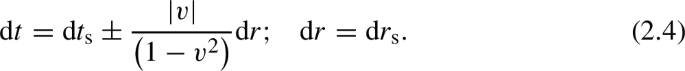
Here \(|v|=\sqrt{2M/r}\), and the \(+\) sign corresponds to a black hole spacetime and the − sign to its time reversal, i.e. a white hole.
One could also regain flat spatial slices by letting the flow vector vanishe \(\textbf{v} \rightarrow 0\), but that is uninteresting as it simply reduces to flat Minkowski space.

References
Painlevé, P.: La mécanique classique et la théorie de la relativité. C. R. Acad. Sci. (Paris) 173, 677–680 (1921)
Painlevé, P.: La gravitation dans la mécanique de Newton et dans la mécanique d’Einstein. C. R. Acad. Sci. (Paris) 173, 873–886 (1921)
Gullstrand, A.: Allgemeine Lösung des statischen Einkörperproblems in der Einsteinschen Gravitationstheorie. Arkiv för Matematik, Astronomi och Fysik. 16(8), 1–15 (1922)
Roy, K.: Gravitational field of a spinning mass as an example of algebraically special metrics. Phys. Rev. Lett. 11, 237–238 (1963). (Reprinted in [9])
Kerr, R.: “Gravitational collapse and rotation”. Published in: Quasi-stellar sources and gravitational collapse: Including the proceedings of the First Texas Symposium on Relativistic Astrophysics. Ivor Robinson, Alfred Schild, E.L. Schücking (eds.) University of Chicago Press, Chicago, pp. 99–102 (1965). The conference was held in Austin, Texas, on 16–18 December 1963. Reprinted in [9]
Kerr, R.: Discovering the Kerr and Kerr-Schild metrics. arXiv:0706.1109 [gr-qc]. Published in [9]
Newman, E., Couch, E., Chinnapared, K., Exton, A., Prakash, A., Torrence, R.: Metric of a rotating, charged mass. J. Math. Phys. 6, 918 (1965)
Visser, M.: The Kerr spacetime: a brief introduction. arXiv:0706.0622 [gr-qc]. Published in [9]
Wiltshire, D.L., Visser, M., Scott, S.M. (eds.): The Kerr Spacetime: Rotating Black Holes in General Relativity. Cambridge University Press, Cambridge (2009)
O’Neill, B.: The Geometry of Kerr Black Holes, (Peters, Wellesley, 1995). Mineloa, Reprinted (Dover (2014)
Martel, K., Poisson, E.: Regular coordinate systems for Schwarzschild and other spherical space-times. Am. J. Phys. 69, 476–480 (2001). https://doi.org/10.1119/1.1336836
Faraoni, V., Vachon, G.: When Painlevé-Gullstrand coordinates fail. Eur. Phys. J. C 80(8), 771 (2020). https://doi.org/10.1140/epjc/s10052-020-8345-4
Weinberg, S.: Gravitation and Cosmology: Principles and Applications of the General Theory of Relativity. Wiley, Hoboken (1972)
Misner, C., Thorne, K., Wheeler, J.A.: Gravitation. Freeman, San Francisco (1973)
Ronald, J., Adler, M.B., Schiffer, M.: Introduction to General Relativity, Second edition. McGraw–Hill, New York (1975). It is important to acquire the 1975 second edition, the 1965 first edition does not contain any discussion of the Kerr spacetime
Wald, R.: General Relativity. University of Chicago Press, Chicago (1984)
D’Inverno, R.: Introducing Einstein’s Relativity. Oxford University Press, Oxford (1992)
Hartle, J.: Gravity: An Introduction to Einstein’s General Relativity. Addison Wesley, San Francisco (2003)
Carroll, S.: An Introduction to General Relativity: Spacetime and Geometry. Addison Wesley, San Francisco (2004)
Hobson, M.P., Estathiou, G.P., Lasenby, A.N.: General Relativity: An Introduction for Physicists. Cambridge University Press, Cambridge (2006)
Poisson, E.: A Relativist’s Toolkit: The Mathematics of Black-Hole Mechanics. Cambridge University Press, Cambridge (2009). https://doi.org/10.1017/CBO9780511606601
Padmanabhan, T.: Gravitation: Foundations and Frontiers. Cambridge University Press, Cambridge (2010)
Teukolsky, S.A.: The Kerr Metric. Class. Quant. Gravit. 32(12), 124006 (2015). https://doi.org/10.1088/0264-9381/32/12/124006
Adamo, T., Newman, E.T.: The Kerr–Newman metric: a review. Scholarpedia 9, 31791 (2014). https://doi.org/10.4249/scholarpedia.31791
Heinicke, C., Hehl, F.W.: Schwarzschild and Kerr solutions of Einstein’s field equation-an introduction. Int. J. Mod. Phys. D 24(02), 1530006 (2014). https://doi.org/10.1142/S0218271815300062
Bambi, C.: Testing the Kerr black hole hypothesis. Mod. Phys. Lett. A 26, 2453–2468 (2011). https://doi.org/10.1142/S0217732311036929
Johannsen, T.: Sgr A* and General Relativity. Class. Quant. Gravit. 33(11), 113001 (2016). https://doi.org/10.1088/0264-9381/33/11/113001
Reynolds, C.S.: The spin of supermassive black holes. Class. Quant. Gravit. 30, 244004 (2013). https://doi.org/10.1088/0264-9381/30/24/244004
Bambi, C.: Astrophysical black holes: a compact pedagogical review. Annalen Phys. 530, 1700430 (2018). https://doi.org/10.1002/andp.201700430
Reynolds, C.S.: Observing black holes spin. Nature Astron. 3(1), 41–47 (2019). https://doi.org/10.1038/s41550-018-0665-z
Barausse, E., Berti, E., Hertog, T., Hughes, S.A., Jetzer, P., Pani, P., Sotiriou, T.P., Tamanini, N., Witek, H., Yagi, K., et al.: Prospects for fundamental physics with LISA. Gen. Relativ. Gravit. 52(8), 81 (2020). https://doi.org/10.1007/s10714-020-02691-1
Arnowitt, R.L., Deser, S., Misner, C.W.: “The Dynamics of general relativity’’, Originally published in “Gravitation: an introduction to current research’’, edited by Louis Witten (Wiley,: chapter 7, pp 227–265. Republished as: Gen. Relativ. Gravit. 40(2008), 1997–2027 (1962). https://doi.org/10.1007/s10714-008-0661-1
Gourgoulhon, E.: 3+1 formalism and bases of numerical relativity. Lecture Notes in Physics, vol. 846. Springer, Heidelberg (2012). https://doi.org/10.1007/978-3-642-24525-1. arXiv:gr-qc/0703035 [gr-qc]
Visser, M.: Heuristic approach to the Schwarzschild geometry. Int. J. Mod. Phys. D 14, 2051–2068 (2005). https://doi.org/10.1142/S0218271805007929
Gaur, R., Visser, M.: Cosmology in Painlevé-Gullstrand coordinates. JCAP 09, 030 (2022). https://doi.org/10.1088/1475-7516/2022/09/030
Volovik, G. E.: Painleve-Gullstrand coordinates for Schwarzschild-de Sitter spacetime (2022). arXiv:2209.02698 [gr-qc]
Thirring, H., Lense, J.: Über den Einfluss der Eigenrotation der Zentralkörper auf die Bewegung der Planeten und Monde nach der Einsteinschen Gravitationstheorie. Phys. Z. 19, 156–163 (1918). English translation: Mashhoon, B., Hehl, F.W., Theiss, D.S. On the gravitational effects of rotating masses: The Thirring-Lense papers. Gen. Relativ. Gravit. 16, 727–741 (1984). https://doi.org/10.1007/BF00762913
Pfister, H.: On the history of the so-called Lense–Thirring effect. http://philsci-archive.pitt.edu/archive/00002681/01/lense.pdf
Baines, J., Berry, T., Simpson, A., Visser, M.: Painleve-Gullstrand form of the Lense-Thirring spacetime. Universe 7(4), 105 (2021). https://doi.org/10.3390/universe704010
Baines, J., Berry, T., Simpson, A., Visser, M.: Killing tensor and Carter constant for Painlevé-Gullstrand form of Lense-Thirring spacetime. Universe 7(12), 473 (2021). https://doi.org/10.3390/universe7120473
Baines, J., Berry, T., Simpson, A., Visser, M.: Geodesics for Painlevé-Gullstrand form of Lense-Thirring spacetime. Universe 8(2), 115 (2022). https://doi.org/10.3390/universe8020115
Baines, J., Berry, T., Simpson, A., Visser, M.: Constant-\(r\) geodesics in the Painlevé-Gullstrand form of Lense-Thirring spacetime. Gen. Relativ. Gravit. 54(8), 79 (2022). https://doi.org/10.1007/s10714-022-02963-y
Santiago, J., Schuster, S., Visser, M.: Generic warp drives violate the null energy condition. Phys. Rev. D 105(6), 064038 (2022). https://doi.org/10.1103/PhysRevD.105.064038
Schuster, S., Santiago, J., Visser, M.: ADM mass in warp drive spacetimes. [arXiv:2205.15950 [gr-qc]]
Santiago, J., Schuster, S., Visser, M.: Tractor beams, pressor beams and stressor beams in general relativity. Universe 7(8), 271 (2021). https://doi.org/10.3390/universe7080271
Visser, M., Santiago, J., Schuster, S.: Tractor beams, pressor beams, and stressor beams within the context of general relativity. [arXiv:2110.14926 [gr-qc]]. (MG16 conference, Rome, July 2021.)
Valiente Kroon, J.A.: On the nonexistence of conformally flat slices in the Kerr and other stationary space-times. Phys. Rev. Lett. 92, 041101 (2004). https://doi.org/10.1103/PhysRevLett.92.041101
Valiente Kroon, J.A.: Asymptotic expansions of the Cotton-York tensor on slices of stationary space-times. Class. Quant. Gravit. 21, 3237–3250 (2004). https://doi.org/10.1088/0264-9381/21/13/009
Baines, J., Berry, T., Simpson, A., Visser, M.: Darboux diagonalization of the spatial 3-metric in Kerr spacetime. Gen. Relativ. Gravit. 53(1), 3 (2021). https://doi.org/10.1007/s10714-020-02765-0
Van Den Broeck, C.: A warp drive with reasonable total energy requirements. Class. Quant. Gravit. 16, 3973–3979 (1999). https://doi.org/10.1088/0264-9381/16/12/314
Van Den Broeck, C.: On the (im)possibility of warp bubbles. [arXiv:gr-qc/9906050 [gr-qc]]
Barceló, C., Liberati, S., and Visser, M.: Analogue gravity. Living Rev. Rel. 8, 12 (2005). https://doi.org/10.12942/lrr-2005-12
Visser, M.: Acoustic black holes: horizons, ergospheres, and Hawking radiation. Class. Quant. Gravit. 15, 1767–1791 (1998). https://doi.org/10.1088/0264-9381/15/6/024
Barceló, C., Liberati, S., Visser, M.: Analog gravity from Bose-Einstein condensates. Class. Quant. Gravit. 18, 1137 (2001). https://doi.org/10.1088/0264-9381/18/6/312
Visser, M.: Acoustic propagation in fluids: an unexpected example of Lorentzian geometry. [arXiv:gr-qc/9311028 [gr-qc]]
Barceló, C., Liberati, S., Visser, M.: Analog gravity from field theory normal modes? Class. Quant. Gravit. 18, 3595–3610 (2001). https://doi.org/10.1088/0264-9381/18/17/313
Visser, M., Barceló, C., Liberati, S.: Analog models of and for gravity. Gen. Relativ. Gravit. 34, 1719–1734 (2002). https://doi.org/10.1023/A:1020180409214
Jain, P., Weinfurtner, S., Visser, M., Gardiner, C.W.: Analogue model of a FRW universe in Bose-Einstein condensates: Application of the classical field method. Phys. Rev. A 76, 033616 (2007). https://doi.org/10.1103/PhysRevA.76.033616
Visser, M., Molina-París, C.: Acoustic geometry for general relativistic barotropic irrotational fluid flow. New J. Phys. 12, 095014 (2010). https://doi.org/10.1088/1367-2630/12/9/095014
Liberati, S., Visser, M., Weinfurtner, S.: Analogue quantum gravity phenomenology from a two-component Bose-Einstein condensate. Class. Quant. Gravit. 23, 3129–3154 (2006). https://doi.org/10.1088/0264-9381/23/9/023
Nielsen, A.B., Visser, M.: Production and decay of evolving horizons. Class. Quant. Gravit. 23, 4637–4658 (2006). https://doi.org/10.1088/0264-9381/23/14/006
Hamilton, A.J.S., Lisle, J.P.: The River model of black holes. Am. J. Phys. 76, 519–532 (2008). https://doi.org/10.1119/1.2830526
Doran, C.: A New form of the Kerr solution. Phys. Rev. D 61, 067503 (2000). https://doi.org/10.1103/PhysRevD.61.067503
Baines, J., Visser, M.: Physically motivated ansatz for the Kerr spacetime. arXiv:2207.09034 [gr-qc]
Rajan, D., Visser, M.: Global properties of physically interesting Lorentzian spacetimes. Int. J. Mod. Phys. D 25(14), 1650106 (2016). https://doi.org/10.1142/S0218271816501066
Baines, J., Berry, T., Simpson, A., Visser, M.: Unit-lapse versions of the Kerr spacetime. Class. Quant. Gravit. 38(5), 055001 (2021). https://doi.org/10.1088/1361-6382/abd071
Fagnocchi, S., Finazzi, S., Liberati, S., Kormos, M., Trombettoni, A.: Relativistic Bose–Einstein condensates: a new system for analogue models of gravity. New J. Phys. 12, 095012 (2010). https://doi.org/10.1088/1367-2630/12/9/095012
Giacomelli, L., Liberati, S.: Rotating black hole solutions in relativistic analogue gravity. Phys. Rev. D 96(6), 064014 (2017). https://doi.org/10.1103/PhysRevD.96.064014
Liberati, S., Schuster, S., Tricella, G., Visser, M.: Vorticity in analogue spacetimes. Phys. Rev. D 99(4), 044025 (2019). https://doi.org/10.1103/PhysRevD.99.044025
Liberati, S., Tricella, G., Visser, M.: Towards a Gordon form of the Kerr spacetime. Class. Quant. Gravit. 35(15), 155004 (2018). https://doi.org/10.1088/1361-6382/aacb75
Acknowledgements
MV was directly supported by the Marsden Fund, via a grant administered by the Royal Society of New Zealand. SL acknowledges funding from the Italian Ministry of Education and Scientific Research (MIUR) under the grant PRIN MIUR 2017-MB8AEZ.
Funding
Open access funding provided by Scuola Internazionale Superiore di Studi Avanzati - SISSA within the CRUI-CARE Agreement.
Author information
Authors and Affiliations
Corresponding author
Additional information
Publisher's Note
Springer Nature remains neutral with regard to jurisdictional claims in published maps and institutional affiliations.
This article belongs to a Topical Collection: In Memory of Professor T Padmanabhan.
Rights and permissions
Open Access This article is licensed under a Creative Commons Attribution 4.0 International License, which permits use, sharing, adaptation, distribution and reproduction in any medium or format, as long as you give appropriate credit to the original author(s) and the source, provide a link to the Creative Commons licence, and indicate if changes were made. The images or other third party material in this article are included in the article’s Creative Commons licence, unless indicated otherwise in a credit line to the material. If material is not included in the article’s Creative Commons licence and your intended use is not permitted by statutory regulation or exceeds the permitted use, you will need to obtain permission directly from the copyright holder. To view a copy of this licence, visit http://creativecommons.org/licenses/by/4.0/.
About this article

Cite this article
Visser, M., Liberati, S. Painlevé–Gullstrand coordinates versus Kerr spacetime geometry. Gen Relativ Gravit 54, 145 (2022). https://doi.org/10.1007/s10714-022-03025-z
Received:
Accepted:
Published:
DOI: https://doi.org/10.1007/s10714-022-03025-z