Multi-view and multi-augmentation for self-supervised visual representation learning

Abstract

In the real world, the appearance of identical objects depends on factors as varied as resolution, angle, illumination conditions, and viewing perspectives. This suggests that the data augmentation pipeline could benefit downstream tasks by exploring the overall data appearance in a self-supervised framework. Previous work on self-supervised learning that yields outstanding performance relies heavily on data augmentation such as cropping and color distortion. However, most methods use a static data augmentation pipeline, limiting the amount of feature exploration. To generate representations that encompass scale-invariant, explicit information about various semantic features and are invariant to nuisance factors such as relative object location, brightness, and color distortion, we propose the Multi-View, Multi-Augmentation (MVMA) framework. MVMA consists of multiple augmentation pipelines, with each pipeline comprising an assortment of augmentation policies. By refining the baseline self-supervised framework to investigate a broader range of image appearances through modified loss objective functions, MVMA enhances the exploration of image features through diverse data augmentation techniques. Transferring the resultant representation learning using convolutional networks (ConvNets) to downstream tasks yields significant improvements compared to the state-of-the-art DINO across a wide range of vision tasks and classification tasks: +4.1% and +8.8% top-1 on the ImageNet dataset with linear evaluation and k-NN classifier, respectively. Moreover, MVMA achieves a significant improvement of +5% $AP_{50}$ and +7% $AP_{50}^m$ on COCO object detection and segmentation.

Appendices

Appendix

A Implementation details

1.1 A.1 Implementation details of MVMA training

First, we provide a pseudo-code for MVMA self-supervised training loop in Pytorch style as shown in Algorithm 1.

Algorithm 1

MVMA’s main learning algorithm.

In our study, the MVMA self-supervised pretraining technique utilizes stochastic gradient descent across multiple instances, benefiting from large batch sizes. We allocate 2048 images for the ConvNet and 1024 images for the ViT, distributed across 16 A100 80Gb GPUs. Accordingly, each GPU processes 128 instances for the ConvNet and 64 for the ViT. For consistency, batch normalization across GPUs is synchronized using a kernel from the CUDA/C-v2 component of the NVIDIA Apex-2 library, which also supports mixed-precision training. Notably, MVMA proves more amenable to multi-node distribution than self-supervised contrastive techniques like SimCLR or MoCo, which often face bottlenecks due to feature matrix sharing across GPUs. With this setup, as illustrated in Fig. A.1, we monitor the linear evaluation performance on our method with different architecture scale and show the outstanding improvement over entire training process (we take BYOL as baseline).

Fig. 11

Performance gain during self-supervised pretraining. We track the improvement of the proposed method with different architecture setup (RN50 and Scaled RN50(x2)) over 100 training epoch and show the increasing improvement over BYOL baseline

Table 10 Detailed overview of augmentation operations

1.2 A.2 Implement of MVMA multi-data augmentation pipeline

In our MVMA multi-data augmentation process, we begin with the Random Resize Crop technique. We obtain two distinct global views of an image by using crops of varied sizes and aspect ratios. Specifically, we employ the RandomResizedCrop method from the torchvision.transforms module in PyTorch, using a crop ratio $s = (0.3, 1.0)$. Subsequently, these full-resolution views are resized to a standard dimension of $224 \times 224$ pixels. Additionally, we gather $V$ more local views (typically three to six in our experiments) using a crop ratio $s = (0.1, 0.3)$. The resultant crops are resized to $96 \times 96$ pixels. These cropped views then undergo transformations within our multi-augmentation pipeline. As explained in Section 3.2 from the main text, this pipeline involves combinations of 2 to 3 augmentation strategies tailored for both ConvNet and ViT architectures. Each strategy is comprised of many augmentation techniques. For a thorough understanding, Table 10 provides a comprehensive description of these techniques, transformation magnitude ranges, and the influence of potential variations on image transformation.

The specifics of each augmentation strategy are as follows:

• 1. SimCLR Augment: Each cropped view undergoes a series of image augmentations, which are composed of a specific sequence of transformations. These transformations include flipping, color distortion, grayscale conversion, gaussian blur, and solarization. A comprehensive description of these augmentations, including their respective probabilities, can be found in Table 11. The processing flow for each image is as follows:

  • 1. Optional horizontal flipping, allowing for left-to-right inversions;

  • 2. Color adjustments, where brightness, contrast, saturation, and hue undergo uniform shifts;

  • 3. An optional step to convert the RGB image to grayscale;

  • 4. Gaussian blurring using a $23 \times 23$ square kernel, with a standard deviation uniformly chosen from the range $[0.1, 2.0]$;

  • 5. Optional solarization, a pixel-wise color transformation defined as $x \mapsto x \cdot l_{(x<0.5)} + (1-x) \cdot l_{(x\ge 0.5)}$ for pixel values within the $[0, 1]$ interval.

• 6. Auto Augmentation: We used the searched policies specifically for the ImageNet based dataset. A detailed list of these policies is available in Table 12. These policies encompass 16 distinct operations, namely ShearX, ShearY, TranslateX, TranslateY, Rotate, AutoContrast, Invert, Equalize, Solarize, Posterize, Contrast, Color, Brightness, Sharpness, Cutout, and Sample Pairing. In this augmentation strategy, each cropped view is transformed from a chosen sub-policy, denoted as $\tau$. This sub-policy integrates two specific augmentation techniques. Every technique within $\tau$ is defined by two parameters: the likelihood i of invoking the operation and the magnitude $\lambda$ associated with the operation.

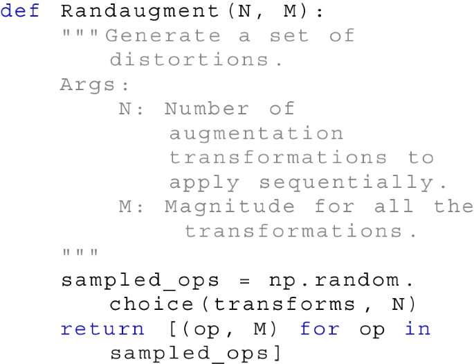
• 7. Expand RandAugment: Each cropped view apply through a sequence of $N$ transformations, selected randomly with a uniform probability of $1/K$, where $K$ represents the total number of transformations available in our Expand RandAugment k=18. The selected transformations in our list comprise: [GaussianNoise, AutoContrast, rand_hue, Affine, CoarseDropout, Equalize, Invert, rand_brightness, Posterize, Solarize, Sharpness, SolarizeAdd, Sharpen, Color, FastSnowyLandscape, Rain, rand_saturation, EdgeDetect]. For each of the $N$ transformations, a corresponding magnitude is randomly selected and applied. We utilize a consistent linear scale to denote the intensity of each transformation, aligning it with its predefined minimum and maximum range values. The implementation of this approach is characterized by two primary parameters: $N$ and $M$. This can be succinctly represented in Python as:

  

• 8. Fast AutoAugment: Each cropped view transform through a designated sub-policy. This sub-policy is derived from a set of searched policies, which are informed by a comprehensive search space encompassing 17 distinct operations. These operations include [ShearX, ShearY, TranslateX, TranslateY, Rotate, AutoContrast, Invert, Equalize, Solarize, Posterize, Contrast, Color, Brightness, Sharpness, Cutout, Sample Pairing, Flip ]. A comprehensive list of the searched policies, specifically adapted for the ImageNet dataset, can be found in Table 13. Similar to AutoAugment approach, each sub-policy, denoted as $\tau$, incorporates two distinct augmentation techniques. For example, $\tau$ the sub-policy 0 consist of [Contrast, Translate]. Every transformation within $\tau$ is characterized by two parameters: the likelihood i of executing the operation and the magnitude $\lambda$ associated with that operation.

Table 11 A detailed of SimCLR’s augmentation pipeline

Table 12 AutoAugment policy searched on reduced ImageNet

In our experiments with the ConvNet architecture, as discussed in Section 5.3 in the main text, we observed that combining three augmentation strategies yielded the best results when pretraining in a self-supervised mode using only two global views. Specifically, for ConvNet (ResNet-50), a mix of SimCLR, RandAugment, and Auto Augmentation strategies proved to be most effective. However, when we included multi-cropping views, only the SimCLR and RandAugment strategies were necessary. For the Vision Transformer model, our data indicated its extensive data needs. Employing multiple data augmentation strategies effectively addressed this, with combinations of 3 to 4 strategies consistently producing the best outcomes, irrespective of the view type (global or multi-views).

Table 13 Fast AutoAugmentation policy searched on ImageNet

B Transferring obtained learned features to downstream tasks

To assess the efficacy of our MVMA transfer learning across varied datasets and tasks, we adopted standard evaluation metrics. Each dataset is characterized by distinct metrics, ensuring that our results are both comparable and consistent. The metrics we employed are detailed as follows:

• Top-1 Accuracy: This metric quantifies the percentage of instances that the model correctly classified.

• Mean Per Class Accuracy: Here, the accuracy for each class is calculated individually. Subsequently, the average of these individual accuracies offers an overarching assessment.

• Average Precision (AP): AP denotes the Average Precision, signifying the area under the precision-recall curve.

• AP50 and AP75: These metrics correspond to AP values determined at specific IoU (Intersection over Union) thresholds. Specifically, AP50 is gauged at an IoU threshold of 0.5, while AP75 is evaluated at a threshold of 0.75.

• Euclidean Distance: Predominantly utilized in the context of the K-NN algorithm, this metric measures distance between two real-valued vectors, especially when pinpointing the K nearest neighbors of a query point.

• Mean Region Similarity ($\mathcal {J}_m$): This metric evaluates the likeness between the predicted and the actual segmentation masks, relying on the intersection over union methodology.

• Mean Contour-Based Accuracy ($\mathcal {F}_m$): Here, the precision of predicted object boundaries is gauged using the F-measure, a metric that harmonizes both precision and recall.

• Average Score ($\mathcal {J} \& \mathcal {F}$): Representing a composite metric, this is the average of the $\mathcal {J}_m$ and $\mathcal {F}_m$ scores, offering insights into both region similarity and boundary accuracy.

1.1 B.1 Evaluation on the ImageNet

Data preprocessing for our experiments involves the following steps: During training, we employ basic augmentation techniques on the images, such as random flips and resizing to 224x224 pixels. In the testing phase, we resize all images to 256 pixels on the shorter edge with bicubic resampling and extract a 224x224 center crop. All images are normalized per color channel both during training and testing, using statistics derived from the ImageNet dataset [41].

Linear evaluation

Without altering the network parameters and batch statistics, we train a linear classifier using the representation from the frozen pre-trained encoder. Adhering to the standard protocol for ImageNet, as referenced in [5], we employ the SGD optimizer with Nesterov momentum to minimize the cross-entropy loss over 100 epochs, utilizing a batch size of 1024 and a momentum of 0.9. Our results are based on the test set accuracy, specifically from the ILSVRC2012 ImageNet’s public validation set [41].

Table 14 Specification of 7 Natural Image Datasets

ImageNet K-NN evaluation

To assess the quality of unsupervised featuresrepresentations produced by the ResNet-50 and ViT-small models pre-trained with MVMA, we employed the k-NN evaluation method, as delineated in prior studies [6]. Initially, representations were extracted from the pre-trained model, eschewing any form of data augmentation. Subsequent classification was conducted using a weighted k-NN method, leveraging the cyanure library [55]. This k-NN classifier allocated labels to image features based on a voting mechanism that considered the k closest archived features. Notably, k-NN classifiers offer the distinct advantage of rapid deployment coupled with minimal resource overhead, negating the necessity for domain adaptation. Through systematic experimentation with various k values, we discerned that a value of 20 yielded consistently superior outcomes. This evaluation paradigm is characterized by its simplicity, necessitating only marginal hyperparameter fine-tuning and a singular traversal of the downstream dataset.

1.2 B.2 Transfer via linear classification and fine-tuning

Datasets

Following prior studies [5, 15], we transfer the representation for linear classification and fine-tune on six diverse natural image datasets: Food-101 [56], CIFAR-10 [57], CIFAR-100 [57], SUN397 [58], Stanford Cars [59], Describable Textures Dataset (DTD) [60], and the Oxford-IIIT Pets [61]. Details for each dataset can be found in Table 14.

Transfer linear classification

Keeping the network parameters of the pre-trained encoder frozen, we adhere to the standard linear evaluation protocol as in [5]. During both training and testing, images are resized to 224x224 and normalized using ImageNet statistics, eschewing additional data augmentation. Image normalization involves channel-wise subtraction of mean colors and division by the standard deviation. A logistic regression classifier, regularized using l2, is trained atop the static representation. We adjust the l2 regularization from a logarithmically spaced set of 45 values between $10^{-6}$ and $10^{5}$, aligning with the optimization process in[5]. Post-training, accuracy is gauged on the test set.

Transfer fine-tuning

We follow fine-tuning protocol as in [5] to initialize the network with the parameters of the pre-trained representation. At both phase training and testing time, we follow the image preprocessing and data augmentation strategies from the procedure in ImageNet linear evaluation setting. To fine-tune the network, we optimized the cross-entropy loss using SGD optimizer with a Nesterov momentum value of 0.9 and trained over 60 epochs with a batch size of 256. We set a hyperparameter including the momentum parameter for batch statistics, learning rate, and weight decay selection method, same as in [5]. After selecting the optimal hyperparameters configured on the validation set, the model is retrained on the combined train and validation set together, using the specified parameters. The absolute accuracy is reported on the test set.

Object detection and segmentation

We explore the generalization and robustness of the learned representations of our ConvNet architecture, leveraging a standard ResNet-50, and a Vision Transformer (ViT) model, specifically the standard ViT-S. Both models are initially with self-supervised pretrained on ImageNet using MVMA framework. They are subsequently repurposed for object detection and instance segmentation tasks on the COCO dataset via fine-tuning, employing the Detectron2 [45] framework. We use Mask R-CNN [46] based architecture for both ViT and ConvNet to fine-tuned on COCO train2017 and evaluated on val2017 With respect to the ConvNet (ResNet) model, we incorporate a Feature Pyramid Network (FPN) [47] into the Mask R-CNN [46], creating the R50-FPN backbone configuration. The BatchNorm layer is fine-tuned in line with Detectron2 guidelines. Training images are scaled within a range of 640 to 800 pixels, while a consistent scale of 800 pixels is applied during inference. We perform end-to-end fine-tuning of the model on the train2017 set, which comprises approximately 118,000 images, and evaluate performance using the val2017 set. We adopt the 1x (about 12 epochs) or 2x schedule from the original Mask R-CNN paper for training. However, it should be noted that the suitability of these schedules may be limited due to recent advancements in the field. The initial learning rate is set at 0.003. Training is conducted over 90,000 iterations on single A100 80GB GPUs with a batch size of 26. After the 60,000th and 80,000th iterations, the learning rate is decreased by a factor of 10. We utilize SyncBatchNorm to fine-tune BatchNorm parameters and incorporate an additional BatchNorm layer following the res5 layer, in accordance with the Res5ROIHeadsExtraNorm head in Detectron2.

For the Vision Transformer (ViT) model, we follow the default training recipe outlined in the original paper [49], adapting it for Mask R-CNN usage. The stack of transformer blocks in ViT, all of which yield feature maps at a single scale, is partitioned into four subsets. Convolutions are then applied to manipulate the scale of the intermediate feature maps, thereby creating multi-scale maps. These maps facilitate the construction of an FPN head. Detailed architectural adaptations are delineated in Appendix A.2 of the referenced paper [49]. Our default training setting with an input size of 1024x1024 pixels. Training is supplemented by large-scale jitter, with a scale range of 0.1 to 2.0. We employ the AdamW optimizer ($\beta _1, \beta _2 = 0.9, 0.999$) with step-wise learning rate decay. The initial learning rate is set at 0.1, with a linear learning rate warm-up phase implemented for the first 50k iterations. The training process is in one A100 80GB GPUs with a batch size of 26.

Finally, we present the results of object detection and instance segmentation tasks, following fine-tuning on the COCO dataset. The evaluation incorporates widely accepted detection and segmentation metrics, including bounding box Average Precision (AP, $AP_{50}$, and $AP_{75}$) and mask Average Precision ($AP_{50}^m$, $AP^m$, and $AP_{75}^m$).

References

Misra I, van der Maaten L (2020) Self-supervised learning of pretext-invariant representations. In: Proceedings of the IEEE/CVF conference on computer vision and pattern recognition, pp 6707–6717
Goyal P, Caron M, Lefaudeux B, Xu M, Wang P, Pai V, Singh M, Liptchinsky V, Misra I, Joulin A et al (2021) Self-supervised pretraining of visual features in the wild. arXiv preprint arXiv:2103.01988
Ermolov A, Siarohin A, Sangineto E, Sebe N (2021) Whitening for self-supervised representation learning. In: International conference on machine learning, pp 3015–3024. PMLR
Caron M, Misra I, Mairal J, Goyal P, Bojanowski P, Joulin A (2020) Unsupervised learning of visual features by contrasting cluster assignments. Adv Neural Inf Process Sys 33:9912–9924
Chen T, Kornblith S, Norouzi M, Hinton G (2020) A simple framework for contrastive learning of visual representations. In: International conference on machine learning, pp 1597–1607. PMLR
Caron M, Touvron H, Misra I, Jégou H, Mairal J, Bojanowski P, Joulin A (2021) Emerging properties in self-supervised vision transformers. In: Proceedings of the IEEE/CVF international conference on computer vision, pp 9650–9660
Hjelm RD, Fedorov A, Lavoie-Marchildon S, Grewal K, Bachman P, Trischler A, Bengio Y (2018) Learning deep representations by mutual information estimation and maximization. arXiv preprint arXiv:1808.06670
Zhao Z, Zhang Z, Chen T, Singh S, Zhang H (2020) Image augmentations for gan training. arXiv preprint arXiv:2006.02595
Gidaris S, Singh P, Komodakis N (2018) Unsupervised representation learning by predicting image rotations. arXiv preprint arXiv:1803.07728
Szegedy C, Liu W, Jia Y, Sermanet P, Reed S, Anguelov D, Erhan D, Vanhoucke V, Rabinovich A (2015) Going deeper with convolutions. In: Proceedings of the IEEE conference on computer vision and pattern recognition, pp 1–9
Howard AG (2013) Some improvements on deep convolutional neural network based image classification. arXiv preprint arXiv:1312.5402
Cubuk ED, Zoph B, Mane D, Vasudevan V, Le QV (2019) Autoaugment: Learning augmentation strategies from data. In: Proceedings of the IEEE/CVF conference on computer vision and pattern recognition, pp 113–123
Cubuk ED, Zoph B, Shlens J, Le QV (2020) Randaugment: Practical automated data augmentation with a reduced search space. In: Proceedings of the IEEE/CVF conference on computer vision and pattern recognition workshops, pp 702–703
Lim S, Kim I, Kim T, Kim C, Kim S (2019) Fast autoaugment. Adv Neural Inf Process Sys 32
Grill JB, Strub F, Altché F, Tallec C, Richemond P, Buchatskaya E, Doersch C, Pires BA, Guo Z, Azar MG et al (2020) Bootstrap your own latent-a new approach to self-supervised learning. Advances Neural Inf Process Sys 33:21271–21284
He K, Fan H, Wu Y, Xie S, Girshick R (2020) Momentum contrast for unsupervised visual representation learning. In: Proceedings of the IEEE/CVF conference on computer vision and pattern recognition, pp 9729–9738
Bromley J, Guyon I, LeCun Y, Säckinger E, Shah R (1993) Signature verification using a” siamese” time delay neural network. Adv Neural Inf Process Sys 6
Chopra S, Hadsell R, LeCun Y (2005) Learning a similarity metric discriminatively, with application to face verification. In: 2005 IEEE Computer society conference on computer vision and pattern recognition (CVPR’05) vol 1, pp 539–546. IEEE
van den Oord A, Li Y, Vinyals O (2018) Representation learning with contrastive predictive coding. arXiv preprint arXiv:1807.03748
Caron M, Bojanowski P, Joulin A, Douze M (2018) Deep clustering for unsupervised learning of visual features. In: Proceedings of the European conference on computer vision (ECCV), pp 132–149
Zbontar J, Jing L, Misra I, LeCun Y, Deny S (2021) Barlow twins: Self-supervised learning via redundancy reduction. In: International conference on machine learning, pp 12310–12320. PMLR
Richemond PH, Grill JB, Altché F, Tallec C, Strub F, Brock A, Smith S, De S, Pascanu R, Piot B et al (2020) Byol works even without batch statistics. arXiv preprint arXiv:2010.10241
Chen X, He K (2021) Exploring simple siamese representation learning. In: Proceedings of the IEEE/CVF conference on computer vision and pattern recognition, pp 15750–15758
Devlin J, Chang MW, Lee K, Toutanova K (2019) Bert: Pre-training of deep bidirectional transformers for language understanding. ArXiv arXiv:1810.04805
He K, Chen X, Xie S, Li Y, Doll’ar P, Girshick RB (2021) Masked autoencoders are scalable vision learners. IEEE/CVF Conference on computer vision and pattern recognition (CVPR) 2022:15979–15988
Xie Z, Zhang Z, Cao Y, Lin Y, Bao J, Yao Z, Dai Q, Hu H (2021) Simmim: a simple framework for masked image modeling. IEEE/CVF Conference on computer vision and pattern recognition (CVPR) 2022:9643–9653
Bao H, Dong L, Wei F (2021) Beit: Bert pre-training of image transformers. ArXiv arXiv:2106.08254
Zhou J, Wei C, Wang H, Shen W, Xie C, Yuille AL, Kong T (2021) ibot: Image bert pre-training with online tokenizer. ArXiv arXiv:2111.07832
Oquab M, Darcet T, Moutakanni T, Vo HQ, Szafraniec M, Khalidov V, Fernandez P, Haziza D, Massa F, El-Nouby A, Assran M, Ballas N, Galuba W, Howes R, Huang P-Y (Bernie), Li S-W, Misra I, Rabbat MG, Sharma V, Synnaeve G, Xu H, Jégou H, Mairal J, Labatut P, Joulin A, Bojanowski P (2023) Dinov2: Learning robust visual features without supervision. ArXiv arXiv:2304.07193
Chen X, Ding M, Wang X, Xin Y, Mo S, Wang Y, Han S, Luo P, Zeng G, Wang J (2022) Context autoencoder for self-supervised representation learning. ArXiv arXiv:2202.03026
Chen Y, Liu Y, Jiang D, Zhang X, Dai W, Xiong H, Tian Q (2022) Sdae: Self-distillated masked autoencoder. In: European conference on computer vision
Tran VN, Huang C-E, Liu S-H, Yang K-L, Ko T, Li Y-H (2022) Multi-augmentation for efficient self-supervised visual representation learning. In: 2022 IEEE International Conference on Multimedia and Expo Workshops (ICMEW), pp 1–4
Krizhevsky A, Sutskever I, Hinton GE (2017) Imagenet classification with deep convolutional neural networks. Commun ACM 60(6):84–90
Touvron H, Vedaldi A, Douze M, Jégou H (2019) Fixing the train-test resolution discrepancy. Adv Neural Inf Process Sys 32
Jones DR (2001) A taxonomy of global optimization methods based on response surfaces. J Glob Optim 21:345–383
Reed CJ, Metzger S, Srinivas A, Darrell T, Keutzer K (2021) Selfaugment: Automatic augmentation policies for self-supervised learning. In: Proceedings of the IEEE/CVF conference on computer vision and pattern recognition, pp 2674–2683
He K, Zhang X, Ren S, Sun J (2016) Deep residual learning for image recognition. In: Proceedings of the IEEE conference on computer vision and pattern recognition, pp 770–778
Dosovitskiy A, Beyer L, Kolesnikov A, Weissenborn D, Zhai X, Unterthiner T, Dehghani M, Minderer M, Heigold G, Gelly S et al (2020) An image is worth 16x16 words: Transformers for image recognition at scale. arXiv preprint arXiv:2010.11929
Ioffe S, Szegedy C (2015) Batch normalization: Accelerating deep network training by reducing internal covariate shift. In: International conference on machine learning
Agarap AF (2018) Deep learning using rectified linear units (relu). ArXiv arXiv:1803.08375
Russakovsky O, Deng J, Su H, Krause J, Satheesh S, Ma S, Huang Z, Karpathy A, Khosla A, Bernstein M et al (2015) Imagenet large scale visual recognition challenge. Int J Comput Vis 115:211–252
Goyal P, Dollár P, Girshick R, Noordhuis P, Wesolowski L, Kyrola A, Tulloch A, Jia Y, He K (2017) Accurate, large minibatch sgd: Training imagenet in 1 hour. arXiv preprint arXiv:1706.02677
Loshchilov I, Hutter F (2017) Fixing weight decay regularization in adam. ArXiv arXiv:1711.05101
Loshchilov I, Hutter F (2016) Sgdr: Stochastic gradient descent with warm restarts. arXiv preprint arXiv:1608.03983
Wu Y, Kirillov A, Massa F, Lo W-Y, Girshick R (2019) Detectron2. https://github.com/facebookresearch/detectron2
He K, Gkioxari G, Dollár P, Girshick R (2017) Mask r-cnn. In: Proceedings of the IEEE international conference on computer vision, pp 2961–2969
Lin T-Y, Dollár P, Girshick R, He K, Hariharan B, Belongie S (2017) Feature pyramid networks for object detection. In: Proceedings of the IEEE conference on computer vision and pattern recognition, pp 2117–2125
Girshick R, Radosavovic I, Gkioxari G, Dollár P, He K (2018) Detectron. https://github.com/facebookresearch/detectron
Li Y, Mao H, Girshick RB, He K (2022) Exploring plain vision transformer backbones for object detection. ArXiv arXiv:2203.16527
Chen X, Xie S, He K (2021) An empirical study of training self-supervised vision transformers. In: Proceedings of the IEEE/CVF international conference on computer vision, pp 9640–9649
Pont-Tuset J, Perazzi F, Caelles S, Arbeláez P, Sorkine-Hornung A, Van Gool L (2017) The 2017 davis challenge on video object segmentation. arXiv preprint arXiv:1704.00675
Jabri A, Owens A, Efros A (2020) Space-time correspondence as a contrastive random walk. Adv Neural Inf Process Sys 33:19545–19560
Selvaraju RR, Cogswell M, Das A, Vedantam R, Parikh D, Batra D (2017) Grad-cam: Visual explanations from deep networks via gradient-based localization. In: Proceedings of the IEEE international conference on computer vision, pp 618–626
Tran VN, Liu S-H, Li Y-H, Wang J-C (2022) Heuristic attention representation learning for self-supervised pretraining. Sensors 22(14)
Mairal J (2019) Cyanure: An open-source toolbox for empirical risk minimization for python, c++, and soon more. ArXiv arXiv:1912.08165
Bossard L, Guillaumin M, Van Gool L (2014) Food-101 - mining discriminative components with random forests. In: European conference on computer vision
Krizhevsky A (2009) Learning multiple layers of features from tiny images
Xiao J, Hays J, Ehinger KA, Oliva A, Torralba A (2010) Sun database: Large-scale scene recognition from abbey to zoo. IEEE Computer society conference on computer vision and pattern recognition 2010:3485–3492
Krause J, Stark M, Deng J, Fei-Fei L (2013) 3d object representations for fine-grained categorization. IEEE International conference on computer vision workshops 2013:554–561
Tzimiropoulos G, Pantic M (2016) 2014 gauss-newton deformable part models for face alignment in-the-wild. In: 2014 IEEE Conference on computer vision and pattern recognition, 23-28 June 2014, Columbus, USA
Parkhi OM, Vedaldi A, Zisserman A, Jawahar CV (2012) Cats and dogs. IEEE Conference on computer vision and pattern recognition 2012:3498–3505
Author information
Authors and Affiliations
Contributions
The authors of the research paper made significant contributions to the study. Yung-Hui Li provided the methodology and conceptualized the study, while Chi-En Huang, Van Nhiem Tran, and Shen-Hsuan Liu developed and validated the software. Kai-Lin Yang assisted with data curation. Muhammad Saqlain Aslam, Van Nhiem Tran, Chi-En Huang, Shen-Hsuan Liu, and Yung-Hui Li contributed to writing, reviewing, and editing. Yung-Hui Li and Jia-Ching Wang provided supervision, and Yung-Hui Li also managed project administration and acquired funding. All authors have approved the published work.
Corresponding author
Ethics declarations
Informed Consent
Not applicable.
Conflict of Interest
The authors declare that they have no conflict of interest.
Additional information
Publisher's Note
Springer Nature remains neutral with regard to jurisdictional claims in published maps and institutional affiliations.