
Abstract
This paper is about the application of optimization methods to the analysis of three pricing schemes adopted by one manufacturer in a two-country model of production and trade. The analysis focuses on pricing schemes—one uniform pricing scheme, and two differential pricing schemes—for which there is no competition coming from the so-called parallel trade. This term denotes the practice of buying a patented product like a medicine in one market at one price, then re-selling it in a second so-called gray market at a higher price, on a parallel distribution chain where it competes with the official distribution chain. The adoption of pricing schemes under which parallel trade does not arise can prevent the occurrence of its well-documented negative effects. In the work, a comparison of the optimal solutions to the optimization problems modeling the three pricing schemes is performed. More specifically, conditions are found under which the two differential pricing schemes are more desirable from several points of view (e.g., incentive for the manufacturer to do Research and Development, product accessibility, global welfare) than the uniform pricing scheme. In particular, we prove that, compared to the uniform pricing scheme, the two differential pricing schemes increase the incentive for the manufacturer to invest in Research and Development. We also prove that they serve both countries under a larger range of values for the relative market size, making the product more accessible to consumers in the lower price country. Moreover, we provide a sufficient condition under which price discrimination is more efficient from a global welfare perspective than uniform pricing. The analysis applies in particular to the case of the European Single Market for medicines. Compared to other studies, our work takes into account also the possible presence in all the optimization problems of a positive constant marginal cost of production, showing that it can have non-negligible effects on the results of the analysis. As an important contribution, indeed, our analysis clarifies the conditions—which have been overlooked in the literature about the mechanisms adopted to prevent parallel trade occurrence—that allow/do not allow one to neglect the presence of this factor. Such conditions are related, e.g., to the comparison between the positive constant marginal cost of production, the parallel trade cost per-unit, and the maximal price that can be effectively charged to the consumers in the lower price country.
1 Introduction
Drug prices, transaction costs, and regulations usually vary across countries, even for the same medicine. Under suitable conditions, if a patented drug is sold in at least two countries, differences in such factors may create an arbitrage opportunity even before patent expiration, providing an incentive to the emergence of so-called gray markets (Scott Morton and Kyle 2012). This phenomenon (which is also referred to in the literature as parallel tradeFootnote 1, see Danzon 1998) consists in the practice of buying a patented product at one price in one country, then re-selling it at a higher price in a second country, on a parallel distribution chain where it competes with the official distribution chain. Different regulations at a national level may make this price heterogeneity last in time, possibly generating several inefficiencies, as highlighted in various theoretical and empirical works, such as Danzon (1998), Danzon and Towse (2003), Danzon et al. (2015), Duso et al. (2014), Gnecco et al. (2018), Kanavos et al. (2011), Li and Robles (2006), Maskus and Ganslandt (2002) and Towse et al. (2015). For instance, when parallel trade is legally permitted by policymakers, such heterogeneity may allow parallel traders (e.g., distributors or agents trading with authorized distributors) to obtain a profit from parallel trade itself, representing a serious threat to the investments of the manufacturers in Research and Development (R&D).Footnote 2 As a consequence, the analysis and the optimization of pricing schemes for which parallel trade does not occur (hence, for which its well-documented negative effects are not expected to arise) is a relevant research topic.Footnote 3 In this context, it is important to distinguish between uniform pricing schemes (under which manufacturers set the same price in different countries), and suitable differential pricing (or price discrimination) schemes (which allow manufacturers to set even a different price in each country, taking into account its specific features).
Contributions of the work Given this framework, in this paper, we investigate three specific pricing schemes—a uniform pricing scheme, and two differential pricing schemes—for which parallel trade does not occur, either because it is prohibited, or as a consequence of the strategy adopted by the manufacturer. Then, for a two-country model of production and trade, we evaluate and compare their global welfare effects, and the associated manufacturer’s incentive to invest in R&D. In the uniform pricing scheme considered in the paper (which was studied, in a less general setting, in other works, e.g., in Müller-Langer (2009b), where the marginal cost of production was neglected), the manufacturer sets the same drug price in both countries, making parallel trade unprofitable. Then, the common price is optimized. Conversely, in the case of differential pricing, the manufacturer has the opportunity of choosing different prices in the two countries. The two differential pricing schemes investigated in the paper refer, respectively, to the case in which parallel trade is legally forbidden, and to the one in which the manufacturer sets a price difference lower than or equal to a positive parallel trade cost per-unit,Footnote 4 in case it decides to serve both countries. In this way, potential parallel traders are discouraged.
Our analysis is mainly based on constrained quadratic optimization techniques applied to pricing. The optimization problems we solve (in closed form) take into account, at the same time, the marginal cost of production, the parallel trade cost per-unit (only for one model, in which its knowledge is needed), the decision whether to invest or not in R&D, and the total fixed cost of R&D. In contrast, other models in the literature (for instance, Maskus and Chen 2004; Müller-Langer 2009b) neglect some of the above-mentioned factors (e.g., the presence of a positive constant marginal cost of production), in order to simplify the resulting optimization problems. Taking into account such factors can be useful to assess the robustness of the conclusions obtained from the analysis of these models with respect to changes in their assumptions.
The main qualitative economic insights obtained from our analysis can be summarized as follows: for the specific model of production and trade considered in the paper (which, differently from most specialized literature, takes into account the possible presence of a positive constant marginal cost of production), we
-
1.
extend the pricing analysis done in previous studies, e.g., highlighting the influence of a positive constant marginal cost of production on the optimal strategies of the manufacturer (hence, also on the optimal prices, quantities, and surpluses), under the three different pricing schemes (see Propositions 2, 3, and 4, and the respective Corollaries 2, 3, and 4);
-
2.
clarify the conditions that allow/do not allow one to neglect in the analysis the presence of a positive constant marginal cost of production. Such conditions are related, e.g., to the comparison between the positive constant marginal cost of production, the parallel trade cost per-unit, and the maximal price that can be effectively charged to the consumers in the lower price country (see Remark 3 in the appendix for details);
-
3.
take into account the additional possibility for the manufacturer in the various pricing schemes (particularly, in the uniform pricing scheme and in the second differential pricing scheme) to decide not to serve one of the two countries. This splits effectively the corresponding optimization problem into three optimization subproblems (see Sects. 5.1, 5.2, 5.3);
-
4.
prove (by an analysis of the optimal prices) that the second differential pricing scheme, for which the manufacturer sets the price difference between the two countries to be sufficiently low to prevent parallel trade occurrence, is a “hybrid” between the uniform pricing scheme and the first differential pricing scheme, for which parallel trade is forbidden (see Remark 2, and Corollaries 2, 3, and 4 in the appendix);
-
5.
prove that, at optimality, the two differential pricing schemes increase the manufacturer’s incentive to invest in R&D with respect to the uniform pricing scheme, and quantify such incentive for the three cases (see Proposition 5);
-
6.
prove that, at optimality, for some choices of the model parameters, compared to the uniform pricing scheme, the two differential pricing schemes serve both countries under a larger range of values for the relative market size of the two countries. This is important from a society’s wellbeing perspective, because in this way the product becomes more accessible to consumers in the lower price country. For two pricing schemes, suitable marginal cost-dependent thresholds on the relative market size are identified, above which the lower price country is not served at optimality (see Proposition 6(i));
-
7.
prove that for some other choices of the model parameters, differential pricing schemes are more efficient at optimality than the uniform pricing scheme from a global welfare perspective. Suitable marginal cost-dependent ranges of values for the relative market size for which this occurs are also identified (see Proposition 6(ii)).
Possible policy implications are discussed in Sect. 6 (where the pricing schemes are compared at optimality in terms of manufacturer’s surplus, accessibility of the product in the two countries, global welfare, and loss of efficiency with respect to an idealized situation) and in the final section, where possible developments and extensions to game-theoretic models are also discussed.
Organization of the work The paper is organized as follows. Section 2 provides a literature review on the mostly negative effects of parallel trade, and on possible ways to prevent its occurrence. Section 3 presents the two-country model of production and trade used in the analysis. In Sect. 4, we express in closed form the optimal value of the global welfare for the two countries, solving a suitable quadratic optimization problem. Then, in Sect. 5 we find the corresponding value of the global welfare obtained when the manufacturer applies at optimality, respectively, the uniform pricing scheme and the two differential pricing schemes (solving other quadratic optimization problems). In Sect. 6, we compare the three pricing schemes at optimality, focusing on sufficient conditions under which the two differential pricing schemes dominate the uniform pricing one. Finally, Sect. 7 concludes the paper and discusses possible extensions. All the proofs are reported in Appendix A. Due to their length, the expressions of the optimal prices and quantities for the various models appear in Appendix B. Some technical remarks about the various models considered are reported in Appendix C. All these appendices may be skipped at a first reading of the article.
2 Literature review
In the literature, there is a strong debate about the opportunity of permitting or not parallel trade, and on its effects on the global welfare of the countries involved (Danzon 1998; Jelovac and Bordoy 2005; Li and Robles 2006). This is motivated by the fact that, on one side, manufacturers see parallel trade as a serious threat to their investments in R&D, whereas, on the other side, parallel trade can induce price convergence in the different countries, e.g., by decreasing prices in re-importing countries, where pharmaceuticals are more expensive (Towse 1998).Footnote 5 This was empirically confirmed, e.g., in Ganslandt and Maskus (2004), where it was found that the prices of drugs subject to competition from parallel trade fell relative to those of other drugs by 12–19%. Hence, the former products turned out to be more accessible to consumers (this is important from a society’s wellbeing perspective). On the other hand, in Duso et al. (2014), the reduction of the manufacturers’ incentive for product innovation was confirmed empirically (referring to the case of the German market of oral anti-diabetics) through a structural approach, by comparing a counterfactual scenario with the status quo market. In contrast, it was confirmed empirically that this incentive tends to increase as the market size gets larger (Acemoglu and Linn 2004). This issue is particularly relevant, since endogenous sunk costs, such as those associated with R&D, can improve the product quality, raising its demand (Sutton 1998). Another negative consequence of parallel trade is the associated increase in the risk of drug shortage, for all the countries involved, limiting patients’ access to drugs.
According to the analysis presented in Danzon (1998), trade usually increases global welfare, when it makes consumers in higher price countries benefit from lower prices in other countries, and such lower prices are motivated by a better technology. Nevertheless, in the case of pharmaceuticals, lower prices are often the result of a more intensive regulation, not of lower production costs. Hence, parallel trade of pharmaceuticals is expected to reduce global welfare in strictly regulated markets. According to Kanavos et al. (2011), another negative aspect of parallel trade is that most of the revenues it originates are accrued not to the consumers, but to the parallel traders themselves. It is also worth mentioning that, following Jelovac and Bordoy (2005), parallel trade may even positively affect global welfare, e.g., when it implies a reallocation of consumption from individuals with relatively less drug needs to individuals with relatively more such needs. Nevertheless, still according to Jelovac and Bordoy (2005), parallel trade decreases global welfare when it implies, instead, a reallocation of consumption from individuals with relatively more drug needs to individuals with relatively less such needs, and also when one market is not served due to parallel trade. Concluding, the effect of parallel trade on global welfare is considered in Jelovac and Bordoy (2005) to be ambiguous, in the sense that its positive/negative influence on global welfare often depends on which issues are taken into account in the model (e.g., the need for the manufacturer to recover from the cost of R&D).
Since parallel traders and manufacturers can be modeled as different agents with their own objectives, it is natural to investigate parallel trade using noncooperative game-theoretic models (Chen and Maskus 2005; Guo et al. 2013; Maskus and Chen 2004; Müller-Langer 2012). As an example, according to the two-country model presented in Maskus and Chen (2004), forbidding parallel trade is always advantageous from the manufacturer’s point of view, even though the effect of such a prohibition on the global welfare of the two countries is ambiguous (see, again, Jelovac and Bordoy 2005). In Müller-Langer (2012), two dynamic noncooperative games are discussed, in order to analyze the equilibrium behavior of a manufacturer (which is located in one of the two countries) and a distributor (which belongs to the other country), assuming that parallel trade from the distributor is, respectively, allowed/prohibited. In the first model, it is shown therein that parallel trade actually does not even show up at the equilibrium (in another words, the quantity of the re-imported product from the parallel trader/distributor is zero). Differently, in the noncooperative game-theoretic model considered in Maskus and Chen (2004), parallel trade actually occurs at the equilibrium, when parallel trade is allowed. For other noncooperative games proposed in the literature to model parallel trade, the reader is referred to the monograph (Müller-Langer 2009a), and to our recent work (Gnecco et al. 2018), where the efficiency of their equilibria is compared (in a framework where the marginal cost of production is neglected, in order to simplify the models).
However, in case one can prevent parallel trade occurrence from the beginning of the analysis, it is possible to switch to a single-agent model, to be studied using suitable single-agent optimization techniques. In order to justify this simplification, it is worth mentioning that, in several game-theoretic models considered in the literature (see, e.g., the already mentioned article Müller-Langer 2012), the equilibrium pricing schemes adopted by one player are found to make parallel trade not occur at those equilibria. This reduces effectively such models to single-agent optimization models, where the equilibrium pricing schemes above are optimized. A second justification is that single-agent optimization models are typically more easily analyzed, which allows increasing their complexity by introducing some other parameters, often without losing the possibility to get closed-form optimal solutions. Single-agent optimization models are also justified, of course, when one desires to remove from the beginning—at the possible cost of reducing the efficiency—at least some of the negative effects of parallel trade occurrence discussed above.
Focusing on the manufacturer’s side, a possible way to prevent the occurrence of parallel trade even when it is permitted by law consists in making the price of the product be equal in different countries (Müller-Langer 2009b). Then, the common price is optimized.Footnote 6 In such a case, potential parallel traders would be discouraged, due to the presence of positive parallel trade costs (associated, e.g., with transportation/repackaging).
Although the choice of the above-mentioned uniform pricing scheme by the manufacturer may have good global welfare properties (Valletti 2006), it often has a negative effect on the manufacturer’s profit (because price uniformity may be too much constraining for the manufacturer) and also on the global welfare. This depends on the fact that the quantities sold in the markets may not be the optimal ones from the perspective of a global planner, who maximizes the global welfare. In this case, more efficient alternative pricing schemes are needed, and price discrimination schemes (Danzon and Towse 2003; Danzon et al. 2015; Liu and Shuai 2013; Towse et al. 2015)—in which possibly different prices are used in different countries—can be good candidates, and may also provide a higher incentive for the manufacturer to invest in R&D (Alexandrov and Deb 2012). For instance, price discrimination is considered in Danzon and Towse (2003) as a good way to minimize global welfare losses, when such prices are set according to the so-called Ramsey pricing model (Ramsey 1927). For the pharmaceutical sector, price discrimination is also considered in Danzon et al. (2015) as global welfare-superior to uniform pricing schemes, when both static and dynamic efficiency (related, respectively, to the optimal use of existing products, and to the optimal investment in R&D) are taken into account, as price discrimination can increase the manufacturer’s incentive to invest in R&D.
A final remark has to do with the implementation issues of price discrimination schemes. According to Towse et al. (2015), price discrimination could be implemented in European Union pharmaceutical markets:
-
1.
either by a Treaty change or a voluntary agreement to power centralization;
-
2.
or through the creation of different blocks of high-income/low-income countries, with parallel trade permitted only in the same block;
-
3.
or under discounts/voluntary contractual agreements implemented confidentially.
A partial price discrimination, still able to prevent parallel trade, can be implemented by a variation of the uniform pricing scheme, in which the manufacturer takes explicitly into account the parallel trade cost per-unit, and sets the price difference in the two countries to be low enough to discourage potential parallel traders to adopt that practice. This second differential pricing scheme has the advantage of not needing any explicit prohibition of parallel trade. Nevertheless, the parallel trade cost per-unit has to be known (or at least a positive lower bound on it has to be known). Moreover, it should be high enough to make the resulting pricing scheme sufficiently differentiated from the already presented uniform pricing scheme.
3 Modeling framework
In this short section, we summarize (and extend, through the insertion of suitable costs) the model of production and trade considered in Müller-Langer (2009b), involving two countries, characterized by different demand functions of one product. More precisely, the following is assumed in the model. The first country (named “Country A” in the following) is the one in which a product is produced by a manufacturer with a constant total fixed cost of R&D equal to \(C_F \ge 0\) (or, more generally, a total fixed cost of market entry, which does not depend on the quantity produced), and a constant marginal cost of production equal to \(k \ge 0\).Footnote 7 Since the product can also be sold in a second country (named “Country B” in the following), the Country A is the exporting country, whereas the Country B is the importing country. The demand functions of the product in the two countries are modeled by the following piecewise-linear functionsFootnote 8 (with \(p_A,p_B \ge 0\)):
In the above, \(q_A\) (respectively, \(q_B\)) is the quantity of the product that the consumers in Country A (respectively, B) are willing to buy at the price \(p_A\) (respectively, \(p_B\)), \(a,b>0\) are two constants (the same for both countries), and \(\gamma >1\) (relative market sizeFootnote 9) is another constant, which describes the heterogeneity of Countries A and B with respect to their market size. After it is produced, the product can be (see also Fig. 1 to further illustrate the meaning of the following notations): (i) sold by the manufacturer of Country A to the consumers of Country A in quantity \(q_A\) at the retail price \(p_A\); (ii) sold by the manufacturer of Country A to the consumers of Country B in quantity \(q_B\) at the retail price \(p_B\). No parallel trade is possible under the strategies considered in the paper. Finally, differently from previous literature, the analysis of the model reported in the next sections includes also the possibility for the manufacturer to decide not to invest in R&D. Hence, the total cost of R&D is really a fixed cost, not a sunk cost.

The model of production and trade among the manufacturer and the consumers in the Countries A and B (see Sect. 3 for details about the notation)
4 Optimization of the global welfare by the global planner
In this section, for a specific and well-known form of the global welfare function, we find its optimal value for a hypothetical global planner, whose goal is to maximize the global welfare itself. To start the analysis, we need the following definition.
Definition 1
In this paper:
-
1.
the manufacturer’s surplus (profit) when selling a given quantity of a good is the difference between the total amount of money received from selling the good and its total cost of production;
-
2.
for each country, the consumers’ surplus is the definite integral (from 0 to the total quantity actually bought by the consumers) of the difference between the maximum price per-unit they would pay for any quantity of the good between 0 and the total quantity actually bought, and the price per-unit of the good.
For the two-country model of production and trade of pharmaceuticals described in Sect. 3, one obtains immediately from Definition 1 the following expressions for the manufacturer’s surplus \(\varPi \), the consumers’ surplus \(CS_{A}\) in the Country A, and the consumers’ surplus \(CS_{B}\) in the Country B:
In Eqs. (3) and (4) above, the last equality follows from Eq. (1) when \(q_A, q_B>0\), otherwise it holds trivially when \(q_A, q_B=0\).
We assume, for the global welfare function, the Bentham model, defined as the sum of all the surpluses. When the manufacturer does R&D, it has the expression \(GW=W(q_A,q_B)-C_F\), where
is a function of the quantities only. When the manufacturer does not invest in R&D, the total fixed cost \(C_F\) is not incurred and the quantities sold are 0, then one has \(GW=0\). In the paper, we use the symbol “\(\star \)” to denote global welfare values, or values of other expressions of interest, when they are evaluated at optimality (with respect to a suitable optimization problem). Since in some cases they are quite lengthy, the precise formulations of the optimization problems considered in the paper are reported in Appendix A. Here, we focus on the values of the global welfare at optimality (and in the next sections, also on the values of the manufacturer’s surplus at optimality, since the manufacturer is the decision maker for the optimization problems considered therein).
In the following Proposition 1, we express the optimal value of the Bentham global welfare function for a global planner who maximizes such global welfare function under suitable assumptions. In general, two situations have to be considered: the first is when the manufacturer invests in R&D, the other one is when the manufacturer does not invest in R&D. In the proofs, we use the notations “RD” and “NRD” to refer to the two cases, respectively. The overall optimization problem solved by the global planner can be stated as a dynamic optimization problem (Bertsekas 2015) with two decisional stages in which:
-
1.
in the first stage, the global planner decides (through a binary decision) whether it is convenient to invest or not in R&D, comparing 0 (the value of the global welfare when R&D is not performed) with the value of the global welfare obtained from the second stage;
-
2.
in the second stage, assuming that R&D is performed, the global planner maximizes the global welfare (optimizing quantities), assuming that R&D is done.
Equivalently, the two stages above could be merged into a single stage, due to the simplicity of the problem to be solved in the first stage (once the problem in the second stage has been solved). However, when solving this and the other optimization problems considered in the paper, we have preferred to use the first approach, since its first stage models explicitly the individual rationality constraint of the optimizer.
Proposition 1
The optimal value of the global welfare \(GW^{\star }\) found by the global planner is
The proof of Proposition 1, provided in Appendix A, shows that, in case the optimal value of the global welfare \(GW^{\star }\) is higher than 0, the global planner suggests to sell in both countries if \(0 \le k < \frac{a}{b}\), and to sell only in the Country A if \(\frac{a}{b} \le k < \frac{\gamma a}{b}\). The proof provides also the expressions of the optimal quantities, for an optimal objective value higher than 0 (likewise the proofs of Propositions 2, 3, and 4, for the optimization problems studied in Sect. 5). Moreover, an inspection of the proof of Proposition 1 shows that, when \(C_F=0\), the corresponding optimal solution for the global planner is compatible with non-negative surpluses for all the entities involved (the manufacturer and the consumers of both countries), which is obtained by taking \(p_A=p_B=k\). When \(C_F>0\), in case the global planner suggests the manufacturer to invest in R&D (because this is preferable for the global planner) and side paymentsFootnote 10 to the manufacturer are inserted in the trade model, the optimal global welfare can be still implemented by prices such that all the surpluses are non-negative, the surplus of the manufacturer being higher than or equal to the 0 surplus that it would obtain in case of no R&D. Finally, the optimal value of the global welfare for the global planner is always non-negative (since the option \(C_F=0\) is always available to the global planner), and when it is 0, it is not possible for the manufacturer to have a surplus higher than 0, even under a suboptimal allocation for the global planner.
5 Optimization of the surplus by the manufacturer under uniform and differential pricing schemes
In general, the prices and quantities of the production and trade model presented in Sect. 3 cannot be chosen realistically by a global planner; because, given the two demand functions, they depend on the pricing choices of the manufacturer, and side payments may not be allowed. In the most general case, one should also take into account the possible interaction between the manufacturer and potential parallel traders, which can be studied by using game-theoretic tools (Gibbons 1992), determining suitable equilibrium solutions. Such an investigation has been done for some noncooperative game models using, for instance, a Cournot or Bertrand duopoly (Chen and Maskus 2005; Guo et al. 2013; Maskus and Chen 2004; Müller-Langer 2012), to model the competition between the manufacturer and a single parallel trader, or a (deterministic or stochastic) Stackelberg leader–follower game (Ahmadi et al. 2015; Zhang 2016). When the manufacturer adopts a pricing scheme for which parallel trade does not occur, the equilibrium analysis is simplified, because one has to take into account only its behavior (for this reason, the investigation of cases for which parallel trade can occur at equilibrium is outside the scope of this paper).Footnote 11 However, the prices and quantities at equilibrium are usually different from the ones determined by the global planner, causing a loss of efficiency.
In the following subsections, we investigate three possible pricing schemes for the manufacturer, under which parallel trade does not occur: one uniform pricing scheme, and two differential pricing schemes. In each among these three schemes, the manufacturer’s behavior is determined as the optimal strategy of a corresponding dynamic optimization problem with two decisional stages, defined as follows:
-
1.
in the first stage, the manufacturer decides (through a binary decision) whether to invest or not in R&D, comparing 0 (its surplus when R&D is not performed) with its optimal surplus obtained when one assumes that R&D is performed (the latter is obtained from the second stage);
-
2.
in the second stage, assuming that R&D is performed, the manufacturer maximizes its own surplus (optimizing prices and quantities) in three possible subcases (characterized by different constraints on the prices):
-
(a)
selling the product potentially in both the Countries A and B;
-
(b)
selling the product potentially only in the Country A;
-
(c)
not selling the product at all;
then chooses the one associated with its highest surplus (in the following, when multiple optimal solutions are obtained, we select one corresponding to the lowest value of the global welfare among such solutions, since the manufacturer maximizes its own profit, but not necessarily the global welfare).
-
(a)
The three pricing schemes differ in the way the optimizations in the three subproblems of the second stage are performed, due to the presence, in the various schemes, of different constraints on the prices in the two countries. In summary,
-
1.
in the uniform pricing scheme, the manufacturer applies the same price in both countries. This clearly prevents parallel trade occurrence, because any potential parallel trader would get negative profit from parallel trade itself (due to a positive parallel trade cost per-unit). However, the precise value of the parallel trade cost per-unit is not taken explicitly into account (the manufacturer knows only that it is positive);
-
2.
in the first differential pricing scheme, parallel trade is forbidden (e.g., by law), so the manufacturer can choose any two possibly different feasible prices in the two countries without incurring competition coming from parallel trade;
-
3.
in the second differential pricing scheme, parallel trade is not forbidden (it may occur in principle), but the manufacturer can still prevent it, by taking explicitly into account the value of the parallel trade cost per-unit. Indeed, by making the price difference low enough, the manufacturer has still the possibility to prevent parallel trade (in a similar way as in the uniform pricing scheme, but with two possibly different prices in the two countries).
5.1 Uniform pricing scheme
As a first example of a pricing scheme for which parallel trade does not occur, when the reimbursement regulations and transaction costs are the same in the two countries and R&D has been already performed, the manufacturer can simply set \(p_A=p_B=\bar{p}\ge k\) to prevent parallel trade occurrence, optimizing simultaneously the choice of the common price \(\bar{p}\). So, this is uniform pricing parallel trade-preventing pricing scheme.Footnote 12 In this scheme, due to the presence of positive parallel trade costs, it would be impossible for a potential parallel trader to obtain a positive profit from buying the product in the Country B from the manufacturer, then re-selling it in the Country A. In doing so, indeed, after buying the product in the Country B at the retail price \(p_B\), the potential parallel trader should choose a retail price in the Country A higher than \(p_B(=p_A)\), so the consumers in the Country A would have no incentive to buy the parallel traded product. In this case, parallel trade would not occur not as a consequence of a specific law forbidding parallel trade, but because of the pricing scheme chosen by the manufacturer. In the proof of the following Proposition 2, we describe how the manufacturer can optimize the common price \(\bar{p}\) to maximize its own surplus \(\varPi \), under the uniform pricing scheme described previously, taking into account also the decision whether to invest or not in R&D in the first decisional stage. The proposition reports the optimal value of the manufacturer’s surplus in the uniform pricing scheme, and the associated global welfare value, by considering various ranges of the relative market size \(\gamma \) (such ranges depend on the other parameters). We use the notation “UPS” to refer to this uniform pricing scheme.
Proposition 2
-
(i)
The optimal value of the manufacturer’s surplus \(\varPi _{UPS}^{\star }\) of the uniform pricing scheme is, for \(0 \le k < \frac{a}{b}\),
$$\begin{aligned}&\varPi _{UPS}^{\star }=&\left\{ \begin{array}{llll} &{}\max \left\{ 0,\frac{b}{8}\left( \frac{(\gamma +1)a}{b}-2k\right) ^2 - C_F\right\} , &{}\mathrm{if\,\,} 1< \gamma < 1+\sqrt{2}\left( 1-\frac{kb}{a}\right) ,&{}\\ &{}\max \left\{ 0,\frac{b}{4}\left( \frac{\gamma a}{b}-k\right) ^2 - C_F\right\} , &{}\mathrm{if\,\,} \gamma \ge 1+\sqrt{2}\left( 1-\frac{kb}{a}\right) ,&{} \end{array} \right. \nonumber \\ \end{aligned}$$(7)and, for \(k \ge \frac{a}{b}\),
$$\begin{aligned} \varPi _{UPS}^{\star }= & {} \left\{ \begin{array}{llll} &{} 0, &{}\mathrm{if\,\,} 1 < \gamma \le \frac{k b}{a},&{}\\ &{}\max \left\{ 0,\frac{b}{4}\left( \frac{\gamma a}{b}-k\right) ^2 - C_F\right\} , &{}\mathrm{if\,\,} \gamma > \frac{k b}{a}.&{} \end{array} \right. \end{aligned}$$(8) -
(ii)
In case \(\varPi _{UPS}^{\star }{>0}\),Footnote 13 the associated global welfare value is, for \(0 \le k < \frac{a}{b}\),
$$\begin{aligned}&GW_{UPS}^{\star }=&\left\{ \begin{array}{lll} &{}W\left( \gamma a - b \left( \frac{(\gamma +1) a}{4b}+ \frac{k}{2}\right) ,a - b \left( \frac{(\gamma +1) a}{4b}+ \frac{k}{2}\right) \right) - C_F, \\ &{} \,\,\,\,\,\,\,\,\,\,\,\,\,\,\,\,\,\,\,\,\,\,\,\,\,\,\,\,\,\,\,\,\,\,\,\,\,\,\,\,\,\,\,\,\,\,\,\,\,\,\,\,\,\,\,\,\,\,\,\,\,\,\,\,\,\,\,\,\,\,\,\,\,\,\,\,\,\,\,\,\mathrm{if\,\,} 1< \gamma < 1+\sqrt{2}\left( 1-\frac{kb}{a}\right) ,&{}\\ &{}\min \bigg \{W\left( \gamma a - b \left( \frac{(\gamma +1) a}{4b}+ \frac{k}{2}\right) ,a - b \left( \frac{(\gamma +1) a}{4b}+ \frac{k}{2}\right) \right) , &{}\\ &{} \,\,\,\,\,\,\,\,\,\,\,\,\,\,\,\,W\left( \frac{\gamma a}{2}- \frac{kb}{2},0\right) \bigg \} - C_F, \\ &{} \,\,\,\,\,\,\,\,\,\,\,\,\,\,\,\,\,\,\,\,\,\,\,\,\,\,\,\,\,\,\,\,\,\,\,\,\,\,\,\,\,\,\,\,\,\,\,\,\,\,\,\,\,\,\,\,\,\,\,\,\,\,\,\,\,\,\,\,\,\,\,\,\,\,\,\,\,\,\,\,\,\,\,\,\,\,\,\,\,\,\,\,\mathrm{if\,\,} \gamma = 1+\sqrt{2}\left( 1-\frac{kb}{a}\right) ,&{}\\ &{}W\left( \frac{\gamma a}{2}- \frac{kb}{2},0\right) - C_F, \\ &{}\,\,\,\,\,\,\,\,\,\,\,\,\,\,\,\,\,\,\,\,\,\,\,\,\,\,\,\,\,\,\,\,\,\,\,\,\,\,\,\,\,\,\,\,\,\,\,\,\,\,\,\,\,\,\,\,\,\,\,\,\,\,\,\,\,\,\,\,\,\,\,\,\,\,\,\,\,\,\,\,\,\,\,\,\,\,\,\,\,\,\,\,\mathrm{if\,\,} \gamma > 1+\sqrt{2}\left( 1-\frac{kb}{a}\right) ,&{} \end{array} \right. \end{aligned}$$(9)and, for \(k \ge \frac{a}{b}\),
$$\begin{aligned} GW_{UPS}^{\star }= & {} \begin{aligned}&W\left( \frac{\gamma a}{2}- \frac{kb}{2},0\right) - C_F,&\mathrm{if\,\,} \gamma > \frac{k b}{a}.&\end{aligned} \end{aligned}$$(10) -
(iii)
In case \(\varPi _{UPS}^{\star }{=0}\), the associated global welfare value is \(GW_{UPS}^{\star }=0\).
Our analysis reported above and its results differ from the ones detailed in Müller-Langer (2009b) because:
-
1.
to make the model more complete, we also take into account the presence of a constant marginal cost of production k;
-
2.
we allow the manufacturer to choose a price even higher than the threshold price above which one of the two markets is not served anymore, making it possible for the manufacturer to exploit such an information to take an optimal decision;
-
3.
we consider two decisional stages, to take into account the possible decision of the manufacturer not to invest in R&D, and also the total fixed cost \(C_F\) of R&D incurred by the manufacturer in case R&D is performed.
5.2 1st differential pricing scheme
In the following, we investigate how the manufacturer changes the optimal decisions in case the following specific differential pricing scheme is adopted, which requires the additional assumption that parallel trade is forbidden.Footnote 14 In this pricing scheme, we require that, if the manufacturer has decided to invest in R&D and incurred the total fixed cost \(C_F\), then it maximizes its own surplus by optimizing the prices (and quantities) in the two countries without constraints on the relationship between the two prices. The following proposition reports the optimal value of the manufacturer’s surplus in this 1st differential pricing scheme, and the associated global welfare value, by considering various ranges of the relative market size \(\gamma \) (such ranges depend on the other parameters). We use the notation “\(DPS_I\)” to refer to this 1st differential pricing scheme.
Proposition 3
-
(i)
The optimal value of the manufacturer’s surplus \(\varPi _{DPS_I}^{\star }\) of the 1st differential pricing scheme is, for \(0 \le k < \frac{a}{b}\),
$$\begin{aligned} \varPi _{DPS_I}^{\star }= & {} \max \left\{ 0,\frac{b}{4}\left( \frac{\gamma a}{b}-k\right) ^2 + \frac{b}{4}\left( \frac{a}{b}-k\right) ^2 - C_F\right\} , \end{aligned}$$(11)and, for \(k \ge \frac{a}{b}\),
$$\begin{aligned} \varPi _{DPS_I}^{\star }= & {} \left\{ \begin{array}{llll} &{} 0, &{}\mathrm{if\,\,} 1 < \gamma \le \frac{k b}{a},&{}\\ &{}\max \left\{ 0,\frac{b}{4}\left( \frac{\gamma a}{b}-k\right) ^2 - C_F\right\} , &{}\mathrm{if\,\,} \gamma > \frac{k b}{a}.&{} \end{array} \right. \end{aligned}$$(12) -
(ii)
In case \(\varPi _{DPS_I}^{\star }{>0}\), the associated global welfare value is, for \(0 \le k < \frac{a}{b}\),
$$\begin{aligned} GW_{DPS_I}^{\star }= & {} \begin{aligned}&W\left( \frac{\gamma a}{2}- \frac{kb}{2},\frac{a}{2}- \frac{kb}{2}\right) - C_F,&\end{aligned} \end{aligned}$$(13)and, for \(k \ge \frac{a}{b}\),
$$\begin{aligned} GW_{DPS_I}^{\star }= & {} \begin{aligned}&W\left( \frac{\gamma a}{2}- \frac{kb}{2},0\right) - C_F,&\mathrm{if\,\,} \gamma > \frac{k b}{a}.&\end{aligned} \end{aligned}$$(14) -
(iii)
In case \(\varPi _{DPS_I}^{\star }{=0}\), the associated global welfare value is \(GW_{DPS_I}^{\star }=0\).
Other comments about the 1st differential pricing scheme, and its comparison with both the uniform pricing scheme and the 2nd differential pricing scheme, are reported in Sect. 6. Here, we anticipate that, according to the results of that section, differential pricing has often several advantages over uniform pricing in terms of the manufacturer’s incentive to invest in R&D, product accessibility, and efficiency from a global welfare perspective.
5.3 2nd differential pricing scheme
We now consider the case in which parallel trade is allowed, but the manufacturer, rather than adopting a uniform pricing scheme, sets a price difference lower than or equal to the parallel trade cost per-unit t (assumed to be positive, constant, and known to the manufacturer, otherwise replaced in the following analysis by a known positive lower bound on it), in case both markets are served. In this way, potential parallel traders are discouraged, and parallel trade does not occur. The following proposition reports the optimal value of the manufacturer’s surplus in this 2nd differential pricing scheme, and the associated global welfare value, by considering various ranges of the relative market size \(\gamma \) (such ranges depend on the other parameters). We write “\(DPS_{II}\)” to refer to this 2nd differential pricing scheme. As shown in Sect. 6, in several cases, this 2nd differential pricing scheme is preferred by the manufacturer to the uniform pricing scheme ( moreover, differently from the 1st differential pricing scheme, it does not require the additional assumption that parallel trade is forbidden).
Proposition 4 shows that, for \(0 \le k< \frac{a}{b}\), the 2nd differential pricing scheme transforms into the 1st differential pricing scheme, when \(\gamma \) is sufficiently small, and to the uniform pricing scheme, when \(\gamma \) is sufficiently large. Finally, when \(k \ge \frac{a}{b}\), all the pricing schemes behave in the same way. Some other technical remarks about the various pricing schemes are reported in Appendix C, which focuses especially on their common aspects. Other important differences between the three pricing schemes (e.g., in terms of product accessibility and global welfare) are examined in the next section.
Proposition 4
-
(i)
The optimal value of the manufacturer’s surplus \(\varPi _{DPS_{II}}^{\star }\) of the 2nd differential pricing scheme is, for \(0 \le k < \frac{a}{b}\),
$$\begin{aligned}&\varPi _{DPS_{II}}^{\star }=&\left\{ \begin{array}{ll} &{}\max \bigg \{0,\frac{b}{4}\left( \frac{\gamma a}{b}-k\right) ^2+\frac{b}{4}\left( \frac{a}{b}-k\right) ^2- C_F\bigg \}, \\ &{}\,\,\,\,\,\,\,\,\,\,\,\,\,\,\,\,\,\,\,\,\,\,\,\,\,\,\,\,\,\,\,\,\,\,\,\,\,\,\,\,\,\,\,\,\,\,\,\,\,\,\,\,\,\,\,\,\,\,\,\,\,\,\,\,\,\,\,\,\,\,\,\,\,\,\,\,\,\,\,\,\,\,\,\,\,\,\,\,\,\,\,\,\,\,\,\,\,\,\,\,\,\,\,\,\,\,\,\,\,\,\,\,\,\,\,\,\,\,\,\,\,\,\,\,\,\,\,\,\,\,\,\,\,\,\mathrm{if\,\,} 1< \gamma \le 1+ \frac{2 t b}{a}, \\ &{}\max \bigg \{0,\left( \frac{(\gamma +1)a}{b}+ \frac{t-k}{2} \right) \left( \gamma a - b \left( \frac{(\gamma +1) a}{4 b}+\frac{k+t}{2}\right) \right) \\ &{}\,\,\,\,\,\,\,\,\,\,\,\,\,\,\,\,\,\,\,\,\,\,\,\,+ \left( \frac{(\gamma +1)a}{b}- \frac{t+k}{2} \right) \left( a - b \left( \frac{(\gamma +1) a}{4 b}+\frac{k-t}{2}\right) \right) - C_F\bigg \}, \\ &{}\,\,\,\,\,\,\,\,\,\,\,\,\,\,\,\,\,\,\,\,\,\,\,\,\,\,\,\,\,\,\,\,\,\,\,\,\,\,\,\,\,\,\,\,\,\,\,\,\,\,\,\,\,\,\,\,\,\,\,\,\,\,\,\,\,\,\,\,\,\,\,\,\,\,\mathrm{if\,\,} 1+ \frac{2 t b}{a}< \gamma < 1+ \frac{2 t b}{a}+ \sqrt{2}\left( 1-\frac{kb}{a}\right) ,\\ &{}\max \left\{ 0,\frac{b}{4}\left( \frac{\gamma a}{b}-k\right) ^2 - C_F\right\} , \\ &{}\,\,\,\,\,\,\,\,\,\,\,\,\,\,\,\,\,\,\,\,\,\,\,\,\,\,\,\,\,\,\,\,\,\,\,\,\,\,\,\,\,\,\,\,\,\,\,\,\,\,\,\,\,\,\,\,\,\,\,\,\,\,\,\,\,\,\,\,\,\,\,\,\,\,\,\,\,\,\,\,\,\,\,\,\,\,\,\,\,\,\,\,\,\,\,\,\,\,\,\,\,\mathrm{if\,\,} \gamma \ge 1+\frac{2 t b}{a} + \sqrt{2}\left( 1-\frac{kb}{a}\right) , \\ \end{array} \right. \end{aligned}$$(15)and, for \(k \ge \frac{a}{b}\),
$$\begin{aligned} \varPi _{DPS_{II}}^{\star }= & {} \left\{ \begin{array}{llll} &{} 0, &{}\mathrm{if\,\,} 1 < \gamma \le \frac{k b}{a},&{}\\ &{}\max \left\{ 0,\frac{b}{4}\left( \frac{\gamma a}{b}-k\right) ^2 - C_F\right\} , &{}\mathrm{if\,\,} \gamma > \frac{k b}{a}.&{} \end{array} \right. \end{aligned}$$(16) -
(ii)
In case \(\varPi _{DPS_{II}}^{\star }{>0}\), the associated global welfare value is, for \(0 \le k < \frac{a}{b}\),
$$\begin{aligned}&GW_{DPS_{II}}^{\star }=&\left\{ \begin{array}{l} W\left( \frac{\gamma a}{2}-\frac{kb}{2},\frac{a}{2}-\frac{kb}{2}\right) - C_F,\,\,\,\,\,\,\,\,\,\,\,\,\,\,\,\,\,\,\,\,\,\,\,\,\,\,\,\,\,\,\,\,\,\,\,\,\,\,\,\,\,\,\,\,\,\,\,\,\,\,\,\,\,\,\,\,\,\,\,\,\,\,\,\,\,\,\mathrm{if\,\,} 1< \gamma \le 1+\frac{2 t b}{a},\\ W\left( \gamma a -b \left( \frac{(\gamma +1)a}{4 b}+ \frac{k+t}{2}\right) , a -b \left( \frac{(\gamma +1)a}{4 b}+ \frac{k-t}{2}\right) \right) - C_F, \,\,\,\,\,\,\,\,\,\,\,\,\,\,\,\,\,\,\,\,\\ \,\,\,\,\,\,\,\,\,\,\,\,\,\,\,\,\mathrm{if\,\,} 1+\frac{2 t b}{a}< \gamma < 1+\frac{2 t b}{a} + \sqrt{2} \left( 1-\frac{kb}{a}\right) ,\\ \min \bigg \{W\left( \gamma a -b \left( \frac{(\gamma +1)a}{4 b}+ \frac{k+t}{2}\right) , a -b \left( \frac{(\gamma +1)a}{4 b}+ \frac{k-t}{2}\right) \right) , \,\,\,\,\,\,\,\,\,\,\,\,\,\,\,\,\,\,\,\,\\ \,\,\,\,\,\,\,\,\,\,\,\,\,\,\,\,\,\,\,\,\,W\left( \frac{\gamma a}{2}- \frac{kb}{2},0\right) \bigg \} - C_F,\,\,\,\,\,\,\,\,\,\,\,\,\,\,\,\,\,\,\,\,\,\,\,\,\,\,\,\,\,\,\,\,\,\,\,\,\,\,\,\,\,\,\,\,\,\,\,\,\,\,\,\,\,\,\,\,\,\,\,\,\,\,\,\,\,\,\,\,\,\,\,\,\,\,\,\,\,\,\,\,\,\,\,\,\,\,\,\,\,\,\,\,\,\,\,\,\,\,\,\,\,\,\,\,\,\,\,\,\,\,\,\,\\ \,\,\,\,\mathrm{if\,\,} \gamma = 1+\frac{2 t b}{a} + \sqrt{2} \left( 1-\frac{kb}{a}\right) ,\\ W\left( \frac{\gamma a}{2}- \frac{kb}{2},0\right) - C_F,\,\,\,\,\,\,\,\,\,\,\,\,\,\,\,\,\,\,\,\,\,\,\,\,\,\,\,\,\,\,\,\,\,\,\,\,\,\,\,\,\,\,\,\,\,\,\,\,\,\,\,\,\,\,\,\,\,\,\,\,\,\,\,\,\,\,\,\,\,\,\,\,\,\,\,\,\,\,\,\,\,\,\,\,\,\,\,\,\,\,\,\,\,\,\,\,\,\,\,\,\,\,\,\,\,\,\,\,\,\,\,\,\,\,\,\,\,\,\,\,\,\,\,\,\,\,\,\,\,\,\,\,\,\,\,\,\\ \,\,\,\,\mathrm{if\,\,} \gamma > 1+\frac{2 t b}{a} + \sqrt{2} \left( 1-\frac{kb}{a}\right) , \end{array} \right. \end{aligned}$$(17)and, for \(k \ge \frac{a}{b}\),
$$\begin{aligned} GW_{DPS_{II}}^{\star }= & {} \begin{aligned}&W\left( \frac{\gamma a}{2}- \frac{kb}{2},0\right) - C_F,&\mathrm{if\,\,} \gamma > \frac{k b}{a}.&\end{aligned} \end{aligned}$$(18) -
(iii)
In case \(\varPi _{DPS_{II}}^{\star }{=0}\), the associated global welfare value is \(GW_{DPS_{II}}^{\star }=0\).
6 Comparison of the three pricing schemes at optimality in terms of manufacturer’s surplus, accessibility of the product, global welfare, and loss of efficiency
6.1 Theoretical comparison
In the following, the three pricing schemes are compared at optimality in terms of manufacturer’s surplus, accessibility of the product in the two countries, global welfare, and loss of efficiency with respect to the optimization performed by the global planner. The next comparisons are based on the results of the analyses of the three pricing schemes, made in Sect. 5.
As a first comparison, in the next Proposition 5 we confront the three pricing schemes from the perspective of the manufacturer’s surplus. The proposition shows that, at optimality for each pricing scheme, such surplus increases when moving from the uniform pricing scheme to the 2nd differential pricing scheme, then to the 1st differential pricing scheme. The proposition, which refers to the optimal manufacturer’s surpluses under the three pricing schemes, does not necessarily extend to the corresponding values of the global welfare.
Proposition 5
The optimal manufacturer’s surpluses under the “UPS”, “\(DPS_I\)”, and “\(DPS_{II}\)” pricing schemes are related as follows:
Expressions of \(\varPi ^\star _{UPS}\), \(\varPi ^\star _{DPS_{I}}\), and \(\varPi ^\star _{DPS_{II}}\) have been reported in Propositions 2, 3, and 4, respectively. When combined with such expressions, Proposition 5 shows that the uniform pricing scheme and the 1st differential pricing scheme have at optimality, respectively, the lowest and the highest threshold on the total fixed cost \(C_F\) of R&D under which there is no incentive for the manufacturer to invest in R&D (in this case, a global welfare value equal to 0 is obtained). Hence, in our framework, the manufacturer is always interested in having parallel trade forbidden. This is a first important consequence of the analysis made in the paper. The proof of this result relies on the fact that more constrained optimization problems provide a lower (or at most the same) optimal surplus to the manufacturer. Although the uniform pricing scheme is always the least preferable from the manufacturer’s viewpoint, it has been worth including such a pricing scheme in the analysis of the paper, because it does not require the manufacturer to know the exact value of the parallel trade cost per-unit t. Moreover, a comparison of the expressions of \(\varPi ^\star _{UPS}\), \(\varPi ^\star _{DPS_{II}}\) and \(\varPi ^\star _{DPS_{I}}\) (provided, respectively, in Propositions 2, 3, and 4) would easily quantify the degree of suboptimality (for the manufacturer) of the first two pricing schemes with respect to the last one. It is also worth mentioning that all these expressions are piecewise-quadratic with respect to k (and t, for the 2nd differential pricing scheme), and piecewise-affine with respect to \(C_F\). Hence, their partial derivatives are piecewise-affine with respect to k (and t, for the 2nd differential pricing scheme), and piecewise-constant with respect to \(C_F\). This would simplify a comparison of their sensitivity analyses with respect to such parameters. A similar remark holds for the comparison of the global welfare values associated with the three pricing schemes, whose expressions have been also given in Propositions 2, 3, and 4.
The following result shows other two important advantages at optimality of differential pricing over uniform pricing, which hold under specific assumptions. They concern, respectively, accessibility of the product to consumers in the country with the smallest market size, and global welfare.
Proposition 6
Let \(0 \le k < \frac{a}{b}\), \(C_F \ge 0\) and \(\gamma >1\) such that \(\varPi _{UPS}^\star ,\varPi _{DPS_I}^\star ,\varPi _{DPS_{II}}^\star {>0}\). Then,
-
(i)
the threshold on \(\gamma \) above which the Country B is not served at optimality but the Country A is still served is \(\gamma _{UPS}=1+\sqrt{2} \left( 1-\frac{kb}{a}\right) \) for the uniform pricing scheme, and \(\gamma _{DPS_{II}}=1+ \frac{2 t b}{a} + \sqrt{2} \left( 1-\frac{kb}{a}\right) \) for the 2nd differential pricing scheme. There is no such threshold for the 1th differential pricing scheme;
-
(ii)
for \(\gamma > \gamma _{UPS}\), one has \(GW_{DPS_{I}}^{\star }>GW_{UPS}^{\star }\); if \(\gamma _{UPS} < \gamma \le 1 + \frac{2 t b}{a}\), one has also \(GW_{DPS_{II}}^{\star }>GW_{UPS}^{\star }\).
Proposition 6(i) shows that, for both the uniform pricing scheme and the 2nd differential pricing scheme, the country with the smallest market size is never served at optimality when the relative market size is larger than a suitable threshold (\(\gamma _{UPS}\) for the uniform pricing scheme, \(\gamma _{DPS_{II}}\) for the 2nd differential pricing scheme). It is worth mentioning that the assumption \(0 \le k < \frac{a}{b}\) is realistic, since the marginal cost of production k is typically low, e.g., in the pharmaceuticals sector. Still, even a low k can have a non-negligible effect on the thresholds \(\gamma _{UPS}\) and \(\gamma _{DPS_{II}}\). Both thresholds are decreasing functions of k, and \(\gamma _{DPS_{II}}\) is also an increasing function in t (intuitively, this means that the parallel trade “threat” for the 2nd differential pricing scheme becomes less “fearsome” when t increases). Moreover, \(\gamma _{DPS_{II}}>\gamma _{UPS}\) holds. Hence, compared to the uniform pricing scheme, the 2nd differential pricing scheme serves the country with the smallest market size (i.e., it makes the product accessible to consumers in that country) under a larger interval of values for \(\gamma \). No such threshold is present for the case of the 1st differential pricing scheme. It has also to be noticed that, for the uniform pricing scheme and \(k=0\), the threshold \(\gamma _{UPS}' = 3\) is obtained in Müller-Langer (2009b), rather than \(\gamma _{UPS}=1+\sqrt{2} < \gamma _{UPS}'\), where \(\gamma _{UPS}\) comes from Proposition 6(i). This depends on the fact that Müller-Langer (2009b) uses a different model than ours for the uniform pricing scheme. Indeed, as discussed at the end of Sect. 5.1, in our model the manufacturer can choose a price even higher than the threshold price above which one of the two markets is not served anymore.
Proposition 6(ii) shows that, under certain conditions on the relative market size, the two differential pricing schemes produce at optimality global welfare values higher than the one obtained for the uniform pricing scheme, making them preferable from a society’s wellbeing perspective. In particular, in this case, compared to the uniform pricing scheme, they show lower losses of efficiency with respect to the optimal global welfare value obtained by the global planner. Nevertheless, one should notice that Proposition 6(ii) does not exclude the existence of other choices of the parameters for which, e.g., \(GW_{DPS_{II}}^{\star }>GW_{UPS}^{\star }\) still holds, or of other cases for which even the opposite inequality is satisfied.
Finally, our results allow one to compare the losses of efficiency of the three pricing schemes. Each of them is formally defined as the ratio between the optimal value of the global welfare function found by the global planner (see Proposition 1), and the global welfare value associated with the specific pricing scheme (see Propositions 2, 3, and 4, respectively). When an indeterminate expression of the form \(\frac{0}{0}\) is obtained, by convention, we set the loss of efficiency to be equal to 1, as the numerator and the denominator are equal.
The loss of efficiency (which is always higher than or equal to 1, by its definition) is useful to detect when a pricing scheme adopted by the manufacturer is satisfactory from the perspective of global welfare optimization. This occurs when the loss of efficiency is near 1. When this is not the case, an intervention by a policymaker (e.g., a government regulation) would be needed to increase significantly the value of the global welfare, by inducing a suitable change in the pricing scheme adopted by the manufacturer.
6.2 Numerical comparison of the three pricing schemes
Although in principle closed-form expressions for the losses of efficiency can be obtained using Propositions 1, 2, 3, and 4, in the last part of this section we prefer to do a numerical comparison. In the following, we denote, respectively, by \(LoE_{UPS}\left( \gamma ,C_F,k\right) \), \(LoE_{DPS_I}(\gamma ,C_F,k)\), and \(LoE_{DPS_{II}}(\gamma ,C_F,k,t)\) the losses of efficiency associated with the uniform pricing scheme, the 1st differential pricing scheme, and the 2nd differential pricing scheme (in each case, at optimality), highlighting their dependence on the respective parameters.
As an illustrative example, we first consider here, for simplicity, the case of a zero total fixed cost. The behavior of the function \(LoE_{UPS}\left( \gamma ,0,0\right) \) corresponding to a zero marginal cost of production is illustrated in Fig. 2a, and compared to the one of the function \(LoE_{UPS}(\gamma ,0,\frac{a}{10b})\) corresponding to our choice of a low positive constant marginal cost of production. Figure 2a shows that, the relative market size \(\gamma \) being the same, the loss of efficiency of the uniform pricing scheme is higher for the case of the zero marginal cost, with the exception of a small interval of values for \(\gamma \), i.e., the ones between the discontinuity points \(\gamma =1+\frac{9}{5 \sqrt{2}}\) and \(\gamma =1+\sqrt{2}\) associated with the functions \(LoE_{UPS}\left( \gamma ,0,0\right) \) and \(LoE_{UPS}\left( \gamma ,0,\frac{a}{10b}\right) \). In both cases, however, for small values of \(\gamma \) the loss of efficiency is close to 1, indicating that the uniform pricing scheme is quite efficient (i.e., the reduction with respect to the optimal efficiency is small), and no intervention by a policymaker is needed to increase significantly the value of the global welfare, by inducing a suitable change in the pricing scheme adopted by the manufacturer. However, for larger values of \(\gamma \), an intervention by a policy maker would be needed to make the manufacturer switch to a better pricing scheme. Figure 2b, c illustrate, for \(t=k\) and the same values for the other parameters as in Fig. 2a, the losses of efficiency \(LoE_{DPS_I}(\gamma ,C_F,k)\) and \(LoE_{DPS_{II}}(\gamma ,C_F,k,t)\) associated, respectively, with the 1st and 2nd differential pricing schemes. These figures show that the 1st differential pricing scheme is more efficient than the uniform pricing scheme for large \(\gamma \), and slightly less efficient for small \(\gamma \). This depends on the fact that, for large \(\gamma \), both schemes provide the same price and quantity for the Country A, but the uniform pricing scheme is not able to serve Country B, whereas this is served by the 1st differential pricing scheme. It is also worth mentioning that, for large \(\gamma \), the consumers’ surplus in Country A is the same for both schemes, whereas both the manufacturer’s surplus and the consumers’ surplus in Country B are higher under the 1st differential pricing scheme. Hence, in this case, the 1st differential pricing scheme implies a Pareto improvement.Footnote 15 For small \(\gamma \), instead, the quantity of the product sold in Country A under the 1st differential pricing scheme is lower than the one sold in the same country under the uniform pricing scheme. Nevertheless, the quantity sold in Country B under that differential pricing scheme is higher than the one sold in the same country under the uniform pricing scheme, and, in the specific case, the uniform pricing scheme is more efficient. However, in this case, other pricing schemes, that give the manufacturer the incentive to produce in the two countries quantities more similar to the ones suggested by the global planner, would be even more efficient. Finally, Fig. 2c shows that the 2nd differential pricing scheme has the same loss of efficiency as the uniform pricing scheme for \(k=t=0\), and a similar loss of efficiency for \(k=t=\frac{a}{10 b}\) (i.e., slightly higher than the loss of efficiency of the uniform pricing scheme for \(\gamma \) lower than the discontinuity point associated with that scheme, the same for \(\gamma \) higher than the discontinuity point associated with the 2nd differential pricing scheme, and much lower for \(\gamma \) between the two discontinuity points). Concluding, the results of this comparison show that the three pricing schemes are ranked in various ways with respect to the loss of efficiency, depending on the specific choices of their parameters. Some additional insights about the results of this comparison have been provided before by Proposition 6(ii).

For \(k=0\) (zero marginal cost of production) and \(k=\frac{a}{10b}\) (low positive constant marginal cost of production): plots of the loss of efficiency (as a function of the relative market size \(\gamma \)) associated with a the uniform pricing scheme; b the 1st differential pricing scheme; c the 2nd differential pricing scheme. The figure refers to the case \(C_F=0\), \(t=k\)
At this point, we investigate numerically the case in which either the total fixed cost \(C_F\) or the marginal cost k are random variables, which become known to the manufacturer (and also to the global planner) after taking the decision whether to invest or not in R&D. In this stochastic extension, the global welfare is replaced by its expected value. In this situation, the extension of our analysis is straightforward because, when the manufacturer decides to invest in R&D, one can simply replace the (deterministic) total fixed cost \(C_F\) and marginal cost k in various equations in Appendix A (such as (26) and (32)–(37) for the case of the loss of efficiency associated with the uniform pricing scheme) by realizations, respectively, of a stochastic total fixed cost and a stochastic marginal cost. In general, also the knowledge of the a-priori probability distributions of such random variables is needed, in order to evaluate the expected value of the optimal global welfare. With this premise, Fig. 3 shows, under various assumptions on all the costs: the optimal value of the global welfare for the global planner; the value of the global welfare associated with each pricing scheme (at optimality); the loss of efficiency associated with each pricing scheme (again, at optimality). All these quantities are plotted as functions of the relative market size \(\gamma \), for fixed choices of the other parameters. The blue curves refer to the deterministic case \(C_F=0\), \(k=0\), and \(t=0\), the dashed red curves to the deterministic case \(C_F=\frac{a^2}{20b}\), \(k=\frac{a}{10b}\), and \(t=k\), and the dash-dotted green curves to the stochastic case where \(C_F\) and k are realizations of independent random variables such that \(C_F\) assumes the two values 0 and \(\frac{a^2}{20b}\), respectively with a-priori probabilities 0.3 and 0.7, k assumes the two values 0 and \(\frac{a}{10b}\), respectively with a-priori probabilities 0.4 and 0.6, and \(t=k\). The parameters a and b are fixed, respectively, to 2 and 1.5. An inspection of the specific cases shown in the figure reveals that the optimal value of the global welfare for the global planner is the highest when all costs are 0, and in the stochastic case, it is in between the two values obtained in the deterministic case.

Plots (as functions of the relative market size \(\gamma \)) of a–c the optimal value of the global welfare for the global planner; d–f the value of the global welfare associated with each pricing scheme; g–i its loss of efficiency. In the second and third rows, the first column refers to the uniform pricing scheme, the second column to the 1st differential pricing scheme, and the third column to the 2nd differential pricing scheme. See the main text for a description of the values assumed by the various parameters
7 Conclusions
In the paper, we have investigated the welfare and R&D incentive effects of three pricing schemes under which parallel trade does not occur: a uniform pricing scheme, and two differential pricing schemes. This comparison has been motivated by the fact that price discrimination is often considered as welfare-superior to uniform pricing (Danzon and Towse 2003; Danzon et al. 2015; Towse et al. 2015). We reach a similar conclusion, considering different models, for which optimal decisions by both the global planner and the manufacturer have been obtained by formulating and solving in closed form suitable quadratic (and dynamic) optimization problems.
First, for the specific model of production and trade considered in the paper, we have obtained in closed form the optimal value of the global welfare, then we have found the prices and quantities produced by the manufacturer assuming that a specific uniform pricing scheme is applied. Our investigation of the uniform pricing scheme has been obtained by extending its analysis performed in previous works. Differently from such literature, we have taken into account in the model both the marginal cost of production and the total fixed cost of R&D. Moreover, we have allowed the manufacturer to choose a price even higher than the threshold price above which one market (the smallest one) is not served. Taking into account such factors in the analysis allows one to determine whether and how much the conclusions obtained by existing models change due to modifications in their assumptions.
Second, we have extended the analysis to the two differential pricing schemes. In both cases, parallel trade cannot occur by construction (likewise for the uniform pricing scheme).
Third, we have compared the various models with respect to the manufacturer’s incentive to invest in R&D, the loss of efficiency, and more generally, the incentive to enter the market of each country. By a comparison of the optimal objective values of the various price optimization problems considered in the paper, and an analysis of the structure of the respective optimal solutions, we have shown that, compared to the uniform pricing scheme, the two differential pricing schemes increase the incentive for the manufacturer to invest in R&D (as being associated with a higher profit for the manufacturer). We have also found a sufficient condition under which they serve both countries under a larger range of values for the relative market size of the two countries. In this case, the product becomes more accessible to the consumers in the lower price country. Moreover, for the specific model of production and trade considered in the paper, we have found a sufficient condition under which differential pricing dominates uniform pricing from a global welfare perspective.
The results of our comparisons are in accordance with the ones already obtained in the specialized literature about pricing of pharmaceuticals (see Jelovac and Bordoy 2005; Müller-Langer 2009b and the references therein), and extend them to the specific models considered in the analysis. In particular, one of the novel aspects is in quantifying, in the analysis of the specific model of production and trade, the effects on the manufacturer’s behavior of a positive marginal cost of production (a cost which is often neglected in such literature). One such effect is in changing some thresholds on the relative market size above which the lower price country is not served. As an important contribution, our analysis clarifies the conditions—which have been overlooked in the related literature—that allow/do not allow one to neglect the marginal cost of production in the analysis. In any case, the results provide a robustness check with respect to those models in the literature about pricing of pharmaceuticals that do not take into account the presence of that factor in the analysis.
The analysis of each of the pricing schemes considered in the paper is based on the following assumptions. While the uniform pricing scheme always prevents parallel trade, the first differential pricing scheme assumes additionally an effective prohibition of parallel trade, which requires an explicit intervention by policymakers. The second differential pricing scheme requires the knowledge (by the manufacturer) of the parallel trade cost per-unit (or at least of a positive lower bound on it). For what concerns policy implications, this calls for the possibility of enforcing, in each situation, the assumption (and, as a consequence, the choice of the manufacturer’s pricing scheme) that provides the lowest loss of efficiency from a global welfare perspective. Such an external intervention, indeed, would influence the manufacturer’s behavior, making it possible also to extend the models considered in the article to their possible variations. Nevertheless, it has also to be mentioned that, in cases in which, for certain choices of the parameters and of the pricing scheme, the loss of efficiency is already low, no external intervention is really needed to improve the efficiency significantly.
Our results can be applied to specific empirical case studies after identifying the values of their parameters (e.g., the relative market size, the total fixed cost, the constant marginal cost, and the parallel trade cost per-unit). Our framework is applicable also in extensions to more than two countries, to stochastic costs,Footnote 16 and to nonlinear models for the demand functions (rather than to the piecewise-linear ones studied in the paper). However, in these cases more complex expressions for the optimal strategies are expected, possibly not available in closed form (hence, differently from this paper, an analytical comparison may not be possible, and numerical approaches would be needed, see Boyd and Vandenberghe 2004; Nocedal and Wright 2006, including, e.g., those based on approximations either of the optimal strategies, see Gnecco and Sanguineti 2010 or of the value functions, see Gaggero et al. 2014). For instance, Proposition 5 extends directly to the nonlinear case. In that case, for each pricing scheme, the Lagrange multipliers associated with the various subproblems of the second decisional stage could be used to perform a sensitivity analysis of their optimal objective values. This would allow to characterize for which of these subproblems the maximum among their optimal manufacturer’s surpluses is achieved, when changing some parameters. This kind of analysis was not needed in the paper, having already obtained closed-form optimal solutions. Moreover, our analysis could be applied, with no significant changes in the adopted methodology, to the case in which the demand functions depend on the total fixed cost of Research and Development \(C_F\), by modeling the parameters a, b, and \(\gamma \) of the demands as functions of \(C_F\), and considering \(C_F\) itself as an optimization variable.Footnote 17 In this case, one should take into account that the various optimization problems modeling the manufacturer’s behavior may have different total fixed costs of R&D at optimality. Another possible extension would consist in replacing the hypothetical global planner with a national government, whose objective is to maximize the welfare—now defined as the sum of the domestic consumers’ surplus and of the global profits of the manufacturer—in the country where the manufacturer is located. In this case, closed-form optimal solutions are still expected. However, such an extension would not change the optimization problems defining the optimal strategies of the manufacturer under the three pricing schemes, but only their common term of comparison.
Finally, in the paper, we have assumed that the manufacturer is the only decision maker. This has been possible due to the absence of parallel trade. However, its main ideas can be applied also to other models, e.g., in a noncooperative game-theoretic setting (Gibbons 1992) with two or more agents. In particular, the manufacturer’s surpluses associated with its optimal strategies for the three models examined in the paper could be used as terms of comparison for more complex models involving game theory and modeling the possible presence of parallel trade at the game-theoretic equilibrium. Indeed, when moving from a single-agent to a multiple-agent setting, the manufacturer would accept changing its strategy (possibly allowing parallel trade occurrence at the equilibrium) only if this resulted in its higher profit. Some results about the comparison of such noncooperative game-theory models have been recently obtained in Gnecco et al. (2018). However, differently from the present paper, that work does not include the marginal cost of production in the noncooperative game-theoretic models examined. Including such a cost, and considering the single-agent optimal strategies of the present paper as terms of comparison, would allow a quantification of the effect of the marginal cost of production in such noncooperative game-theoretic extensions.
Notes
Although the two terms “gray market” and “parallel trade” refer actually to the same issue, in this paper we use mostly the second one, because it gives more the idea of the underlying phenomenon of trade, and appears more often in the bibliography of this work. Moreover, the investigation of pricing strategies under which parallel trade does not occur is the main objective of the paper, as discussed later in this Introduction.
Indeed, the locally sourced and parallel traded products are practically the same (apart from differences in packaging/labeling).
The following data, taken from one study (Kanavos et al. 2011) recently conducted for the European Parliament, clarify from a quantitative point of view the importance of the problem. In the European Union, medicines represent the third most important cost component in the health care budgets of its countries. As a consequence, the level of drug prices affects significantly its pharmaceutical sector, which counts more than 600,000 employees across the European Union, and spends more than €26 billion annually on R&D. This expenditure constitutes a key component of the world pharmaceutical sector, since the European Union is one of the world leaders in terms of investment in pharmaceutical R&D. As it has been reviewed by the European Court of Justice, parallel trade can reduce drug prices and, as a consequence, also the incentives for the manufacturers to invest in R&D. The relevance of parallel trade for the European Union is highlighted by the fact that, in its main importing countries, the market share of parallel-traded drugs has been reported between 1.7% (the case of Finland) and 16.5% (the case of Denmark). This phenomenon has also raised concerns in Europe about the access to certain drugs in specific countries, since such an access tends to be negatively correlated with per-capita gross domestic product, and also with market size.
Or more precisely, “potential” parallel trade cost per-unit, since there is actually no parallel trade occurrence under this pricing scheme.
It is worth mentioning that parallel trade is not the only possible mechanism of price convergence. This can arise also as an effect of external reference pricing (Kanavos et al. 2011), according to which each country sets its price based on a comparison with the prices in the other countries (e.g., choosing the lowest among such prices). In this way, however, the price is not optimized, and this can have negative consequences on the global welfare. For instance, in the case of pharmaceuticals, this mechanism ignores health priorities in each country, and can have a negative impact on innovation. Moreover, external reference pricing can cause cascade effects on prices, a significant price uncertainty, and generate launch delays in the market. Such issues were confirmed by empirical studies, such as Maini and Pammolli (2020) and Pammolli and Rungi (2016).
An extreme case of uniform pricing is external reference pricing, discussed in footnote 5, in case each country chooses the lowest among the prices in the other countries.
The assumptions of constant costs \(C_F\) and k are introduced here to keep the model sufficiently simple to get closed-form optimal solutions for all the optimization problems introduced in the paper, and to simplify the presentation of its results. However, see Sects. 6 and 7 for some of their possible relaxations. In particular, the two sections discuss how the analysis of the paper can be readily extended, respectively, to the case in which either \(C_F\) and k are random variables, and to the the case in which \(C_F\) influences the demand functions in the two countries.
This is called relative market size because, in the limiting case of very low prices, the quantity \(q_A\) bought in Country A is nearly equal to \(\gamma a\), and the quantity \(q_B\) bought in Country B is nearly equal to a. So, one gets \(q_A \simeq \gamma q_B\).
I.e., additional payments given to the manufacturer to induce a specific manufacturer’s behavior.
See our previous work (Gnecco et al. 2018) for a comparison of some game-theoretic models that refer to such a situation (differently from this paper, however, these models do not include a positive constant marginal cost of production).
Such pricing scheme was investigated in Müller-Langer (2009b) under some simplifying assumptions (e.g., absence of a positive constant marginal cost of production), removed in the following analysis (see the end of this subsection for a comparison of the two models).
I.e., according to (7) and (8), when
-
1.
\(\frac{b}{8}\left( \frac{(\gamma +1)a}{b}-2k\right) ^2 > C_f\), if \(0 \le k < \frac{a}{b}\) and \(1< \gamma < 1+\sqrt{2}\left( 1-\frac{kb}{a}\right) \);
-
2.
\(\frac{b}{4}\left( \frac{\gamma a}{b}-k\right) ^2 > C_f\), if \(0 \le k < \frac{a}{b}\) and \(\gamma \ge 1+\sqrt{2}\left( 1-\frac{kb}{a}\right) \);
-
3.
\(\frac{b}{4}\left( \frac{\gamma a}{b}-k\right) ^2 > C_f\), if \(k \ge \frac{a}{b}\) and \(\gamma > \frac{k b}{a}\).
-
1.
A similar pricing scheme—which, however, does not take into account the presence of a positive constant marginal cost of production—is reported in Müller-Langer (2009b) as “third-degree price discrimination” in the absence of parallel trade.
See also the end of Sect. 6 for one such extension.
For instance, one may assume that \(\gamma \) increases as \(C_F\) increases. This could correspond to the perception of a higher quality of the product (in response to a higher effort in R&D) by the consumers in the country in which the manufacturer is located. Pharmaceutical pricing problems with endogenous product quality are investigated, e.g., in Matteucci and Reverberi (2017).
Moreover, the qualification of the constraints holds, due to their linearity (Bertsekas 2004).
References
Acemoglu D, Linn J (2004) Market size in innovation: theory and evidence from the pharmaceutical industry. Q J Econ 119(3):1049–1090
Ahmadi R, Iravani F, Mamanin H (2015) Coping with gray markets: the impact of market conditions and product characteristics. Prod Oper Manag 24:762–777
Alexandrov A, Deb J (2012) Price discrimination and investment incentives. Int J Ind Organ 30:615–623
Bertsekas DP (2004) Nonlinear programming. Athena Scientific, Belmont
Bertsekas DP (2015) Dynamic programming and optimal control, vol 1. Athena Scientific, Belmont
Boyd S, Vandenberghe L (2004) Convex optimization. Cambridge University Press, Cambridge
Chen Y, Maskus KE (2005) Vertical price control and parallel imports. J Int Trade Econ Dev 14(1):1–18
Danzon PM (1998) The economics of parallel trade. Pharmaeconomics 13(3):293–304
Danzon PM, Towse A (2003) Differential pricing for pharmaceuticals: reconciling access, R&D and patents. Int J Health Care Finance Econ 3(3):183–205
Danzon PM, Towse A, Mestre-Ferrandiz J (2015) Value-based differential pricing: efficient pricing for drugs in a global context. Health Econ 24(3):294–301
Duso T, Herr A, Suppliet M (2014) The welfare impact of parallel imports: a structural approach applied to the German market for oral anti-diabetics. Health Econ 23(9):1036–1057
Gaggero M, Gnecco G, Sanguineti M (2014) Approximate dynamic programming for stochastic N-stage optimization with application to optimal consumption under uncertainty. Comput Optim Appl 58(1):31–85
Ganslandt M, Maskus KE (2004) Parallel imports and the pricing of pharmaceutical products: evidence from the European Union. J Health Econ 23(5):1035–1057
Gibbons R (1992) Game theory for applied economists. Princeton University Press, Princeton
Gnecco G, Sanguineti M (2010) Suboptimal solutions to dynamic optimization problems via approximations of the policy functions. J Optim Theory Appl 146(3):764–794
Gnecco G, Tuncay B, Pammolli F (2018) A comparison of game-theoretic models for parallel trade. Int Game Theory Rev 20(3):1–57
Guo S, Hu B, Zhong H (2013) Impact of parallel trade on pharmaceutical firm’s profits: rise or fall? Eur J Health Econ 14(2):345–355
Hausman JA, MacKie-Mason JK (1988) Price discrimination and patent policy. RAND J Econ 19(2):253–265
Jelovac I, Bordoy C (2005) Pricing and welfare implications of parallel imports in the pharmaceutical industry. Int J Health Care Finance Econ 5(1):5–21
Kanavos P, Vandoros S, Irwin R, Nicod E, Casson M (2011) Differences in costs of and access to pharmaceutical products in the EU. Directorate-General for Internal Policies, European Parliament. http://www.europarl.europa.eu/RegData/etudes/etudes/join/2011/451481/IPOL-ENVI_ET(2011)451481_EN.pdf
Li C, Robles J (2006) Product innovation and parallel trade. Int J Ind Organ 25:417–429
Liu Q, Shuai J (2013) Multi-dimensional price discrimination. Int J Ind Organ 31:417–428
Luenberger DG (1969) Optimization by vector space methods. Wiley, London
Maini L, Pammolli F (2020) Reference pricing as a deterrent to entry: evidence from the European pharmaceutical market. Working paper. https://papers.ssrn.com/sol3/papers.cfm?abstract_id=3694471
Maskus KE, Chen Y (2004) Vertical price control and parallel imports: theory and evidence. Rev Int Econ 12(4):551–570
Maskus KE, Ganslandt M (2002) Parallel trade in pharmaceutical products: implications for procuring medicines for poor countries. In: Granville B (ed) The economics of essential medicines. Royal Institute of International Affairs, London, pp 57–80
Matteucci G, Reverberi P (2017) Drug innovation, price controls, and parallel trade. Int J Health Econ Manag 17(2):159–179
Müller-Langer F (2009) Creating R&D incentives for medicines for neglected diseases. Springer, Berlin
Müller-Langer F (2009) Does parallel trade freedom harm consumers in small markets? Croat Econ Surv 1(11):11–41
Müller-Langer F (2012) Parallel trade and its ambiguous effects on global welfare. Rev Int Econ 20(1):177–185
Nocedal J, Wright SJ (2006) Numerical optimization. Springer, Berlin
Pammolli F, Rungi A (2016) Access to medicines and European market integration. IMT Lucca EIC working paper series #01/2016. https://papers.ssrn.com/sol3/papers.cfm?abstract_id=2717501
Ramsey FP (1927) A contribution to the theory of taxation. Econ J 37(145):47–61
Schmalensee R (1981) Output and welfare implications of monopolistic third-degree price discrimination. Am Econ Rev 71(1):242–247
Scott Morton F, Kyle M (2012) Markets for pharmaceutical products. In: Pauly M, McGuire TG, Barros PP (eds) Handbook of health economics, vol 2. North-Holland, Oxford, pp 763–824
Sutton J (1998) Technology and market structure: theory and history. MIT Press, Cambridge
Towse A (1998) The pros and cons of a single “Euro-price” for drug. Pharmacoeconomics 13(3):271–276
Towse A, Pistollato M, Mestre-Ferrandiz J, Khan Z, Kaura S, Garrison L (2015) European Union pharmaceutical markets: a case for differential pricing? Int J Econ Bus 22(2):263–275
Valletti TM (2006) Differential pricing, parallel trade, and the incentive to invest. J Int Econ 70(1):314–324
Zhang J (2016) The benefits of consumer rebates: a strategy for gray market deterrence. Eur J Oper Res 251(2):509–521
Funding
Open access funding provided by Scuola IMT Alti Studi Lucca within the CRUI-CARE Agreement.
Author information
Authors and Affiliations
Corresponding author
Additional information
Publisher's Note
Springer Nature remains neutral with regard to jurisdictional claims in published maps and institutional affiliations.
Appendices
Appendix A: Proofs of the Propositions
Proof of Proposition 1
- (a) :
-
We first consider the case in which the manufacturer does R&D, which models the second decisional stage. In this case, the global planner has to solve the quadratic optimization problem
 (20)
(20)in order to find the optimal value of the global welfare W provided by Eq. (5) under the Bentham model. Due to the separability of its objective function, and to the form of its constraints, solving the optimization problem (20) is reduced to solving the two following optimization subproblems:
 (21)
(21)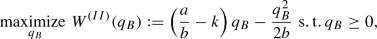 (22)
(22)then, taking the sum of the values of their optimal objectives.
- (a.1) :
-
The subproblem (21) is a concave quadratic maximization problem. By introducing the Lagrangian function \(L^{(I)}(q_A,\mu _A):=W^{(I)}(q_A)+\mu _A q_A\), it is solved through the following KKT conditions (which, for all the optimization (sub)problems studied in the paper, are necessary and sufficient for global optimalityFootnote 18, see Luenberger 1969):
$$\begin{aligned} \left\{ \begin{array}{llll} &{}{stationarity}:&{} \frac{\partial L^{(I)}}{\partial q_A}=\frac{\gamma a}{b} - k - \frac{q_A}{b} + \mu _A=0,&{}\\ &{}{primal\,feasibility}:&{} q_A \ge 0,&{}\\ &{}{dual\,feasibility}:&{} \mu _A \ge 0,&{}\\ &{}{complementary\,slackness}:&{} \mu _A q_A= 0.&{}\\ \end{array} \right. \end{aligned}$$(23)Then, it is straightforward to see that, for \(0 \le k < \frac{\gamma a}{b}\), the system (23) has \(\left( q_A=\gamma a - kb, \mu _A=0\right) \) as its unique solution, whereas, for \(k\ge \frac{\gamma a}{b}\), it has the unique solution \(\left( q_A=0, \mu _A=k-\frac{\gamma a}{b}\right) \). In the following, we denote the situation \(0 \le k < \frac{\gamma a}{b}\) by “\(l_A\)” (low marginal cost with respect to the Country A), and the situation \(k \ge \frac{\gamma a}{b}\) by “\(h_A\)” (high marginal cost with respect to the Country A). Concluding, the value of the objective function \(W^{(I)}(q_A)\) at optimality is \(\left( W^{(I)}\right) _{l_A}^\star =\frac{\left( \gamma a - kb\right) ^2}{2 b} -C_F\) in case of a low marginal cost with respect to A, and \(\left( W^{(I)}\right) _{h_A}^\star =-C_F\) in case of a high marginal cost with respect to A.
- (a.2) :
-
Similarly, also (22) is a concave quadratic maximization problem. Again, by introducing the Lagrangian function \(L^{(II)}(q_B):=W^{(II)}(q_B)+\mu _B q_B,\) it is solved through the following KKT conditions:
$$\begin{aligned} \left\{ \begin{array}{llll} &{}{stationarity}:&{} \frac{\partial L^{(II)}}{\partial q_B}=\frac{a}{b} - k - \frac{q_B}{b} + \mu _B=0,&{}\\ &{}{primal\,feasibility}:&{} q_B \ge 0,&{}\\ &{}{dual\,feasibility}:&{} \mu _B \ge 0,&{}\\ &{}{complementary\,slackness}:&{} \mu _B q_B = 0.&{}\\ \end{array} \right. \end{aligned}$$(24)Again, one can see that, for \(0 \le k < \frac{a}{b}\), the system (24) has the unique solution \(\left( q_B=a - kb, \mu _B=0\right) \) whereas, for \(k\ge \frac{a}{b}\), it has \(\left( q_B=0, \mu _B=k-\frac{a}{b}\right) \) as its unique solution. We denote the case \(0 \le k < \frac{a}{b}\) by “\(l_B\)”, and the case \(k \ge \frac{a}{b}\) by “\(h_B\)”. Then, \(\left( W^{(II)}\right) _{l_B}^\star =\frac{\left( a - kb\right) ^2}{2 b}\) and \(\left( W^{(II)}\right) _{h_B}^\star =0\). Summarizing, the optimal value of the objective function \(W(q_A,q_B)\) of the original optimization problem (20) is
$$\begin{aligned} \left( W\right) ^{RD, \star }= \left( W^{(I)}\right) ^\star +\left( W^{(II)}\right) ^\star , \end{aligned}$$(25)which has the expression
$$\begin{aligned}&\left( W\right) ^{RD, \star }=&\left\{ \begin{array}{llll} &{} W\left( \gamma a - kb, a - kb\right) -C_F=\frac{\left( \gamma a - kb\right) ^2}{2 b}+\frac{\left( a - kb\right) ^2}{2 b} -C_F, &{}\mathrm{if\,\,} 0 \le k< \frac{a}{b},&{}\\ &{} W\left( \gamma a - kb, 0 \right) -C_F=\frac{\left( \gamma a - kb\right) ^2}{2 b} -C_F, &{}\mathrm{if\,\,} \frac{a}{b} \le k < \frac{\gamma a}{b},&{}\\ &{} -C_F, &{}\mathrm{if\,\,} k \ge \frac{\gamma a}{b}.&{}\\ \end{array} \right. \nonumber \\ \end{aligned}$$(26) - (b) :
-
When the manufacturer does not invest in R&D, one has \(\left( W\right) ^{NRD, \star }=0\).
- (c) :
-
In the first decisional stage, of the two cases RD and NRD, the global planner prefers the one with the highest value of the global welfare (or it is indifferent, when they produce the same value). Then, one obtains Eq. (6), which concludes the proof. \(\square \)


Proof of Proposition 2
- (a) :
-
We first consider the case (modeling the second decisional stage) in which the manufacturer has decided to invest in R&D and incurred the total fixed cost \(C_F\). Then, any common price \(\bar{p}^{RD, \star }\) that is optimal for the manufacturer is obtained maximizing its surplus \(\varPi \), subject to \(\bar{p} \ge k\), and to one of the following constraints (whose choice depends on the value assumed by \(\bar{p}\)). These correspond, respectively, to the three subcases (2a), (2b), (2c) presented at the beginning of Sect. 5 (when the set of admissible solutions for one of these subproblems is empty, by convention we set its optimal value to \(-\infty \)):
- (a.1) :
-
if the common price \(\bar{p}\) is lower than or equal to \(\frac{a}{b}\), then the quantities \(q_A\) and \(q_B\) of the product bought by the consumers in A and B are described, respectively, by the negative-slope linear parts of the two demand functions in Eq. (1);
- (a.2) :
-
if \(\bar{p}\) is higher than or equal to \(\frac{a}{b}\), but lower than or equal to \(\frac{\gamma a}{b}\), then \(q_A\) is still described by the negative-slope linear part of the first demand function in Eq. (1), whereas \(q_B\) is equal to 0, because the market in the Country B cannot be served;
- (a.3) :
-
if \(\bar{p}\) is higher than or equal to \(\frac{\gamma a}{b}\), then both quantities \(q_A\) and \(q_B\) are equal to 0.
Although the objective function \(\varPi \) of the resulting optimization problem is concave, the “global” equality constraints on \(q_A\) and \(q_B\) that are obtained by taking into account all the three cases above, are only piecewise-linear, hence one does not obtain a concave maximization problem. However, in order to find its optimal solution and the optimal value of its objective function, one can still decompose such a problem into the three following subproblems:


which are concave maximization problems, more amenable to an analysis through standard Lagrange multipliers techniques. Indeed, their domains constitute a partition of the domain of the original optimization problem, as they correspond, respectively, to the three cases (a.1), (a.2), (a.3) above, and their objective functions coincide, in the respective domains, with the one of such optimization problem. Finally, once an optimal common price has been found for each of the three subproblems (27), (28), and (29), one chooses, among such prices, the one that corresponds to the maximum among the optimal values of their three objective functions, thus solving the original optimization problem. We now address in more detail the three subproblems (27), (28), and (29).
- (a.1):
-
The subproblem (27), which is feasible for \(0 \le k \le \frac{a}{b}\), is solved by introducing the following Lagrangian function
$$\begin{aligned} L_{UPS}^{(I)}(\bar{p},\bar{\mu },\mu _{A},\mu _{B}):=(\bar{p} -k) \left( (\gamma +1) a - 2 b \bar{p}\right) -C_F + \bar{\mu }(\bar{p}-k) + \mu _A(\gamma a - b \bar{p}) + \mu _B (a - b \bar{p}),\nonumber \\ \end{aligned}$$(30)and imposing the following KKT conditions:
$$\begin{aligned} \left\{ \begin{array}{ll} {stationarity}: &{}\quad \frac{\partial L_{UPS}^{(I)}}{\partial \bar{p}}=(\gamma +1)a - 4b\bar{p}+2kb + \bar{\mu }-\mu _A b - \mu _B b=0,\\ {primal\,feasibility}: &{}\quad \gamma a - b \bar{p} \ge 0, a - b \bar{p} \ge 0, \bar{p} \ge k,\\ {dual\,feasibility}: &{}\quad \bar{\mu }, \mu _A, \mu _B \ge 0,\\ {complementary\,slackness}:&{}\quad \bar{\mu }(\bar{p}-k), \mu _A (\gamma a - b \bar{p}), \mu _B (a - b \bar{p})= 0.\\ \end{array} \right. \end{aligned}$$(31)Then, by solving the system (31), one gets that its optimal solution \(\bar{p}^{(I), \star }\), the corresponding optimal value \(\varPi ^{(I),\star }\) of its objective function, and the corresponding optimal quantities \(q_A^{(I), \star }\) and \(q_B^{(I), \star }\), have the following expressions, depending on the values of \(\gamma \) and k:
$$\begin{aligned} \,\,\,\,\,\,\,\,\,\,\,\,\mathrm{if\,\,} 0 \le k \le \frac{a}{b} {\,\,\mathrm and\,\,} 1< \gamma < 3-\frac{2 k b}{a}: \left\{ \begin{array}{ll} &{}\bar{p}^{(I), \star }=\frac{(\gamma +1)a}{4b}+\frac{k}{2},\\ &{}\varPi ^{(I),\star }=\frac{b}{8}\left( \frac{(\gamma +1)a}{b}-2k\right) ^2-C_F,\\ &{}q_A^{(I), \star }=\gamma a -b \left( \frac{(\gamma +1)a}{4b}+\frac{k}{2}\right)>0,\\ &{}q_B^{(I), \star }=a -b \left( \frac{(\gamma +1)a}{4b}+\frac{k}{2}\right) >0,\\ \end{array} \right. \end{aligned}$$(32)$$\begin{aligned} \left. \,\,\,\,\,\,\,\,\,\,\,\,\mathrm{if\,\,} 0 \le k \le \frac{a}{b},\,\, \gamma> 1, {\,\,\mathrm and\,\,} \gamma \ge 3-\frac{2 k b}{a}: \left\{ \begin{array}{ll} &{}\bar{p}^{(I), \star }=\frac{a}{b},\,\,\,\,\,\,\,\,\,\,\,\,\,\,\,\,\,\,\,\,\,\,\,\,\,\,\,\,\,\,\,\,\,\,\\ &{}\varPi ^{(I),\star }=a (\gamma -1) \left( \frac{a}{b}-k\right) -C_F,\\ &{}q_A^{(I), \star }=(\gamma -1) a>0,\,\,\,\,\,\,\,\,\,\,\,\,\,\,\,\,\,\,\,\,\,\,\,\,\,\,\,\,\,\,\,\,\,\,\\ &{}q_B^{(I), \star }=0.\,\,\,\,\,\,\,\,\,\,\,\,\,\,\,\,\,\,\,\,\,\,\,\,\,\,\,\,\,\,\,\,\,\,\\ \end{array} \right. \right. \end{aligned}$$(33) - (a.2):
-
The subproblem (28), which is feasible for \(0 \le k \le \frac{\gamma a}{b}\), is solved by a similar Lagrange multipliers technique, providing the following expressions, depending on the values of \(\gamma \) and k:
$$\begin{aligned}&\mathrm{if\,\,} 0 \le k< \frac{a}{b} {\,\,\mathrm and\,\,} 1 < \gamma \le 2-\frac{k b}{a}: \left\{ \begin{array}{ll} &{}\bar{p}^{(II), \star }=\frac{a}{b},\\ &{}\varPi ^{(II),\star }=a (\gamma -1) \left( \frac{a}{b}-k\right) -C_F,\\ &{}q_A^{(II), \star }=(\gamma -1)a >0,\\ &{}q_B^{(II), \star }=0,\\ \end{array} \right. \end{aligned}$$(34)$$\begin{aligned}&\mathrm{if\,\,} 0 \le k< \frac{a}{b} {\,\,\mathrm and\,\,} \gamma> 2-\frac{k b}{a} \mathrm{\,\,or \,\,} \frac{a}{b} \le k < \frac{\gamma a}{b}:\, \left\{ \begin{array}{ll} &{}\bar{p}^{(II), \star }=\frac{\gamma a}{2b} + \frac{k}{2},\,\,\,\,\,\,\,\,\,\,\,\,\,\,\,\,\,\,\,\,\,\,\,\,\,\,\,\,\,\,\,\,\,\,\\ &{}\varPi ^{(II),\star }=\frac{b}{4}\left( \frac{\gamma a}{b}-k\right) ^2-C_F,\\ &{}q_A^{(II), \star }=\frac{\gamma a}{2}-\frac{kb}{2}>0,\,\,\,\,\,\,\,\,\,\,\,\,\,\,\,\,\,\,\,\,\,\,\,\,\,\,\,\,\,\,\,\,\,\,\\ &{}q_B^{(II), \star }=0,\,\,\,\,\,\,\,\,\,\,\,\,\,\,\,\,\,\,\,\,\,\,\,\,\,\,\,\,\,\,\,\,\,\,\\ \end{array} \right. \end{aligned}$$(35)$$\begin{aligned}&\mathrm{if\,\,} k = \frac{\gamma a}{b}: \left\{ \begin{array}{ll} &{}\bar{p}^{(II), \star }=\frac{\gamma a}{b},\\ &{}\varPi ^{(II),\star }= -C_F,\\ &{}q_A^{(II), \star }=0,\\ &{}q_B^{(II), \star }=0.\\ \end{array} \right. \end{aligned}$$(36) - (a.3):
-
Finally, the subproblem (29), which is feasible for \(0 \le k < + \infty \), is solved trivially by any of its feasible solutions, providing
$$\begin{aligned} \,\,\,\,\,\,\,\,\,\,\,\,\,\,\,\,\left\{ \begin{array}{ll} &{}\bar{p}^{(III), \star }= \mathrm{\,\,any\,\,} \bar{p} \ge \max \left\{ \frac{\gamma a}{b},k\right\} ,\\ &{}\varPi ^{(III),\star }=-C_F,\\ &{}q_A^{(III), \star }=0,\\ &{}q_B^{(III), \star }=0.\\ \end{array} \right. \end{aligned}$$(37)
To conclude the analysis of the second decisional stage, one sets
and takes \(\bar{p}^{RD, \star }\) to be equal to the optimal common price from (32)–(37) that corresponds to \(\varPi ^{RD, \star }\) (in case of multiple such prices, we select one associated with the lowest global welfare value).
The following notes are useful to detect, under each condition, which of the three subproblems provides \(\varPi ^{RD, \star }\) as its optimal manufacturer’s surplus, hence to determine \(\varPi ^{RD, \star }\) itself. Indeed, a comparison of Eqs. (32)–(37) shows that:
-
1.
for \(0 \le k < \frac{a}{b}\) and \(1 < \gamma \le 2-\frac{k b}{a}\), one has (noticing that the condition \(2-\frac{kb}{a} < 3-\frac{2 k b}{a}\) holds)
$$\begin{aligned} \frac{b}{8}\left( \frac{(\gamma +1)a}{b}-2k\right) ^2-C_F \ge a(\gamma -1)\left( \frac{a}{b}-k\right) -C_F \ge - C_F, \end{aligned}$$(39)since both the optimal common prices \(\bar{p}^{(I), \star }\) and \(\bar{p}^{(II), \star }\) from Eqs. (32) and (34), respectively, are feasible for the subproblem (27). Moreover, the first equality in Eq. (39) holds if and only if the two prices above coincide, since the objective function of the subproblem (27) is strictly concave;
-
2.
for \(0 \le k < \frac{a}{b}\) and \(2-\frac{k b}{a}<\gamma < 1+\sqrt{2}\left( 1-\frac{kb}{a}\right) \) (which is less than \(3-\frac{2 k b}{a}\)), one has
$$\begin{aligned} \frac{b}{8}\left( \frac{(\gamma +1)a}{b}-2k\right) ^2 - C_F > \frac{b}{4}\left( \frac{\gamma a}{b}-k\right) ^2-C_F \ge - C_F, \end{aligned}$$(40)which one can re-write, after some algebraic steps, as the quadratic inequality \(\gamma ^2 - 2 \gamma - 1 - 2 \left( \frac{kb}{a}\right) ^2 + \frac{4 kb}{a} < 0\), whose solution provides the threshold \(1+\sqrt{2}\left( 1-\frac{kb}{a}\right) \) in Eqs. (7) and (9) in the statement of Proposition 2. Similarly, the first inequality in (40) holds with “>” replaced by “<” for \(1+\sqrt{2}\left( 1-\frac{kb}{a}\right)< \gamma < 3-\frac{2 kb}{a}\), and by “\(=\)” for \(\gamma =1+\sqrt{2}\left( 1-\frac{kb}{a}\right) \);
-
3.
for \(0 \le k < \frac{a}{b}\) and \(\gamma \ge 3-\frac{2 k b}{a}\), one gets
$$\begin{aligned} \frac{b}{4}\left( \frac{\gamma a}{b}-k\right) ^2-C_F \ge a(\gamma -1)\left( \frac{a}{b}-k\right) -C_F \ge -C_F, \end{aligned}$$(41)since both the optimal common prices \(\bar{p}^{(I), \star }\) and \(\bar{p}^{(II), \star }\) from (33) and (35), respectively, are feasible for the subproblem (28). Again, the first equality in (41) holds if and only if the two prices above coincide.
(b) The optimization problem in the first decisional stage is solved using the expression (38) of \(\varPi ^{RD, \star }\) and Eqs. (39)–(41). From these, one gets Eqs. (7) and (8) (this completes the proof of item (i)), then Eqs. (9) and (10) (this completes the proof of item (ii)). Item (iii) is obtained straightforwardly, and has been reported only for the completeness of the analysis. \(\square \)
Proof of Proposition 3
The main difference with respect to the proof of Proposition 2 is that the subproblems (27)–(29) of its second decisional stage are now replaced by the following subproblems, which are solved by using similar techniques:


We report only the results related to to the first two subproblems, since the third one is trivial:
From these expressions, one obtains Eqs. (11)–(14), in a similar way as in the proof of Proposition 2. \(\square \)
Proof of Proposition 4
- (a) :
-
The main difference with respect to the proof of Proposition 2 is that the subproblems (27)–(29) of its second decisional stage are now replaced by
 (47)
(47)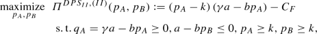 (48)
(48)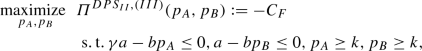 (49)
(49)where we have taken into account that the constraint \(\left| p_A-p_B\right| \le t\) is needed only when both \(q_A\) and \(q_B\) are positive, i.e., only in the optimization subproblem (47). In the following, we report only the results of the first two subproblems, being the third one trivial.
- (a.1) :
-
The optimization subproblem (47) is feasible for \(0 \le k < \frac{a}{b}\). For such a case, its optimal solution \(p_A^{DPS_{II},(I),\star }\), \(p_B^{DPS_{II},(I),\star }\), the corresponding optimal value \(\varPi ^{DPS_{II},(I),\star }\) of its objective function, and the corresponding optimal quantities \(q_A^{DPS_{II},(I),\star }\) and \(q_B^{DPS_{II},(I),\star }\), are determined in the following way.


For \(0 \le k < \frac{a}{b}\) and \(t \ge \frac{(\gamma -1)a}{2b}\), the unconstrained maximizer of the strictly concave function \(\varPi ^{DPS_{II},(I),\star }\) (which is \(p_A=\frac{\gamma a}{b}+\frac{k}{2}\), \(p_B=\frac{a}{b}+\frac{k}{2}\)) is feasible also for the optimization subproblem (47). Hence, it is also its optimal solution, and one gets the following:
For \(0 \le k < \frac{a}{b}\) and \(0< t < \frac{(\gamma -1)a}{2b}\), instead, the unconstrained maximizer of the strictly concave function \(\varPi ^{DPS_{II},(I),\star }\) is not feasible for the optimization subproblem (47). Moreover, one can observe that, at optimality for such optimization subproblem, one has always \(p_A \ge p_B\) (otherwise, the manufacturer could switch the two prices, obtaining a higher profit). Further, one can also notice that there exists no optimal solution with \(p_A=\frac{\gamma a}{b}\) (because, in that case, the constraints \(p_B \ge p_A-t\), \(p_B < \frac{a}{b}\) and \(0< t < \frac{(\gamma -1)a}{2b}\) are incompatible) and also with \(p_B=k\) and \(k<p_A<k+t\) (because the unconstrained maximizer \(p_A=\frac{\gamma a}{2b}+\frac{k}{2}\) does not satisfy the constraint \(p_A<k+t\)). Then, the optimal solution to the optimization subproblem (47) has to be searched inside the following set of candidate optimal solutions:
-
1.
\(p_A=p_B=k\) (for which one has \(\varPi ^{DPS_{II},(I)}=-C_F\));
-
2.
the optimal solution to the following optimization subproblem (which corresponds to a difference in prices equal to t):
 (51)
(51)Such an optimal solution exists for \(\gamma < 3+\frac{2b}{a}(t-k)\), and in that case is \(p_A=\frac{(\gamma +1)a}{4b}+\frac{k+t}{2}\) (\(p_B=\frac{(\gamma +1)a}{4b}+\frac{k-t}{2}\)), and is associated with
$$\begin{aligned} \varPi ^{DPS_{II},(I)}= & {} \left( \frac{(\gamma +1)a}{4b}+\frac{k+t}{2}-k\right) \left( \gamma a-b \left( \frac{(\gamma +1)a}{4b}+\frac{k+t}{2}\right) \right) \nonumber \\&+\left( \frac{(\gamma +1)a}{4b}+\frac{k-t}{2}-k\right) \left( a-b \left( \frac{(\gamma +1)a}{4b}+\frac{k-t}{2}\right) \right) -C_F \nonumber \\> & {} -C_F. \end{aligned}$$(52)

Concluding, comparing the two cases above, one obtains the following optimal solution for the subproblem (47):
Finally, if \(0 \le k < \frac{a}{b}\), \(0< t < \frac{(\gamma -1)a}{2b}\), and \(\gamma \ge 3+\frac{2b}{a}(t-k)\), then there exists no optimal solution to the subproblem (47) (because \(p_A=\frac{(\gamma +1)a}{4b}+\frac{k+t}{2}\) becomes unfeasible), and the supremum of its objective is obtained in the limiting case \(p_A \rightarrow \frac{a}{b}+t\), which is associated with \(\varPi ^{DPS_{II},(I)}=\left( \frac{a}{b}+t-k\right) \left( \gamma a -a -b t + kb\right) -C_F>-C_F\) (this limiting case is taken into account in the optimization subproblem (48), as it is feasible for it).
- (a.2):
-
The optimization subproblem (48) is feasible for \(0 \le k \le \frac{\gamma a}{b}\). For such a subproblem, applying a similar Lagrange multipliers technique, one obtains:
$$\begin{aligned} \mathrm{if}\; 0 \le k \le \frac{\gamma a}{b} \;\mathrm{and}\; \gamma > 1 : \left\{ \begin{array}{ll} &{}p_A^{DPS_{II},(II),\star }=\frac{\gamma a}{2b} + \frac{k}{2},\\ &{}p_B^{DPS_{II},(II),\star }= \mathrm{\,\,any\,\,} p_B \ge \max \left\{ \frac{a}{b},k\right\} ,\\ &{}\varPi ^{DPS_{II},(II),\star }=\frac{b}{4}\left( \frac{\gamma a}{b}-k\right) ^2-C_F,\\ &{}q_A^{DPS_{II},(II),\star }=\frac{\gamma a}{2} - \frac{kb}{2}\ge 0,\\ &{}q_B^{DPS_{II},(II),\star }=0. \end{array} \right. \end{aligned}$$(54) - (b):
-
From the expressions (50)–(54) above, one obtains (15)–(18), in a similar way as in the proof of Proposition 2. In particular, the additional threshold \(1+ \frac{2 t b}{a} + \sqrt{2}\left( 1-\frac{kb}{a}\right) \) on \(\gamma \) is derived, e.g., when comparing the optimal manufacturer’s surpluses \(\varPi ^{DPS_{II},(I),\star }\) and \(\varPi ^{DPS_{II},(II),\star }\) for \(0 \le k < \frac{a}{b}\), \(0< t < \frac{(\gamma -1)a}{2b}\) and \(1< \gamma < 3+\frac{2b}{a}(t-k)\). Indeed, after some algebraic steps, the inequality
$$\begin{aligned}&\left( \frac{(\gamma +1)a}{4b}+\frac{k+t}{2}-k\right) \left( \gamma a-b \left( \frac{(\gamma +1)a}{4b}+\frac{k+t}{2}\right) \right) \\&\quad +\left( \frac{(\gamma +1)a}{4b}+\frac{k-t}{2}-k\right) \left( a-b \left( \frac{(\gamma +1)a}{4b}+\frac{k-t}{2}\right) \right) \\&\quad > \frac{b}{4}\left( \frac{\gamma a}{b}-k\right) ^2 \end{aligned}$$can be re-written as the quadratic inequality
$$\begin{aligned} \gamma ^2 -2\left( 1+\frac{2 t b}{a}\right) \gamma -1 -2 \left( \frac{kb}{a}\right) ^2+\frac{4 kb}{a}+4\left( \frac{t b}{a}\right) ^2+\frac{4 t b}{a}<0, \end{aligned}$$(55)whose solution provides that threshold. \(\square \)
Proof of Proposition 5
The optimization problems modeling the second decisional stage become more constrained when moving from the 1st differential pricing scheme to the 2nd differential pricing scheme, and from the 2nd differential pricing scheme to the uniform pricing scheme. As a consequence, the same order is obtained when moving to the first decisional stage, proving Eq. (19). \(\square \)
Proof of Proposition 6
Items (i) and (ii) are a direct consequence of the proofs of Propositions 2, 3, and 4 (particularly, of the expressions of the associated optimal prices and quantities obtained in the various cases). \(\square \)
Appendix B: Prices and quantities at optimality for the various models
The following corollary to Proposition 1 is obtained directly from its proof. It expresses the optimal quantities for the global planner (in this specific case, no prices are reported since they do not appear in the related optimization problem, which has been considered in Appendix A).
Corollary 1
-
(i)
In case \(GW^{\star }{>0}\), the associated optimal quantities are
$$\begin{aligned} q_A^{\star }= & {} \gamma a - kb,\;\mathrm{if}\; 0 \le k < \frac{\gamma a}{b}, \end{aligned}$$(56)$$\begin{aligned} q_B^{\star }= & {} \left\{ \begin{array}{ll} a - kb,&{}\quad \mathrm{if}\; 0 \le k< \frac{a}{b},\\ 0, &{}\quad \mathrm{if}\; \frac{a}{b} \le \gamma < \frac{\gamma a}{b}.\\ \end{array} \right. \end{aligned}$$(57) -
(ii)
In case \(GW^{\star }{=0}\), the associated optimal quantities are \(q_A^{\star }=0\) and \(q_B^{\star }=0\).
It follows from the proof of Proposition 2, which has been detailed in Appendix A, that the expressions of the optimal quantities associated with the optimal manufacturer’s surplus \(\varPi _{UPS}^{\star }\) can be easily detected from its statement given above, since they are just the two arguments of the global welfare function \(W(\cdot ,\cdot )\) at optimality: e.g., the term \(W\left( \gamma a - b \left( \frac{(\gamma +1) a}{4b}+ \frac{k}{2}\right) ,a - b \left( \frac{(\gamma +1) a}{4b}+ \frac{k}{2}\right) \right) \) in Eq. (9) indicates that, in the specific case—i.e., for \(0 \le k < \frac{a}{b}\) and \(1< \gamma < 1+\sqrt{2}\left( 1-\frac{kb}{a}\right) \)—the optimal quantities for the manufacturer under the uniform pricing scheme are \(q_A^{UPS,\star }=\gamma a - b \left( \frac{(\gamma +1) a}{4b}+ \frac{k}{2}\right) \) and \(q_B^{UPS,\star }=a - b \left( \frac{(\gamma +1) a}{4b}+ \frac{k}{2}\right) \). Moreover, starting from \(q_A^{UPS,\star }\) and \(q_B^{UPS,\star }\), the optimal common price \(\bar{p}^{UPS,\star }\) is obtained immediately by applying Eq. (1). In summary, one gets the following corollary, which provides the expressions of the optimal common price and of the optimal quantities associated with Proposition 2. The corollary shows that these can have a discontinuity point for \(\gamma =1+\sqrt{2}\left( 1-\frac{kb}{a}\right) \). It also illustrates cases for which one of the two countries is not served at optimality (i.e., when the associated optimal quantity is 0). In the following, in order to simplify the notation in the corollary, we let \(W_{UPS}^{(I),\star }:=W\left( \gamma a - b \left( \frac{(\gamma +1) a}{4b}+ \frac{k}{2}\right) ,a - b \left( \frac{(\gamma +1) a}{4b}+ \frac{k}{2}\right) \right) \) and \(W_{UPS}^{(II),\star }:=W\left( \frac{\gamma a}{2}- \frac{kb}{2},0\right) \).
Corollary 2
-
(i)
In case \(\varPi _{UPS}^{\star }{>0}\), the optimal common price \(\bar{p}^{UPS,\star }\) and the optimal quantities \(q_A^{UPS,\star }\) and \(q_B^{UPS,\star }\) associated with the uniform pricing scheme are, for \(0 \le k < \frac{a}{b}\),
$$\begin{aligned}&\bar{p}^{UPS,\star }=&\left\{ \begin{array}{lll} &{}\frac{(\gamma +1) a}{4b}+ \frac{k}{2}, &{}\\ &{} \,\,\,\,\,\,\,\,\,\,\,\,\,\,\,\,\,\,\,\,\,\,\,\mathrm{if\,\,} 1< \gamma< 1+\sqrt{2}\left( 1-\frac{kb}{a}\right) &{}\\ &{} \,\,\,\,\,\,\,\,\,\,\,\,\,\,\,\,\,\,\,\,\,\,\,\mathrm{or\,\,} \gamma = 1+\sqrt{2}\left( 1-\frac{kb}{a}\right) {\,\,\mathrm and\,\,} W_{UPS}^{(I),\star } < W_{UPS}^{(II),\star },&{}\\ &{}\mathrm{either\,\,} \frac{(\gamma +1) a}{4b}+ \frac{k}{2} \mathrm{\,\,or\,\,}\frac{\gamma a}{2b}+ \frac{k}{2}, &{}\\ &{} \,\,\,\,\,\,\,\,\,\,\,\,\,\,\,\,\,\,\,\,\,\,\,\mathrm{if\,\,} \gamma = 1+\sqrt{2}\left( 1-\frac{kb}{a}\right) {\,\,\mathrm and\,\,} W_{UPS}^{(I),\star } = W_{UPS}^{(II),\star },&{}\\ &{}\frac{\gamma a}{2b}+ \frac{k}{2}, &{}\\ &{} \,\,\,\,\,\,\,\,\,\,\,\,\,\,\,\,\,\,\,\,\,\,\,\mathrm{if\,\,} \gamma = 1+\sqrt{2}\left( 1-\frac{kb}{a}\right) {\,\,\mathrm and\,\,} W_{UPS}^{(I),\star }> W_{UPS}^{(II),\star }&{}\\ &{}\,\,\,\,\,\,\,\,\,\,\,\,\,\,\,\,\,\,\,\,\,\,\,\mathrm{or\,\,} \gamma > 1+\sqrt{2}\left( 1-\frac{kb}{a}\right) ,&{} \end{array} \right. \end{aligned}$$(58)$$\begin{aligned}&q_A^{UPS,\star }=&\left\{ \begin{array}{lll} &{}\gamma a - b \left( \frac{(\gamma +1) a}{4b}+ \frac{k}{2}\right) , &{}\\ &{} \,\,\,\,\,\,\,\,\,\,\,\,\,\,\,\,\,\,\,\,\,\,\,\mathrm{if\,\,} 1< \gamma< 1+\sqrt{2}\left( 1-\frac{kb}{a}\right) &{}\\ &{} \,\,\,\,\,\,\,\,\,\,\,\,\,\,\,\,\,\,\,\,\,\,\,\mathrm{or\,\,} \gamma = 1+\sqrt{2}\left( 1-\frac{kb}{a}\right) {\,\,\mathrm and\,\,} W_{UPS}^{(I),\star } < W_{UPS}^{(II),\star },&{}\\ &{}\mathrm{either\,\,} \gamma a - b \left( \frac{(\gamma +1) a}{4b}+ \frac{k}{2}\right) \mathrm{\,\,or\,\,}\frac{\gamma a}{2}- \frac{kb}{2}, &{}\\ &{} \,\,\,\,\,\,\,\,\,\,\,\,\,\,\,\,\,\,\,\,\,\,\,\mathrm{if\,\,} \gamma = 1+\sqrt{2}\left( 1-\frac{kb}{a}\right) {\,\,\mathrm and\,\,} W_{UPS}^{(I),\star } = W_{UPS}^{(II),\star },&{}\\ &{}\frac{\gamma a}{2}- \frac{kb}{2}, &{}\\ &{} \,\,\,\,\,\,\,\,\,\,\,\,\,\,\,\,\,\,\,\,\,\,\,\mathrm{if\,\,} \gamma = 1+\sqrt{2}\left( 1-\frac{kb}{a}\right) {\,\,\mathrm and\,\,} W_{UPS}^{(I),\star }> W_{UPS}^{(II),\star }&{}\\ &{}\,\,\,\,\,\,\,\,\,\,\,\,\,\,\,\,\,\,\,\,\,\,\,\mathrm{or\,\,} \gamma > 1+\sqrt{2}\left( 1-\frac{kb}{a}\right) ,&{} \end{array} \right. \end{aligned}$$(59)$$\begin{aligned}&q_B^{UPS,\star }=&\left\{ \begin{array}{lll} &{}a - b \left( \frac{(\gamma +1) a}{4b}+ \frac{k}{2}\right) , &{}\\ &{} \,\,\,\,\,\,\,\,\,\,\,\,\,\,\,\,\,\,\,\,\,\,\,\mathrm{if\,\,} 1< \gamma< 1+\sqrt{2}\left( 1-\frac{kb}{a}\right) &{}\\ &{} \,\,\,\,\,\,\,\,\,\,\,\,\,\,\,\,\,\,\,\,\,\,\,\mathrm{or\,\,} \gamma = 1+\sqrt{2}\left( 1-\frac{kb}{a}\right) {\,\,\mathrm and\,\,} W_{UPS}^{(I),\star } < W_{UPS}^{(II),\star },&{}\\ &{}\mathrm{either\,\,} a - b \left( \frac{(\gamma +1) a}{4b}+ \frac{k}{2}\right) \mathrm{\,\,or\,\,}0, &{}\\ &{} \,\,\,\,\,\,\,\,\,\,\,\,\,\,\,\,\,\,\,\,\,\,\,\mathrm{if\,\,} \gamma = 1+\sqrt{2}\left( 1-\frac{kb}{a}\right) {\,\,\mathrm and\,\,} W_{UPS}^{(I),\star } = W_{UPS}^{(II),\star },&{}\\ &{}0, &{}\\ &{} \,\,\,\,\,\,\,\,\,\,\,\,\,\,\,\,\,\,\,\,\,\,\,\mathrm{if\,\,} \gamma = 1+\sqrt{2}\left( 1-\frac{kb}{a}\right) {\,\,\mathrm and\,\,} W_{UPS}^{(I),\star }> W_{UPS}^{(II),\star }&{}\\ &{}\,\,\,\,\,\,\,\,\,\,\,\,\,\,\,\,\,\,\,\,\,\,\,\mathrm{or\,\,} \gamma > 1+\sqrt{2}\left( 1-\frac{kb}{a}\right) ,&{} \end{array} \right. \nonumber \\ \end{aligned}$$(60)and, for \(k \ge \frac{a}{b}\) and \(\gamma > \frac{k b}{a}\),
$$\begin{aligned} \bar{p}^{UPS,\star } = \frac{\gamma a}{2b}+ \frac{k}{2}, \quad q_{A}^{UPS,\star } = \frac{\gamma a}{2}-\frac{kb}{2}, \quad q_{B}^{UPS,\star } = 0. \end{aligned}$$(61) -
(ii)
In case \(\varPi _{UPS}^{\star }{=0}\), the associated optimal common price is \(\bar{p}^{UPS, \star }=\mathrm{any\,\,} \bar{p} \ge \max \left\{ \frac{\gamma a}{b},k\right\} \), whereas the associated optimal quantities are \(q_{A}^{UPS, \star }=0\) and \(q_{B}^{UPS, \star }=0\).
In a similar way as for the uniform pricing scheme, we get the following corollary to Proposition 3, about the optimal prices and quantities for the 1st differential pricing scheme.
Corollary 3
-
(i)
In case \(\varPi _{DPS_I}^{\star }{>0}\), the optimal prices \(p_{A}^{DPS_I,\star }\) and \(p_{B}^{DPS_I,\star }\) and the optimal quantities \(q_A^{DPS_I,\star }\) and \(q_B^{DPS_I,\star }\) associated with the 1st differential pricing scheme are, for \(0 \le k < \frac{a}{b}\),
$$\begin{aligned} p_{A}^{DPS_I,\star }= & {} \frac{\gamma a}{2b}+ \frac{k}{2},\quad p_{B}^{DPS_I,\star } =\frac{a}{2b}+ \frac{k}{2} , \end{aligned}$$(62)$$\begin{aligned} q_{A}^{DPS_I,\star }= & {} \frac{\gamma a}{2}- \frac{kb}{2},\quad q_{B}^{DPS_I,\star } =\frac{a}{2}- \frac{kb}{2}, \end{aligned}$$(63)and, for \(k \ge \frac{a}{b}\) and \(\gamma > \frac{k b}{a}\),
$$\begin{aligned} p_{A}^{DPS_I,\star }= & {} \frac{\gamma a}{2b}+ \frac{k}{2}, \quad p_{B}^{DPS_I,\star } = \mathrm{any\,\,} p_B \ge \max \left\{ \frac{a}{b},k\right\} , \end{aligned}$$(64)$$\begin{aligned} q_{A}^{DPS_I,\star }= & {} \frac{\gamma a}{2}- \frac{kb}{2}, \quad q_{B}^{DPS_I,\star } = 0. \end{aligned}$$(65) -
(ii)
In case \(\varPi _{DPS_I}^{\star }{=0}\), the associated optimal prices are \(p_{A}^{DPS_I, \star }=\mathrm{any\,\,} p_A \ge \max \left\{ \frac{\gamma a}{b},k\right\} \) and \(p_{B}^{DPS_I, \star }=\mathrm{any\,\,} p_B \ge \max \left\{ \frac{a}{b},k\right\} \), whereas the associated optimal quantities are \(q_{A}^{DPS_I, \star }=0\) and \(q_{B}^{DPS_I, \star }=0\).
Finally, in a similar way as for the uniform pricing scheme and for the 1st differential pricing scheme, we get the following corollary to Proposition 4 about the optimal prices and quantities for the 2nd differential pricing scheme. The corollary shows that these can have a discontinuity point for \(\gamma =1+\frac{2 t b}{a} + \sqrt{2} \left( 1-\frac{kb}{a}\right) \). In the following, in order to simplify the notation in the corollary, we let \(W_{DPS_{II}}^{(I),\star }:=W\left( \gamma a - b \left( \frac{(\gamma +1) a}{4b}+ \frac{k+t}{2}\right) ,a - b \left( \frac{(\gamma +1) a}{4b}+ \frac{k-t}{2}\right) \right) \) and \(W_{DPS_{II}}^{(II),\star }:=W\left( \frac{\gamma a}{2}- \frac{kb}{2},0\right) \).
Corollary 4
-
(i)
In case \(\varPi _{DPS_{II}}^{\star }{>0}\), the optimal prices \(p_{A}^{DPS_{II},\star }\) and \(p_{B}^{DPS_{II},\star }\) and the optimal quantities \(q_A^{DPS_{II},\star }\) and \(q_B^{DPS_{II},\star }\) associated with the 2nd differential pricing scheme are, for \(0 \le k < \frac{a}{b}\),
$$\begin{aligned}&p_{A}^{DPS_{II},\star }=&\left\{ \begin{array}{lll} &{}\frac{\gamma a}{2b}+\frac{k}{2},\,\,\,\,\mathrm{if\,\,} 1< \gamma \le 1+\frac{2 t b}{a},&{}\\ &{}\frac{(\gamma +1)a}{4 b}+ \frac{k+t}{2}, \,\,\,\,\,\,\,\,\,\,\,\,\,\,\,\,\,\,\,\,&{}\\ &{}\,\,\,\,\,\,\,\,\,\,\,\,\,\,\,\,\,\,\,\,\,\,\,\,\,\,\,\mathrm{if\,\,} 1+\frac{2 t b}{a}< \gamma< 1+\frac{2 t b}{a} + \sqrt{2} \left( 1-\frac{kb}{a}\right) &{}\\ &{}\,\,\,\,\,\,\,\,\,\,\,\,\,\,\,\,\,\,\,\,\,\,\,\,\,\,\,\mathrm{or\,\,} \gamma = 1+\frac{2 t b}{a} + \sqrt{2} \left( 1-\frac{kb}{a}\right) {\,\,\mathrm and \,\,} W_{DPS_{II}}^{(I),\star } < W_{DPS_{II}}^{(II),\star },&{}\\ &{}\mathrm{either\,\,} \frac{(\gamma +1)a}{4 b}+ \frac{k+t}{2} {\,\,\mathrm or \,\,} \frac{\gamma a}{2b}+ \frac{k}{2},&{} \\ &{}\,\,\,\,\,\,\,\,\,\,\,\,\,\,\,\,\,\,\,\,\,\,\,\,\,\,\,\mathrm{if\,\,} \gamma = 1+\frac{2 t b}{a} + \sqrt{2} \left( 1-\frac{kb}{a}\right) {\,\,\mathrm and \,\,} W_{DPS_{II}}^{(I),\star } = W_{DPS_{II}}^{(II),\star },&{}\\ &{}\frac{\gamma a}{2b}+ \frac{k}{2},&{}\\ &{}\,\,\,\,\,\,\,\,\,\,\,\,\,\,\,\,\,\,\,\,\,\,\,\,\,\,\,\mathrm{if\,\,} \gamma = 1+\frac{2 t b}{a} + \sqrt{2} \left( 1-\frac{kb}{a}\right) {\,\,\mathrm and \,\,} W_{DPS_{II}}^{(I),\star }> W_{DPS_{II}}^{(II),\star }&{}\\ &{}\,\,\,\,\,\,\,\,\,\,\,\,\,\,\,\,\,\,\,\,\,\,\,\,\,\,\,\mathrm{or\,\,} \gamma > 1+\frac{2 t b}{a} + \sqrt{2} \left( 1-\frac{kb}{a}\right) ,&{} \end{array} \right. \end{aligned}$$(66)$$\begin{aligned}&p_{B}^{DPS_{II},\star }=&\left\{ \begin{array}{lll} &{}\frac{a}{2b}+\frac{k}{2},\,\,\,\,\mathrm{if\,\,} 1< \gamma \le 1+\frac{2 t b}{a},&{}\\ &{}\frac{(\gamma +1)a}{4 b}+ \frac{k-t}{2}, \,\,\,\,\,\,\,\,\,\,\,\,\,\,\,\,\,\,\,\,&{}\\ &{}\,\,\,\,\,\,\,\,\,\,\,\,\,\,\,\,\,\,\,\,\,\,\,\,\,\,\,\mathrm{if\,\,} 1+\frac{2 t b}{a}< \gamma< 1+\frac{2 t b}{a} + \sqrt{2} \left( 1-\frac{kb}{a}\right) &{}\\ &{}\,\,\,\,\,\,\,\,\,\,\,\,\,\,\,\,\,\,\,\,\,\,\,\,\,\,\,\mathrm{or\,\,} \gamma = 1+\frac{2 t b}{a} + \sqrt{2} \left( 1-\frac{kb}{a}\right) {\,\,\mathrm and \,\,} W_{DPS_{II}}^{(I),\star } < W_{DPS_{II}}^{(II),\star },&{}\\ &{}\mathrm{either\,\,} \frac{(\gamma +1)a}{4 b}+ \frac{k+t}{2} {\,\,\mathrm or \,\,} \mathrm{any\,\,} p_B \ge \max \left\{ \frac{a}{b},k\right\} ,&{} \\ &{}\,\,\,\,\,\,\,\,\,\,\,\,\,\,\,\,\,\,\,\,\,\,\,\,\,\,\,\mathrm{if\,\,} \gamma = 1+\frac{2 t b}{a} + \sqrt{2} \left( 1-\frac{kb}{a}\right) {\,\,\mathrm and \,\,} W_{DPS_{II}}^{(I),\star } = W_{DPS_{II}}^{(II),\star },&{}\\ &{}\mathrm{any\,\,} p_B \ge \max \left\{ \frac{a}{b},k\right\} ,&{}\\ &{}\,\,\,\,\,\,\,\,\,\,\,\,\,\,\,\,\,\,\,\,\,\,\,\,\,\,\,\mathrm{if\,\,} \gamma = 1+\frac{2 t b}{a} + \sqrt{2} \left( 1-\frac{kb}{a}\right) {\,\,\mathrm and \,\,} W_{DPS_{II}}^{(I),\star }> W_{DPS_{II}}^{(II),\star }&{}\\ &{}\,\,\,\,\,\,\,\,\,\,\,\,\,\,\,\,\,\,\,\,\,\,\,\,\,\,\,\mathrm{or\,\,} \gamma > 1+\frac{2 t b}{a} + \sqrt{2} \left( 1-\frac{kb}{a}\right) ,&{} \end{array} \right. \end{aligned}$$(67)$$\begin{aligned}&q_{A}^{DPS_{II},\star }=&\left\{ \begin{array}{lll} &{}\frac{\gamma a}{2}-\frac{kb}{2},\,\,\,\,\mathrm{if\,\,} 1< \gamma \le 1+\frac{2 t b}{a},&{}\\ &{}\gamma a -b \left( \frac{(\gamma +1)a}{4 b}+ \frac{k+t}{2}\right) , \,\,\,\,\,\,\,\,\,\,\,\,\,\,\,\,\,\,\,\,&{}\\ &{}\,\,\,\,\,\,\,\,\,\,\,\,\,\,\,\,\,\,\,\,\,\,\,\,\,\,\,\mathrm{if\,\,} 1+\frac{2 t b}{a}< \gamma< 1+\frac{2 t b}{a} + \sqrt{2} \left( 1-\frac{kb}{a}\right) &{}\\ &{}\,\,\,\,\,\,\,\,\,\,\,\,\,\,\,\,\,\,\,\,\,\,\,\,\,\,\,\mathrm{or\,\,} \gamma = 1+\frac{2 t b}{a} + \sqrt{2} \left( 1-\frac{kb}{a}\right) {\,\,\mathrm and \,\,} W_{DPS_{II}}^{(I),\star } < W_{DPS_{II}}^{(II),\star },&{}\\ &{}\mathrm{either\,\,} \gamma a -b \left( \frac{(\gamma +1)a}{4 b}+ \frac{k+t}{2}\right) {\,\,\mathrm or \,\,} \frac{\gamma a}{2}- \frac{kb}{2},&{} \\ &{}\,\,\,\,\,\,\,\,\,\,\,\,\,\,\,\,\,\,\,\,\,\,\,\,\,\,\,\mathrm{if\,\,} \gamma = 1+\frac{2 t b}{a} + \sqrt{2} \left( 1-\frac{kb}{a}\right) {\,\,\mathrm and \,\,} W_{DPS_{II}}^{(I),\star } = W_{DPS_{II}}^{(II),\star },&{}\\ &{}\frac{\gamma a}{2}- \frac{kb}{2},&{}\\ &{}\,\,\,\,\,\,\,\,\,\,\,\,\,\,\,\,\,\,\,\,\,\,\,\,\,\,\,\mathrm{if\,\,} \gamma = 1+\frac{2 t b}{a} + \sqrt{2} \left( 1-\frac{kb}{a}\right) {\,\,\mathrm and \,\,} W_{DPS_{II}}^{(I),\star }> W_{DPS_{II}}^{(II),\star }&{}\\ &{}\,\,\,\,\,\,\,\,\,\,\,\,\,\,\,\,\,\,\,\,\,\,\,\,\,\,\,\mathrm{or\,\,} \gamma > 1+\frac{2 t b}{a} + \sqrt{2} \left( 1-\frac{kb}{a}\right) ,&{} \end{array} \right. \end{aligned}$$(68)$$\begin{aligned}&q_{B}^{DPS_{II},\star }=&\left\{ \begin{array}{lll} &{}\frac{a}{2}-\frac{kb}{2},\,\,\,\,\mathrm{if\,\,} 1< \gamma \le 1+\frac{2 t b}{a},&{}\\ &{}a -b \left( \frac{(\gamma +1)a}{4 b}+ \frac{k-t}{2}\right) , \,\,\,\,\,\,\,\,\,\,\,\,\,\,\,\,\,\,\,\,&{}\\ &{}\,\,\,\,\,\,\,\,\,\,\,\,\,\,\,\,\,\,\,\,\,\,\,\,\,\,\,\mathrm{if\,\,} 1+\frac{2 t b}{a}< \gamma< 1+\frac{2 t b}{a} + \sqrt{2} \left( 1-\frac{kb}{a}\right) &{}\\ &{}\,\,\,\,\,\,\,\,\,\,\,\,\,\,\,\,\,\,\,\,\,\,\,\,\,\,\,\mathrm{or\,\,} \gamma = 1+\frac{2 t b}{a} + \sqrt{2} \left( 1-\frac{kb}{a}\right) {\,\,\mathrm and \,\,} W_{DPS_{II}}^{(I),\star } < W_{DPS_{II}}^{(II),\star },&{}\\ &{}\mathrm{either\,\,} a -b \left( \frac{(\gamma +1)a}{4 b}+ \frac{k-t}{2}\right) {\,\,\mathrm or \,\,} 0,&{} \\ &{}\,\,\,\,\,\,\,\,\,\,\,\,\,\,\,\,\,\,\,\,\,\,\,\,\,\,\,\mathrm{if\,\,} \gamma = 1+\frac{2 t b}{a} + \sqrt{2} \left( 1-\frac{kb}{a}\right) {\,\,\mathrm and \,\,} W_{DPS_{II}}^{(I),\star } = W_{DPS_{II}}^{(II),\star },&{}\\ &{}0,&{}\\ &{}\,\,\,\,\,\,\,\,\,\,\,\,\,\,\,\,\,\,\,\,\,\,\,\,\,\,\,\mathrm{if\,\,} \gamma = 1+\frac{2 t b}{a} + \sqrt{2} \left( 1-\frac{kb}{a}\right) {\,\,\mathrm and \,\,} W_{DPS_{II}}^{(I),\star }> W_{DPS_{II}}^{(II),\star }&{}\\ &{}\,\,\,\,\,\,\,\,\,\,\,\,\,\,\,\,\,\,\,\,\,\,\,\,\,\,\,\mathrm{or\,\,} \gamma > 1+\frac{2 t b}{a} + \sqrt{2} \left( 1-\frac{kb}{a}\right) ,&{} \end{array} \right. \end{aligned}$$(69)and, for \(k \ge \frac{a}{b}\) and \(\gamma > \frac{k b}{a}\),
$$\begin{aligned}&p_A^{DPS_{II},\star } = \frac{\gamma a}{2b}+ \frac{k}{2}, \,\,\,\, p_B^{DPS_{II},\star } = \mathrm{any\,\,} p_B \ge \max \left\{ \frac{a}{b},k\right\} , \end{aligned}$$(70)$$\begin{aligned}&q_A^{DPS_{II},\star } = \frac{\gamma a}{2}- \frac{kb}{2}, \,\,\,\, q_B^{DPS_{II},\star } = 0. \end{aligned}$$(71) -
(ii)
In case \(\varPi _{DPS_{II}}^{\star }{=0}\), the associated optimal prices are \(p_{A}^{DPS_{II}, \star }=\mathrm{any\,\,} p_A \ge \max \left\{ \frac{\gamma a}{b},k\right\} \) and \(p_{B}^{DPS_{II}, \star }=\mathrm{any\,\,} p_B \ge \max \left\{ \frac{a}{b},k\right\} \), whereas the associated optimal quantities are \(q_{A}^{DPS_{II}, \star }=0\) and \(q_{B}^{DPS_{II}, \star }=0\).
Appendix C: Some technical remarks about the various models considered
In the following, some technical remarks are reported regarding the models considered in Sects. 5.1, 5.2, 5.3. In particular, some common aspects of these models are highlighted.
Remark 1
Optimal prices and quantities for the uniform pricing scheme and for each of the two differential pricing schemes have been reported in Appendix B, as functions of \(\gamma \) (see Corollaries 2, 3, and 4). In particular, Corollaries 2 and 4 show the presence of a discontinuity point in these functions. Moreover, Corollaries 2 and 4 show that, for the corresponding model, the values of the optimal price(s) and quantities at the discontinuity point can be obtained simply by finding, in a first step, the maximum between the left and right limit of the global welfare at the discontinuity point, then, in a second step, taking the associated limiting price(s) and quantities: e.g., making \(\gamma \) tend to the discontinuity point from the left (respectively, from the right) in the second step if the maximum in the first step is obtained in correspondence of the left limit (respectively, right limit).
Remark 2
Corollaries 2, and 3, and 4 show that, for \(k \ge \frac{a}{b}\), all the pricing schemes are equivalent at optimality (i.e., they are associated with the same optimal prices and quantities), since the Country B is never served in that case. Moreover, Corollary 4 and its comparison with Corollaries 2 and 3 show that, for \(0 \le k < \frac{a}{b}\) and fixed \(t>0\), at optimality, the 2nd differential pricing scheme is a “ hybrid” between the uniform pricing scheme and the 1st differential pricing scheme, in the following sense:
-
1.
in the range \(1 < \gamma \le 1+\frac{2tb}{a}\), it is equivalent to the 1st differential pricing scheme;
-
2.
in the intermediate range \(1+\frac{2tb}{a}< \gamma < 1+\frac{2tb}{a}+\sqrt{2}\left( 1-\frac{kb}{a}\right) \), it keeps some features of both pricing schemes: the two optimal prices \(p_A^{DPS_{II},\star }\) and \(p_B^{DPS_{II},\star }\) are different (likewise in the 1st differential pricing scheme), but their difference is the constant t (similarly to the uniform pricing scheme, where the constant is 0);
-
3.
in the range \(\gamma > 1+\frac{2tb}{a}+\sqrt{2}\left( 1-\frac{kb}{a}\right) \), it is equivalent to the uniform pricing scheme.
It is also worth observing that the length \(\frac{2tb}{a}\) of the interval \(\left( 1, 1 + \frac{2tb}{a} \right] \) above depends on t, whereas the one \(\sqrt{2}\left( 1-\frac{kb}{a}\right) \) of the other interval \(\left( 1+\frac{2tb}{a}, 1+\frac{2tb}{a}+\sqrt{2}\left( 1-\frac{kb}{a}\right) \right) \) does not depend on t. So, the other parameters being fixed, when t goes to 0, the 2nd differential pricing scheme becomes more and more similar to the uniform pricing scheme, because the length of the first interval goes to 0, whereas in the second interval the optimal prices and quantities tend to the ones associated with the uniform pricing scheme (and in the last interval, the 2nd differential pricing scheme is already equivalent to the uniform pricing scheme). On the opposite, when t increases, the 2nd differential pricing scheme becomes more and more similar to the 1st differential pricing scheme, because the length of the first interval \(\left( 1, 1 + \frac{2tb}{a} \right] \) increases, whereas the other two intervals \(\left( 1+\frac{2tb}{a}, 1+\frac{2tb}{a}+\sqrt{2}\left( 1-\frac{kb}{a}\right) \right) \) and \(\left( 1+\frac{2tb}{a}+\sqrt{2}\left( 1-\frac{kb}{a}\right) ,+\infty \right) \) are more and more “shifted” to the right.
Remark 3
All the models highlight the presence, in the expressions of the optimal global welfare values, of various thresholds on \(\gamma \), some of which depending on the constant marginal cost of production k. In particular, when \(k \ge \frac{a}{b}\), a threshold is always present for \(\gamma =\frac{k b}{a}\). For the case \(0 \le k < \frac{a}{b}\), Propositions 2 and 4 also show the presence of another threshold depending on k, which is obtained, respectively, for \(\gamma =1+\sqrt{2}\left( 1-\frac{kb}{a}\right) \), and for \(\gamma =1+\frac{2 t b}{a} + \sqrt{2} \left( 1-\frac{kb}{a}\right) \). Additional dependencies on k are reported in the expressions of the global welfare values valid for the various subcases shown in Sects.refsubsec:uniform, 5.2, 5.3, and also in the expressions of the optimal prices and quantities reported in Appendix B. Concluding, the expressions that can be found in Propositions 1, 2, 3, and 4 and in their corollaries reported in Appendix B clarify the conditions that allow/do not allow one to neglect the presence of a positive constant marginal cost of production in the analysis of each pricing scheme at optimality: e.g., in order to neglect k in the expression \(1+\sqrt{2}\left( 1-\frac{kb}{a}\right) \), one would need the condition \(\frac{k b}{a} \ll 1\). Here, the term \(\frac{k b}{a}=\frac{k}{\frac{a}{b}}\) represents the ratio between the positive marginal cost of production k and the maximal price \(\frac{a}{b}\) that can be effectively charged to the consumers in the Country B, according to the second demand function in Eq. (1). Similarly, in Eq. (17), one cannot neglect k in the term \(W\left( \gamma a -b \left( \frac{(\gamma +1)a}{4 b}+ \frac{k+t}{2}\right) , a -b \left( \frac{(\gamma +1)a}{4 b}+ \frac{k-t}{2}\right) \right) \) when the positive constant marginal cost of production k has the same order of magnitude as the positive parallel trade cost per-unit t.
Remark 4
It is interesting to observe that all the results of our analysis provided in Sects. 4 and 5 are quite independent from some specific characteristics of the demand functions. Indeed, for all the three pricing schemes (and also for the global planner problem), the structure of the optimal decisions depends only on the ratios \(C_F/\left( \frac{a^2}{b}\right) \), \(k/\left( \frac{a}{b}\right) \), and \(t/\left( \frac{a}{b}\right) \), as one can see by examining the statements of Propositions 1, 2, 3, and 4.
Rights and permissions
Open Access This article is licensed under a Creative Commons Attribution 4.0 International License, which permits use, sharing, adaptation, distribution and reproduction in any medium or format, as long as you give appropriate credit to the original author(s) and the source, provide a link to the Creative Commons licence, and indicate if changes were made. The images or other third party material in this article are included in the article’s Creative Commons licence, unless indicated otherwise in a credit line to the material. If material is not included in the article’s Creative Commons licence and your intended use is not permitted by statutory regulation or exceeds the permitted use, you will need to obtain permission directly from the copyright holder. To view a copy of this licence, visit http://creativecommons.org/licenses/by/4.0/.
About this article

Cite this article
Gnecco, G., Pammolli, F. & Tuncay, B. Welfare and research and development incentive effects of uniform and differential pricing schemes. Comput Manag Sci 19, 229–268 (2022). https://doi.org/10.1007/s10287-021-00414-8
Received:
Accepted:
Published:
Issue Date:
DOI: https://doi.org/10.1007/s10287-021-00414-8