Signature schemes with a fuzzy private key

Abstract

In this paper, we introduce a new concept of digital signature that we call fuzzy signature, which is a signature scheme that uses a noisy string such as biometric data as a private key, but does not require user-specific auxiliary data (which is also called a helper string in the context of fuzzy extractors), for generating a signature. Our technical contributions are threefold: (1) we first give the formal definition of fuzzy signature, together with a formal definition of a “setting” that specifies some necessary information for fuzzy data. (2) We give a generic construction of a fuzzy signature scheme based on a signature scheme that has certain homomorphic properties regarding keys and satisfies a kind of related key attack security with respect to addition, and a new tool that we call linear sketch. (3) We specify two concrete settings for fuzzy data, and for each of the settings give a concrete instantiation of these building blocks for our generic construction, leading to two concrete fuzzy signature schemes. We also discuss how fuzzy signature schemes can be used to realize a biometric-based PKI that uses biometric data itself as a cryptographic key, which we call the public biometric infrastructure.

1 Introduction

1.1 Background and motivation

As the information society grows rapidly, the public key infrastructure (PKI) plays a more significant role as an infrastructure for managing digital certificates. It is also expected to be widely used for personal use such as national IDs and e-government services. One of the biggest risks in the PKI, which needs to be considered in the personal use, lies in a user’s private key [10]: since the user’s identity is verified based only on his/her private key, the user needs to protect the private key in a highly secure manner. For example, the user is required to store his/her private key into a smart card (or USB token) and remember a password to activate the key. Such limitations reduce usability, and especially, carrying a dedicated device can be a burden to users. This becomes more serious for elderly people in an aging society.

One of the promising approaches to fundamentally solve this problem is to use biometric data (e.g., fingerprint, face, and iris) as a cryptographic private key. Since a user’s biometrics is a part of human body, it can offer a more secure and usable way to link the individual with his/her private key (i.e., it is not forgotten unlike passwords and is much harder to steal than cards). Also, a sensor that captures multiple biometrics simultaneously (e.g., face and iris [5]; fingerprint and finger-vein [27]) has been widely developed to obtain a large amount of entropy at one time, and a recent study [22] has shown that very high accuracy [e.g., the false acceptance rate (FAR) is $2^{-133}$ (resp. $2^{-87}$) when the false rejection rate (FRR) is 0.055 (resp. 0.0053)] can be achieved by combining four finger-vein features [28].

Fig. 1

Architecture of fuzzy signature (our proposal) (left), and that of digital signature using a fuzzy extractor (right) (x, $x'$: noisy string, sk: signing key, vk: verification key, $\sigma$: signature, m: message, $\top$: valid, $\bot$: invalid)

However, since biometric data is noisy and fluctuates each time it is captured, it cannot be used directly as a cryptographic key. In this paper, we call such a noisy string fuzzy data. Intuitively, it seems that this issue can be immediately solved by using a fuzzy extractor [8], but this is not always the case. More specifically, for extracting a string by a fuzzy extractor, an auxiliary data called a helper string is necessary, and therefore, either the user is still enforced to carry a dedicated device that stores it, or it has to be stored in some server that has to be online at the time of the signing process. (We discuss the limitations of the approaches with helper data (i.e., the fuzzy-extractor-based approaches) in more detail in “Appendix A.”)

Hence, it is considered that the above problem cannot be straightforwardly solved by using fuzzy extractors, and another cryptographic technique by which noisy data can be used as a cryptographic private key without relying on any auxiliary data, is necessary.

Fuzzy signature: digital signature with a fuzzy private key. In this paper, we introduce a new concept of digital signature that we call fuzzy signature. Consider an ordinary digital signature scheme. The signing algorithm ${\textsf {Sign}}$ is defined as a (possibly probabilistic) function that takes a signing key sk and a message m as input, and outputs a signature $\sigma \leftarrow {\textsf {Sign}}(sk, m)$.¹ Thus, it is natural to consider that its “fuzzy” version ${\textsf {Sign}}$ should be defined as a function that takes a noisy string x and a message m as input, and outputs $\sigma \leftarrow {\textsf {Sign}}(x, m)$. In this paper, we refer to such digital signature (i.e., digital signature that allows to use a noisy string itself as a signing key) as fuzzy signature. It should be noted that some studies proposed a fuzzy identity-based signature (FIBS) scheme [11, 34, 35, 37, 38], which uses a noisy string as a verification key. However, fuzzy signature is a totally different concept since it does not allow a fuzzy verification key, but allows a fuzzy signing key (i.e., fuzzy private key).

Figure 1 shows the architecture of fuzzy signature in the left, and that of digital signature using a fuzzy extractor in the right. In fuzzy signature, the key generation algorithm ${\textsf {KG}}_{{\textsf {FS}}}$ takes a noisy string (e.g., biometric feature) x as input, and outputs a verification key vk; The signing algorithm ${\textsf {Sign}}_{{\textsf {FS}}}$ takes another noisy string $x'$ and a message m as input, and outputs a signature $\sigma$. The verification algorithm ${\textsf {Ver}}_{{\textsf {FS}}}$ takes vk, m, and $\sigma$ as input, and verifies whether $\sigma$ is valid or not. If $x'$ is close to x, $\sigma$ will be verified as valid. We emphasize that the signing algorithm ${\textsf {Sign}}_{{\textsf {FS}}}$ in a fuzzy signature scheme does not use the verification key in the signing process.² Hence, a fuzzy signature scheme cannot be constructed based on the straightforward combination of a fuzzy extractor and an ordinary signature scheme, since it requires a helper string P along with a noisy string $x'$ to generate a signature $\sigma$ on a message m. To date, to the best of our knowledge, the realization of fuzzy signature has been an open problem.

1.2 Our contributions

In this paper, we initiate the study of fuzzy signature, and give several results on it. Our main contributions are threefold: we give (1) the formal definitions for fuzzy signatures, (2) a generic construction of a fuzzy signature scheme from simpler primitives, and (3) two concrete constructions of a fuzzy signature scheme (each of which is obtained by instantiating the building blocks of our generic construction).

Below we detail each of the contributions as well as other results:

• Formal definitions for fuzzy signatures. Our first main contribution is the formalizations of fuzzy signature and concepts related to it, which we give in Sect. 4. More specifically, to formally define fuzzy signatures, we need to first somehow give a formalization of fuzzy data, e.g., a metric space to which fuzzy data belongs, a distribution from which each data is sampled, etc. Therefore, we first formalize it as a fuzzy key setting in Sect. 4.1. We then give a formal definition of a fuzzy signature scheme as a primitive that is associated with a fuzzy key setting in Sect. 4.2. We also introduce a new primitive that we call linear sketch, which incorporates a kind of encoding and error correction processes. This primitive is also associated with a fuzzy key setting and is one of the building blocks of our generic construction. We informally explain how it works and how it is used in our generic construction in Sect. 1.3, and give the formal definition in Sect. 4.3.

• Generic construction. Our second main contribution is a generic construction of a fuzzy signature scheme from simpler primitives, which we give in Sect. 5. Specifically, in order to ease understanding our ideas and the security proofs for our proposed schemes clearly and in a modular manner, we give a generic construction of a fuzzy signature scheme from the combination of a linear sketch scheme (that we introduce in Sect. 4.3) and an ordinary signature scheme. In this construction, we require that the underlying ordinary signature scheme has a certain natural homomorphic property regarding public/secret keys, and furthermore satisfy a kind of related key attack (RKA) security with respect to addition, denoted by $\varPhi ^{{\text {add}}}$-${\texttt {RKA}}^*$ security. We give an overview of this generic construction in Sect. 1.3. Our concrete instantiations of a fuzzy signature scheme are derived from this generic construction by concretely instantiating the building blocks.

• Concrete instantiations. Our third main contribution is two concrete instantiations of a fuzzy signature scheme: the first construction is given in Sect. 6 and the second one is given in Sect. 7. For each of the constructions, we first specify a concrete fuzzy key setting,³ then show how to concretely realize the underlying signature scheme and a linear sketch scheme that can be used in the generic construction for this fuzzy key setting.

In Sect. 1.3, we give an overview of how our proposed fuzzy signature scheme is constructed, and also an overview on what a linear sketch is like, how it works, as well as our strategies for designing it.

It is expected that our fuzzy signature schemes can be used to realize a biometric-based PKI that uses biometric data itself as a cryptographic key, which we call the public biometric infrastructure (PBI). We discuss it in Sect. 9 in more detail. We would like to emphasize that although so far we have mentioned biometric data as a main example of noisy data, our scheme is not restricted to it, and can also use other noisy data such as the output of a PUF (physically unclonable function) [23] as input, as long as it satisfies the requirements of fuzzy key settings.

On the requirements for the underlying signature scheme. As mentioned above, in our generic construction of a fuzzy signature scheme, we use an ordinary signature scheme that has some special structural/security properties (the homomorphic property regarding keys and $\varPhi ^{{\text {add}}}$-${\texttt {RKA}}$ security). These special properties are formalized and studied in Sect. 3. That we require the underlying signature scheme to satisfy a version of RKA security, might sound a strong requirement. To better understand it and potentially make it easier to achieve, we show two technical results on them:

• 1. We show sufficient conditions for $\varPhi ^{{\text {add}}}$-${\texttt {RKA}}^*$ security. More specifically, we show that if an ordinary signature scheme that satisfies standard ${\texttt {EUF-CMA}}$ security and the above-mentioned homomorphic property regarding public/secret keys, additionally satisfies a similarly natural homomorphic property also regarding signatures, then it automatically satisfies $\varPhi ^{{\text {add}}}$-${\texttt {RKA}}^*$.

• 2. We also show that the original Schnorr signature scheme [31] already satisfies $\varPhi ^{{\text {add}}}$-${\texttt {RKA}}^*$ security in the random oracle model under the discrete logarithm (DL) assumption (i.e., the same assumption used for proving its standard ${\texttt {EUF-CMA}}$ security in the random oracle model).

The first (resp. second) technical result listed above is used for our first (resp. second) concrete instantiation of a fuzzy signature scheme.

1.3 Technical overview

Linear sketch. As mentioned above, we introduce a new primitive that we call a linear sketch scheme, and use it as one of the building blocks in our generic construction. This primitive is somewhat similar to the one-time pad encryption scheme: recall that in the one-time pad encryption scheme (implemented over some finite additive group), a ciphertext c of a plaintext m under a key K is computed as $c = m + K$. Due to the linearity of the structure, the one-time pad encryption scheme satisfies the following properties: (1) given two ciphertexts $c = m + K$ and $c' = m' + K$ (under the same key K),⁴ one can calculate the “difference” $\Delta m = m - m'$ between two plaintexts by calculating $c - c'$, and (2) given a ciphertext $c = m + K$ and “shift” values $\Delta m$ and $\Delta K$, one can calculate a ciphertext $c'$ of the “shifted” message $m + \Delta m$ under a “shifted” key $K + \Delta K$ by calculating $c' = c + \Delta m + \Delta K$.

Linear sketch formalizes these functionalities of the one-time pad encryption scheme, except that we use fuzzy data as a key. The main algorithms of this primitive are ${\textsf {Sketch}}$ and ${\textsf {DiffRec}}$. (It additionally has the setup algorithm that produces a public parameter, but we omit it here for simplicity.) The first algorithm ${\textsf {Sketch}}$ captures the encryption mechanism. It takes an element s (of some additive group) and a fuzzy data x as input, and outputs a “sketch” c (which is like an encryption of s using x as a key).⁵ The second algorithm ${\textsf {DiffRec}}$ (which stands for “Difference Reconstruction”) captures the above-mentioned property (1) of the one-time pad encryption scheme, but has an additional “error correction” property. Namely, given two sketches c and $c'$ that, respectively, encrypt s and $s'$ using fuzzy data x and $x'$ as a key, ifxand$x'$are sufficiently “close” according to some metric, then we can calculate the difference $\Delta s = s - s'$. We stress that x and $x'$ need not be exactly the same value, and thus the algorithm ${\textsf {DiffRec}}$ is required to somehow “absorb” the difference between two noisy data in addition to calculate the difference between s and $s'$.

In addition to these functional requirements, we also require two additional properties for a linear sketch scheme. The first property is what we call linearity, which is similar to the property (2) of the one-time pad encryption mentioned above. Namely, given a sketch c that encrypts s using a fuzzy data x as a key, and “shift” values $\Delta s$ and $\Delta x$, one can generate a sketch $c'$ that encrypts a shifted element $s + \Delta s$ under a shifted key $x + \Delta x$. The second property is a confidentiality notion (which we call weak simulatability), that roughly requires that c hides its content s if s and x come from appropriate distributions. These two properties are used in the security proof. For the details of the formalization, see Sect. 4.3.

For our concrete instantiations of a fuzzy signature scheme, we construct different linear sketch schemes. The linear sketch scheme for the first instantiation is given in Sect. 6.3, and that for the second instantiation is given in Sect.  7.2.

Generic construction. Our proposed fuzzy signature scheme $\varSigma _{{\textsf {FS}}}$ is constructed based on an ordinary signature scheme (let us call it the “underlying scheme” $\varSigma$ for the explanation here), and a linear sketch scheme. In Fig. 2, we illustrate an overview of our construction of a fuzzy signature scheme.

Fig. 2

An overview of our generic construction of a fuzzy signature scheme. The box “Sketch” indicates one of the algorithms of a primitive that we call “linear sketch,” which is formalized in Sect. 4.3

An overview of our generic construction is as follows: In the signing algorithm ${\textsf {Sign}}_{{\textsf {FS}}}(x', m)$ (where $x'$ is a fuzzy data used as a signing key and m is a message to be signed), we do not extract a signing key sk (for the underlying scheme $\varSigma$) directly from $x'$ (which is the idea of the fuzzy-extractor-based approach), but generate a random fresh “temporary” key pair $(\widetilde{vk}, \widetilde{sk})$ of the underlying signature scheme $\varSigma$, and generate a signature $\widetilde{\sigma }$ on m using $\widetilde{sk}$. This enables us to generate a fresh signature $\widetilde{\sigma }$ without being worried about the fuzziness of $x'$. Here, however, since $\widetilde{\sigma }$ is a valid signature only under $\widetilde{vk}$, we have to somehow link it with the noisy signing key $x'$. This is done by the linear sketch scheme.

More specifically, in the signing procedure, we additionally generate a “sketch” $\widetilde{c}$ (via the algorithm denoted by “${\textsf {Sketch}}$” in Fig. 2) of the temporary signing key $\widetilde{sk}$ using the fuzzy data $x'$. (As explained above, this works like a one-time pad encryption of $\widetilde{sk}$ generated by using $x'$ as a key.) Then, we let a signature $\sigma$ of the fuzzy signature scheme consist of $(\widetilde{vk}, \widetilde{\sigma }, \widetilde{c})$.

Before seeing how we verify $\sigma = (\widetilde{vk}, \widetilde{\sigma }, \widetilde{c})$, we explain how a verification key in our fuzzy signature scheme is generated: In the key generation algorithm ${\textsf {KG}}_{{\textsf {FS}}}(x)$ (where x is also a fuzzy data measured at the key generation), we generate a fresh key pair (vk, sk) of the underlying signature scheme $\varSigma$, as well as a “sketch” c of the signing key sk using the noisy data x (in exactly the same way we generate $\widetilde{c}$ from $x'$ and $\widetilde{sk}$), and put it as part of a verification key of our fuzzy signature scheme. Hence, a verification key ${ VK}$ in our fuzzy signature scheme $\varSigma _{{\textsf {FS}}}$ consists of the verification key vk of the underlying scheme $\varSigma$, and the sketch c generated from sk and x. Then, in the verification algorithm ${\textsf {Ver}}_{{\textsf {FS}}}({ VK}, m, \sigma )$ where ${ VK} = (vk, c)$ and $\sigma = (\widetilde{vk}, \widetilde{\sigma }, \widetilde{c})$, we first check the validity of $\widetilde{\sigma }$ under $\widetilde{vk}$ (Step 1), then recover the “difference” $\Delta sk = \widetilde{sk}- sk$ of the underlying secret keys from c and $\widetilde{c}$ via the ${\textsf {DiffRec}}$ algorithm of the underling linear sketch scheme (Step 2), and finally check whether the difference between vk and $\widetilde{vk}$ indeed corresponds to $\Delta sk$ (Step 3). The explanation so far is exactly what we do in our generic construction in Sect. 5.

Requirements on the underlying signature scheme. In order to realize Step 3 of the verification algorithm of our generic construction, we require the underlying signature scheme $\varSigma$ to satisfy the property that given two verification keys $(vk, \widetilde{vk})$ and a (candidate) difference $\Delta sk$, one can verify that the difference between the secret keys sk and $\widetilde{sk}$ (corresponding to vk and $\widetilde{vk}$, respectively) is indeed $\Delta sk$. It turns out that such a property is satisfied if a signature scheme satisfies a certain natural homomorphic property regarding verification/secret keys, which we formalize in Sect. 3.1. This property is satisfied by many existing schemes, and in particular we will show that it is satisfied by our variant of the Waters signature scheme [36] (MWS scheme) and the Schnorr signature scheme [31].

The security⁶ of our generic construction of a fuzzy signature scheme is, with the help of the properties of the underlying linear sketch scheme, reduced to our variant of the RKA security (with respect to addition), $\varPhi ^{{\text {add}}}$-${\texttt {RKA}}^*$ security, of the underlying signature scheme $\varSigma$. Roughly speaking, this security notion requires that an adversary, who is initially given a verification vk (corresponding to a secret key sk) and can obtain signatures computed under “shifted” signing keys of the form $sk + \Delta sk$ (where the “shift” values $\Delta sk$ can be chosen by the adversary) via the “RKA”-signing oracle, cannot generate a successfully forced message/signature pair, even under a “shifted” verification key$vk'$corresponding to a shifted signing key of the form$sk + \Delta sk'$ (where again the “shift” $\Delta sk'$can be chosen by the adversary). The formal definition is given in Sect. 3.2, where we also explain the difference between this security notion and the popular RKA security definition by Bellare et al. [2]. Roughly speaking, the reason why we require such “RKA” security for the underlying signature scheme $\varSigma$, is because in a sequence of games in the security proof, we change how the temporary key pair $(\widetilde{vk}, \widetilde{sk})$ is generated, in such a way that instead of picking a fresh key pair, (1) we first pick a random shift $\Delta sk$, (2) then compute $\widetilde{sk}= sk + \Delta sk$ (where sk is the secret key corresponding to vk in the verification key ${ VK}$), and (3) finally compute $\widetilde{vk}$ from $\widetilde{sk}$. Then, the value $\widetilde{\sigma }$ appearing in a fuzzy signature $\sigma = (\widetilde{vk}, \widetilde{\sigma }, \widetilde{c})$ can be seen as a signature generated by using the “shifted” key $\widetilde{sk}= sk + \Delta sk$, which can be simulated without knowing sk if one has access to the “RKA”-signing oracle. For the details of the security proof, see Sect. 5.3.

First instantiation. Our first instantiation, denoted by $\varSigma _{{\textsf {FS}}1}$ and given in Sect. 6, is constructed for a specific fuzzy key setting in which fuzzy data is a uniformly distributed vector over a metric space with the $L_{\infty }$-distance.⁷ For this fuzzy key setting, we propose a concrete linear sketch scheme based on the Chinese remainder theorem (CRT) and some form of linear coding and error correction methods. We also propose a variant of the Waters signature scheme [36], which we call modified Waters signature (MWS) scheme, that is compatible with the linear sketch scheme and furthermore satisfies all the requirements required of the underlying signature scheme in our generic construction. The resulting fuzzy signature scheme from these linear sketch and MWS schemes, is secure in the standard model under the computational Diffie–Hellman (CDH) assumption in bilinear groups.

Second instantiation. One drawback of our first instantiation is that it has to assume that fuzzy data is distributed uniformly. Our second construction based on the Schnorr signature scheme [31], denoted by $\varSigma _{{\textsf {FS}}2}$ and given in Sect. 7, tries to overcome this drawback. Specifically, we consider another specific fuzzy key setting in which fuzzy data is assumed to come from a distribution that has high average min-entropy [8] given a part of the fuzzy data. (The exact specification of a fuzzy key setting is given in Sect. 7.1.) For this fuzzy key setting, we propose a concrete linear sketch scheme based on a universal hash family satisfying a natural linearity property. We use a version of the leftover hash lemma [8, 14] to show that this scheme achieves the confidentiality notion required of a linear sketch scheme. Our second construction of a fuzzy signature scheme is obtained by combining this linear sketch scheme and the original Schnorr signature scheme [31] (which we will show to be $\varPhi ^{{\text {add}}}$-${\texttt {RKA}}^*$). The resulting fuzzy signature scheme is secure in the random oracle model under the DL assumption. Although this construction relies on a random oracle, it assumes a weaker requirement for the distribution of fuzzy data, more efficient, easier to implement, and hence more practical, than our first construction.

1.4 Paper organization

The rest of the paper is organized as follows:

• In Sect. 1.5, we explain the relations between this paper and our earlier papers [19, 33].

• In Sect. 2, we review basic notation and standard definitions.

• In Sect. 3, we formalize the homomorphic property and our variant of RKA security, as well as some facts on them that are useful for our instantiations of a fuzzy signature scheme.

• In Sect. 4, we provide the formal definition of fuzzy signature, together with the formalization of a “fuzzy key setting” over which a fuzzy signature is defined. We also give a formalization of linear sketch.

• In Sect. 5, we show a generic construction of a fuzzy signature scheme based on the combination of a linear sketch scheme and a signature scheme with (the weaker version of) the homomorphic property (defined in Sect. 3).

• In Sect. 6, we give our first instantiation of a fuzzy signature scheme based on the Waters signature scheme [36].

• In Sect. 7, we give our second instantiation of a fuzzy signature scheme based on the Schnorr signature scheme [31].

• In Sect. 8, we discuss the treatment of real numbers for our fuzzy signature schemes in practical implementations.

• Finally, in Sect. 9, we discuss how a fuzzy signature scheme can be used to realize the public biometric infrastructure (PBI). There, we also give a discussion about the requirement on the fuzzy key settings for which our concrete instantiations are constructed, and several open problems.

1.5 Relation to earlier versions

This paper is the merged full version of our earlier papers [19, 33]. Here, we first explain the overview of these papers and then clarify the correspondences of the contents between this paper and [19, 33] and the additional contributions from them. (The reader who has not read our earlier papers [19, 33] could skip this subsection.)

Overview of [33]. We introduced the formalizations of fuzzy signatures, including the formal definitions for a fuzzy key setting and a linear sketch scheme, and gave a generic construction of a fuzzy signature scheme from an ordinary signature scheme satisfying the single key generation process (Definition 7) and the homomorphic property (Definition 9). Then, we specified a concrete fuzzy key setting (in which the metric space for fuzzy data is $[0,1)^n$ with $L_{\infty }$-distance and fuzzy data is assumed to be distributed uniformly), and showed a concrete linear sketch scheme (denoted ${\mathcal {S}}_{{\texttt {CRT}}}$) based on the Chinese remainder theorem and a concrete signature scheme [called modified Waters signature (MWS) scheme and denoted $\varSigma _{{\texttt {MWS}}}$] based on the Waters signature scheme [36] that satisfy the requirements for the generic construction, and thus they led to the first instantiation of a fuzzy signature scheme, denoted $\varSigma _{{\textsf {FS}}1}$. We also introduced the notion of Public Biometric Infrastructure (PBI), which is a biometrics-analogue of public key infrastructure (PKI), and discussed how a fuzzy signature scheme can be used to realize it.

Overview of [19]. We gave some relaxations to the requirements for the underlying linear sketch scheme and the underlying signature scheme used in the generic construction in [33]. More specifically, for the underlying linear sketch scheme, we showed that weaker syntactical and confidentiality properties were sufficient. Regarding the underlying ordinary signature scheme, we showed that it only needs to have a weaker form of homomorphic property (called weak homomorphic property in Definition 9) if it satisfies a version of “related key attack” security (denoted “${\texttt {RKA}}^*$” in this paper) with respect to addition. (Security against related key attacks might seem a strong requirement, but we also showed that if a signature scheme satisfies the homomorphic property required in [33], then it automatically satisfies ${\texttt {RKA}}^*$ security with respect to addition.) We then specified a concrete fuzzy key setting (in which the metric space is the same as in [33], but fuzzy data distribution is only required to have high average min-entropy given some leakage) and showed concrete instantiations of a linear sketch scheme (denoted ${\mathcal {S}}_{{\texttt {Hash}}}$) based on a universal hash family (with linearity) and the Schnorr signature scheme [31] (denoted $\varSigma _{{\texttt {Sch}}}$) satisfy the weakened requirements. From these ingredients, we obtained the second instantiation of a fuzzy signature scheme, denoted $\varSigma _{{\textsf {FS}}2}$.

Correspondences. Here, we explain the correspondences of the contents between the current paper and those in [19, 33]. (See also the “Additional Contributions” paragraph below.)

In this paper, the formalizations for fuzzy signatures, fuzzy key setting, and linear sketch schemes in Sect. 4 are basically the ones used in [19]. However, we introduce a new relaxation to the confidentiality notion for a linear sketch scheme, which we call weak simulatability.

The generic construction and its proof given in Sect. 5 are based on [19, 33], respectively, but the security proof in this paper has a new aspect in that we now use a weaker assumption on the linear sketch scheme than [19] (i.e., weak simulatability).

The results regarding the first instantiation $\varSigma _{{\textsf {FS}}1}$ in Sect. 6 are based on [33], and those regarding the second instantiation $\varSigma _{{\textsf {FS}}2}$ in Sect. 7 are based on [19]. The technical results regarding ordinary signature schemes in Sect. 3 are based on [19].

The discussion on the PBI in Sect. 9 is based on [33].

Additional contributions. Here, we list the additional contributions in this paper compared to our earlier papers [19, 33].

• As mentioned above, we introduce a security definition called weak simulatability for a linear sketch scheme, which is weaker than the security definitions that we introduced in our earlier papers. This leads to weakening the assumption needed for the security proof of our generic construction of a fuzzy signature scheme to go through, and hence potentially makes it easier to construct a fuzzy signature scheme in the future.

• Corresponding to the above item, the security proof for our generic construction of a fuzzy signature scheme (in Sect. 5), and the security proofs for the concrete linear sketch schemes (${\mathcal {S}}_{{\texttt {CRT}}}$ in Sect. 6.3 and ${\mathcal {S}}_{{\texttt {Hash}}}$ in Sect. 7.2), are changed from the ones we had for our earlier papers to accommodate the use of weak simulatability. In particular, the security proof for the linear sketch scheme ${\mathcal {S}}_{{\texttt {CRT}}}$ is entirely renewed from the one we had in [33] (which is partly also due to the next item).

• As mentioned earlier, in our earlier papers [19, 33], we left the treatment of real numbers in the constructions of our fuzzy signature schemes and linear sketch schemes somewhat ambiguous (and it was pointed out by Yasuda et al. [39] that our linear sketch schemes could be vulnerable to so-called “recovering attacks,” if real numbers are improperly treated). In this paper, we clarify the treatment of real numbers in the “On the Treatment of Real Numbers” paragraph in the beginning of Sect. 6. (This also shows that Yasuda et al.’s attacks do not work for our linear sketch schemes, and we explain it in Sect. 6.3.)

• Section 8 is new to this paper, where we revisit and discuss the treatment of real numbers in our proposed fuzzy signature schemes by taking into account practical implementations. In particular, we consider variants of our fuzzy signature schemes in which the “decimal part” of real numbers are truncated, and then explain how the truncation affects the correctness and security of the modified schemes. We state the effect on the correctness as theorems and provide the formal proofs for them.

• We add discussions on the revocation functionality in the PBI in Sect. 9.

• The formal proofs of the most of the theorems and lemmas were omitted in [19, 33] due to the space limitation, and they are all given in this paper.

2 Preliminaries

In this section, we review the basic notation, the definitions of standard primitives, and existing results that we use in this paper.

2.1 Basic notation

${\mathbb {N}}$, ${\mathbb {Z}}$, ${\mathbb {R}}$, and ${\mathbb {R}}_{\ge 0}$ denote the sets of all natural numbers, all integers, all real numbers, and all nonnegative real numbers, respectively. If $n \in {\mathbb {N}}$, then we define $[n] := \{1, \dots , n\}$. If $a,b \in {\mathbb {N}}$, then “${\texttt {GCD}}(a,b)$” denotes the greatest common divisor of a and b. If $a \in {\mathbb {R}}$, then “$\lfloor a \rfloor$” denotes the maximum integer which does not exceed a (i.e., the rounding-down operation), and “$\lfloor a \rceil$” denotes the integer that is the nearest to a (i.e., the rounding operation). Throughout the paper, we use the bold font to denote a vector (such as $\mathbf{x }$ and $\mathbf{a }$). We extend the definition of “$\lfloor \cdot \rceil$” to allow it to take a real vector $\mathbf{a }= (a_1, a_2, \ldots )$ as input, by $\lfloor \mathbf{a }\rceil := (\lfloor a_1 \rceil , \lfloor a_2 \rceil , \ldots )$.

“$x \leftarrow y$” denotes that y is (deterministically) assigned to x. If S is a finite set, then “|S|” denotes its size, and “$x \leftarrow _{{\texttt {R}}}S$” denotes that x is chosen uniformly at random from S. If $\varPhi$ is a distribution (over some set), then $x \leftarrow _{{\texttt {R}}}\varPhi$ denotes that x is chosen according to the distribution $\varPhi$. If x and y are bit-strings, then |x| denotes the bit length of x, and “(x||y)” denotes the concatenation of x and y. “(P)PTA” denotes a (probabilistic) polynomial time algorithm.

If ${\mathcal {A}}$ is a probabilistic algorithm, then “$y \leftarrow _{{\texttt {R}}}{\mathcal {A}}(x)$” denote that ${\mathcal {A}}$ computes y by taking x as input and using an internal randomness that is chosen uniformly at random, and if we need to specify the used randomness (say r), we denote by “$y \leftarrow {\mathcal {A}}(x; r)$” (in which case the computation of ${\mathcal {A}}$ is deterministic, taking x and r as input). If furthermore ${\mathcal {O}}$ is a (possibly probabilistic) algorithm or a function, then “${\mathcal {A}}^{{\mathcal {O}}}$” denotes that ${\mathcal {A}}$ has oracle access to ${\mathcal {O}}$. Throughout the paper, “$k$” denotes a security parameter. A function $f(\cdot ){:}\,{\mathbb {N}}\rightarrow [0,1]$ is said to be negligible if for all positive polynomials $p(\cdot )$ and all sufficiently large $k$, we have $f(k) < 1/p(k)$.

2.2 Basic definitions and lemmas related to probability and entropy

Definition 1

Let ${\mathcal {X}}$ be a distribution defined over a set X. The min-entropy of ${\mathcal {X}}$, denoted by $\mathbf{H }_{\infty }({\mathcal {X}})$, is defined by

$$\begin{aligned} \mathbf{H }_{\infty }({\mathcal {X}}) := - \log _2 \Bigl (~\max _{x' \in X} \Pr [{\mathcal {X}}= x']~\Bigr ). \end{aligned}$$

Definition 2

[8] Let $({\mathcal {X}}, {\mathcal {Y}})$ be a joint distribution defined over the direct product of sets $X \times Y$. The average min-entropy of${\mathcal {X}}$given${\mathcal {Y}}$, denoted by $\widetilde{\mathbf{H }}_{\infty }({\mathcal {X}}|{\mathcal {Y}})$, is defined by

Definition 3

Let ${\mathcal {X}}$ and ${\mathcal {X}}'$ be distributions defined over the same set X. The statistical distance between${\mathcal {X}}$and${\mathcal {X}}'$, denoted by $\mathbf{SD }({\mathcal {X}},{\mathcal {X}}')$, is defined by

$$\begin{aligned} \mathbf{SD }({\mathcal {X}},{\mathcal {X}}') := \frac{1}{2} \sum _{z \in X} \Bigl |\Pr [{\mathcal {X}}= z] - \Pr [{\mathcal {X}}' = z] \Bigr |. \end{aligned}$$

We say that ${\mathcal {X}}$ and ${\mathcal {X}}'$ are statistically indistinguishable, if $\mathbf{SD }({\mathcal {X}},{\mathcal {X}}')$ is negligible.

In this paper, we will use the following simple and yet useful lemma shown by Dodis and Yu [9, Lemma 1].⁸

Lemma 1

(Adapted from [9, Lemma 1]) Let X be a finite set, and let $U_X$ be the uniform distribution over X. For any (deterministic) real-valued function $f{:}\,X \rightarrow {\mathbb {R}}_{\ge 0}$ and any distribution ${\mathcal {X}}$ over the set X, we have

From the above lemma, we can derive the following lemma about the (in)distinguishability between the uniform distribution versus a distribution with high min-entropy:

Lemma 2

(Corollary of Lemma 1) Let X be a finite set, and let $U_X$ be the uniform distribution over X. For any computationally unbounded, probabilistic algorithm ${\mathcal {A}}{:}\,X \rightarrow \{0,1\}$ and any distribution ${\mathcal {X}}$ over the set X, we have

$$\begin{aligned} \Pr [{\mathcal {A}}({\mathcal {X}}) = 1] \le |X| \cdot 2^{-\mathbf{H }_{\infty }({\mathcal {X}})} \cdot \Pr [{\mathcal {A}}(U_X) = 1], \end{aligned}$$

where both of the probabilities are also taken over ${\mathcal {A}}$’s internal randomness.

Proof of Lemma 2

Let ${\mathcal {A}}$ be any algorithm, and consider the function $f(x) := \Pr [{\mathcal {A}}(x) = 1]$ (where the probability is over ${\mathcal {A}}$’s internal randomness). Then, f is a deterministic function that maps $x \in X$ to the range [0, 1]. Furthermore, by definition, we have and . Hence, by Lemma 1, we obtain the lemma. $\square$

2.3 Universal hash function family and the leftover hash lemma

Here, we first recall the definition of a universal hash function family, then its concrete construction, and finally the leftover hash lemma [8, 14].

Definition 4

Let ${\mathcal {H}}= \{h_z{:}\,D\rightarrow R\}_{z \in Z}$ be a family of hash functions, where Z denotes the seed space of ${\mathcal {H}}$. We say that ${\mathcal {H}}$ is a universal hash function family if for all $x, x' \in D$ such that $x \ne x'$, we have $\Pr _{z \leftarrow _{{\texttt {R}}}Z}[h_z(x) = h_z(x')] \le 1/|R|$.

Concrete universal hash family with linearity. In this paper, we will use the following concrete construction of a universal hash function family ${\mathcal {H}}_{\mathrm{lin}}$ whose domain is ${\mathbb {F}}_{p^n}$ and whose range is ${\mathbb {F}}_p$, where ${\mathbb {F}}_p$ is a finite field with prime order p and $n \in {\mathbb {N}}$. Note that ${\mathbb {F}}_{p^n}$, when viewed as a vector space, is isomorphic to the vector space $({\mathbb {F}}_p)^n$. Let $\psi {:}\,({\mathbb {F}}_p)^n \rightarrow {\mathbb {F}}_{p^n}$ be an isomorphism of the vector spaces, and $\psi ^{-1}$ be its inverse, which are both efficiently computable in terms of $\log _2(p^n)$.

Let the seed space be $Z = {\mathbb {F}}_{p^n}$, the domain be $D= ({\mathbb {F}}_p)^n$, and the range be $R= {\mathbb {F}}_p$. For each $z \in Z$, define the function $h_z{:}\,D\rightarrow R$ as follows: On input $\mathbf{x }\in ({\mathbb {F}}_p)^n$, $h_z(\mathbf{x })$ computes $y \leftarrow \psi (\mathbf{x }) \cdot z$, where the operation “$\cdot$” is the multiplication in the extension field ${\mathbb {F}}_{p^n}$. Let $(y_1,\dots , y_n) = \psi ^{-1}(y)$. The output of $h_z(\mathbf{x })$ is $y_1 \in {\mathbb {F}}_p$. The family ${\mathcal {H}}_{\mathrm{lin}}$ consists of the hash functions $\{h_z\}_{z \in Z}$.

It is well known (see, e.g., [4]) that ${\mathcal {H}}_{\mathrm{lin}}$ is a universal hash function family. Furthermore, for every $z \in Z$, $h_z$ satisfies linearity, in the following sense:

$$\begin{aligned}&\forall \mathbf{x }, \mathbf{x }' \in ({\mathbb {F}}_p)^n~{\text {and}}~\alpha ,\beta \in {\mathbb {F}}_p{:}\\&\qquad \alpha \cdot h_z(\mathbf{x }) + \beta \cdot h_z(\mathbf{x }') = h_z(\alpha \cdot \mathbf{x }+ \beta \cdot \mathbf{x }'). \end{aligned}$$

Leftover hash lemma. Roughly speaking, the leftover hash lemma [14] states that a universal hash function family is a good (strong) randomness extractor. Here, we recall a version of the leftover hash lemma shown by Dodis et al. [8] that allows leakage from the inputs to a universal hash function.

Lemma 3

[8] Let ${\mathcal {H}}= \{h_z{:}\,D\rightarrow R\}_{z \in Z}$ be a universal hash function family. Let $U_{Z}$ and $U_{R}$ be the uniform distributions over Z and $R$, respectively. Furthermore, let $({\mathcal {X}},{\mathcal {Y}})$ be a joint distribution, where the support of ${\mathcal {X}}$ is contained in $D$. Then, when z is chosen uniformly as $z \leftarrow _{{\texttt {R}}}Z$, it holds that

$$\begin{aligned} \mathbf{SD }\Bigl ( (z, h_z({\mathcal {X}}), {\mathcal {Y}}), (U_Z, U_{R}, {\mathcal {Y}}) \Bigr ) \le \frac{1}{2}\sqrt{2^{-\widetilde{\mathbf{H }}_{\infty }({\mathcal {X}}|{\mathcal {Y}})} \cdot |R|}. \end{aligned}$$

2.4 (Bilinear) Groups and computational problems

Discrete logarithm assumption. Let ${\textsf {GGen}}$ be a PPTA, which we call a “group generator,” that takes $1^{k}$ as input and outputs a tuple ${\mathcal {G}}:= (p, {\mathbb {G}}, g)$, where ${\mathbb {G}}$ is a (description of) group with prime order p such that $|p| = \varTheta (k)$, and g is a generator of ${\mathbb {G}}$.

Definition 5

We say that the discrete logarithm (DL) assumption holds with respect to ${\textsf {GGen}}$ if for all PPTAs ${\mathcal {A}}$, ${\textsf {Adv}}^{{\texttt {DL}}}_{{\textsf {GGen}},{\mathcal {A}}}(k)$ defined below is negligible:

$$\begin{aligned}&{\textsf {Adv}}^{{\texttt {DL}}}_{{\textsf {GGen}},{\mathcal {A}}}(k) \\&\quad := \Pr \Bigl [~{\mathcal {G}}= (p,{\mathbb {G}},g) \leftarrow {\textsf {GGen}}(1^{k});~x \leftarrow _{{\texttt {R}}}{\mathbb {Z}}_p{:}\,{\mathcal {A}}({\mathcal {G}}, g^x) = x~\Bigr ]. \end{aligned}$$

Bilinear groups and CDH assumption. We say that ${\mathcal {BG}}= (p, {\mathbb {G}}, {\mathbb {G}}_T, g, e)$ constitutes (symmetric) bilinear groups if p is a prime, ${\mathbb {G}}$ and ${\mathbb {G}}_T$ are cyclic groups with order p, g is a generator of ${\mathbb {G}}$, and $e{:}\,{\mathbb {G}}\times {\mathbb {G}}\rightarrow {\mathbb {G}}_T$ is an efficiently (in |p|) computable mapping satisfying the following two properties:

• (Bilinearity) For all $g' \in {\mathbb {G}}$ and $a,b \in {\mathbb {Z}}_p$, it holds that $e(g'^a,g'^b) = e(g',g')^{ab}$

• (Non-degeneracy) For all generators $g'$ of ${\mathbb {G}}$, $e(g',g') \in {\mathbb {G}}_T$ is not the identity element of ${\mathbb {G}}_T$.

For convenience, we denote by ${{\textsf {BGGen}}}$ an algorithm (referred to as a “bilinear group generator”) that, on input $1^{k}$, outputs a description of bilinear groups ${\mathcal {BG}}= (p, {\mathbb {G}},{\mathbb {G}}_T, g, e)$ such that $|p| = \varTheta (k)$.

Definition 6

We say that the computational Diffie–Hellman (CDH) assumption holds with respect to ${{\textsf {BGGen}}}$ if for all PPTAs ${\mathcal {A}}$, ${\textsf {Adv}}^{{\texttt {CDH}}}_{{{\textsf {BGGen}}},{\mathcal {A}}}(k)$ defined below is negligible:

$$\begin{aligned}&{\textsf {Adv}}^{{\texttt {CDH}}}_{{{\textsf {BGGen}}},{\mathcal {A}}}(k)\\&\quad :=\Pr \Bigl [~{\mathcal {BG}}= (p,{\mathbb {G}},{\mathbb {G}}_T,g,e) \leftarrow {{\textsf {BGGen}}}(1^{k});~a,b \leftarrow _{{\texttt {R}}}{\mathbb {Z}}_p{:}\\&\quad \qquad {\mathcal {A}}({\mathcal {BG}}, g^a, g^b) = g^{ab}~\Bigr ]. \end{aligned}$$

2.5 Signature schemes

Here, we review the standard definitions for (ordinary) signature schemes and some properties. We also review the descriptions of the Waters signature scheme [36] and the Schnorr signature scheme [31] on which the concrete constructions of our fuzzy signature schemes will be based.

Syntax and correctness. We model a signature scheme $\varSigma$ as a quadruple of the PPTAs $({\textsf {Setup}}, {\textsf {KG}}, {\textsf {Sign}}, {\textsf {Ver}})$ that are defined as follows:

• ${\textsf {Setup}}$ is the setup algorithm that takes $1^{k}$ as input, and outputs a public parameter pp.

• ${\textsf {KG}}$ is the key generation algorithm that takes pp as input, and outputs a verification/signing key pair (vk, sk).

• ${\textsf {Sign}}$ is the signing algorithm that takes pp, sk, and a message m as input, and outputs a signature $\sigma$.

• ${\textsf {Ver}}$ is the (deterministic) verification algorithm that takes pp, vk, m, and $\sigma$ as input, and outputs either $\top$ or $\bot$. Here, “$\top$” (resp. “$\bot$”) indicates that $\sigma$ is a valid (resp. invalid) signature of the message m under the key vk.

We require for all $k\in {\mathbb {N}}$, all pp output by ${\textsf {Setup}}(1^{k})$, all (vk, sk) output by ${\textsf {KG}}(pp)$, and all messages m, we have ${\textsf {Ver}}(pp, vk, m, {\textsf {Sign}}(pp, sk, m)) = \top$.

Simple key generation process. Here, we formalize the natural structural property of a signature scheme that we call the simple key generation process property, which says that the key generation algorithm ${\textsf {KG}}$ first picks a secret key sk uniformly at random from the secret key space, and then computes the corresponding verification key vk deterministically from sk. Looking ahead, both of our concrete instantiations of fuzzy signature schemes are constructed from ordinary signature schemes with this property.

Definition 7

Let $\varSigma = ({\textsf {Setup}}, {\textsf {KG}}, {\textsf {Sign}}, {\textsf {Ver}})$ be a signature scheme. We say that $\varSigma$ has a simple key generation process if each pp output by ${\textsf {Setup}}$ specifies the secret key space ${\mathcal {K}}_{pp}$, and there exists a deterministic PTA ${\textsf {KG}}'$ such that the key generation algorithm ${\textsf {KG}}(pp)$ can be written as follows:

$$\begin{aligned} {\textsf {KG}}(pp){:}\,\Bigl [~sk \leftarrow _{{\texttt {R}}}{\mathcal {K}}_{pp};~vk \leftarrow {\textsf {KG}}'(pp, sk);~{\text {Return}}~(vk, sk).~\Bigr ]. \end{aligned}$$

(1)

${\texttt {EUF-CMA}}$security. Here, we recall the definition of existential unforgeability against chosen message attacks (${\texttt {EUF-CMA}}$ security) [13]. For a signature scheme $\varSigma = ({\textsf {Setup}}, {\textsf {KG}}, {\textsf {Sign}}, {\textsf {Ver}})$ and an adversary ${\mathcal {A}}$, consider the following ${\texttt {EUF-CMA}}$ experiment ${\textsf {Expt}}^{{\texttt {EUF-CMA}}}_{\varSigma ,{\mathcal {A}}}(k)$:

where ${\mathcal {O}}_{{\textsf {Sign}}}$ is the signing oracle that takes a message m as input, updates the “used message list” ${\mathcal {Q}}$ by ${\mathcal {Q}}\leftarrow {\mathcal {Q}}\cup \{m\}$, and returns a signature $\sigma \leftarrow _{{\texttt {R}}}{\textsf {Sign}}(pp, sk, m)$.

Definition 8

We say that a signature scheme $\varSigma$ is ${\texttt {EUF-CMA}}$ secure if for all PPTA adversaries ${\mathcal {A}}$,

$$\begin{aligned} {\textsf {Adv}}^{{\texttt {EUF-CMA}}}_{\varSigma ,{\mathcal {A}}}(k) := \Pr [{\textsf {Expt}}^{{\texttt {EUF-CMA}}}_{\varSigma ,{\mathcal {A}}}(k) = 1] \end{aligned}$$

is negligible.

On “weak” distributions of signing keys. Let $\varSigma = ({\textsf {Setup}}, {\textsf {KG}}, {\textsf {Sign}}, {\textsf {Ver}})$ be a signature scheme with a simple key generation process (as per Definition 7) with secret key space ${\mathcal {K}}_{pp}$ for a public parameter pp, and thus there exists the algorithm ${\textsf {KG}}'$ such that ${\textsf {KG}}$ can be written as in Eq. (1). Let $u{:}\,{\mathbb {N}}\rightarrow {\mathbb {N}}$ be any function. For an ${\texttt {EUF-CMA}}$ adversary ${\mathcal {A}}$ attacking $\varSigma$, let $\widetilde{{\textsf {Adv}}}^{{\texttt {EUF-CMA}}}_{\varSigma ,{\mathcal {A}}}(k)$ be the advantage of ${\mathcal {A}}$ in the experiment that is the same as ${\textsf {Expt}}^{{\texttt {EUF-CMA}}}_{\varSigma ,{\mathcal {A}}}(k)$, except that a secret key sk is chosen by $sk \leftarrow _{{\texttt {R}}}\widetilde{{\mathcal {K}}}_{pp}$ (instead of $sk \leftarrow _{{\texttt {R}}}{\mathcal {K}}_{pp}$) where $\widetilde{{\mathcal {K}}}_{pp}$ denotes an arbitrary (non-empty) subset of ${\mathcal {K}}_{pp}$ satisfying $|{\mathcal {K}}_{pp}|/|\widetilde{{\mathcal {K}}}_{pp}| \le u(k)$.

We will use the following fact, which is obtained as a corollary of Lemma 1. For completeness, we provide its formal proof in “Appendix D.”

Lemma 4

(Corollary of Lemma 1) Under the above setting, for any PPTA adversary ${\mathcal {A}}$, it holds that $\widetilde{{\textsf {Adv}}}^{{\texttt {EUF-CMA}}}_{\varSigma , {\mathcal {A}}}(k) \le u(k) \cdot {\textsf {Adv}}^{{\texttt {EUF-CMA}}}_{\varSigma , {\mathcal {A}}}(k)$.

Waters signature scheme. Our first concrete instantiation of a fuzzy signature scheme given in Sect. 6 is based on the Waters signature scheme [36], and thus we review it here. We consider the version where the setup and the key generation for each user are separated so that the scheme fits our syntax.

Let $\ell = \ell (k)$ be a positive polynomial, and let ${{\textsf {BGGen}}}$ be a bilinear group generator. Then, the Waters signature scheme $\varSigma _{{\texttt {Wat}}}$ for $\ell$-bit messages, is constructed as in Fig. 3 (left). It was shown by Waters [36] that $\varSigma _{{\texttt {Wat}}}$ is ${\texttt {EUF-CMA}}$ secure if the CDH assumption holds with respect to ${{\textsf {BGGen}}}$.

Fig. 3

The Waters signature scheme $\varSigma _{{\texttt {Wat}}}$ [36] (left) and the Schnorr signature scheme $\varSigma _{{\texttt {Sch}}}$ [31] (right)

Schnorr signature scheme. Our second concrete instantiation of a fuzzy signature scheme given in Sect. 7 is based on the Schnorr signature scheme [31], and thus we review it here.

Using a group generator ${\textsf {GGen}}$, the Schnorr signature scheme $\varSigma _{{\texttt {Sch}}}= ({\textsf {Setup}}_{{\texttt {Sch}}}, {\textsf {KG}}_{{\texttt {Sch}}}, {\textsf {Sign}}_{{\texttt {Sch}}}, {\textsf {Ver}}_{{\texttt {Sch}}})$ is constructed as in Fig. 3 (right). It was formally shown by Pointcheval and Stern [25] that $\varSigma _{{\texttt {Sch}}}$ is ${\texttt {EUF-CMA}}$ secure in the random oracle model where the used hash function H is modeled as a random oracle, under the DL assumption with respect to ${\textsf {GGen}}$.

3 Special definitions for (ordinary) signatures

In this section, we formalize somewhat less standard and yet natural and useful properties for (ordinary) signature schemes with a simple key generation process, and also show some facts about them that will be utilized in the later sections.

This section is organized as follows: in Sect. 3.1, we formalize certain homomorphic properties regarding keys and signatures, and in Sect. 3.2, we introduce a variant of RKA security which we call $\varPhi$-${\texttt {RKA}}^*$ security. Finally, in Sect. 3.3, we show some useful facts about them.

3.1 Homomorphic properties

For building our fuzzy signature schemes, we will utilize a signature scheme that has certain homomorphic properties regarding keys and signatures, and thus we formalize the properties here. We define two versions, normal and weak. The weaker version only requires the first two requirements out of the three, which is sufficient for our security proof for the generic construction for fuzzy signatures given in Sect. 5 to go through. The benefit of considering the normal version will be made clear in Sect. 3.3.

Definition 9

Let $\varSigma = ({\textsf {Setup}}, {\textsf {KG}}, {\textsf {Sign}}, {\textsf {Ver}})$ be a signature scheme with a simple key generation process (i.e., there is a deterministic PTA ${\textsf {KG}}'$ in Definition 7). We say that $\varSigma$ is homomorphic if it satisfies the following three properties:

• 1. For all parameters pp output by ${\textsf {Setup}}$, the signing key space ${\mathcal {K}}_{pp}$ constitutes an abelian group $({\mathcal {K}}_{pp}, +)$.

• 2. There exists a deterministic PTA ${\textsf {M}}_{{\textsf {vk}}}$ that takes a public parameter pp (output by ${\textsf {Setup}}$), a verification key vk (output by ${\textsf {KG}}(pp)$), and a “shift” $\Delta sk \in {\mathcal {K}}_{pp}$ as input, and outputs the “shifted” verification key $vk'$.

  We require for all pp output by ${\textsf {Setup}}$ and all $sk, \Delta sk \in {\mathcal {K}}_{pp}$, it holds that

  $$\begin{aligned} {\textsf {KG}}'(pp, sk + \Delta sk) = {\textsf {M}}_{{\textsf {vk}}}(pp, {\textsf {KG}}'(pp, sk), \Delta sk). \end{aligned}$$

  (2)

• 3. There exists a deterministic PTA ${\textsf {M}}_{{\textsf {sig}}}$ that takes a public parameter pp (output by ${\textsf {Setup}}$), a verification key vk (output by ${\textsf {KG}}(pp)$), a message m, a signature $\sigma$, and a “shift” $\Delta sk \in {\mathcal {K}}_{pp}$ as input, and outputs a “shifted” signature $\sigma '$.

  We require for all pp output by ${\textsf {Setup}}$, all messages m, and all $sk, \Delta sk \in {\mathcal {K}}_{pp}$, the following two distributions are identical:

  $$\begin{aligned}&\Bigl \{~\sigma ' \leftarrow _{{\texttt {R}}}{\textsf {Sign}}(pp, sk + \Delta sk, m){:}\,\sigma '~\Bigr \}, \quad {\text {and}} \nonumber \\&\quad \left\{ ~\begin{array}{l} \sigma \leftarrow _{{\texttt {R}}}{\textsf {Sign}}(pp, sk, m);\\ \sigma ' \leftarrow {\textsf {M}}_{{\textsf {sig}}}(pp, {\textsf {KG}}'(pp, sk), m,\sigma , \Delta sk) \end{array}{:}\,\sigma '~\right\} . \end{aligned}$$

  (3)

  Furthermore, we require for all pp output by ${\textsf {Setup}}$, all $sk, \Delta sk \in {\mathcal {K}}_{pp}$, and all message/signature pairs $(m, \sigma )$ satisfying ${\textsf {Ver}}(pp, {\textsf {KG}}'(pp, sk), m, \sigma ) = \top$, it holds that

  $$\begin{aligned}&{\textsf {Ver}}\Bigl (~pp, {\textsf {KG}}'(pp, sk + \Delta sk), m,\nonumber \\&\qquad {\textsf {M}}_{{\textsf {sig}}}(pp, {\textsf {KG}}'(pp, sk),m, \sigma , \Delta sk)~\Bigr ) = \top . \end{aligned}$$

  (4)

If $\varSigma$ satisfies only the first two properties, then we say that $\varSigma$ is weakly homomorphic.

Looking ahead, in Sect. 6.4, we will show a variant of the Waters signature scheme [36] (that we call the modified Waters signature (MWS) scheme) that satisfies all of the above three properties of the homomorphic property. Furthermore, we note that the Schnorr signature scheme $\varSigma _{{\texttt {Sch}}}$ [see Fig. 3 (right)] on which our second instantiation in Sect. 7 is based, satisfies the weak homomorphic property. We will state this in a formal manner in Lemma 6 in Sect. 3.3.

3.2 ${\texttt {RKA}}^*$ security

Here, we introduce an extension of the standard ${\texttt {EUF-CMA}}$ security for signature schemes, which we call ${\texttt {RKA}}^*$ security, that considers security against an adversary who may mount a kind of related key attacks (RKA).⁹ Like the popular definition of RKA security for signature schemes by Bellare et al. [2], ${\texttt {RKA}}^*$ is defined with respect to a class of functions that captures an adversary’s ability to modify signing keys. However, our definition has subtle differences from the definition of [2]. The main difference is that in our definition, an adversary is allowed to modify the verification key under which its forgery is verified, while we do not allow an adversary to use a message to be used as its forgery if it has already been signed by the signing oracle. A more detailed explanation on the differences between our definition and the existing RKA security definitions is given in “Appendix B.”

Formally, let $\varSigma = ({\textsf {Setup}}, {\textsf {KG}}, {\textsf {Sign}}, {\textsf {Ver}})$ be a signature scheme which has a simple key generation process, namely there exists a deterministic PTA ${\textsf {KG}}'$ such that ${\textsf {KG}}$ can be written as Eq. (1). Let $\varPhi$ be a class of functions both of whose domain and range are the secret key space of $\varSigma$. For $\varSigma$, $\varPhi$, and an adversary ${\mathcal {A}}$, consider the following $\varPhi \texttt {-}{\texttt {RKA}}^*$ experiment ${\textsf {Expt}}^{\varPhi \texttt {-}{\texttt {RKA}}^*}_{\varSigma ,{\mathcal {A}}}(k)$:

where ${\mathcal {O}}_{{\textsf {Sign}}}$ is the RKA-signing oracle that takes (the description of) a function $\phi \in \varPhi$ and a message m as input, updates the “used message list” ${\mathcal {Q}}$ by ${\mathcal {Q}}\leftarrow {\mathcal {Q}}\cup \{m\}$, and returns a signature $\sigma \leftarrow _{{\texttt {R}}}{\textsf {Sign}}(pp, \phi (sk), m)$. We stress that in the final step of the experiment, the adversary’s forged message/signature pair $(m',\sigma ')$ is verified under the “modified” verification key $vk' = {\textsf {KG}}'(pp, \phi '(sk))$.

Definition 10

We say that a signature scheme $\varSigma$ (with a simple key generation process) is $\varPhi \texttt {-}{\texttt {RKA}}^*$ secure if for all PPTA adversaries ${\mathcal {A}}$,

$$\begin{aligned} {\textsf {Adv}}^{\varPhi \texttt {-}{\texttt {RKA}}^*}_{\varSigma ,{\mathcal {A}}}(k):=\Pr \left[ {\textsf {Expt}}^{\varPhi \texttt {-}{\texttt {RKA}}^*}_{\varSigma ,{\mathcal {A}}}(k) = 1\right] \end{aligned}$$

is negligible.

Note that if we consider $\varPhi$ to be consisting only of the identity function in the above definition, then we recover the standard ${\texttt {EUF-CMA}}$ security.

The class of functions. In this paper, we will treat ${\texttt {RKA}}^*$ security with respect to addition, which is captured by the following simple functions (where ${\mathcal {K}}$ denotes the signing key space of a signature scheme that we assume constitutes an abelian group):

• Addition: $\varPhi ^{{\text {add}}}:= \{\phi ^{{\text {add}}}_a| a \in {\mathcal {K}}\}$, where $\phi ^{{\text {add}}}_a(x) := x + a$.

3.3 Useful facts

Here, we show some useful facts about the properties introduced in the previous subsections.

Sufficient conditions for$\varPhi ^{{\text {add}}}$-${\texttt {RKA}}^*$security. It turns out that any ${\texttt {EUF-CMA}}$ secure signature scheme that satisfies the three requirements of the homomorphic property (Definition 9) is automatically $\varPhi ^{{\text {add}}}\texttt {-}{\texttt {RKA}}^*$ secure, and hence these are sufficient conditions for $\varPhi ^{{\text {add}}}\texttt {-}{\texttt {RKA}}^*$ security.

Lemma 5

Any ${\texttt {EUF-CMA}}$ secure signature scheme satisfying the homomorphic property (Definition 9) is $\varPhi ^{{\text {add}}}\texttt {-}{\texttt {RKA}}^*$ secure.

This proof is almost straightforward from the definition of the homomorphic property, and we provide a proof sketch in “Appendix E.” It is based on a simple observation that the homomorphic property allows us to simulate the RKA-signing oracle in the $\varPhi ^{{\text {add}}}$-${\texttt {RKA}}^*$ security experiment by only using the normal signing oracle (for the same signature scheme).

Weak homomorphic property and$\varPhi ^{{\text {add}}}\texttt {-}{\texttt {RKA}}^*$security of the Schnorr signature scheme. It is straightforward to see that the Schnorr signature scheme $\varSigma _{{\texttt {Sch}}}$ [Fig. 3 (right)] admits a simple key generation process and is weakly homomorphic. Specifically, given a public parameter $pp = ({\mathcal {G}}= (p, {\mathbb {G}}, g), H)$, we can specify its signing key space to be ${\mathbb {Z}}_p$, and then the deterministic PTA ${\textsf {KG}}'$ can be defined by

$$\begin{aligned} {\textsf {KG}}'(pp, sk) := g^{sk}, \end{aligned}$$

where $sk \in {\mathbb {Z}}_p$. Furthermore, its signing key space (given a public parameter pp) constitutes an abelian group $({\mathbb {Z}}_p, +)$. Therefore, we can talk about its weak homomorphic property and $\varPhi ^{{\text {add}}}\texttt {-}{\texttt {RKA}}^*$ security. The following theorem formally states that the Schnorr signature scheme satisfies these functionality/security properties.

Lemma 6

The Schnorr signature scheme $\varSigma _{{\texttt {Sch}}}$ (Fig. 3 (right) in Sect. 2.5) satisfies the weak homomorphic property in the sense of Definition 9. Furthermore, if the DL assumption holds with respect to ${\textsf {GGen}}$, then $\varSigma _{{\texttt {Sch}}}$ is $\varPhi ^{{\text {add}}}\texttt {-}{\texttt {RKA}}^*$ secure in the random oracle model where H is modeled as a random oracle.

The weak homomorphic property should be fairly easy to see: For $vk = g^{sk}$ and $\Delta sk \in {\mathbb {Z}}_p$, we can just define

$$\begin{aligned} {\textsf {M}}_{{\textsf {vk}}}(pp, vk, \Delta sk)&:= (vk) \cdot g^{\Delta sk}\\&= g^{sk + \Delta sk} = {\textsf {KG}}'(pp, sk + \Delta sk). \end{aligned}$$

The proof for the $\varPhi ^{{\text {add}}}\texttt {-}{\texttt {RKA}}^*$ security can be shown very similarly to the proof of the ${\texttt {EUF-CMA}}$ security of the Schnorr scheme using the general forking lemma of Bellare and Neven [3], and its $\varPhi ^{{\text {add}}}$-weak-RKA security shown by Morita et al. [20, 21], and thus we provide its proof in “Appendix F.”

4 Definitions for fuzzy signatures

In this section, we introduce the definitions for fuzzy signatures.

As mentioned in Sect. 1, to define fuzzy signatures, we need to first define some “setting” that models a space to which fuzzy data (used as a signing key) belongs, a distribution from which fuzzy data is sampled, etc. We therefore first formalize it as a fuzzy key setting in Sect. 4.1, and then define a fuzzy signature scheme that is associated with a fuzzy key setting in Sect. 4.2. Then, we also introduce a new tool that we call linear sketch, which is also associated with a fuzzy key setting and will be used as one of the main building blocks in our generic construction of a fuzzy signature scheme given in Sect. 5.

4.1 Fuzzy key setting

Consider a typical biometric authentication scheme: At the registration phase, a “fuzzy” biometric feature $x \in X$ (where X is some metric space) is measured and extracted from a user. Later at the authentication phase, a biometric feature $x' \in X$ is measured and extracted from a (possibly different) user, and this user is considered the user who generated the biometric data x and thus authentic if x and $x'$ are sufficiently “close” according to the metric defined in the space X.

We abstract out and formalize this typical setting for “identifying fuzzy objects” as a fuzzy key setting. Roughly, a fuzzy key setting specifies (1) the metric space to which fuzzy data (such as biometric data) belongs (X in the above example), (2) the distribution of fuzzy data sampled at the “registration phase” (x in the above example), and (3) the error distribution that models “fuzziness” of the fuzzy data (the relationship between x and $x'$ in the above example).

We adopt what we call the “universal error model,” which assumes that for all objects U that produce fuzzy data that we are interested in, if U produces a data x at the first measurement (say, at the registration phase), and if the same object is measured next time, then the measured data $x'$ follows the distribution $\{e \leftarrow _{{\texttt {R}}}\varPhi ; x' \leftarrow x + e{:}\,x'\}$. That is, the error distribution $\varPhi$ is independent of individual U. (We also assume that the metric space constitutes an abelian group so that addition is well defined.)

Formally, a fuzzy key setting ${\mathcal {F}}$ consists of $(({\textsf {d}}, X), t, {\mathcal {X}}, \varPhi , \epsilon )$, each of which is defined as follows:

$({\textsf {d}}, X)$ :

This is a metric space, where X is a space to which a possible fuzzy data x belongs, and ${\textsf {d}}{:}\,X^2 \rightarrow {\mathbb {R}}$ is the corresponding distance function. We furthermore assume that X constitutes an abelian group.

t: ($\in {\mathbb {R}}$):

This is the threshold value, determined by a security parameter $k$. Based on t, the false acceptance rate (${\texttt {FAR}}$) and the false rejection rate (${\texttt {FRR}}$) are determined. We require that ${\texttt {FAR}}:=\Pr [x, x' \leftarrow _{{\texttt {R}}}{\mathcal {X}}{:}\,{\textsf {d}}(x, x') <t]$ is negligible in $k$.

${\mathcal {X}}$ :

This is a distribution of fuzzy data over X.

$\varPhi$ :

This is an error distribution (see the above explanation).

$\epsilon$ :

($\in [0,1]$) This is an error parameter that represents ${\texttt {FRR}}$. We require that for all $x \in X$, ${\texttt {FRR}}:=\Pr [e \leftarrow _{{\texttt {R}}}\varPhi {:}\,{\textsf {d}}(x, x + e) \ge t] \le \epsilon$.

4.2 Fuzzy signatures

A fuzzy signature scheme $\varSigma _{{\textsf {FS}}}$ for a fuzzy key setting ${\mathcal {F}}= (({\textsf {d}},X),t, {\mathcal {X}}, \varPhi , \epsilon )$ consists of the four algorithms $({\textsf {Setup}}_{{\textsf {FS}}}, {\textsf {KG}}_{{\textsf {FS}}}, {\textsf {Sign}}_{{\textsf {FS}}}, {\textsf {Ver}}_{{\textsf {FS}}})$:

${\textsf {Setup}}_{{\textsf {FS}}}$ :

This is the setup algorithm that takes the description of the fuzzy key setting ${\mathcal {F}}$ and $1^{k}$ as input (where $k$ determines the threshold value t of ${\mathcal {F}}$), and outputs a public parameter pp.

${\textsf {KG}}_{{\textsf {FS}}}$ :

This is the key generation algorithm that takes pp and a fuzzy data $x \in X$ as input, and outputs a verification key vk.

${\textsf {Sign}}_{{\textsf {FS}}}$ :

This is the signing algorithm that takes pp, a fuzzy data $x' \in X$, and a message m as input, and outputs a signature $\sigma$.

${\textsf {Ver}}_{{\textsf {FS}}}$ :

This is the (deterministic) verification algorithm that takes pp, vk, m, and $\sigma$ as input, and outputs either $\top$ (“accept”) or $\bot$ (“reject”).

$\delta$-correctness. Let $\delta \in [0,1]$. We say that a fuzzy signature scheme $\varSigma _{{\textsf {FS}}}= ({\textsf {Setup}}_{{\textsf {FS}}}, {\textsf {KG}}_{{\textsf {FS}}}, {\textsf {Sign}}_{{\textsf {FS}}}, {\textsf {Ver}}_{{\textsf {FS}}})$ for a fuzzy key setting ${\mathcal {F}}= (({\textsf {d}}, X), t, {\mathcal {X}}, \varPhi , \epsilon )$ satisfies $\delta$-correctness if it holds that

$$\begin{aligned}&\Pr \Bigl [~pp \leftarrow _{{\texttt {R}}}{\textsf {Setup}}_{{\textsf {FS}}}(1^{k});~x \leftarrow _{{\texttt {R}}}{\mathcal {X}};~vk \leftarrow _{{\texttt {R}}}{\textsf {KG}}_{{\textsf {FS}}}(pp, x);\\&\quad e \leftarrow _{{\texttt {R}}}\varPhi ;~\sigma \leftarrow _{{\texttt {R}}}{\textsf {Sign}}_{{\textsf {FS}}}(pp, x + e, m){:}\\&\qquad {\textsf {Ver}}_{{\textsf {FS}}}(pp, vk, m, \sigma ) = \top ~\Bigr ] \ge 1 - \delta \end{aligned}$$

for all $k \in {\mathbb {N}}$ and all messages m.¹⁰

${\texttt {EUF-CMA}}$security. For a fuzzy signature scheme, we consider ${\texttt {EUF-CMA}}$ security in a similar manner to that for an ordinary signature scheme, reflecting the universal error model of a fuzzy key setting.

Formally, for a fuzzy signature scheme $\varSigma _{{\textsf {FS}}}= ({\textsf {Setup}}_{{\textsf {FS}}}, {\textsf {KG}}_{{\textsf {FS}}}, {\textsf {Sign}}_{{\textsf {FS}}}, {\textsf {Ver}}_{{\textsf {FS}}})$ for a fuzzy key setting ${\mathcal {F}}= (({\textsf {d}},X), t, {\mathcal {X}}, \varPhi , \epsilon )$ and an adversary ${\mathcal {A}}$, consider the following ${\texttt {EUF-CMA}}$ experiment ${\textsf {Expt}}^{{\texttt {EUF-CMA}}}_{\varSigma _{{\textsf {FS}}}, {\mathcal {F}}, {\mathcal {A}}}(k)$:

where ${\mathcal {O}}_{{\textsf {Sign}}_{{\textsf {FS}}}}$ is the signing oracle that takes a message m as input, and operates as follows: It updates the “used message list” ${\mathcal {Q}}$ by ${\mathcal {Q}}\leftarrow {\mathcal {Q}}\cup \{m\}$, samples $e \leftarrow _{{\texttt {R}}}\varPhi$, computes a signature $\sigma \leftarrow _{{\texttt {R}}}{\textsf {Sign}}_{{\textsf {FS}}}(pp, x + e, m)$, and returns $\sigma$.

Definition 11

We say that a fuzzy signature scheme $\varSigma _{{\textsf {FS}}}$ is ${\texttt {EUF-CMA}}$ secure if for all PPTA adversaries ${\mathcal {A}}$,

$$\begin{aligned} {\textsf {Adv}}^{{\texttt {EUF-CMA}}}_{\varSigma _{{\textsf {FS}}},{\mathcal {F}},{\mathcal {A}}}(k):= \Pr \left[ {\textsf {Expt}}^{{\texttt {EUF-CMA}}}_{\varSigma _{{\textsf {FS}}}, {\mathcal {F}}, {\mathcal {A}}}(k) = 1\right] \end{aligned}$$

is negligible.

4.3 Linear sketch

Here, we give the definition of a linear sketch scheme. The syntactical definition here is the one we adopt in [19], and we introduce a new security requirement for a linear sketch scheme, which we call weak simulatability, which is weaker than the security requirements that we introduced in our earlier versions [19, 33], but is nonetheless sufficient for proving the security of our generic construction of a fuzzy signature scheme in the next section. For completeness, we give the definitions in our earlier versions and discuss the differences between the definitions in “Appendix C.”

A linear sketch scheme is associated with a fuzzy key setting and an abelian group (in which addition is well defined), and is defined as follows:

Definition 12

Let ${\mathcal {F}}= (({\textsf {d}}, X),t, {\mathcal {X}}, \varPhi ,\epsilon )$ be a fuzzy key setting. We say that a tuple of PPTAs ${\mathcal {S}}= ({\textsf {Setup}}, {\textsf {Sketch}}, {\textsf {DiffRec}})$ is a linear sketch scheme for ${\mathcal {F}}$, if it satisfies the following three properties:

Syntax and correctness.    Each algorithm of ${\mathcal {S}}$ has the following interface:

• ${\textsf {Setup}}$ is the “setup” algorithm that takes the description ${\mathcal {F}}$ of the fuzzy key setting and the description $\varLambda$ of an abelian group $({\mathcal {K}}, +)$ as input, and outputs a public parameter pp (which we assume contains the information of $\varLambda$).

• ${\textsf {Sketch}}$ is the “sketching” algorithm that takes pp, an element $s \in {\mathcal {K}}$, and a fuzzy data $x \in X$ as input, and outputs a “sketch” c.

• ${\textsf {DiffRec}}$ is the (deterministic) “difference reconstruction” algorithm that takes pp and two values $c, c'$ (supposedly output by ${\textsf {Sketch}}$) as input, and outputs the “difference” $\Delta s \in {\mathcal {K}}$.

We require that for all $x, x' \in X$ such that ${\textsf {d}}(x, x') < t$, all pp output by ${\textsf {Setup}}({\mathcal {F}}, \varLambda )$, and all $s, \Delta s \in {\mathcal {K}}$, it holds that

$$\begin{aligned} {\textsf {DiffRec}}\Bigl (pp,~{\textsf {Sketch}}(pp, s, x),~{\textsf {Sketch}}(pp, s + \Delta s, x') \Bigr ) = \Delta s. \end{aligned}$$

(5)

Linearity.   There exists a PPTA ${\textsf {M}}_{\textsf {c}}$ satisfying the following: for all pp output by ${\textsf {Setup}}({\mathcal {F}}, \varLambda )$, all $x, e \in X$, and for all $s, \Delta s \in {\mathcal {K}}$, the following two distributions are statistically indistinguishable (in the security parameter $k$ that is associated with t in ${\mathcal {F}}$):

$$\begin{aligned}&\left\{ ~\begin{array}{l} c \leftarrow _{{\texttt {R}}}{\textsf {Sketch}}(pp, s, x);\\ c' \leftarrow _{{\texttt {R}}}{\textsf {Sketch}}(pp, s + \Delta s, x + e) \end{array}{:}\,(c,c')~\right\} , \qquad \text {and} \nonumber \\&\left\{ ~\begin{array}{l} c \leftarrow _{{\texttt {R}}}{\textsf {Sketch}}(pp, s, x);\\ c' \leftarrow _{{\texttt {R}}}{\textsf {M}}_{\textsf {c}}(pp, c, \Delta s, e) \end{array}{:}\,(c, c')~\right\} . \end{aligned}$$

(6)

Weak Simulatability¹¹. Let $\varLambda = ({\mathcal {K}}, +)$ be a (finite) abelian group. There exists a PPTA simulator ${\textsf {Sim}}$ such that for all PPTA algorithms ${\mathcal {A}}$, there exist a positive polynomial¹²u and a negligible function $\epsilon$ such that the following inequality holds (where $k$ is the security parameter $k$ associated with t in ${\mathcal {F}}$):

$$\begin{aligned} \Pr [{\mathcal {A}}({\mathcal {D}}_{\mathrm{real}}) = 1] \le u(k) \cdot \Pr [{\mathcal {A}}({\mathcal {D}}_{\mathrm{sim}}) = 1] + \epsilon (k), \end{aligned}$$

(7)

where the distributions ${\mathcal {D}}_{\mathrm{real}}$ and ${\mathcal {D}}_{\mathrm{sim}}$ are defined as follows:

$$\begin{aligned} {\mathcal {D}}_{\mathrm{real}}&:= \left\{ \begin{array}{l} pp \leftarrow _{{\texttt {R}}}{\textsf {Setup}}({\mathcal {F}}, \varLambda );~x \leftarrow _{{\texttt {R}}}{\mathcal {X}};\\ s \leftarrow _{{\texttt {R}}}{\mathcal {K}};~c \leftarrow _{{\texttt {R}}}{\textsf {Sketch}}(pp, s, x) \end{array}{:}\,(pp,s,c)\right\} ,\\ {\mathcal {D}}_{\mathrm{sim}}&:= \left\{ \begin{array}{l} pp \leftarrow _{{\texttt {R}}}{\textsf {Setup}}({\mathcal {F}},\varLambda );~s \leftarrow _{{\texttt {R}}}{\mathcal {K}};\\ c \leftarrow _{{\texttt {R}}}{\textsf {Sim}}(pp) \end{array}{:}\,(pp, s, c)\right\} . \end{aligned}$$

We remark that the definition of weak simulatability is strictly weaker than the simulatability and the average-case indistinguishability that we used in our earlier versions [19, 33]. In particular, we only require it to hold for a computationally bounded adversary, and unlike a typical simulation-based security notion we allow not only the additive simulation error (captured by $\epsilon (k)$) but also the multiplicative simulation error that is captured by u(k) in Eq. (7). As mentioned above, these relaxations are still sufficient to prove the security of our generic construction in the next section.

5 Generic construction

In this section, we show a generic construction of a fuzzy signature scheme. Our construction uses an ordinary signature scheme (with the weak homomorphic property) and a linear sketch scheme as building blocks. The fuzzy key setting for which the fuzzy signature scheme is constructed is the one with which the underlying linear sketch scheme is associated.

We have already provided an overview of our generic construction in Sect. 1.3. Thus, we directly proceed to the construction in Sect. 5.1. We then provide the proof for correctness in Sect. 5.2, and finally the proof for security in Sect. 5.3.

5.1 Description of the construction

Let ${\mathcal {F}}= ((d,X), t, {\mathcal {X}}, \varPhi , \epsilon )$ be a fuzzy key setting, and let ${\mathcal {S}}= ({\textsf {Setup}}_l, {\textsf {Sketch}}, {\textsf {DiffRec}})$ be a linear sketch for ${\mathcal {F}}$. Let $\varSigma = ({\textsf {Setup}}_s, {\textsf {KG}}, {\textsf {Sign}}, {\textsf {Ver}})$ be a signature scheme with a simple key generation process (i.e., there exists a deterministic PTA ${\textsf {KG}}'$). We assume that $\varSigma$ is weakly homomorphic (as per Definition 9), namely its secret key space (given pp) is an abelian group $({\mathcal {K}}_{pp}, +)$ and has the additional algorithm ${\textsf {M}}_{{\textsf {vk}}}$. Using ${\mathcal {S}}$ and $\varSigma$, the generic construction of a fuzzy signature scheme $\varSigma _{{\textsf {FS}}}= ({\textsf {Setup}}_{{\textsf {FS}}}, {\textsf {KG}}_{{\textsf {FS}}}, {\textsf {Sign}}_{{\textsf {FS}}}, {\textsf {Ver}}_{{\textsf {FS}}})$ for the fuzzy key setting ${\mathcal {F}}$ is constructed as in Fig. 4.

Fig. 4

Our generic construction of a fuzzy signature scheme $\varSigma _{{\textsf {FS}}}$ for a fuzzy key setting ${\mathcal {F}}$, based on a signature scheme $\varSigma$ with the weak homomorphic property and a linear sketch scheme ${\mathcal {S}}$ for ${\mathcal {F}}$

5.2 Correctness

The correctness of the fuzzy signature scheme $\varSigma _{{\textsf {FS}}}$ is guaranteed as follows.

Theorem 1

If $\varSigma$ and ${\mathcal {S}}$ satisfy correctness, then the fuzzy signature scheme $\varSigma _{{\textsf {FS}}}$ in Fig. 4 is $\epsilon$-correct.

Proof of Theorem 1

Fix arbitrarily a message m. Let $x, x' \in X$ such that ${\textsf {d}}(x, x') < t$. Also, let $pp = (pp_s, pp_l)$ be a public parameter output by ${\textsf {Setup}}_{{\textsf {FS}}}({\mathcal {F}}, 1^{k})$, let ${ VK} = (vk = {\textsf {KG}}'(pp_s, sk), c)$ be a verification key output by ${\textsf {KG}}_{{\textsf {FS}}}(pp, x)$, and let $\sigma = (\widetilde{vk}= {\textsf {KG}}'(pp_s, \widetilde{sk}), \widetilde{\sigma }, \widetilde{c})$ be a signature output by ${\textsf {Sign}}_{{\textsf {FS}}}(pp, x', m)$.

Recall that by the definition of the fuzzy key setting ${\mathcal {F}}$, we have $\Pr [e \leftarrow _{{\texttt {R}}}\varPhi {:}\,{\textsf {d}}(x, x + e) < t] \ge 1 - \epsilon$. Hence, to prove the theorem, it is sufficient to show that if ${\textsf {d}}(x, x') < t$, then it always holds that ${\textsf {Ver}}_{{\textsf {FS}}}(pp, { VK}, m, \sigma ) = \top$, which we do in the following.

Firstly, since $\widetilde{\sigma }$ is a signature of the message m generated using the signing key $\widetilde{sk}$, and $\widetilde{vk}$ is the verification key corresponding to $\widetilde{sk}$, we have ${\textsf {Ver}}(pp_s, \widetilde{vk}, m, \widetilde{\sigma }) = \top$ due to the correctness of the underlying signature scheme $\varSigma$. Secondly, ${\textsf {d}}(x, x') < t$ implies ${\textsf {DiffRec}}(pp_l, c, \widetilde{c}) = \widetilde{sk}- sk$ due to the correctness of the underlying linear sketch scheme ${\mathcal {S}}$. Thirdly, due to the weak homomorphic property of $\varSigma$, letting $\Delta sk := \widetilde{sk}- sk$, we have

$$\begin{aligned}&{\textsf {M}}_{{\textsf {vk}}}(pp_s, vk, \Delta sk) = {\textsf {M}}_{{\textsf {vk}}}(pp_s, {\textsf {KG}}'(pp_s, sk), \Delta sk)\\&\quad = {\textsf {KG}}'(pp_s, sk + \Delta sk) = {\textsf {KG}}'(pp_s, \widetilde{sk}) = \widetilde{vk}. \end{aligned}$$

The conditions seen so far are exactly those checked in the verification algorithm ${\textsf {Ver}}_{{\textsf {FS}}}(pp, { VK}, m, \sigma )$, and hence its output is guaranteed to be $\top$, as required. $\square$

5.3 Security

The security of the fuzzy signature scheme $\varSigma _{{\textsf {FS}}}$ is guaranteed as follows.

Theorem 2

If $\varSigma$ is $\varPhi ^{{\text {add}}}\texttt {-}{\texttt {RKA}}^*$ secure and ${\mathcal {S}}$ is a linear sketch scheme for ${\mathcal {F}}$ (in the sense of Definition 12), then the fuzzy signature scheme $\varSigma _{{\textsf {FS}}}$ for ${\mathcal {F}}$ in Fig. 4 is ${\texttt {EUF-CMA}}$ secure.

Our proof is via the sequence of games argument. We gradually change the original ${\texttt {EUF-CMA}}$ security experiment for an adversary ${\mathcal {A}}$ against our construction $\varSigma _{{\textsf {FS}}}$ by using the weak homomorphic property of the underlying signature scheme $\varSigma$ and the linearity property and weak simulatability of the underlying linear sketch scheme ${\mathcal {S}}$, so that ${\mathcal {A}}$’s success probability in the original ${\texttt {EUF-CMA}}$ security experiment is not non-negligibly different from ${\mathcal {A}}$’s success probability in the final game (Game 5), and the latter is negligible due to the $\varPhi ^{{\text {add}}}\texttt {-}{\texttt {RKA}}^*$ security of $\varSigma$.

Proof of Theorem 2

Let ${\mathcal {A}}$ be an arbitrary PPTA adversary that attacks the ${\texttt {EUF-CMA}}$ security of $\varSigma _{{\textsf {FS}}}$. Below, we consider a sequence of five games, where the first game is ${\textsf {Expt}}^{{\texttt {EUF-CMA}}}_{\varSigma _{{\textsf {FS}}},{\mathcal {F}}, {\mathcal {A}}}(k)$ itself. For $i \in [5]$, let ${\textsf {S}}_i$ be the event that in Game i, ${\mathcal {A}}$ succeeds in outputting a successful forgery $(m', \sigma ')$ satisfying ${\textsf {Ver}}_{{\textsf {FS}}}(pp, { VK}, m', \sigma ') = \top$ and $m' \notin {\mathcal {Q}}$. Our goal is to show that ${\textsf {Adv}}^{{\texttt {EUF-CMA}}}_{\varSigma _{{\textsf {FS}}}, {\mathcal {F}}, {\mathcal {A}}}(k) = \Pr [{\textsf {S}}_1]$ is negligible.

Game 1 :

This is the ${\texttt {EUF-CMA}}$ experiment ${\textsf {Expt}}^{{\texttt {EUF-CMA}}}_{\varSigma _{{\textsf {FS}}}, {\mathcal {F}}, {\mathcal {A}}}(k)$. In this game, the public parameter pp and the verification key ${ VK}$ are generated as follows:

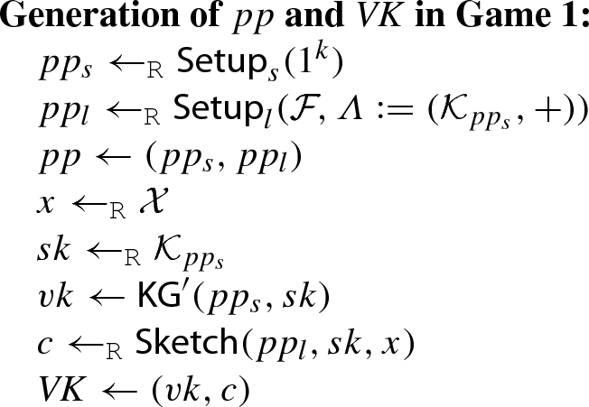
Furthermore, the signing oracle ${\mathcal {O}}_{{\textsf {Sign}}_{{\textsf {FS}}}}(m)$ generates a signature $\sigma$ as follows:

Game 2 :

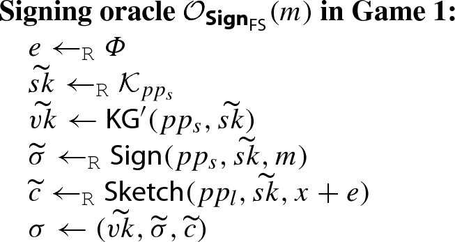
This game is the same as Game 1, except that in the signing oracle, $\widetilde{sk}$ is generated by firstly picking a random “difference” $\Delta sk \in {\mathcal {K}}_{pp_s}$, and then setting $\widetilde{sk}\leftarrow sk + \Delta sk$.

More specifically, the signing oracle ${\mathcal {O}}_{{\textsf {Sign}}_{{\textsf {FS}}}}(m)$ in this game generates a signature $\sigma$ as follows: (The difference from Game 1 is underlined.)

Since the distribution of $\widetilde{sk}$ in Game 2 and that in Game 1 are identical, we have $\Pr [{\textsf {S}}_2] = \Pr [{\textsf {S}}_1]$.

Game 3 :

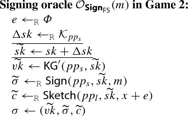
This game is the same as Game 2, except that in the signing oracle, $\widetilde{vk}$ is generated by using vk and $\Delta sk$ via ${\textsf {M}}_{{\textsf {vk}}}$.

More specifically, the signing oracle ${\mathcal {O}}_{{\textsf {Sign}}_{{\textsf {FS}}}}(m)$ in this game generates a signature $\sigma$ as follows: (The difference from Game 2 is underlined.)

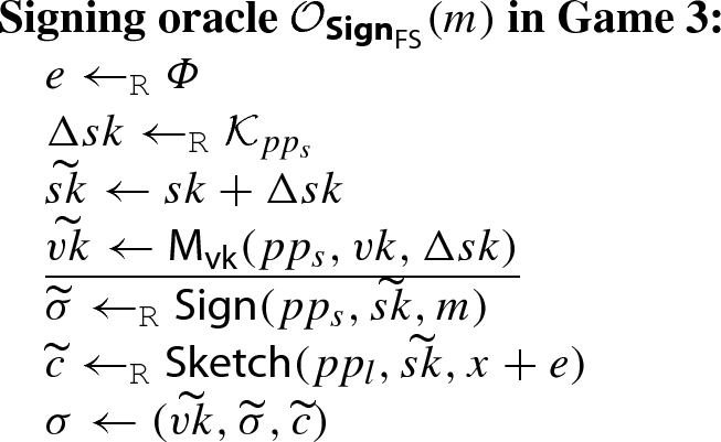
By the property of ${\textsf {M}}_{{\textsf {vk}}}$ [Eq. (2)], the distribution of $\widetilde{vk}$ in Game 3 and that in Game 2 are identical, and thus we have $\Pr [{\textsf {S}}_3] = \Pr [{\textsf {S}}_2]$.

Game 4 :

This game is the same as Game 3, except that in the signing oracle, $\widetilde{c}$ is generated by using c, e, and $\Delta sk$, via the auxiliary algorithm ${\textsf {M}}_{\textsf {c}}$ of the linear sketch scheme ${\mathcal {S}}$.

More specifically, the signing oracle ${\mathcal {O}}_{{\textsf {Sign}}_{{\textsf {FS}}}}(m)$ in this game generates a signature $\sigma$ as follows: (The difference from Game 3 is underlined.)

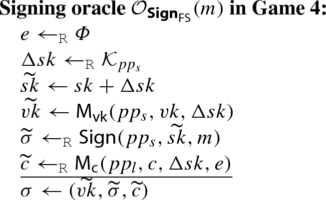
By the linearity of the linear sketch scheme ${\mathcal {S}}$, the distribution of $\widetilde{c}$ generated in the signing oracle in Game 4 and that in Game 3 are statistically indistinguishable. We can apply this statistical indistinguishability query-by-query, to conclude that ${\mathcal {A}}$’s view in Game 4 and that in Game 3 are statistically indistinguishable.¹³ This guarantees that $|\Pr [{\textsf {S}}_4] - \Pr [{\textsf {S}}_3]|$ is negligible.

Game 5 :

This game is the same as Game 4, except that the sketch c contained in ${ VK}$ is generated by the simulator ${\textsf {Sim}}$ (without using $x \in {\mathcal {X}}$ or $sk \in {\mathcal {K}}_{pp_s}$), whose existence is guaranteed by the weak simulatability of the linear sketch scheme ${\mathcal {S}}$.

More specifically, in this game, the public parameter pp and the verification key ${ VK}$ are generated as follows: (The difference from Game 4 is underlined.)

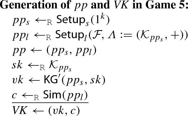
(We no longer pick $x \in {\mathcal {X}}$, because it is not used in Game 5.) Now, we show that due to the weak simulatability of the linear sketch scheme ${\mathcal {S}}$, there exists a polynomial $u = u(k)$ and a negligible function $\epsilon = \epsilon (k)$ such that $\Pr [{\textsf {S}}_4] \le u \cdot \Pr [{\textsf {S}}_5] + \epsilon$ holds. To see this, let $pp_s \leftarrow _{{\texttt {R}}}{\textsf {Setup}}_s(1^{k})$, and let $\varLambda = ({\mathcal {K}}_{pp_s}, +)$ be the abelian group that describes the secret key space of $\varSigma$. Then, consider the PPTA adversary ${\mathcal {B}}'$ that has $pp_s$ hardwired, takes as input a tuple $(pp_l, sk, c)$ that is generated by either

$$\begin{aligned} {\mathcal {D}}_{\mathrm{real}}&= \left\{ ~\begin{array}{l} pp_l \leftarrow _{{\texttt {R}}}{\textsf {Setup}}_l({\mathcal {F}}, \varLambda );\\ x \leftarrow _{{\texttt {R}}}{\mathcal {X}};~ sk \leftarrow _{{\texttt {R}}}{\mathcal {K}}_{pp_s};\\ c \leftarrow _{{\texttt {R}}}{\textsf {Sketch}}(pp_l, sk, x) \end{array}{:}\,(pp_l, sk, c)~\right\} ~~~\text {or}\\ {\mathcal {D}}_{\mathrm{sim}}&= \left\{ ~\begin{array}{l} pp_l \leftarrow _{{\texttt {R}}}{\textsf {Setup}}_l({\mathcal {F}}, \varLambda );\\ sk \leftarrow _{{\texttt {R}}}{\mathcal {K}}_{pp_s};~c \leftarrow _{{\texttt {R}}}{\textsf {Sim}}(pp_l) \end{array}{:}\,(pp_l, sk, c)~\right\} , \end{aligned}$$

simulates Game 4 for ${\mathcal {A}}$ by using these values,¹⁴ and outputs 1 if and only if ${\mathcal {A}}$ succeeds in forging a signature. Then, it is straightforward to see that if the input $(pp_l, sk, c)$ to ${\mathcal {B}}'$ comes from the distribution ${\mathcal {D}}_{\mathrm{real}}$ (resp. ${\mathcal {D}}_{\mathrm{sim}}$), then ${\mathcal {B}}'$ simulates Game 4 (resp. Game 5) in which $pp_s$ is the one hardwired in ${\mathcal {B}}'$, perfectly for ${\mathcal {A}}$. Consequently, we have

Also, by the weak simulatability of ${\mathcal {S}}$, it holds that $\Pr [{\mathcal {B}}'({\mathcal {D}}_{\mathrm{real}}) = 1] \le u \cdot \Pr [{\mathcal {B}}'({\mathcal {D}}_{\mathrm{sim}}) = 1] + \epsilon$. Hence, by the linearity of expectation, we obtain

$$\begin{aligned} \Pr [{\textsf {S}}_4] \le u \cdot \Pr [{\textsf {S}}_5] + \epsilon . \end{aligned}$$

Putting everything together, we can estimate an upperbound of ${\mathcal {A}}$’s ${\texttt {EUF-CMA}}$ advantage as follows:

$$\begin{aligned}&{\textsf {Adv}}^{{\texttt {EUF-CMA}}}_{\varSigma _{{\textsf {FS}}}, {\mathcal {F}}, {\mathcal {A}}}(k) = \Pr [{\textsf {S}}_1]\\&\quad \le \sum _{i \in [3]} \Bigl | \Pr [{\textsf {S}}_i] - \Pr [{\textsf {S}}_{i+1}] \Bigr | + \Pr [{\textsf {S}}_4]\\&\quad \le \sum _{i \in [3]} \Bigl | \Pr [{\textsf {S}}_i] - \Pr [{\textsf {S}}_{i+1}] \Bigr | + u(k) \cdot \Pr [{\textsf {S}}_5] + \epsilon (k),\\&\quad \le u(k) \cdot \Pr [{\textsf {S}}_5] + \epsilon '(k), \end{aligned}$$

where u(k) is a polynomial and $\epsilon (k)$ is a negligible function that are both due to the weak simulatability of the linear sketch scheme ${\mathcal {S}}$ as seen above, and $\epsilon '$ is another negligible function such that $\epsilon ' = \epsilon + |\Pr [{\textsf {S}}_3] - \Pr [{\textsf {S}}_4]|$. (Recall that $\Pr [{\textsf {S}}_1] = \Pr [{\textsf {S}}_2] = \Pr [{\textsf {S}}_3]$.)

Hence, in order to complete the proof, it is sufficient to show that $\Pr [{\textsf {S}}_5]$ is negligible. We show this by relying on the $\varPhi ^{{\text {add}}}\texttt {-}{\texttt {RKA}}^*$ security of the underlying signature scheme $\varSigma$. Specifically, using ${\mathcal {A}}$ as a building block, we construct the following PPTA adversary ${\mathcal {B}}$ that attacks the $\varPhi ^{{\text {add}}}\texttt {-}{\texttt {RKA}}^*$ security of the underlying signature scheme $\varSigma$:

• ${\mathcal {B}}^{{\mathcal {O}}_{{\textsf {Sign}}}(\cdot ,\cdot )}(pp_s, vk){:}$ Let $\varLambda := ({\mathcal {K}}_{pp_s}, +)$. ${\mathcal {B}}$ first generates $pp_l \leftarrow _{{\texttt {R}}}{\textsf {Setup}}_l({\mathcal {F}},\varLambda )$ and sets $pp \leftarrow (pp_s, pp_l)$. Next, ${\mathcal {B}}$ computes $c \leftarrow _{{\texttt {R}}}{\textsf {Sim}}(pp_l)$, and then sets ${ VK} \leftarrow (vk, c)$. Then, ${\mathcal {B}}$ runs ${\mathcal {A}}(pp, { VK})$.

  For each signing query m from ${\mathcal {A}}$, ${\mathcal {B}}$ responds as follows:

  • 1. Pick $e \leftarrow _{{\texttt {R}}}\varPhi$ and $\Delta sk \leftarrow _{{\texttt {R}}}{\mathcal {K}}_{pp_s}$.

  • 2. Submit $(\phi ^{{\text {add}}}_{\Delta sk}, m)$ to its own RKA-signing oracle ${\mathcal {O}}_{{\textsf {Sign}}}$, and receive the result $\widetilde{\sigma }$. (Note that by definition, $\widetilde{\sigma }$ is computed by $\widetilde{\sigma }\leftarrow _{{\texttt {R}}}{\textsf {Sign}}(pp_s, sk + \Delta sk, m)$, where sk is the original signing key corresponding to vk that ${\mathcal {B}}$ received.)

  • 3. Compute $\widetilde{vk}\leftarrow {\textsf {M}}_{{\textsf {vk}}}(pp_s, vk, \Delta sk)$ and $\widetilde{c}\leftarrow _{{\texttt {R}}}{\textsf {M}}_{\textsf {c}}(pp_l, c, \Delta sk, e)$.

  • 4. Return $\sigma = (\widetilde{vk}, \widetilde{\sigma }, \widetilde{c})$ to ${\mathcal {A}}$ as the result of the signing query.

  When ${\mathcal {A}}$ outputs $(m', \sigma ' = (\widetilde{vk}', \widetilde{\sigma }', \widetilde{c}'))$ and terminates, ${\mathcal {B}}$ computes $\Delta sk' \leftarrow {\textsf {DiffRec}}(pp_l, c, \widetilde{c}')$, and terminates with output $(\phi ^{{\text {add}}}_{\Delta sk'}, m', \widetilde{\sigma }')$.

The above completes the description of ${\mathcal {B}}$. It is not hard to see that ${\mathcal {B}}$ perfectly simulates Game 5 for ${\mathcal {A}}$. In particular, ${\mathcal {B}}$ generates pp and ${ VK} = (vk, c)$ in exactly the same way as Game 5. Furthermore, since ${\mathcal {B}}$ can ask a RKA-signing query of the form $(\phi ^{{\text {add}}}_{\Delta sk}, m)$ in the $\varPhi ^{{\text {add}}}\texttt {-}{\texttt {RKA}}^*$ experiment and is given a signature $\widetilde{\sigma }$ computed by using the “shifted” secret key $sk + \Delta sk$, we can view $sk + \Delta sk$ as $\widetilde{sk}$ generated for answering each signing query in Game 5. Note also that the “used messages list” ${\mathcal {Q}}$ by ${\mathcal {A}}$ and that of ${\mathcal {B}}$ are identical.

We finally show that whenever ${\mathcal {A}}$ succeeds in outputting a successful forgery pair $(m', \sigma ' = (\widetilde{vk}', \widetilde{\sigma }', \widetilde{c}'))$ such that ${\textsf {Ver}}_{{\textsf {FS}}}(pp, { VK}, m', \sigma ') = \top$, ${\mathcal {B}}$ also succeeds in outputting a successful forgery $(\phi ^{{\text {add}}}_{\Delta sk'}, m', \widetilde{\sigma }')$, such that

$$\begin{aligned}&{\textsf {Ver}}(pp_s, {\textsf {KG}}'(pp_s, sk + \Delta sk'), m', \widetilde{\sigma }') = \top \nonumber \\&\quad \text {where}~~\Delta sk' = {\textsf {DiffRec}}(pp_l, c, \widetilde{c}'). \end{aligned}$$

(8)

To see this, note that ${\textsf {Ver}}_{{\textsf {FS}}}(pp, { VK}, m', \sigma ') = \top$ implies that ${\textsf {Ver}}(pp_s, \widetilde{vk}', m', \widetilde{\sigma }') = \top$, ${\textsf {DiffRec}}(pp_l, c, \widetilde{c}') = \Delta sk'$, and ${\textsf {M}}_{{\textsf {vk}}}(pp_s, vk, \Delta sk') = \widetilde{vk}'$ hold. The last condition implies $\widetilde{vk}' = {\textsf {KG}}'(pp_s, sk + \Delta sk')$ due to the weak homomorphic property of $\varSigma$. Thus, if ${\mathcal {A}}$’s output $(m', \sigma ')$ satisfies the condition of violating the ${\texttt {EUF-CMA}}$ security of $\varSigma _{{\textsf {FS}}}$, ${\mathcal {B}}$’s output $(\phi ^{{\text {add}}}_{\Delta sk'}, m', \widetilde{\sigma }')$ satisfies the condition of violating the $\varPhi ^{{\text {add}}}\texttt {-}{\texttt {RKA}}^*$ security of the underlying signature scheme $\varSigma$. Hence, we have ${\textsf {Adv}}^{\varPhi ^{{\text {add}}}\texttt {-}{\texttt {RKA}}^*}_{\varSigma , {\mathcal {B}}}(k) = \Pr [{\textsf {S}}_5]$. Since $\varSigma$ is assumed to be $\varPhi ^{{\text {add}}}\texttt {-}{\texttt {RKA}}^*$ secure and ${\mathcal {B}}$ is a PPTA, we can conclude that $\Pr [{\textsf {S}}_5]$ is negligible.

At this point, we have shown that ${\textsf {Adv}}^{{\texttt {EUF-CMA}}}_{\varSigma _{{\textsf {FS}}}, {\mathcal {F}}, {\mathcal {A}}}(k)$ is upperbounded to be negligible. This completes the proof of Theorem 2. $\square$

6 First instantiation

This and next sections give the concrete instantiations of our generic construction of a fuzzy signature scheme given in Sect. 5. In this section, we give our first instantiation based on the Waters signature scheme [36] that uses bilinear groups and the security is proven in the standard model. One strong requirement of this instantiation is that it needs to assume that the fuzzy data is distributed uniformly. (This requirement is relaxed in our second instantiation given in the next section.)

The rest of this section is organized as follows. Since we treat real numbers in our instantiations (in this and next sections), below we first clarify how we treat real numbers. Then in Sect. 6.1, we first specify a concrete fuzzy key setting ${\mathcal {F}}_{1}$ for which our first instantiation is constructed. Next, in Sect. 6.2, we provide some mathematical preliminaries. Armed with them, in Sects. 6.3 and 6.4, we show the concrete linear sketch scheme ${\mathcal {S}}_{{\texttt {CRT}}}$ for ${\mathcal {F}}_{1}$ and the signature scheme $\varSigma _{{\texttt {MWS}}}$, respectively, which are used to instantiate the building blocks of our generic construction. The final description of the first instantiation of our fuzzy signature scheme, $\varSigma _{{\textsf {FS}}1}$, is given in Sect. 6.5.

On the treatment of real numbers. In this and next sections, we use real numbers to represent and process fuzzy data. We assume that a suitable representation with sufficient accuracy is chosen to encode the real numbers whenever they need to be treated by the considered algorithms.

Concretely, we assume that the significand of all real numbers is expressed in an a priori fixed length (in bits) $\lambda$, where $\lambda$ is some natural number that is a polynomial of a security parameter $k$. That is, a real number is expressed in the form $\frac{m}{2^{\gamma }}$, where m is a $\lambda$-bit integer that represents the significand and $-\,\gamma \in {\mathbb {Z}}$ is the exponent. (For ease of treatment of decimal numbers, we use the convention that a positive $\gamma$ implies a negative exponent.) Furthermore, if real numbers are involved in some arithmetic operations such as addition and multiplication, then the rounding-down operation is naturally applied to the significand of the resulting number, so that the result is always expressed in the above form (i.e., its significand is expressed with $\lambda$ bits). We stress that this setting is natural, taking computer implementations into account.

For example, if we multiply a real number $x = \frac{m}{2^{\gamma }}$ (where m is a $\lambda$-bit integer and $0 \le \gamma \le \lambda$) with an n-bit integer a (where $n \le \gamma$), then the resulting number $x \cdot a$ of the multiplication of x and a is treated as

$$\begin{aligned} \Bigl \lfloor \frac{m \cdot a}{2^n} \Bigr \rfloor \cdot 2^{-(\gamma -n)}. \end{aligned}$$

(9)

That is, its significand is a $\lambda$-bit integer $\lfloor \frac{m \cdot a}{2^n} \rfloor$ and its exponent is $- (\gamma - n)$. This might not look straightforward at first glance, but note that the significand $\lfloor \frac{m \cdot a}{2^n} \rfloor$ is the result of the multiplication $m \cdot a$ rounded down to have a $\lambda$-bit precision (the denominator $2^n$ is due to the fact that a is an n-bit integer). The exponent is correspondingly “shifted” to take into account that a is an n-bit integer. See Fig. 5 for an illustration for the calculation of $x \cdot a$. [Such multiplication of a real number in [0, 1) with an integer appears in our concrete instantiations of linear sketch schemes in Sects. 6.3 and 7.2 (and thus in the final descriptions of our concrete fuzzy signature schemes that appear in Sects. 6.5 and 7.3).]

Fig. 5

An illustration of multiplication of a real number $x = \frac{m}{2^{\gamma }}$ and an n-bit integer a

Fig. 6

The linear sketch scheme ${\mathcal {S}}_{{\texttt {CRT}}} = ({\textsf {Setup}}, {\textsf {Sketch}}, {\textsf {DiffRec}})$ for the fuzzy key setting ${\mathcal {F}}_{1}$ (left), and the auxiliary algorithms ${\textsf {M}}_{\textsf {c}}$ for showing linearity and the simulator ${\textsf {Sim}}$ for showing weak simulatability (right). In the figure, all addition are done in ${\mathbb {R}}^n_{\mathbf{w }}$, and $\ell ' = \lambda - \lceil k/n \rceil$

6.1 Specific fuzzy key setting

Here, we specify a concrete fuzzy key setting ${\mathcal {F}}_{1} = (({\textsf {d}},X), t, {\mathcal {X}}, \varPhi , \epsilon )$ for which our first fuzzy signature scheme $\varSigma _{{\textsf {FS}}1}$ is constructed.

Metric space$({\textsf {d}}, X)$.:

We define the space X by $X := [0,1)^n \subset {\mathbb {R}}^n$, where n is a parameter specified by the context (e.g., an object from which we measure fuzzy data). We use the $L_{\infty }$-distance as the distance function ${\textsf {d}}: X \times X \rightarrow {\mathbb {R}}$. Namely, for $\mathbf{x }= (x_1, \dots , x_n) \in X$ and $\mathbf{x }' = (x'_1, \dots , x'_n) \in X$, we define ${\textsf {d}}(\mathbf{x }, \mathbf{x }') := \Vert \mathbf{x }- \mathbf{x }' \Vert _{\infty } := \max _{i \in [n]} |x_i - x'_i|$. Note that X forms an abelian group with respect to

coordinate-wise addition (modulo 1).

Thresholdt.:

For a security parameter $k$, we define the threshold $t \in {\mathbb {R}}$ so that

$$\begin{aligned} k= \lfloor -n \log _2 (2t) \rfloor . \end{aligned}$$

(10)

Looking ahead, this guarantees that the algorithm “${\textsf {WGen}}$” that we will introduce in the next subsection, is a PTA in $k$.

Furthermore, we require that $n = O(\log _2 k)$, so that $2^n$ can be considered to be upperbounded by some polynomial of k. Looking ahead, this property is used in showing the weak simulatability of the linear sketch scheme ${\mathcal {S}}_{{\texttt {CRT}}}$.

We do not directly show that ${\texttt {FAR}}$ is negligible here, because it is indirectly implied by the ${\texttt {EUF-CMA}}$ security of our proposed fuzzy signature scheme.

Distribution${\mathcal {X}}$.:

The uniform distribution over a “discretized” version of $X = [0,1)^n$. Specifically, let $\lambda \in {\mathbb {N}}$ be the natural number that denotes the representation length of a real number as introduced at the beginning of this section. We require that each coordinate $x_i$ of a data $\mathbf{x }= (x_1,\dots ,x_n) \in X$ is distributed as $\{j \leftarrow _{{\texttt {R}}}{\mathbb {Z}}_{2^{\lambda }}{:}\,\frac{j}{2^{\lambda }}\}$.

Furthermore, we require $\lambda$ to be sufficiently large (at least k / n).

Error distribution$\varPhi$and Error parameter$\epsilon$.:

$\varPhi$ can be any efficiently samplable (according to k) distribution over X such that ${\texttt {FRR}}\le \epsilon$ for all $x \in X$.

6.2 Mathematical preliminaries

Group isomorphism based on Chinese remainder theorem. Let $n \in {\mathbb {N}}$. Let $w_1, \dots , w_n \in {\mathbb {N}}$ be positive integers with the same bit length (i.e., $\lceil \log _2 w_1 \rceil = \dots = \lceil \log _2 w_n \rceil$), such that

$$\begin{aligned} \forall i \in [n]{:}\,w_i \le \frac{1}{2t}, \quad \text {and} \quad \forall i \ne j \in [n]{:}\,{\texttt {GCD}}(w_i,w_j) = 1, \end{aligned}$$

(11)

and $W = \prod _{i \in [n]} w_i = \varTheta (2^{k})$, where $k$ is defined as in Eq. (10). Note that Eqs. (10) and (11) imply that we have $w_i \le 2^{k/n}$ for all $i \in [n]$.

We assume that there exists a deterministic algorithm ${\textsf {WGen}}$ that on input (t, n) outputs $\mathbf{w }= (w_1, \dots , w_n)$ satisfying the above.

For vectors $\mathbf{v }= (v_1, \dots , v_n) \in {\mathbb {N}}^n$ and $\mathbf{w }= (w_1, \dots w_n) \in {\mathbb {N}}^n$, we define

$$\begin{aligned} \mathbf{v }\bmod \mathbf{w }:= (v_1 \bmod w_1, \dots , v_n \bmod w_n). \end{aligned}$$

(12)

For vectors $\mathbf{v }_1, \mathbf{v }_2 \in {\mathbb {N}}^n$, we define the equivalence relation “$\sim$” by

$$\begin{aligned} \mathbf{v }_1 \sim \mathbf{v }_2 \quad {\mathop {\Longleftrightarrow }\limits ^{\text {def}}} \quad \mathbf{v }_1 \bmod \mathbf{w }= \mathbf{v }_2 \bmod \mathbf{w }, \end{aligned}$$

and let ${\mathbb {Z}}^n_{\mathbf{w }} := {\mathbb {Z}}^n / \sim$ be the quotient set of ${\mathbb {Z}}^n$ by $\sim$. Note that $({\mathbb {Z}}^n_{\mathbf{w }}, +)$ constitutes an abelian group, where the addition is modulo $\mathbf{w }$ as defined in Eq. (12).

Consider the following system of equations: given $\mathbf{v }, \mathbf{w }\in {\mathbb {N}}^n$, find V such that $V \bmod w_i = v_i~(i \in [n])$. According to the Chinese remainder theorem (CRT), the solution V is determined uniquely modulo W. Thus, for a fixed $\mathbf{w }\in {\mathbb {N}}^n$, we can define a mapping ${\textsf {CRT}}_{\mathbf{w }}{:}\,{\mathbb {Z}}^n_{\mathbf{w }} \rightarrow {\mathbb {Z}}_W$ such that ${\textsf {CRT}}_{\mathbf{w }}(\mathbf{v }) = V \in {\mathbb {Z}}_W$. Note that this mapping is a bijection, and we denote by ${\textsf {CRT}}_{\mathbf{w }}^{-1}$ the “inverse” procedure of ${\textsf {CRT}}_{\mathbf{w }}$.

Note that ${\textsf {CRT}}_{\mathbf{w }}$ satisfies the following homomorphism: For all $\mathbf{v }_1, \mathbf{v }_2 \in {\mathbb {Z}}^n_{\mathbf{w }}$, it holds that

$$\begin{aligned} {\textsf {CRT}}_{\mathbf{w }}(\mathbf{v }_1 + \mathbf{v }_2) = {\textsf {CRT}}_{\mathbf{w }}(\mathbf{v }_1) + {\textsf {CRT}}_{\mathbf{w }}(\mathbf{v }_2) \bmod W. \end{aligned}$$

Since ${\textsf {CRT}}_{\mathbf{w }}$ is bijective between ${\mathbb {Z}}^n_{\mathbf{w }}$ and ${\mathbb {Z}}_W$, ${\textsf {CRT}}_{\mathbf{w }}$ is an isomorphism.

Coding and error correction. Let $\mathbf{w }= (w_1, \dots , w_n) \in {\mathbb {N}}^n$ be the n-dimensional vector satisfying the requirements in Eq. (11). Similarly to ${\mathbb {Z}}^n_{\mathbf{w }}$, we define ${\mathbb {R}}^n_{\mathbf{w }} := {\mathbb {R}}^n /\sim$ be the quotient set of real vector space ${\mathbb {R}}^n$ by the equivalence relation $\sim$, where for a real number $y \in {\mathbb {R}}$, we define $r = y \bmod w_i$ by the number such that $\exists n \in {\mathbb {Z}}{:}\,y = nw_i + r$ and $0 \le r < w_i$.

Let ${\textsf {E}}_{\mathbf{w }}{:}\,{\mathbb {R}}^n \rightarrow {\mathbb {R}}^n_{\mathbf{w }}$ be the following function:

$$\begin{aligned} {\textsf {E}}_{\mathbf{w }}(\mathbf{x }) := (w_1 x_1, \dots , w_n x_n) \in {\mathbb {R}}^n_{\mathbf{w }}, \end{aligned}$$

where $\mathbf{x }= (x_1,\dots ,x_n) \in {\mathbb {R}}^n$. Note that it holds that

$$\begin{aligned} {\textsf {E}}_{\mathbf{w }}(\mathbf{x }+ \mathbf{e }) = {\textsf {E}}_{\mathbf{w }}(\mathbf{x }) + {\textsf {E}}_{\mathbf{w }}(\mathbf{e })\quad (\hbox {mod}\ \mathbf{w }). \end{aligned}$$

(13)

Therefore, ${\textsf {E}}_{\mathbf{w }}$ can be viewed as a kind of linear coding.

Let ${\textsf {C}}_{\mathbf{w }}{:}\,{\mathbb {R}}^n_{\mathbf{w }} \rightarrow {\mathbb {Z}}^n_{\mathbf{w }}$ be the following function:

$$\begin{aligned} {\textsf {C}}_{\mathbf{w }}\Bigl (~(y_1,\dots , y_n)~\Bigr ) := \Bigl (~\lfloor y_1 + 0.5 \rfloor , \dots , \lfloor y_n + 0,5 \rfloor ~\Bigr ). \end{aligned}$$

(14)

We note that the round-down operation $\lfloor y_i + 0.5 \rfloor$ in ${\textsf {C}}_{\mathbf{w }}$ can be regarded as a kind of error correction. Specifically, by the conditions in Eq. (11), the following properties are satisfied: For any $\mathbf{x }, \mathbf{x }' \in X$, if $\Vert \mathbf{x }- \mathbf{x }' \Vert _{\infty } < t$, then we have

$$\begin{aligned} \Bigl \Vert ~{\textsf {E}}_{\mathbf{w }}(\mathbf{x }) - {\textsf {E}}_{\mathbf{w }}(\mathbf{x }')~\Bigr \Vert _{\infty } < t \cdot \max _{i \in [n]}\{w_i\} \le 0.5. \end{aligned}$$

Therefore, for such $\mathbf{x }, \mathbf{x }'$, it always holds that

$$\begin{aligned} {\textsf {C}}_{\mathbf{w }} \Bigl ( {\textsf {E}}_{\mathbf{w }}(\mathbf{x }) - {\textsf {E}}_{\mathbf{w }}(\mathbf{x }') \Bigr ) = \mathbf{0 }. \end{aligned}$$

(15)

Additionally, for any $\mathbf{x }\in {\mathbb {R}}^n$ and $\mathbf{s }\in {\mathbb {Z}}^n_{\mathbf{w }}$, the following holds:

$$\begin{aligned} {\textsf {C}}_{\mathbf{w }}(\mathbf{x }+ \mathbf{s }) = {\textsf {C}}_{\mathbf{w }}(\mathbf{x }) + \mathbf{s }\quad (\hbox {mod}\ \mathbf{w }). \end{aligned}$$

(16)

6.3 Concrete linear sketch

Let ${\mathcal {F}}_{1} = (({\textsf {d}},X), t, {\mathcal {X}},\varPhi ,\epsilon )$ be the fuzzy key setting defined in Sect. 6.1, and let $\mathbf{w }= (w_1, \dots , w_n) = {\textsf {WGen}}(t,n)$, where n is the dimension of X, and let $W = \prod _{i \in [n]} w_i$. Let ${\textsf {CRT}}_{\mathbf{w }}$, ${\textsf {CRT}}^{-1}_{\mathbf{w }}$, ${\textsf {E}}_{\mathbf{w }}$, and ${\textsf {C}}_{\mathbf{w }}$ be the functions defined in Sect. 6.2. Using these objects, we consider the linear sketch scheme ${\mathcal {S}}_{{\texttt {CRT}}} = ({\textsf {Setup}}, {\textsf {Sketch}}, {\textsf {DiffRec}})$ for ${\mathcal {F}}_{1}$ and the additive group $({\mathbb {Z}}_W, +)$ ($=: \varLambda$), as described in Fig. 6 (left). In the right of the figure, we also describe the auxiliary algorithm ${\textsf {M}}_{\textsf {c}}$ that is used to show the linearity of ${\mathcal {S}}_{{\texttt {CRT}}}$, and the simulator ${\textsf {Sim}}$ that is used to show its weak simulatability.

The setup algorithm ${\textsf {Setup}}$ in this linear sketch scheme actually does nothing, and the main algorithms ${\textsf {Sketch}}$ and ${\textsf {DiffRec}}$ as well as the auxiliary algorithm ${\textsf {M}}_{\textsf {c}}$ are all deterministic. Furthermore, recall that we assume that the decimal part of each coordinate $w_ix_i$ in the computation of ${\textsf {E}}_{\mathbf{w }}(\cdot )$ is rounded down so that its precision is the same as $x_i$. Concretely, since the significand of each $x_i$ is expressed in $\lambda$ bits and $w_i$ is a $(\lceil k/n \rceil )$-bit natural number, the decimal part of each $w_i x_i$ is truncated to $\ell ' := \lambda -\lceil k/n \rceil$ bits. Correspondingly, the simulator also picks an element in ${\mathbb {R}}^n_{\mathbf{w }}$, such that the integer part of each of its coordinates is sampled uniformly from ${\mathbb {Z}}_{w_i}$, and its decimal part is distributed uniformly in $\{\frac{j}{2^{\ell '}} | j \in {\mathbb {Z}}_{2^{\ell '}}\}$.

Remark on hypothetical recovering attacks and why they do not work. Let $s \in {\mathbb {Z}}_W$ and $\mathbf{s }= (s_1,\dots , s_n) := {\textsf {CRT}}^{-1}_{\mathbf{w }}(s) \in {\mathbb {Z}}_{\mathbf{w }}$. Let $c_i = s_i + w_i \cdot x_i \bmod w_i$ be the ith coordinate of a sketch $\mathbf{c }$ output from ${\textsf {Sketch}}(pp, s, \mathbf{x })$, where $\mathbf{x }= (x_1, \dots , x_n) \leftarrow _{{\texttt {R}}}{\mathcal {X}}$, and thus each $w_i$ is of the form $x_i = \frac{j}{2^{\lambda }}$ for some $\lambda$-bit integer j. Notice that in our linear sketch scheme ${\mathcal {S}}_{{\texttt {CRT}}}$, if it were not for the rounding-down operation after multiplication of $w_i$ and $x_i$, it holds that $2^{\lambda } \cdot c_i = 2^{\lambda } \cdot s_i + w_i \cdot j \bmod w_i = 2^{\lambda } \cdot s_i \bmod w_i$. Hence, if furthermore ${\texttt {GCD}}(2^{\lambda }, w_i) = 1$, we can recover $s_i$ from $c_i$ by computing $s_i = (2^{\lambda } \cdot c_i) \cdot (2^{\lambda })^{-1} \bmod w_i$, from which we can also recover $x_i$. (Yasuda et al. [39] pointed out recovering attacks of this kind.)

Similarly, notice that the “decimal” part $c^{(i)}_{\mathrm{de}}$ of $c_i$ is dependent only on $w_i$ and $x_i$. Hence, if it were not for the rounding-down operation after multiplication of $w_i$ and $x_i$, $c^{(i)}_{\mathrm{de}}$ would be $w_i \cdot x_i \bmod 1 = \frac{w_i \cdot j}{2^{\lambda }} \bmod 1$. This would in turn imply $2^{\lambda } \cdot c^{(i)}_{\mathrm{de}} = w_i \cdot j \bmod 2^{\lambda }$. If furthermore ${\texttt {GCD}}(2^{\lambda }, w_i) = 1$, then we can calculate $(2^{\lambda } \cdot c^{(i)}_{\mathrm{de}}) \cdot (w_i)^{-1} = j \bmod 2^{\lambda }$. Hence, j (and hence $x_i$) could be recovered from $c^{(i)}_{\mathrm{de}}$ as well.

However, such recovering attacks mentioned above do not apply to our proposed linear sketch scheme${\mathcal {S}}_{{\texttt {CRT}}}$due to the rounding-down operation. As explained in the “On the Treatment of Real Numbers” paragraph, since each $w_i$ is a k / n-bit integer, each $x'_i = w_i \cdot x_i$ results in $\lfloor \frac{w_i \cdot j}{2^{\lceil k/n \rceil }} \rfloor \cdot 2^{- (\lambda - \lceil k/n \rceil )}$. Thus, the ith coordinate $c_i$ of $\mathbf{c }$, and its decimal part $c^{(i)}_{\mathrm{de}}$, are actually of the following forms:

$$\begin{aligned} c_i&= s_i + \Bigl \lfloor \frac{w_i \cdot j}{2^{\lceil k/n \rceil }} \Bigr \rfloor \cdot 2^{-(\lambda - \lceil k/n \rceil )} \bmod w_i, \quad \text {and} \quad \\ c^{(i)}_{\mathrm{de}}&= \Bigl \lfloor \frac{w_i \cdot j}{2^{\lceil k/n \rceil }} \Bigr \rfloor \cdot 2^{-(\lambda - \lceil k/n \rceil )} \bmod 1, \end{aligned}$$

for which the above-mentioned methods for calculating $x_i = \frac{j}{2^{\lambda }}$ from $c_i$ (in case ${\texttt {GCD}}(2^{\lambda },w_i) = 1$) are not applicable. In fact, the weak simulatability of ${\mathcal {S}}_{{\texttt {CRT}}}$ that we show in Lemma 7 below implies that if $\mathbf{x }$ is distributed as required in the fuzzy key setting ${\mathcal {F}}_{1}$ (specified in Sect. 6.1) and s is chosen uniformly, then recovering fuzzy data $\mathbf{x }$ or the input s from $\mathbf{c }$ is not possible (except for a negligible probability).

The following lemma guarantees that our construction ${\mathcal {S}}_{{\texttt {CRT}}}$ satisfies all the requirements.

Lemma 7

The linear sketch scheme ${\mathcal {S}}_{{\texttt {CRT}}}$ in Fig. 6 (left) satisfies Definition 12.

Proof of Lemma 7

We firstly show correctness, then linearity, and finally weak simulatability.

Correctness. The correctness of ${\mathcal {S}}_{{\texttt {CRT}}}$ follows from the properties of the functions ${\textsf {CRT}}_{\mathbf{w }}$, ${\textsf {E}}_{\mathbf{w }}$, and ${\textsf {C}}_{\mathbf{w }}$. Specifically, let $\mathbf{x }, \mathbf{x }' \in X$ be such that ${\textsf {d}}(\mathbf{x }, \mathbf{x }') = \Vert \mathbf{x }- \mathbf{x }'\Vert _{\infty } < t$. Let pp be a public parameter output by ${\textsf {Setup}}$, let $s, \Delta s \in {\mathbb {Z}}_W$, and let $\mathbf{s }= {\textsf {CRT}}_{\mathbf{w }}^{-1}(s)$ and $\Delta \mathbf{s }= {\textsf {CRT}}_{\mathbf{w }}^{-1}(\Delta s)$. Furthermore, let $\mathbf{c }= {\textsf {Sketch}}(pp, s, \mathbf{x }) = (\mathbf{s }+ {\textsf {E}}_{\mathbf{w }}(\mathbf{x })) \bmod \mathbf{w }$ and $\mathbf{c }' = {\textsf {Sketch}}(pp, s + \Delta s, \mathbf{x }') = (\mathbf{s }+ \Delta \mathbf{s }+ {\textsf {E}}_{\mathbf{w }}(\mathbf{x }')) \bmod \mathbf{w }$. Then, we have

$$\begin{aligned} {\textsf {C}}_{\mathbf{w }}(\mathbf{c }' - \mathbf{c })&= {\textsf {C}}_{\mathbf{w }} \Bigl (\mathbf{s }+ \Delta \mathbf{s }+ {\textsf {E}}_{\mathbf{w }}(\mathbf{x }') - (\mathbf{s }+ {\textsf {E}}_{\mathbf{w }}(\mathbf{x })) \Bigr )\\&{\mathop {=}\limits ^{(*)}} \Delta \mathbf{s }+ {\textsf {C}}_{\mathbf{w }} \Bigl ( {\textsf {E}}_{\mathbf{w }}(\mathbf{x }') - {\textsf {E}}_{\mathbf{w }}(\mathbf{x }) \Bigr )\\&{\mathop {=}\limits ^{(\dag )}} \Delta \mathbf{s }, \end{aligned}$$

where (*) is due to Eq. (16) (we omit to write “$\bmod ~\mathbf{w }$”), and (†) is due to Eq. (15) and $\Vert \mathbf{x }- \mathbf{x }'\Vert _{\infty } < t$. Thus,

$$\begin{aligned}&{\textsf {DiffRec}}(pp, \mathbf{c }, \mathbf{c }')\\&\quad = {\textsf {DiffRec}}\Bigl (pp, {\textsf {Sketch}}(pp, s, \mathbf{x }), {\textsf {Sketch}}(pp, s + \Delta s, \mathbf{x }') \Bigr )\\&\quad = {\textsf {CRT}}_{\mathbf{w }} \Bigl ({\textsf {C}}_{\mathbf{w }}(\mathbf{c }' - \mathbf{c }) \Bigr )\\&\quad = {\textsf {CRT}}_{\mathbf{w }}(\Delta \mathbf{s })\\&\quad = \Delta s, \end{aligned}$$

which shows that the correctness condition [Eq. (5)] is satisfied.

Linearity. We consider the auxiliary algorithm ${\textsf {M}}_{\textsf {c}}$ as described in Fig. 6 (right-top). To see that ${\textsf {M}}_{\textsf {c}}$ satisfies the required property, let $\mathbf{x }, \mathbf{e }\in {\mathbb {R}}^n_{\mathbf{w }}$ and $s, \Delta s \in {\mathbb {Z}}_W$, and let $\mathbf{s }= {\textsf {CRT}}_{\mathbf{w }}^{-1}(s)$ and $\Delta \mathbf{s }= {\textsf {CRT}}_{\mathbf{w }}^{-1}(\Delta s)$. Then, note that ${\textsf {Sketch}}(pp, s, \mathbf{x }) = (\mathbf{s }+ {\textsf {E}}_{\mathbf{w }}(\mathbf{x })) \bmod \mathbf{w }$ and ${\textsf {CRT}}_{\mathbf{w }}^{-1}(s + \Delta s) = (\mathbf{s }+ \Delta \mathbf{s }) \bmod \mathbf{w }$. Thus, it holds that

$$\begin{aligned}&{\textsf {M}}_{\textsf {c}}\Bigl (pp, {\textsf {Sketch}}(pp, s, \mathbf{x }), \Delta s, \mathbf{e }\Bigr )\\&\quad = \Bigl ( \mathbf{s }+ {\textsf {E}}_{\mathbf{w }}(\mathbf{x }) + \Delta \mathbf{s }+ {\textsf {E}}_{\mathbf{w }}(\mathbf{e }) \Bigr ) \bmod \mathbf{w }\\&\quad {\mathop {=}\limits ^{(*)}} \Bigl ( \mathbf{s }+ \Delta \mathbf{s }+ {\textsf {E}}_{\mathbf{w }}(\mathbf{x }+ \mathbf{e }) \Bigr ) \bmod \mathbf{w }\\&\quad = {\textsf {Sketch}}(pp, s + \Delta s, \mathbf{x }+ \mathbf{e }), \end{aligned}$$

where (*) is due to the linearity of ${\textsf {E}}_{\mathbf{w }}$ [Eq. (13)]. This equation implies that the two distributions in Eq. (6) are identical, and hence the linearity is satisfied.

Weak simulatability. We consider the simulator ${\textsf {Sim}}$ as described in Fig. 6 (right-bottom). Let ${\mathcal {D}}_{\mathrm{real}}$ and ${\mathcal {D}}_{\mathrm{sim}}$ be the distributions for the weak simulatability of ${\mathcal {S}}_{{\texttt {CRT}}}$, which are defined as follows:

$$\begin{aligned} {\mathcal {D}}_{\mathrm{real}}&:= \left\{ ~\begin{array}{l} \mathbf{x }\leftarrow _{{\texttt {R}}}{\mathcal {X}};~s \leftarrow _{{\texttt {R}}}{\mathbb {Z}}_W;\\ ~\mathbf{c }\leftarrow {\textsf {CRT}}^{-1}_{\mathbf{w }}(s) + {\textsf {E}}_{\mathbf{w }}(\mathbf{x })\end{array}{:}\,(s, \mathbf{c })~\right\} \\&=\left\{ ~\begin{array}{l} \mathbf{j }\leftarrow _{{\texttt {R}}}({\mathbb {Z}}_{2^{\lambda }})^n;~\mathbf{x }\leftarrow 2^{-\lambda } \cdot \mathbf{j };\\ s \leftarrow _{{\texttt {R}}}{\mathbb {Z}}_W;~\mathbf{c }\leftarrow {\textsf {CRT}}^{-1}_{\mathbf{w }}(s) + {\textsf {E}}_{\mathbf{w }}(\mathbf{x }) \end{array}{:}\,(s, \mathbf{c })~\right\} ,\\ {\mathcal {D}}_{\mathrm{sim}}&:= \Bigl \{~s \leftarrow _{{\texttt {R}}}{\mathbb {Z}}_W;~\mathbf{c }\leftarrow _{{\texttt {R}}}{\textsf {Sim}}(pp): (s, \mathbf{c })~\Bigr \}\\&= \left\{ ~\begin{array}{l} s \leftarrow _{{\texttt {R}}}{\mathbb {Z}}_W;~\mathbf{c }_{\mathrm{in}} \leftarrow _{{\texttt {R}}}{\mathbb {Z}}^n_{\mathbf{w }};~\mathbf{j }\leftarrow _{{\texttt {R}}}({\mathbb {Z}}_{2^{\ell '}})^n;\\ \mathbf{c }_{\mathrm{de}} \leftarrow 2^{-{\ell '}} \cdot \mathbf{j };~\mathbf{c }\leftarrow \mathbf{c }_{\mathrm{in}} + \mathbf{c }_{\mathrm{de}} \end{array}{:}\,(s, \mathbf{c })~\right\} , \end{aligned}$$

where $pp = \varLambda = ({\mathbb {Z}}_W, +)$ and $\ell ' = \lambda - \lceil k/n \rceil$. We will show that for any (even computationally unbounded) algorithm ${\mathcal {A}}$, the following inequality holds:

$$\begin{aligned} \Pr [{\mathcal {A}}({\mathcal {D}}_{\mathrm{real}}) = 1] \le 2^n \cdot \Pr [{\mathcal {A}}({\mathcal {D}}_{\mathrm{sim}}) = 1]. \end{aligned}$$

(17)

Recall that we are requiring that $n = O(\log _2 k)$, equivalently $2^n$ is smaller than some polynomial of k, and hence Eq. (17) implies weak simulatability.

Instead of directly showing Eq. (17) for any algorithm ${\mathcal {A}}$, we first slightly simplify the setting. Specifically, consider the following two distributions ${\mathcal {D}}'_{\mathrm{real}}$ and ${\mathcal {D}}'_{\mathrm{sim}}$:

$$\begin{aligned} {\mathcal {D}}'_{\mathrm{real}}&:= \Bigl \{~\mathbf{j }\leftarrow _{{\texttt {R}}}({\mathbb {Z}}_{2^{\lambda }})^n;~\mathbf{x }\leftarrow _{{\texttt {R}}}2^{-\lambda } \cdot \mathbf{j };~\mathbf{x }' \leftarrow {\textsf {E}}_{\mathbf{w }}(\mathbf{x }){:}\,\mathbf{x }'~\Bigr \}\\ {\mathcal {D}}'_{\mathrm{sim}}&:= \left\{ ~\begin{array}{l} \mathbf{x }'_{\mathrm{in}} \leftarrow _{{\texttt {R}}}{\mathbb {Z}}^n_{\mathbf{w }};~\mathbf{j }\leftarrow _{{\texttt {R}}}({\mathbb {Z}}_{2^{\ell '}})^n;\\ \mathbf{x }'_{\mathrm{de}} \leftarrow 2^{-{\ell '}} \cdot \mathbf{j };~\mathbf{x }' \leftarrow \mathbf{x }'_{\mathrm{in}} + \mathbf{x }'_{\mathrm{de}} \end{array}{:}\,\mathbf{x }'~\right\} . \end{aligned}$$

We now show that for any algorithm ${\mathcal {A}}$ considered for weak simulatability, there exists a corresponding algorithm ${\mathcal {B}}$ (with almost the same running time as ${\mathcal {A}}$) such that $\Pr [{\mathcal {A}}({\mathcal {D}}_{\mathrm{real}}) = 1] = \Pr [{\mathcal {B}}({\mathcal {D}}'_{\mathrm{real}}) = 1]$ and $\Pr [{\mathcal {A}}({\mathcal {D}}_{\mathrm{sim}}) = 1] = \Pr [{\mathcal {B}}({\mathcal {D}}'_{\mathrm{sim}}) = 1]$. Specifically, ${\mathcal {B}}$ takes $\mathbf{x }' \in {\mathbb {R}}^n_{\mathbf{w }}$ as input, picks $s \in {\mathbb {Z}}_W$ uniformly at random, sets $\mathbf{c }\leftarrow {\textsf {CRT}}^{-1}_{\mathbf{w }}(s) + \mathbf{x }'$, and outputs ${\mathcal {A}}(s, \mathbf{c })$. If $\mathbf{x }'$ that is input to ${\mathcal {B}}$ is sampled from ${\mathcal {D}}'_{\mathrm{real}}$, then the pair $(s, \mathbf{c })$ that ${\mathcal {B}}$ inputs to ${\mathcal {A}}$ is distributed identically to ${\mathcal {D}}_{\mathrm{real}}$, while if $\mathbf{x }'$ is sampled from ${\mathcal {D}}'_{\mathrm{sim}}$, then $(s, \mathbf{c })$ is distributed identically to ${\mathcal {D}}_{\mathrm{sim}}$. (In particular, the “integer part” of $\mathbf{c }$ is uniformly distributed over ${\mathbb {Z}}^n_{\mathbf{w }}$, even if ${\textsf {CRT}}^{-1}_{\mathbf{w }}(s)$ is added.) Clearly, this ${\mathcal {B}}$ satisfies $\Pr [{\mathcal {B}}({\mathcal {D}}'_{\mathrm{real}}) = 1] = \Pr [{\mathcal {A}}({\mathcal {D}}_{\mathrm{real}}) = 1]$ and $\Pr [{\mathcal {B}}({\mathcal {D}}'_{\mathrm{sim}}) = 1] = \Pr [{\mathcal {A}}({\mathcal {D}}_{\mathrm{sim}}) = 1]$.

Hence, in order to show Eq. (17) for any algorithm ${\mathcal {A}}$, it is sufficient to show the following inequality for any algorithm ${\mathcal {B}}$:

$$\begin{aligned} \Pr [{\mathcal {B}}({\mathcal {D}}'_{\mathrm{real}}) = 1] \le 2^n \cdot \Pr [{\mathcal {B}}({\mathcal {D}}'_{\mathrm{sim}}) = 1]. \end{aligned}$$

(18)

Furthermore, notice that ${\mathcal {D}}'_{\mathrm{sim}}$ is nothing but the uniform distribution over the set ${\mathbb {Z}}^n_{\mathbf{w }} \times \{\frac{j}{2^{\ell '}} | j \in {\mathbb {Z}}_{2^{\ell '}}\}^n$, whose size is $\prod _{i \in [n]} (w_i \cdot 2^{\ell '})$. Hence, by applying Lemma 2, we obtain

$$\begin{aligned} \Pr [{\mathcal {B}}({\mathcal {D}}'_{\mathrm{real}}) = 1] \le \prod _{i \in [n]} (w_i \cdot 2^{\ell '}) \cdot 2^{-\mathbf{H }_{\infty }({\mathcal {D}}'_{\mathrm{real}})} \cdot \Pr [{\mathcal {B}}({\mathcal {D}}'_{\mathrm{sim}}) = 1]. \end{aligned}$$

(19)

To complete the proof, we will show

$$\begin{aligned} 2^{-\mathbf{H }_{\infty }({\mathcal {D}}'_{\mathrm{real}})} \le \prod _{i \in [n]} \Bigl (\frac{1}{w_i \cdot 2^{\ell '}} + \frac{1}{2^{\lambda }} \Bigr ). \end{aligned}$$

(20)

Before showing the above, note that Eq. (20) implies that $\prod _{i \in [n]} (w_i \cdot 2^{\ell '}) \cdot 2^{-\mathbf{H }_{\infty }({\mathcal {D}}'_{\mathrm{real}})}$ [appearing in the right hand side of Eq. (19)] is upperbounded as follows:

$$\begin{aligned} \prod _{i \in [n]}(w_i \cdot 2^{\ell '}) \cdot \prod _{i \in [n]}(\frac{1}{w_i \cdot 2^{\ell '}} + \frac{1}{2^{\lambda }}) \le \prod _{i \in [n]}(1 + 2^{\lceil k/n \rceil + \ell ' - \lambda }) = 2^n, \end{aligned}$$

where the inequality uses $w_i \le 2^{\lceil k/n \rceil }$, and the equality uses $\ell ' = \lambda - \lceil k/n \rceil$. Thus, if indeed we can show Eq. (20), then by combining it with Eq. (19), we can obtain Eq. (18).

Hence, it remains to show Eq. (20). For each $i \in [n]$, let ${\mathcal {D}}'^{(i)}_{\mathrm{real}}$ be the distribution of the ith coordinate in ${\mathcal {D}}'_{\mathrm{real}}$. Recall that each $w_i$ is a k / n-bit integer, each $x_i \in [0,1)$ is of the form $\frac{j}{2^{\lambda }}$ where $j \leftarrow _{{\texttt {R}}}{\mathbb {Z}}_{2^{\lambda }}$, and $x'_i$ is a multiplication of $w_i$ and $x_i$. Recall also that $\ell ' = \lambda - k/n$. Hence, ${\mathcal {D}}'^{(i)}_{\mathrm{real}}$ is distributed as follows [see also Eq. (9)]:

$$\begin{aligned} {\mathcal {D}}'^{(i)}_{\mathrm{real}}&= \Bigl \{~j \leftarrow _{{\texttt {R}}}{\mathbb {Z}}_{2^{\lambda }};~x_i \leftarrow 2^{-\lambda } \cdot j{:}\,~\lfloor w_i \cdot x_i \cdot 2^{\ell '} \rfloor \cdot 2^{-\ell '}~\Bigr \}\\&= \Bigl \{~j \leftarrow _{{\texttt {R}}}{\mathbb {Z}}_{2^{\lambda }}{:}\,\lfloor w_i \cdot j \cdot 2^{\ell ' - \lambda } \rfloor \cdot 2^{-\ell '} \Bigr \}. \end{aligned}$$

We can thus calculate $2^{-\mathbf{H }_{\infty }({\mathcal {D}}'_{\mathrm{real}})}$ as follows:

$$\begin{aligned}&2^{-\mathbf{H }_{\infty }({\mathcal {D}}'_{\mathrm{real}})}\nonumber \\&\quad = \prod _{i \in [n]} 2^{-\mathbf{H }_{\infty }({\mathcal {D}}'^{(i)}_{\mathrm{real}})} = \prod _{i \in [n]} \Bigl (~\max _{z \in {\mathbb {R}}_{w_i}} \Pr _{x'_i \leftarrow _{{\texttt {R}}}{\mathcal {D}}'^{(i)}_{\mathrm{real}}}[~x'_i = z~]~\Bigr ) \nonumber \\&\quad =\prod _{i \in [n]} \Bigl (~\max _{z \in {\mathbb {R}}_{w_i}} \Pr _{j \leftarrow _{{\texttt {R}}}{\mathbb {Z}}_{2^{\lambda }}} \Bigl [~\lfloor w_i \cdot j \cdot 2^{\ell ' - \lambda } \rfloor \cdot 2^{-\ell '} = z~\Bigr ]~\Bigr ) \nonumber \\&\quad = \prod _{i \in [n]} \Bigl (~\max _{z \in {\mathbb {R}}_{w_i}} \Pr _{j \leftarrow _{{\texttt {R}}}{\mathbb {Z}}_{2^{\lambda }}} \Bigl [~z \cdot 2^{\ell '} \le w_i \cdot j \cdot 2^{\ell ' - \lambda }< z \cdot 2^{\ell '} + 1~\Bigr ]~\Bigr ) \nonumber \\&\quad = \prod _{i \in [n]} \Bigl (~\max _{z \in {\mathbb {R}}_{w_i}} \Pr _{j \leftarrow _{{\texttt {R}}}{\mathbb {Z}}_{2^{\lambda }}} \Bigl [~\frac{z \cdot 2^{\lambda }}{w_i} \le j < \frac{z \cdot 2^{\lambda }}{w_i} + \frac{2^{\lambda }}{w_i \cdot 2^{\ell '}} \Bigr ]~\Bigr ). \end{aligned}$$

(21)

Now, for each $z \in {\mathbb {R}}_{w_i}$, let $a_z$ be the number of integers that belong to the interval $[\frac{z \cdot 2^{\lambda }}{w_i}, \frac{(z \cdot 2^{\ell '}+ 1) \cdot 2^{\lambda }}{w_i \cdot 2^{\ell '}})$. By definition, the probability appearing in Eq. (21) is $\frac{a_z}{2^{\lambda }}$. Furthermore, the number of integers that belong to an interval [l, r) is at most $r - l + 1$, and thus we have $a_z \le \frac{2^{\lambda }}{w_i \cdot 2^{\ell '}} + 1$. (Note that the right hand side is independent of z.) Using this, we can upperbound $2^{-\mathbf{H }_{\infty }({\mathcal {D}}'_{\mathrm{real}})}$ as follows:

$$\begin{aligned} 2^{-\mathbf{H }_{\infty }({\mathcal {D}}'_{\mathrm{real}})} = \prod _{i \in [n]} \Bigl (\max _{z \in {\mathbb {R}}_{w_i}} \frac{a_z}{2^{\lambda }} \Bigr ) \le \prod _{i \in [n]} \Bigl (\frac{1}{w_i \cdot 2^{\ell '}} + \frac{1}{2^{\lambda }}\Bigr ), \end{aligned}$$

which is exactly Eq. (20), as required. This completes the proof that ${\mathcal {S}}_{{\texttt {CRT}}}$ satisfies weak simulatability, and the entire proof of Lemma 7. $\square$

6.4 Modified Waters signature scheme

Here, we show a variant of the Waters signature scheme [36], which we call the modified Waters signature (MWS) scheme $\varSigma _{{\texttt {MWS}}}$. We then show that $\varSigma _{{\texttt {MWS}}}$ satisfies ${\texttt {EUF-CMA}}$ security and the homomorphic property (Definition 9), which in turn implies that it is $\varPhi ^{{\text {add}}}\texttt {-}{\texttt {RKA}}^*$ secure (due to Lemma 5).

Specific bilinear group generator${{\textsf {BGGen}}}_{{\texttt {MWS}}}$. In the MWS scheme, we use a (slightly) non-standard way for specifying bilinear groups, namely the order p of (symmetric) bilinear groups is generated based on an integer $W = \prod _{i \in [n]} w_i$, where $\mathbf{w }= (w_1, \dots , w_n) \in {\mathbb {N}}^n$ satisfies the conditions in Eq. (11), so that p is the smallest prime satisfying $W| p-1$. More concretely, we consider the following algorithm ${\textsf {PGen}}$ for choosing the order p based on W:

• ${\textsf {PGen}}(W)$: on input $W \in {\mathbb {N}}$, for $i = 1,2, \dots$ check if $p = iW + 1$ is a prime and return p if this is the case. Otherwise, increment $i \leftarrow i +1$ and go to the next iteration.

According to the prime number theorem, the density of primes among the natural numbers that are less than N is roughly $1/ \ln N$, and thus for i’s that are exponentially smaller than W, the probability that $iW + 1$ is a prime can be roughly estimated as $1/\ln W$. Therefore, by using the above algorithm ${\textsf {PGen}}$, one can find a prime p satisfying $W | p -1$ by performing the primality testing for $O(\ln W) = O(k)$ times on average (recall that $W = \varTheta (2^{k})$). Furthermore, if ${\textsf {PGen}}(W)$ outputs p, then it is guaranteed that $p/W = O(k)$. (This fact is used for security.)

Let ${{\textsf {BGGen}}}_{{\texttt {MWS}}}$ denote an algorithm that, given $1^{k}$, runs $\mathbf{w }\leftarrow {\textsf {WGen}}(t,n)$ where t and n are the parameters from the fuzzy data setting ${\mathcal {F}}$ corresponding the security parameter $k$, computes $W \leftarrow \prod _{i \in [n]} w_i$, $p \leftarrow {\textsf {PGen}}(W)$, and outputs a description of bilinear groups ${\mathcal {BG}}= (p, {\mathbb {G}}, {\mathbb {G}}_T, g, e)$, where ${\mathbb {G}}$ and ${\mathbb {G}}_T$ are cyclic groups with order p and $e{:}\,{\mathbb {G}}\times {\mathbb {G}}\rightarrow {\mathbb {G}}_T$ is a bilinear map.

Construction. Using ${{\textsf {BGGen}}}_{{\texttt {MWS}}}$ and the algorithms in the original Waters signature scheme $\varSigma _{{\texttt {Wat}}}= ({\textsf {Setup}}_{{\texttt {Wat}}}, {\textsf {KG}}_{{\texttt {Wat}}}, {\textsf {Sign}}_{{\texttt {Wat}}}, {\textsf {Ver}}_{{\texttt {Wat}}})$ in Fig. 3 (left), the MWS scheme $\varSigma _{{\texttt {MWS}}}= ({\textsf {Setup}}_{{\texttt {MWS}}}, {\textsf {KG}}_{{\texttt {MWS}}}, {\textsf {Sign}}_{{\texttt {MWS}}}, {\textsf {Ver}}_{{\texttt {MWS}}})$ is constructed as in Fig. 7 (left). Note that the component $pp_{{\texttt {Wat}}}$ in a public parameter pp (generated by ${\textsf {Setup}}_{{\texttt {MWS}}}$) is distributed identically to that generated in the original Waters scheme $\varSigma _{{\texttt {Wat}}}$ in which the bilinear group generator ${{\textsf {BGGen}}}_{{\texttt {MWS}}}$ is used. Therefore, $\varSigma _{{\texttt {MWS}}}$ can be viewed as the original Waters scheme $\varSigma _{{\texttt {Wat}}}$, except that

• 1. we specify how to generate the parameter of bilinear groups by ${{\textsf {BGGen}}}_{{\texttt {MWS}}}$, and

• 2. we use a secret key $sk'$ (for the Waters scheme) of the form $sk' = z^{sk} \bmod p$, thereby we change the signing key space from ${\mathbb {Z}}_p$ to ${\mathbb {Z}}_W$.

Because of these changes, it is immediate to see that the MWS scheme inherits the perfect correctness of the Waters signature scheme.

Fig. 7

The modified Waters signature (MWS) scheme $\varSigma _{{\texttt {MWS}}}$ (left), and the auxiliary algorithms $({\textsf {KG}}', {\textsf {M}}_{{\textsf {vk}}}, {\textsf {M}}_{{\textsf {sig}}})$ for showing the homomorphic property (right). Note that the signing algorithm ${\textsf {Sign}}_{{\texttt {MWS}}}$ (resp. the verification algorithm ${\textsf {Ver}}_{{\texttt {MWS}}}$) of the MWS scheme $\varSigma _{{\texttt {MWS}}}$ uses the signing algorithm ${\textsf {Sign}}_{{\texttt {Wat}}}$ (resp. the verification algorithm ${\textsf {Ver}}_{{\texttt {Wat}}}$) of the original Waters scheme $\varSigma _{{\texttt {Wat}}}$ [described in Fig. 3 (left)] as a subroutine

In the following, we show that $\varSigma _{{\texttt {MWS}}}$ satisfies ${\texttt {EUF-CMA}}$ security (based on the CDH assumption with respect to ${{\textsf {BGGen}}}_{{\texttt {MWS}}}$) and the homomorphic property (Definition 9). These properties, combined with Lemma 5, imply that $\varSigma _{{\texttt {MWS}}}$ satisfies $\varPhi ^{{\text {add}}}$-${\texttt {RKA}}^*$ security, and thus satisfies the assumption required in Theorem 2. (One might suspect the plausibility of the CDH assumption with respect to ${{\textsf {BGGen}}}_{{\texttt {MWS}}}$ due to our specific choice of the order p. We discuss it in “Appendix G.”)

Lemma 8

If the CDH assumption holds with respect to ${{\textsf {BGGen}}}_{{\texttt {MWS}}}$, then the MWS scheme $\varSigma _{{\texttt {MWS}}}$ is ${\texttt {EUF-CMA}}$ secure.

Let $pp = (pp_{{\texttt {Wat}}}, z)$ be a public parameter output by ${\textsf {Setup}}_{{\texttt {MWS}}}$, let $D^{(1)}_{pp} = \{sk \leftarrow _{{\texttt {R}}}{\mathbb {Z}}_W; sk' \leftarrow z^{sk} \bmod p{:}\,sk'\}$ and $D^{(2)}_{pp} = \{sk' \leftarrow _{{\texttt {R}}}{\mathbb {Z}}_p{:}\,sk'\}$. Note that the support of $D^{(1)}_{pp}$ is a strict subset of that of $D^{(2)}_{pp}$.

Now, let ${\mathcal {A}}$ be any PPTA adversary attacking the ${\texttt {EUF-CMA}}$ security of the MWS scheme $\varSigma _{{\texttt {MWS}}}$. Let ${\textsf {Expt}}_1$ be the original ${\texttt {EUF-CMA}}$ experiment, i.e., ${\textsf {Expt}}^{{\texttt {EUF-CMA}}}_{\varSigma _{{\texttt {MWS}}},{\mathcal {A}}}(k)$, and let ${\textsf {Expt}}_2$ be the experiment that is defined in the same manner as ${\textsf {Expt}}_1$, except that $sk'$ is sampled according to the distribution $D^{(2)}_{pp}$. For both $i \in \{1,2\}$, let ${\textsf {Adv}}_i$ be the advantage of ${\mathcal {A}}$ (i.e., the probability of ${\mathcal {A}}$ outputting a successful forgery) in ${\textsf {Expt}}_i$. Then, by Lemma 4, we have ${\textsf {Adv}}_1 \le (p/W) \cdot {\textsf {Adv}}_2 = O(k) \cdot {\textsf {Adv}}_2$. Furthermore, it is straightforward to see that succeeding in forging in ${\textsf {Expt}}_2$ is as difficult as succeeding in breaking the ${\texttt {EUF-CMA}}$ security of the original Waters scheme $\varSigma _{{\texttt {Wat}}}$ (in which the bilinear group generator ${{\textsf {BGGen}}}_{{\texttt {MWS}}}$ is used), and thus ${\textsf {Adv}}_2$ is negligible if $\varSigma _{{\texttt {Wat}}}$ is ${\texttt {EUF-CMA}}$ secure.

Finally, due to Waters [36], if the CDH assumption holds with respect to ${{\textsf {BGGen}}}_{{\texttt {MWS}}}$, then the Waters scheme $\varSigma _{{\texttt {Wat}}}$ (in which ${{\textsf {BGGen}}}_{{\texttt {MWS}}}$ is used,) is ${\texttt {EUF-CMA}}$ secure. Hence, ${\textsf {Adv}}_2$ is negligible. Combining all the explanations above proves the lemma. $\square$

Lemma 9

The MWS scheme $\varSigma _{{\texttt {MWS}}}$ is homomorphic (as per Definition 9).

Proof of Lemma 9

Consider the algorithms $({\textsf {KG}}', {\textsf {M}}_{{\textsf {vk}}}, {\textsf {M}}_{{\textsf {sig}}})$ that are described in Fig. 7 (right). ${\textsf {KG}}'$ is the algorithm for showing that this scheme has a simple key generation process. That is, using this algorithm, ${\textsf {KG}}_{{\texttt {MWS}}}$ can be rewritten with the process in Eq. (1). The secret key space is ${\mathbb {Z}}_W$, and $({\mathbb {Z}}_W, +)$ constitutes an abelian group, as required.

Next, it should be easy to see that ${\textsf {M}}_{{\textsf {vk}}}$ satisfies the requirement in Eq. (2). Indeed, let $pp = (pp_{{\texttt {Wat}}}, z)$ be a public parameter, and let $sk, \Delta sk \in {\mathbb {Z}}_W$. Then, it holds that

$$\begin{aligned}&{\textsf {M}}_{{\textsf {vk}}}(pp, {\textsf {KG}}'(pp, sk), \Delta sk) = (g^{z^{sk}})^{z^{\Delta sk}} = g^{z^{sk + \Delta sk}}\\&\quad = {\textsf {KG}}'(pp, sk + \Delta sk), \end{aligned}$$

which is exactly Eq. (2).

Finally, we observe that ${\textsf {M}}_{{\textsf {sig}}}$ satisfies the requirements in Eq. (3). Let $pp = (pp_{{\texttt {Wat}}}, z)$ and $sk, \Delta sk \in {\mathbb {Z}}_W$ as above, and $m = (m_1 \Vert \dots \Vert m_{\ell }) \in \{0,1\}^{\ell }$ be a message to be signed. Let $(\sigma _1, \sigma _2)$ be a signature on the message m that is generated by ${\textsf {Sign}}_{{\texttt {MWS}}}(pp, sk, m; r)$, where $r \in {\mathbb {Z}}_p$ is a randomness. By definition, $\sigma _1$ and $\sigma _2$ are of the form $\sigma _1 = h^{z^{sk}} \cdot (u' \cdot \prod _{i \in [\ell ]}u_i^{m_i})^r$ and $\sigma _2 = g^r$, respectively. Thus, if $\sigma ' = (\sigma '_1, \sigma '_2)$ is output by ${\textsf {M}}_{{\textsf {sig}}}(pp, vk, m, \sigma , \Delta sk)$, then it holds that

$$\begin{aligned} \sigma '_1&= \sigma _1^{z^{\Delta sk}} = h^{z^{sk + \Delta sk}} \cdot \left( u' \cdot \prod _{i \in [\ell ]} u_i^{m_i}\right) ^{r \cdot z^{\Delta sk}},\\ \sigma '_2&= \sigma _2^{z^{\Delta sk}} = g^{r \cdot z^{\Delta sk}}. \end{aligned}$$

This implies $\sigma ' = (\sigma '_1, \sigma '_2) = {\textsf {Sign}}_{{\texttt {MWS}}}(pp, sk + \Delta sk, m; r \cdot z^{\Delta sk})$. Note that for any $\Delta sk \in {\mathbb {Z}}_W$, if $r \leftarrow _{{\texttt {R}}}{\mathbb {Z}}_p$, then $((r \cdot z^{\Delta sk}) \bmod p)$ is uniformly distributed in ${\mathbb {Z}}_p$. This implies that the distributions considered in Eq. (3) are identical. Furthermore, by the property of the MWS scheme (which is inherited from the original Waters scheme [36]), any signature $\sigma ' = (\sigma '_1, \sigma '_2)$ satisfying ${\textsf {Ver}}_{{\texttt {MWS}}}(pp, vk, m, \sigma ') = \top$ must satisfy the property that there exists $r' \in {\mathbb {Z}}_p$ such that ${\textsf {Sign}}_{{\texttt {MWS}}}(pp, sk, m; r') = \sigma '$. Putting everything together implies that for any $sk, \Delta sk \in {\mathbb {Z}}_W$, any message $m \in \{0,1\}^{\ell }$, and any signature $\sigma$ such that ${\textsf {Ver}}_{{\texttt {MWS}}}(pp, vk, m, \sigma ) = \top$, if $vk = {\textsf {KG}}'(pp, sk)$, $vk' = {\textsf {M}}_{{\textsf {vk}}}(pp, vk, \Delta sk)$ and $\sigma ' = {\textsf {M}}_{{\textsf {sig}}}(pp, vk, m, \sigma , \Delta sk)$, then it holds that ${\textsf {Ver}}_{{\texttt {MWS}}}(pp, vk', m, \sigma ') = \top$. Therefore, the requirement regarding Eq. (4) is satisfied as well. This completes the proof of Lemma 9. $\square$

Fig. 8

Our first instantiation of a fuzzy signature scheme $\varSigma _{{\textsf {FS}}1}$. $^{(\dag )}$ The steps involving “${\texttt {Round}}_{\ell }$” enclosed by a box in ${\textsf {KG}}_{{\textsf {FS}}1}$ and ${\textsf {Sign}}_{{\textsf {FS}}1}$ are those at which we perform the “rounding” operation of the decimal part, which we will explain in Sect. 8. (The reader who has not read there is expected to ignore them)

The combination of Lemmas 5, 8, and 9 shows that $\varSigma _{{\texttt {MWS}}}$ satisfies $\varPhi ^{{\text {add}}}\texttt {-}{\texttt {RKA}}^*$ security.

Corollary 1

If the CDH assumption holds with respect to ${{\textsf {BGGen}}}_{{\texttt {MWS}}}$, then the MWS scheme $\varSigma _{{\texttt {MWS}}}$ is $\varPhi ^{{\text {add}}}\texttt {-}{\texttt {RKA}}^*$ secure.

6.5 Full description

Here, we give the full description of our first instantiation of a fuzzy signature scheme, by instantiating the underlying linear sketch and signature schemes in the generic construction, with the concrete linear sketch scheme ${\mathcal {S}}_{{\texttt {CRT}}}$ (given in Sect. 6.3) and the MWS scheme $\varSigma _{{\texttt {MWS}}}$ (given in Sect. 6.4), respectively.

Let $\ell = \ell (k)$ be a positive polynomial that denotes the length of messages. Let ${\mathcal {F}}_{1} = (({\textsf {d}}, X), t, {\mathcal {X}}, \varPhi , \epsilon )$ be the fuzzy key setting defined in Sect. 6.1, where t (and n) are determined according to the security parameter $k$. let $\mathbf{w }= (w_1, \dots , w_n) = {\textsf {WGen}}(t,n)$, where n is the dimension of X, and let $W = \prod _{i \in [n]} w_i$. Let ${\textsf {CRT}}_{\mathbf{w }}$, ${\textsf {CRT}}^{-1}_{\mathbf{w }}$, ${\textsf {E}}_{\mathbf{w }}$, and ${\textsf {C}}_{\mathbf{w }}$ be the functions defined in Sect. 6.2. Let ${{\textsf {BGGen}}}_{{\texttt {MWS}}}$ be the bilinear group generator defined in Sect. 6.4. Then, using these ingredients, our first proposed fuzzy signature scheme $\varSigma _{{\textsf {FS}}1}= ({\textsf {Setup}}_{{\textsf {FS}}1}, {\textsf {KG}}_{{\textsf {FS}}1}, {\textsf {Sign}}_{{\textsf {FS}}1}, {\textsf {Ver}}_{{\textsf {FS}}1})$ for the fuzzy key setting ${\mathcal {F}}_{1}$ is constructed as in Fig. 8.¹⁵

The following theorem guarantees the correctness and security of our scheme $\varSigma _{{\textsf {FS}}1}$, which is obtained as a corollary of the combination of Theorems 1 and 2, Lemma 7, and Corollary 1.

Theorem 3

The fuzzy signature scheme $\varSigma _{{\textsf {FS}}1}$ for the fuzzy key setting ${\mathcal {F}}_{1}$ in Fig. 8 is $\epsilon$-correct. Furthermore, if the CDH assumption holds with respect to ${{\textsf {BGGen}}}_{{\texttt {MWS}}}$, then $\varSigma _{{\textsf {FS}}1}$ is ${\texttt {EUF-CMA}}$ secure.

7 Second instantiation

In this section, we propose our second instantiation of a fuzzy signature scheme, based on the Schnorr signature scheme. The strong requirement for our first instantiation proposed in Sect. 6 is that the fuzzy data is assumed to be distributed uniformly. This strong requirement is relaxed in our second instantiation.

The rest of this section is organized as follows. In Sect. 7.1, we specify a concrete fuzzy key setting ${\mathcal {F}}_{2}$ for which our second instantiation is constructed. Next, in Sect. 7.2, we show the concrete linear sketch scheme ${\mathcal {S}}_{{\texttt {Hash}}}$ for ${\mathcal {F}}_{2}$. Combining this linear sketch scheme ${\mathcal {S}}_{{\texttt {Hash}}}$ and the Schnorr signature scheme $\varSigma _{{\texttt {Sch}}}$ (Fig. 3 (right)), we obtain our second instantiation of a fuzzy signature scheme $\varSigma _{{\textsf {FS}}2}$. The description of this fuzzy signature scheme $\varSigma _{{\textsf {FS}}2}$ is given in Sect. 7.3.

In this section, we treat real numbers in the same way as in Sect. 6.

7.1 Specific fuzzy key setting

Here, we specify a concrete fuzzy key setting ${\mathcal {F}}_{2} = (({\textsf {d}},X), t, {\mathcal {X}}, \varPhi , \epsilon )$ for which our linear sketch scheme ${\mathcal {S}}_{{\texttt {Hash}}}$ and our Schnorr-based fuzzy signature scheme $\varSigma _{{\textsf {FS}}2}$ are constructed.

Metric space$({\textsf {d}}, X)$.:

The space X is defined by $X := [0,1)^n \subset {\mathbb {R}}^n$, where $n \in {\mathbb {N}}$ is a parameter specified by the context (e.g., an object from which we measure fuzzy data) and a security parameter $k$. The distance function ${\textsf {d}}{:}\,X \times X \rightarrow {\mathbb {R}}$ is the $L_{\infty }$-distance. Namely, for $\mathbf{x }= (x_1, \dots , x_n) \in X$ and $\mathbf{x }' = (x'_1, \dots , x'_n) \in X$, we define ${\textsf {d}}(\mathbf{x }, \mathbf{x }') := \Vert \mathbf{x }- \mathbf{x }' \Vert _{\infty } := \max _{i \in [n]} |x_i - x'_i|$. Note that X forms an abelian group with respect to coordinate-wise addition (modulo 1).

Threshold t.:

For a security parameter $k$, we require the threshold $t \in {\mathbb {R}}$ to satisfy

$$\begin{aligned} k\le \lfloor -n \log _2 (2t) \rfloor . \end{aligned}$$

(22)

For notational convenience, let $T := 1/(2t)$.

Distribution${\mathcal {X}}$.:

An efficiently samplable distribution over a “discretized” version of $X = [0,1)^n$. That is, letting $\lambda \in {\mathbb {N}}$ denote the length of the significand of a real number, if $\mathbf{x }= (x_1,\dots ,x_n)$ is sampled from ${\mathcal {X}}$, then each $x_i$ is of the form $\frac{m}{2^{\lambda }}$, where m is a $\lambda$-bit integer. (See the “On the Treatment of Real Numbers” paragraph at the beginning of Sect. 6.) We require $T \le 2^{\lambda }$.

Furthermore, we require that ${\mathcal {X}}$ satisfy the assumption on the average min-entropy that we state later.

Error distribution$\varPhi$ and Error parameter$\epsilon$.:

$\varPhi$ can be any efficiently samplable (according to k) distribution over X such that ${\texttt {FRR}}\le \epsilon$ for all $x \in X$.

Here, before going into the actual requirement on the distribution ${\mathcal {X}}$, we quickly highlight the difference between the fuzzy key setting ${\mathcal {F}}_{2}$ and ${\mathcal {F}}_{1}$ (where the latter is the one for which we constructed our first concrete fuzzy signature scheme in Sect. 6): the only difference between ${\mathcal {F}}_{2}$ and ${\mathcal {F}}_{1}$, other than ${\mathcal {X}}$, is in the threshold t. Here, we need a more strict threshold for t, so that we can use the leftover hash lemma, as we will see in the proof of Lemma 10.

The requirement on the distribution of fuzzy data${\mathcal {X}}$. Let ${\mathcal {X}}'$ be the “scaled-up” version of ${\mathcal {X}}$, namely ${\mathcal {X}}'$ is the distribution obtained by multiplying the value $T = 1/(2t)$ to the outcome of the distribution ${\mathcal {X}}$, where the rounding-down operation is performed for each coordinate of ${\mathcal {X}}'$ as explained at the “On the Treatment of Real Numbers” paragraph in the beginning of Sect. 6. Since ${\mathcal {X}}$ is a distribution over $[0,1)^n$, ${\mathcal {X}}'$ is a distribution over $[0,T)^n$. Now, let us divide ${\mathcal {X}}'$ into the “integer” part ${\mathcal {X}}'_{\mathrm{in}}$ and the “decimal” part ${\mathcal {X}}'_{\mathrm{de}}$. Namely, let $\mathbf{x }' = (x'_1, \dots , x'_n)$ be a vector produced from ${\mathcal {X}}'$. Then, ${\mathcal {X}}'_{\mathrm{in}}$ is the distribution of the n-dimensional vector whose ith element is the integer part of $x'_i$. Similarly, ${\mathcal {X}}'_{\mathrm{de}}$ is the distribution of the n-dimensional vector whose ith element is the decimal part of $x'_i$. Note that each coordinate of the integer part ${\mathcal {X}}'_{\mathrm{in}}$ is represented by $\lceil \log _2 T \rceil$ bits, and thus each coordinate of the decimal part ${\mathcal {X}}'_{\mathrm{de}}$ will have $(\lambda - \lceil \log _2 T \rceil )$-bit precision, so that the significand of the entire $x'_i$ is expressed in $\lambda$ bits. Note also that the joint distribution $({\mathcal {X}}'_{\mathrm{in}}, {\mathcal {X}}'_{\mathrm{de}})$ contains the same information as ${\mathcal {X}}'$ (and hence as ${\mathcal {X}}$).

The requirement we impose on the distribution ${\mathcal {X}}$ is that we have

$$\begin{aligned} \widetilde{\mathbf{H }}_{\infty }({\mathcal {X}}'_{\mathrm{in}}|{\mathcal {X}}'_{\mathrm{de}}) \ge \log _2 p + \omega (\log _2 k), \end{aligned}$$

where p is the order of the field over which we consider the universal hash family ${\mathcal {H}}_{\mathrm{lin}}$. We note that $\widetilde{\mathbf{H }}_{\infty }({\mathcal {X}}'_{\mathrm{in}}|{\mathcal {X}}'_{\mathrm{de}}) = \widetilde{\mathbf{H }}_{\infty }({\mathcal {X}}'| {\mathcal {X}}'_{\mathrm{de}})$. Looking ahead, p will also be the order of the group over which the Schnorr scheme is constructed, and thus we typically set $|p| = \lceil \log _2 p \rceil = \varTheta (k)$.

We would like to emphasize that our requirement on the distribution ${\mathcal {X}}$ in ${\mathcal {F}}_{2}$ is arguably much more natural and relaxed than requiring that ${\mathcal {X}}$ is the uniform distribution over (the discretized version of) X (as is required of ${\mathcal {F}}_{1}$). Specifically, in order for the above requirement for ${\mathcal {X}}$ to be satisfied, it is necessary that ${\mathcal {X}}'_{\mathrm{de}}$ does not leak much about ${\mathcal {X}}'_{\mathrm{in}}$. Intuitively, when fuzzy data $\mathbf{x }$ is sampled from an object according to some distribution, the upper part of (in the representation of the significand of) $\mathbf{x }$ should be dominant for identifying the object. On the other hand, the lower part of $\mathbf{x }$ should be dominated by noise caused at the measurement of $\mathbf{x }$. Since we are adopting the universal error model in which the measurement error captured by the error distribution $\varPhi$ is independent of individual objects producing fuzzy data, the lower part of $\mathbf{x }$ contains information that is less dependent on the original object. In our requirement for the fuzzy data distribution ${\mathcal {X}}$, the distribution of the upper (resp. lower) part of fuzzy data corresponds to ${\mathcal {X}}'_{\mathrm{in}}$ (resp. ${\mathcal {X}}'_{\mathrm{de}}$), and thus requiring that ${\mathcal {X}}'_{\mathrm{de}}$ does not leak much information about ${\mathcal {X}}'_{\mathrm{in}}$, is arguably a natural requirement.

7.2 Concrete linear sketch

Let ${\mathcal {F}}_{2} = (({\textsf {d}},X), t, {\mathcal {X}}, \varPhi , \epsilon )$ be the fuzzy key setting as defined above. Let ${\mathbb {F}}_p$ be a finite field with prime order p satisfying $p \ge T = 1/(2t)$. Here, we identify ${\mathbb {F}}_p$ with ${\mathbb {Z}}_p$, and thus we freely interpret an element in the former set as an element in the latter set, and vice versa. Let ${\mathcal {H}}_{\mathrm{lin}} = \{h_z{:}\,({\mathbb {F}}_p)^n \rightarrow {\mathbb {F}}_p \}_{z \in {\mathbb {F}}_{p^n}}$ be the universal hash function family with linearity, which is described in Sect. 2.3. For each $z \in {\mathbb {F}}_{p^n}$ and $s \in {\mathbb {F}}_p$, we define “$h^{-1}_z(s)$” as the set of preimages of s under $h_z$. That is, $h^{-1}_z(s) := {\{}{\mathbf{a }} \in ({\mathbb {F}}_p)^n| h_z(\mathbf{a }) = s\}$. Hence, the notation “$\mathbf{a }\leftarrow _{{\texttt {R}}}h^{-1}_z(s)$” means that we choose a vector $\mathbf{a }$ uniformly from the set $h^{-1}_z(s)$ (which can be performed efficiently in terms of $\log _2 (p^n)$). Furthermore, recall that $T = 1/(2t)$.

Then, using these ingredients, our linear sketch scheme ${\mathcal {S}}_{{\texttt {Hash}}} = ({\textsf {Setup}}, {\textsf {Sketch}}, {\textsf {DiffRec}})$ for ${\mathcal {F}}_{2}$ and the additive group $({\mathbb {Z}}_p, +)$ ($=: \varLambda$) is constructed as described in Fig. 9 (left), where for convenience, we also give the description of the auxiliary algorithm ${\textsf {M}}_{\textsf {c}}$ used for showing its linearity and that of the simulator ${\textsf {Sim}}$ for showing its weak simulatability (right).

Fig. 9

The linear sketch scheme ${\mathcal {S}}_{{\texttt {Hash}}} = ({\textsf {Setup}}, {\textsf {Sketch}}, {\textsf {DiffRec}})$ for the fuzzy key setting ${\mathcal {F}}_{2}$ (left), and the auxiliary algorithm ${\textsf {M}}_{\textsf {c}}$ for showing linearity and the simulator ${\textsf {Sim}}$ for showing weak simulatability (right). $^{(\dag )}$ The operation “$+$” (resp. “-”) in $({\mathbb {R}}_p)^n$ are the coordinate-wise addition (resp. subtraction) in ${\mathbb {R}}_p$

We remind the reader that we are treating real numbers as explained in the “On the Treatment of Real Numbers” paragraph at the beginning of Sect. 6. We remark that as in our first linear sketch scheme ${\mathcal {S}}_{{\texttt {CRT}}}$ proposed in Sect. 6.3, if the rounding-down operation were not performed after multiplication $T \cdot \mathbf{x }$ in the computation of ${\textsf {Sketch}}(pp, s, \mathbf{x })$, then a hypothetical recovering attack (that recovers $\mathbf{x }$ and s from a sketch $\mathbf{c }$) could work [39]. However, due to our treatment of real numbers, if $\mathbf{x }$ is distributed as required in the fuzzy key setting ${\mathcal {F}}_{2}$ (specified in Sect. 7.1), then recovering $\mathbf{x }$ or s is not possible.

The following lemma guarantees that our construction ${\mathcal {S}}_{{\texttt {Hash}}}$ satisfies all the requirements.

Lemma 10

The linear sketch scheme ${\mathcal {S}}_{{\texttt {Hash}}}$ in Fig. 9 (left) satisfies Definition 12.

Proof of Lemma 10

Roughly speaking, the correctness follows from the linearity of the universal hash family ${\mathcal {H}}_{\mathrm{lin}}$ and a simple algebra; the linearity property of ${\mathcal {S}}$ follows from the linearity of ${\mathcal {H}}_{\mathrm{lin}}$; The weak simulatability follows from the leftover hash lemma together with the requirement on the average min-entropy satisfied by the distribution ${\mathcal {X}}$ of fuzzy data in the fuzzy key setting ${\mathcal {F}}_{2}$ specified in Sect. 7.1.

Below, we first show correctness, then linearity, and finally weak simulatability.¹⁶

Correctness. Fix $pp = (\varLambda = ({\mathbb {Z}}_p, +), z)$, $\mathbf{x }, \mathbf{x }' \in X$ such that ${\textsf {d}}(\mathbf{x },\mathbf{x }) = \Vert \mathbf{x }- \mathbf{x }'\Vert _{\infty } < t$, and $s, \Delta s \in {\mathbb {F}}_p$. Recall that $T = 1/(2t)$. Note that $\Vert \mathbf{x }- \mathbf{x }'\Vert _{\infty } < t$ implies $\Vert T \cdot (\mathbf{x }- \mathbf{x }') \Vert _{\infty } < 1/2$, and hence $\lfloor T \cdot (\mathbf{x }- \mathbf{x }') \rceil = \mathbf{0 }$. Now, suppose $\mathbf{c }$ and $\mathbf{c }'$ are output by ${\textsf {Sketch}}(pp, s, x)$ and ${\textsf {Sketch}}(pp, s + \Delta s, x')$, respectively. Then, by the definition of ${\textsf {Sketch}}$, it holds that $\mathbf{c }= \mathbf{a }+ T \cdot \mathbf{x }$ for some $\mathbf{a }\in h^{-1}_z(s)$ and $\mathbf{c }' = \mathbf{a }' + T \cdot \mathbf{x }'$ for some $\mathbf{a }' \in h^{-1}_z(s + \Delta s)$. Therefore,

$$\begin{aligned} {\textsf {DiffRec}}(pp, \mathbf{c }, \mathbf{c }')&= h_z(\lfloor \mathbf{c }' - \mathbf{c }\rceil )\\&= h_z(\lfloor (\mathbf{a }' + T \cdot \mathbf{x }') - (\mathbf{a }+ T \cdot \mathbf{x }) \rceil )\\&= h_z(\mathbf{a }' - \mathbf{a }+ \lfloor T \cdot (\mathbf{x }' - \mathbf{x }) \rceil )\\&{\mathop {=}\limits ^{(*)}} h_z(\mathbf{a }' - \mathbf{a })\\&{\mathop {=}\limits ^{(**)}} h_z(\mathbf{a }') - h_z(\mathbf{a })\\&= (s + \Delta s) - s = \Delta s, \end{aligned}$$

where the equality (*) is due to $\lfloor T \cdot (\mathbf{x }- \mathbf{x }') \rceil = \mathbf{0 }$, and the equality (**) is due to the linearity of ${\mathcal {H}}_{\mathrm{lin}}$. This shows that Eq. (5) is satisfied, and thus ${\mathcal {S}}_{{\texttt {Hash}}}$ satisfies correctness.

Linearity. We use the auxiliary algorithm ${\textsf {M}}_{\textsf {c}}$ in Fig. 9 (right-top). Fix $pp = (\varLambda = ({\mathbb {Z}}_p, +), z)$, $\mathbf{x }, \mathbf{e }\in X$, and $s, \Delta s \in {\mathbb {F}}_p$. For showing linearity, it is sufficient to show that the following distributions ${\mathcal {D}}_1$ and ${\mathcal {D}}_2$ are equivalent:

$$\begin{aligned} {\mathcal {D}}_1&:= \left\{ ~\begin{array}{l} \mathbf{c }\leftarrow _{{\texttt {R}}}{\textsf {Sketch}}(pp, s, \mathbf{x });\\ \mathbf{c }' \leftarrow _{{\texttt {R}}}{\textsf {Sketch}}(pp, s + \Delta s, \mathbf{x }+ \mathbf{e }) \end{array}: (\mathbf{c }, \mathbf{c }')~\right\} \\&= \left\{ ~\begin{array}{l} \mathbf{a }\leftarrow _{{\texttt {R}}}h^{-1}_z(s);~\mathbf{c }\leftarrow \mathbf{a }+ T \cdot \mathbf{x };\\ \mathbf{a }' \leftarrow _{{\texttt {R}}}h^{-1}_z(s + \Delta s);\\ \mathbf{c }' \leftarrow \mathbf{a }' + T \cdot (\mathbf{x }+ \mathbf{e }) \end{array}{:}\,(\mathbf{c }, \mathbf{c }')~\right\} ,\\ {\mathcal {D}}_2&:= \left\{ ~\begin{array}{l} \mathbf{c }\leftarrow _{{\texttt {R}}}{\textsf {Sketch}}(pp, s, \mathbf{x });\\ \mathbf{c }' \leftarrow _{{\texttt {R}}}{\textsf {M}}_{\textsf {c}}(pp, c, \Delta s, \mathbf{e }) \end{array}{:}\,(\mathbf{c }, \mathbf{c }')~\right\} \\&= \left\{ ~\begin{array}{l} \mathbf{a }\leftarrow _{{\texttt {R}}}h^{-1}_z(s);~\mathbf{c }\leftarrow \mathbf{a }+ T \cdot \mathbf{x };\\ \Delta \mathbf{a }\leftarrow _{{\texttt {R}}}h^{-1}_z(\Delta s);~\mathbf{c }' \leftarrow \mathbf{c }+ \Delta \mathbf{a }+ T \cdot \mathbf{e }\end{array}{:}\,(\mathbf{c }, \mathbf{c }')~\right\} \\&= \left\{ ~\begin{array}{l} \mathbf{a }\leftarrow _{{\texttt {R}}}h^{-1}_z(s);~\mathbf{c }\leftarrow \mathbf{a }+ T \cdot \mathbf{x };\\ \Delta \mathbf{a }\leftarrow _{{\texttt {R}}}h^{-1}_z(\Delta s);\\ \mathbf{c }' \leftarrow \mathbf{a }+ \Delta \mathbf{a }+ T \cdot (\mathbf{x }+ \mathbf{e }) \end{array}{:}\,(\mathbf{c }, \mathbf{c }')~\right\} . \end{aligned}$$

To this end, focusing on the difference between the above ${\mathcal {D}}_1$ and ${\mathcal {D}}_2$, and also on how $\mathbf{c }'$ is generated, it is sufficient to show that the following two distributions ${\mathcal {D}}'_1$ and ${\mathcal {D}}'_2$ are equivalent:

$$\begin{aligned} {\mathcal {D}}'_1&:= \Bigl \{~\mathbf{a }\leftarrow _{{\texttt {R}}}h^{-1}_z(s);~\mathbf{a }' \leftarrow _{{\texttt {R}}}h^{-1}_z(s + \Delta s){:}\,(\mathbf{a }, \mathbf{a }')~\Bigr \},\\ {\mathcal {D}}'_2&:= \left\{ ~\begin{array}{l} \mathbf{a }\leftarrow _{{\texttt {R}}}h^{-1}_z(s);~\Delta \mathbf{a }\leftarrow _{{\texttt {R}}}h^{-1}_z(\Delta s);\\ \mathbf{a }' \leftarrow \mathbf{a }+ \Delta \mathbf{a }\end{array}{:}\,(\mathbf{a }, \mathbf{a }')~\right\} . \end{aligned}$$

Here, ${\mathcal {D}}'_1$ is the uniform distribution over the direct product $(h^{-1}_z(s)) \times (h^{-1}_z(s + \Delta s))$. We show that ${\mathcal {D}}'_2$ is also the uniform distribution over the same set. Indeed, by the linearity of ${\mathcal {H}}_{\mathrm{lin}}$, for any $s', s'' \in {\mathbb {F}}_p$, the set $h^{-1}_z(s')$ and the set $h^{-1}_z(s'')$ have the same size, and the second element $\mathbf{a }'$ produced from $D'_2$ belongs to the set $h^{-1}_z(s + \Delta s)$. This means that for each fixed element $\widetilde{\mathbf{a }} \in h^{-1}_z(s)$, the distribution ${\mathcal {D}}' = \{\Delta \mathbf{a }\leftarrow _{{\texttt {R}}}h^{-1}_z(\Delta s){:}\,\widetilde{\mathbf{a }} + \Delta \mathbf{a }\}$ yields the uniform distribution over $h^{-1}_z(s + \Delta s)$. This in turn means that ${\mathcal {D}}'_2$ is the uniform distribution over the direct product $(h^{-1}_z(s)) \times (h^{-1}_z(s + \Delta s))$. Hence, we can conclude that the original distributions ${\mathcal {D}}_1$ and ${\mathcal {D}}_2$ are equivalent, and thus ${\mathcal {S}}_{{\texttt {Hash}}}$ satisfies linearity.

Weak simulatability. We use the simulator ${\textsf {Sim}}$ in Fig. 9 (right-bottom). We will show that the statistical distance between the following two distributions ${\mathcal {D}}_{\mathrm{real}}$ and ${\mathcal {D}}_{\mathrm{sim}}$ is negligibly small:

$$\begin{aligned} {\mathcal {D}}_{\mathrm{real}}&:= \left\{ ~\begin{array}{l} pp \leftarrow _{{\texttt {R}}}{\textsf {Setup}}({\mathcal {F}}_{2},\varLambda );~\mathbf{x }\leftarrow _{{\texttt {R}}}{\mathcal {X}};\\ s \leftarrow _{{\texttt {R}}}{\mathbb {F}}_p;~\mathbf{c }\leftarrow _{{\texttt {R}}}{\textsf {Sketch}}(pp, s, \mathbf{x }) \end{array}{:}\,(pp,s,\mathbf{c })~\right\} \\&= \left\{ ~\begin{array}{l} z \leftarrow _{{\texttt {R}}}Z;~\mathbf{x }\leftarrow _{{\texttt {R}}}{\mathcal {X}};~s \leftarrow _{{\texttt {R}}}{\mathbb {F}}_p;\\ \mathbf{a }\leftarrow _{{\texttt {R}}}h^{-1}_z(s);~\mathbf{c }\leftarrow \mathbf{a }+ T \cdot \mathbf{x }\end{array}{:}\,(z, s, \mathbf{c })~\right\} ,\\ {\mathcal {D}}_{\mathrm{sim}}&:= \left\{ ~\begin{array}{l} pp \leftarrow _{{\texttt {R}}}{\textsf {Setup}}({\mathcal {F}}_{2},\varLambda );~s \leftarrow _{{\texttt {R}}}{\mathbb {F}}_p;\\ \mathbf{c }\leftarrow _{{\texttt {R}}}{\textsf {Sim}}(pp) \end{array}{:}\,(pp, s, \mathbf{c })~\right\} \\&= \left\{ ~\begin{array}{l} z \leftarrow _{{\texttt {R}}}Z;~\mathbf{x }\leftarrow _{{\texttt {R}}}{\mathcal {X}};~s, s' \leftarrow _{{\texttt {R}}}{\mathbb {F}}_p;\\ \mathbf{a }\leftarrow _{{\texttt {R}}}h^{-1}_z(s');~\mathbf{c }\leftarrow \mathbf{a }+ T \cdot \mathbf{x }\end{array}{:}\,(z, s, \mathbf{c })~\right\} , \end{aligned}$$

where $Z = {\mathbb {F}}_{p^n}$ is the seed space of ${\mathcal {H}}_{\mathrm{lin}}$. Note that this implies weak simulatability, because for all (even computationally unbounded) algorithms ${\mathcal {A}}$, it holds that $\Pr [{\mathcal {A}}({\mathcal {D}}_{\mathrm{real}}) = 1] \le \Pr [{\mathcal {A}}({\mathcal {D}}_{\mathrm{sim}}) = 1] + \mathbf{SD }({\mathcal {D}}_{\mathrm{real}}, {\mathcal {D}}_{\mathrm{sim}})$,¹⁷ and thus shows that ${\mathcal {S}}_{{\texttt {Hash}}}$ satisfies weak simulatability.

Firstly, note that for every $z \in Z$, the distribution $\{s \leftarrow _{{\texttt {R}}}{\mathbb {F}}_p;~\mathbf{a }\leftarrow _{{\texttt {R}}}h^{-1}_z(s){:}\,(s, \mathbf{a }) \}$ and the distribution ${\{}{\mathbf{a }} \leftarrow _{{\texttt {R}}}({\mathbb {F}}_p)^n; s \leftarrow h_z(\mathbf{a }){:}\,(s, \mathbf{a })\}$ are equivalent. Hence, the above distributions ${\mathcal {D}}_{\mathrm{real}}$ and ${\mathcal {D}}_{\mathrm{sim}}$ are, respectively, equivalent to the following distributions ${\mathcal {D}}'_{\mathrm{real}}$ and ${\mathcal {D}}'_{\mathrm{sim}}$:

$$\begin{aligned} {\mathcal {D}}'_{\mathrm{real}}&:= \left\{ ~\begin{array}{l} z \leftarrow _{{\texttt {R}}}Z;~\mathbf{x }\leftarrow _{{\texttt {R}}}{\mathcal {X}};~\mathbf{a }\leftarrow _{{\texttt {R}}}({\mathbb {F}}_p)^n;\\ \mathbf{c }\leftarrow \mathbf{a }+ T \cdot \mathbf{x }\end{array}{:}\,(z, h_z(\mathbf{a }), \mathbf{c })~\right\} ,\\ {\mathcal {D}}'_{\mathrm{sim}}&:= \left\{ ~\begin{array}{l} z \leftarrow _{{\texttt {R}}}Z;~\mathbf{x }\leftarrow _{{\texttt {R}}}{\mathcal {X}};~\mathbf{a }\leftarrow _{{\texttt {R}}}({\mathbb {F}}_p)^n;\\ \mathbf{c }\leftarrow \mathbf{a }+ T \cdot \mathbf{x };~s \leftarrow _{{\texttt {R}}}{\mathbb {F}}_p \end{array}{:}\,(z, s, \mathbf{c })~\right\} . \end{aligned}$$

Clearly we have $\mathbf{SD }({\mathcal {D}}_{\mathrm{real}}, {\mathcal {D}}_{\mathrm{sim}}) = \mathbf{SD }({\mathcal {D}}'_{\mathrm{real}}, {\mathcal {D}}'_{\mathrm{sim}})$.

Now, we define the joint distribution (A, C) as follows:

$$\begin{aligned} (A, C) := \Bigl \{~\mathbf{x }\leftarrow _{{\texttt {R}}}{\mathcal {X}};~\mathbf{a }\leftarrow _{{\texttt {R}}}({\mathbb {F}}_p)^n;~\mathbf{c }\leftarrow \mathbf{a }+ T \cdot \mathbf{x }{:}\,(\mathbf{a }, \mathbf{c })\Bigr \}. \end{aligned}$$

We can think of this joint distribution as the one specifying the “input” $\mathbf{a }$ for a hash function $h_z$ and “leakage” $\mathbf{c }$ (about the input $\mathbf{a }$). Hence, if we can show that $\widetilde{\mathbf{H }}_{\infty }(A|C)$ is “sufficiently large,” then we can apply the leftover hash lemma (Lemma 3) to upperbound $\mathbf{SD }({\mathcal {D}}'_{\mathrm{real}}, {\mathcal {D}}'_{\mathrm{sim}}) = \mathbf{SD }({\mathcal {D}}_{\mathrm{real}}, {\mathcal {D}}_{\mathrm{sim}})$ to be “small,” leading to the desired conclusion that ${\mathcal {S}}_{{\texttt {Hash}}}$ satisfies weak simulatability. To this end, in the following we show that $\widetilde{\mathbf{H }}_{\infty }(A|C) = \widetilde{\mathbf{H }}_{\infty }({\mathcal {X}}'_{\mathrm{in}}| {\mathcal {X}}'_{\mathrm{de}})$ holds, where ${\mathcal {X}}'_{\mathrm{in}}$ and ${\mathcal {X}}'_{\mathrm{de}}$ are, respectively, the “integer” part and the “decimal” part of the “scaled-up” version ${\mathcal {X}}'$ of the original distribution ${\mathcal {X}}$ of fuzzy data that we introduced in Sect. 7.1.

Note that the distribution ${\mathcal {X}}'_{\mathrm{in}}$ (resp. ${\mathcal {X}}'_{\mathrm{de}}$) is over $({\mathbb {F}}_p)^n$ (resp. $[0,1)^n$). Furthermore, by definition, all the information regarding ${\mathcal {X}}'$ can be expressed as the joint distribution $({\mathcal {X}}'_{\mathrm{in}}, {\mathcal {X}}'_{\mathrm{de}})$. Using the distributions ${\mathcal {X}}'_{\mathrm{in}}$ and ${\mathcal {X}}'_{\mathrm{de}}$, and dividing the “integer” part and “decimal” part of C into $C_{\mathrm{in}}$ and $C_{\mathrm{de}}$ in the same manner as ${\mathcal {X}}'_{\mathrm{in}}$ and ${\mathcal {X}}'_{\mathrm{de}}$, we can equivalently rewrite the joint distribution (A, C) as the joint distribution $(A, C_{\mathrm{in}}, C_{\mathrm{de}})$ in the following way:

$$\begin{aligned} (A,C_{\mathrm{in}}, C_{\mathrm{de}}) := \left\{ ~\begin{array}{l} (\mathbf{x }'_{\mathrm{in}}, \mathbf{x }'_{\mathrm{de}}) \leftarrow _{{\texttt {R}}}({\mathcal {X}}'_{\mathrm{in}}, {\mathcal {X}}'_{\mathrm{de}});\\ \mathbf{a }\leftarrow _{{\texttt {R}}}({\mathbb {F}}_p)^n;\\ \mathbf{c }_{\mathrm{in}} \leftarrow \mathbf{a }+ \mathbf{x }'_{\mathrm{in}};~\mathbf{c }_{\mathrm{de}} \leftarrow \mathbf{x }'_{\mathrm{de}} \end{array}{:}\,(\mathbf{a }, \mathbf{c }_{\mathrm{in}}, \mathbf{c }_{\mathrm{de}})~\right\} . \end{aligned}$$

By focusing on the relation among $\mathbf{x }'_{\mathrm{in}}$, $\mathbf{c }_{\mathrm{in}}$, and $\mathbf{a }$, we can further equivalently rewrite the joint distribution $(A, C_{\mathrm{in}}, C_{\mathrm{de}})$ as follows:

$$\begin{aligned} (A,C_{\mathrm{in}}, C_{\mathrm{de}}) = \left\{ ~\begin{array}{l} \mathbf{x }'_{\mathrm{de}} \leftarrow _{{\texttt {R}}}{\mathcal {X}}'_{\mathrm{de}};\\ \mathbf{x }'_{\mathrm{in}} \leftarrow _{{\texttt {R}}}({\mathcal {X}}'_{\mathrm{in}}|{\mathcal {X}}'_{\mathrm{de}} = \mathbf{x }'_{\mathrm{de}});\\ \mathbf{c }_{\mathrm{in}} \leftarrow _{{\texttt {R}}}({\mathbb {F}}_p)^n;\\ \mathbf{a }\leftarrow \mathbf{c }_{\mathrm{in}} - \mathbf{x }'_{\mathrm{in}};~\mathbf{c }_{\mathrm{de}} \leftarrow \mathbf{x }'_{\mathrm{de}} \end{array}{:}\,(\mathbf{a }, \mathbf{c }_{\mathrm{in}}, \mathbf{c }_{\mathrm{de}})~\right\} , \end{aligned}$$

where $({\mathcal {X}}'_{\mathrm{in}}|{\mathcal {X}}'_{\mathrm{de}} = \mathbf{x }'_{\mathrm{de}})$ denotes the distribution ${\mathcal {X}}'_{\mathrm{in}}$ conditioned on ${\mathcal {X}}'_{\mathrm{de}} = \mathbf{x }'_{\mathrm{de}}$. Note that guessing $\mathbf{a }= \mathbf{c }_{\mathrm{in}} - \mathbf{x }'_{\mathrm{in}}$ given $(\mathbf{c }_{\mathrm{in}}, \mathbf{c }= \mathbf{x }'_{\mathrm{de}})$, is equivalent to guessing $\mathbf{x }'_{\mathrm{in}}$ given $\mathbf{x }'_{\mathrm{de}}$. Hence, we have $\widetilde{\mathbf{H }}_{\infty }(A|C_{\mathrm{in}}, C_{\mathrm{out}}) = \widetilde{\mathbf{H }}_{\infty }({\mathcal {X}}'_{\mathrm{in}}|{\mathcal {X}}'_{\mathrm{de}})$. Furthermore, since $\widetilde{\mathbf{H }}_{\infty }(A|C) = \widetilde{\mathbf{H }}_{\infty }(A|C_{\mathrm{in}}, C_{\mathrm{de}})$ holds by definition, we can conclude that $\widetilde{\mathbf{H }}_{\infty }(A|C) = \widetilde{\mathbf{H }}_{\infty }({\mathcal {X}}'_{\mathrm{in}}|{\mathcal {X}}'_{\mathrm{de}})$.

Recall that we are requiring

$$\begin{aligned} \widetilde{\mathbf{H }}_{\infty }({\mathcal {X}}'_{\mathrm{in}}|{\mathcal {X}}'_{\mathrm{de}}) \ge \log _2 p + \omega (\log _2 k). \end{aligned}$$

Thus, by the leftover hash lemma (Lemma 3), we have

$$\begin{aligned} \mathbf{SD }({\mathcal {D}}_{\mathrm{real}},{\mathcal {D}}_{\mathrm{sim}})&= \mathbf{SD }({\mathcal {D}}'_{\mathrm{real}},{\mathcal {D}}'_{\mathrm{sim}})\\&\le \frac{1}{2} \sqrt{2^{- \widetilde{\mathbf{H }}_{\infty }(A|C)} \cdot |{\mathbb {Z}}_p|}\\&= \frac{1}{2} \sqrt{2^{- \widetilde{\mathbf{H }}_{\infty }({\mathcal {X}}'_{\mathrm{in}}|{\mathcal {X}}'_{\mathrm{de}})} \cdot p}\\&\le \frac{1}{2} \sqrt{2^{- \log _2 p - \omega (\log _2 k)} \cdot p}\\&= k^{-\omega (1)}, \end{aligned}$$

which is negligible, as required. This completes the proof that ${\mathcal {S}}_{{\texttt {Hash}}}$ satisfies weak simulatability, and the entire proof of Lemma 10. $\square$

Fig. 10

Our second instantiation of a fuzzy signature scheme $\varSigma _{{\textsf {FS}}2}$. $^{(\dag )}$ The operation “$+$” (resp. “-”) in $({\mathbb {R}}_p)^n$ are the coordinate-wise addition (resp. subtraction) in ${\mathbb {R}}_p$. $^{(\ddag )}$ The operations involving “${\texttt {Round}}_{\ell }$” enclosed by a box in ${\textsf {KG}}_{{\textsf {FS}}2}$ and ${\textsf {Sign}}_{{\textsf {FS}}2}$ are those for concerning practical treatment of decimal numbers explained in Sect. 8. (The reader who has not read there is expected to ignore them)

7.3 Full description

Here, we give the full description of our second instantiation of a fuzzy signature scheme, by instantiating the underlying linear sketch and signature schemes in the generic construction, with the concrete linear sketch scheme ${\mathcal {S}}_{{\texttt {Hash}}}$ (given in Sect. 7.2) and the Schnorr signature scheme $\varSigma _{{\texttt {Sch}}}$ (described in Fig. 3 (right)), respectively.

Let ${\mathcal {F}}_{2} = ((d,X), t, {\mathcal {X}}, \varPhi , \epsilon )$ be the fuzzy key setting that we specified in Sect. 7.1, and suppose the dimension of the fuzzy data space is n. Let ${\textsf {GGen}}$ be a group generator (which we assume to produce a description of a group whose order is p). Let ${\mathcal {H}}_{\mathrm{lin}} = \{h_z{:}\,({\mathbb {F}}_p)^n \rightarrow {\mathbb {F}}_p \}_{z \in {\mathbb {F}}_{p^n}}$ be the universal hash family with linearity introduced in Sect. 2.3. (As in previous sections, we identify ${\mathbb {F}}_p$ with ${\mathbb {Z}}_p$.) Let $H{:}\,\{0,1\}^* \rightarrow {\mathbb {Z}}_p$ be a cryptographic hash function which will be modeled as a random oracle. Using these building blocks, our second fuzzy signature scheme $\varSigma _{{\textsf {FS}}2}= ({\textsf {Setup}}_{{\textsf {FS}}2}, {\textsf {KG}}_{{\textsf {FS}}2}, {\textsf {Sign}}_{{\textsf {FS}}2}, {\textsf {Ver}}_{{\textsf {FS}}2})$ for the fuzzy key setting ${\mathcal {F}}_{2}$ is constructed as in Fig. 10.¹⁸

The following theorem guarantees the correctness and security of our second scheme $\varSigma _{{\textsf {FS}}2}$, which is obtained as a corollary of the combination of Theorems 1 and 2, and Lemmas 6 and 10.

Theorem 4

The fuzzy signature scheme $\varSigma _{{\textsf {FS}}2}$ for the fuzzy key setting ${\mathcal {F}}_{2}$ in Fig. 10 is $\epsilon$-correct. Furthermore, if the DL assumption holds with respect to ${\textsf {GGen}}$, then $\varSigma _{{\textsf {FS}}2}$ is ${\texttt {EUF-CMA}}$ secure in the random oracle model where H is modeled as a random oracle.

Although our second instantiation $\varSigma _{{\textsf {FS}}2}$ can be shown to be secure only in the random oracle model due to the reliance on the Schnorr scheme, it has several practical advantages compared to our first instantiation $\varSigma _{{\textsf {FS}}2}$ given in Sect. 6. Specifically, $\varSigma _{{\textsf {FS}}2}$ does not require bilinear maps, and the public parameter size can be much shorter than that in $\varSigma _{{\textsf {FS}}1}$. More importantly, $\varSigma _{{\textsf {FS}}2}$ works for the fuzzy key setting in which fuzzy data cannot be assumed to be distributed uniformly over the data space (which was required in $\varSigma _{{\textsf {FS}}1}$), but that only its average min-entropy (given some parts of the fuzzy data) is sufficiently high.

8 On the treatment of real numbers in implementations

In this section, we revisit and discuss the treatment of real numbers in our proposed fuzzy signature schemes.

Let us quickly remind the reader: As mentioned at the “On the Treatment of Real Numbers” paragraph at the beginning of Sect. 6, in Sects. 6 and 7, we adopt the natural setting in which all real numbers are expressed so that it has a significand of an a priori fixed length $\lambda$. Treatments of real numbers are especially relevant to our concrete linear sketch schemes ${\mathcal {S}}_{{\texttt {CRT}}}$ proposed in Sect. 6.3 and ${\mathcal {S}}_{{\texttt {Hash}}}$ proposed in Sect. 7.2, where we showed in Lemmas 7 and 10 that our schemes ${\mathcal {S}}_{{\texttt {CRT}}}$ and ${\mathcal {S}}_{{\texttt {Hash}}}$ satisfy the requirements of a linear sketch scheme in Definition 12, respectively. These results in turn enable us to derive Theorems 3 and 4 that guarantee the security of our concrete fuzzy signature schemes $\varSigma _{{\textsf {FS}}1}$ in Sect. 6.5 (Fig. 8) and $\varSigma _{{\textsf {FS}}2}$ in Sect. 7.3 (Fig. 10).

However, naively using data with a priori fixed-size format for real numbers, is not always desirable from the viewpoint of efficiency, because it directly affects the space (or communication) complexity. During the computation, we should use as precise values as possible for them, while from the viewpoint of the space (communication) complexity, the representation size of them should be minimized.

Hence, motivated by this practical consideration, here we consider the “truncated” versions of our concrete fuzzy signature schemes in which the decimal part of the real numbers in the vectors $\mathbf{c }$ and $\widetilde{\mathbf{c }}$ appearing in our concrete fuzzy signature schemes $\varSigma _{{\textsf {FS}}1}$ and $\varSigma _{{\textsf {FS}}2}$ are explicitly truncated (i.e., rounded down) to some length, and discuss its effects on the correctness and security of each scheme. Fortunately, in our fuzzy signature schemes, truncating the decimal part of $\mathbf{c }$ and $\widetilde{\mathbf{c }}$ affects the correctness of the schemes, but not the security of them, as we will see in the following.

$\widehat{\varSigma _{{\textsf {FS}}1}}$: Truncated version of our first instantiation. For a natural number $\ell \le \ell ' = \lambda - \lceil k/n \rceil$, let ${\texttt {Round}}_{\ell }$ be the operation that takes an n-dimensional vector of real numbers as input, and outputs an n-dimensional vector such that the decimal part of each element of the vector is rounded down to an $\ell$-bit value. Then, consider the fuzzy signature schemes $\varSigma _{{\textsf {FS}}1}$ in Fig. 8 in which the operation ${\texttt {Round}}_{\ell }$ enclosed in the boxes is executed in ${\textsf {KG}}_{{\textsf {FS}}1}$ and ${\textsf {Sign}}_{{\textsf {FS}}1}$. To differentiate this truncated version from the original one $\varSigma _{{\textsf {FS}}1}$, we simply call the former the truncated scheme and denote it by $\widehat{\varSigma _{{\textsf {FS}}1}}$. We remark that in general, to make the calculation error as small as possible, the variables appearing during calculations should be treated as accurate as possible, and thus the “rounding” operations should be applied only to the very last of the values that are stored/transmitted. The operation “${\texttt {Round}}_{\ell }$” in ${\textsf {KG}}_{{\textsf {FS}}1}$ and ${\textsf {Sign}}_{{\textsf {FS}}1}$ is used with this principle.

We first note that the truncated scheme $\widehat{\varSigma _{{\textsf {FS}}1}}$ is as secure as the original scheme $\varSigma _{{\textsf {FS}}1}$ (regardless of the value $\ell$). Specially, if there exists an adversary ${\mathcal {A}}$ against the truncated scheme $\widehat{\varSigma _{{\textsf {FS}}1}}$, we can straightforwardly convert it into another adversary ${\mathcal {B}}$ that attacks the security of the original scheme. The adversary ${\mathcal {B}}$ running in the security experiment for the original scheme $\varSigma _{{\textsf {FS}}1}$ can easily simulate the security experiment for $\widehat{\varSigma _{{\textsf {FS}}1}}$, and a forgery for the truncated scheme is a forgery for the original scheme.

Hence, all we need to see is what effect the truncation causes on correctness. The following theorem formally shows that if the error distribution $\varPhi$ has some natural property, then the effect of the truncation on correctness is moderate.

Theorem 5

Let ${\mathcal {F}}_{1}$ be the fuzzy key setting considered for our first instantiation $\varSigma _{{\textsf {FS}}1}$. Assume that the error distribution $\varPhi$ in ${\mathcal {F}}_{1}$ satisfies the additional property that there exists a constant c such that $\Pr {[} {\mathbf{e }} \leftarrow _{{\texttt {R}}}\varPhi {:}\,\Vert {\textsf {E}}_{\mathbf{w }}(\mathbf{e }) \Vert _{\infty } < 0.5 - \delta ] \ge 1 - \epsilon - c \cdot \delta$ holds for all $\delta \in [0, 0.5)$. Then, the truncated scheme $\widehat{\varSigma _{{\textsf {FS}}1}}$ is $(2c \cdot 2^{- \ell } + \epsilon )$-correct.

Recall that the fuzzy key setting ${\mathcal {F}}_{1}$ for our first instantiation $\varSigma _{{\textsf {FS}}1}$ originally requires that $\Pr {[}{\mathbf{e }} \leftarrow _{{\texttt {R}}}\varPhi {:}\,\Vert \mathbf{e }\Vert _{\infty } < t] \ge 1 - \epsilon$, which implies $\Pr {[}{\mathbf{e }} \leftarrow _{{\texttt {R}}}\varPhi {:}\,\Vert {\textsf {E}}_{\mathbf{w }}(\mathbf{e }) \Vert _{\infty } < 0.5 ] \ge 1 - \epsilon$. Note that this corresponds to the case that $\delta = 0$ in the assumption on the error distribution $\varPhi$. We can interpret the additional assumption on $\varPhi$ as the requirement that the probability distribution of $\varPhi$ has monotonically non-increasing tails. Such a condition is satisfied by most natural error distributions, such as the Gaussian distribution and the uniform distribution.

Proof of Theorem 5

Suppose $\mathbf{x }$ is a fuzzy data that is used to generate a verification key ${ VK} = (vk = g^{z^{sk}}, \mathbf{c }= {\textsf {CRT}}^{-1}_{\mathbf{w }}(sk) + {\textsf {E}}_{\mathbf{w }}(\mathbf{x }))$, and $\mathbf{x }' = \mathbf{x }+ \mathbf{e }$ is a fuzzy data used for generating a signature $\sigma = (\widetilde{vk}= g^{z^{\widetilde{sk}}}, \widetilde{\sigma }_1, \widetilde{\sigma }_2, \widetilde{\mathbf{c }}= {\textsf {CRT}}^{-1}_{\mathbf{w }}(\widetilde{sk}) + {\textsf {E}}_{\mathbf{w }}(\mathbf{x }+ \mathbf{e }))$ of some message m, where $\mathbf{e }\leftarrow _{{\texttt {R}}}\varPhi$. Let

$$\begin{aligned} \mathbf{c }'&= {\texttt {Round}}_{\ell }(\mathbf{c }) = {\textsf {CRT}}^{-1}_{\mathbf{w }}(sk) + {\texttt {Round}}_{\ell }({\textsf {E}}_{\mathbf{w }}(\mathbf{x })) \qquad \text {and}\\ \widetilde{\mathbf{c }}'&= {\texttt {Round}}_{\ell }(\widetilde{\mathbf{c }}') = {\textsf {CRT}}^{-1}_{\mathbf{w }}(\widetilde{sk}) + {\texttt {Round}}_{\ell }({\textsf {E}}_{\mathbf{w }}(\mathbf{x }+ \mathbf{e })). \end{aligned}$$

Let ${ VK}' = (vk, \mathbf{c }')$ and $\sigma ' = (\widetilde{vk}, \widetilde{\sigma }_1, \widetilde{\sigma }_2, \widetilde{\mathbf{c }}')$. (Note that ${ VK}'$ and $\sigma '$ are the “truncated” versions of ${ VK}$ and $\sigma$, respectively.)

Now, consider the verification of $(m, \sigma ')$ under the verification key ${ VK}'$. Due to our design of $\varSigma _{{\textsf {FS}}1}$, ${\textsf {Ver}}_{{\textsf {FS}}1}(pp, { VK}', m, \sigma ') = \top$ occurs as long as ${\textsf {C}}_{\mathbf{w }}(\widetilde{\mathbf{c }}' - \mathbf{c }') = {\textsf {CRT}}^{-1}(\widetilde{sk}- sk)$ holds, and the latter condition is in turn implied by the condition $\Vert {\texttt {Round}}_{\ell }({\textsf {E}}_{\mathbf{w }}(\mathbf{x }+ \mathbf{e })) - {\texttt {Round}}_{\ell }({\textsf {E}}_{\mathbf{w }}(\mathbf{x })) \Vert _{\infty } < 0.5$. We can upperbound the left hand side of this condition as follows:

$$\begin{aligned}&\Bigl \Vert {\texttt {Round}}_{\ell }({\textsf {E}}_{\mathbf{w }}(\mathbf{x }+ \mathbf{e })) - {\texttt {Round}}_{\ell }({\textsf {E}}_{\mathbf{w }}(\mathbf{x })) \Bigr \Vert _{\infty }\\&\quad \le \,\Bigl \Vert {\texttt {Round}}_{\ell }({\textsf {E}}_{\mathbf{w }}(\mathbf{x }+ \mathbf{e })) - {\textsf {E}}_{\mathbf{w }}(\mathbf{x }+ \mathbf{e }) \Bigr \Vert _{\infty }\\&\qquad +\,\Bigl \Vert {\textsf {E}}_{\mathbf{w }}(\mathbf{x }+ \mathbf{e }) - {\textsf {E}}_{\mathbf{w }}(\mathbf{x }) \Bigr \Vert _{\infty }\\&\qquad +\,\Bigl \Vert {\textsf {E}}_{\mathbf{w }}(\mathbf{x }) - {\texttt {Round}}_{\ell }({\textsf {E}}_{\mathbf{w }}(\mathbf{x })) \Bigr \Vert _{\infty }\\&\quad \le 2 \cdot 2^{-\ell } + \Bigl \Vert {\textsf {E}}_{\mathbf{w }}(\mathbf{e }) \Bigr \Vert _{\infty }, \end{aligned}$$

where the first inequality is due to the triangle inequality, and in the second inequality we used $\Vert {\texttt {Round}}_{\ell }(\mathbf{y }) - \mathbf{y }\Vert _{\infty } \le 2^{-\ell }$ holds for any $\mathbf{y }\in {\mathbb {R}}^n_{\mathbf{w }}$ (because ${\texttt {Round}}_{\ell }(\mathbf{y })$ just truncates all but $\ell$ bits of the decimal part of $\mathbf{y }$), and ${\textsf {E}}_{\mathbf{w }}(\mathbf{x }+ \mathbf{e }) = {\textsf {E}}_{\mathbf{w }}(\mathbf{x }) + {\textsf {E}}_{\mathbf{w }}(\mathbf{e })$ which is due to the linearity of ${\textsf {E}}_{\mathbf{w }}$ [Eq. (13)]. Hence, if $\Vert {\textsf {E}}(\mathbf{e }) \Vert _{\infty } < 0.5 - 2\cdot 2^{-\ell }$ holds, we have ${\textsf {Ver}}_{{\textsf {FS}}1}(pp, { VK}', m, \sigma ') = \top$. Due to the given condition on $\varPhi$, it occurs with probability at least $1 - \epsilon - c \cdot (2\cdot 2^{-\ell })$ when $e \leftarrow _{{\texttt {R}}}\varPhi$. Hence, we can conclude that the truncated scheme $\widehat{\varSigma _{{\textsf {FS}}1}}$ is $(2c \cdot 2^{-\ell } + \epsilon )$-correct. $\square$

$\widehat{\varSigma _{{\textsf {FS}}2}}$: Truncated version of our second instantiation. Let $\ell \le \lambda - \lceil \log _2 T \rceil$ be a natural number. Similarly to the above, consider the fuzzy signature scheme $\varSigma _{{\textsf {FS}}2}$ in Fig. 10 in which the operation ${\texttt {Round}}_{\ell }$ enclosed in the boxes is executed in ${\textsf {KG}}_{{\textsf {FS}}2}$ and ${\textsf {Sign}}_{{\textsf {FS}}2}$. We call it the truncated scheme and denote it by $\widehat{\varSigma _{{\textsf {FS}}2}}$.

Then, as is the case with $\widehat{\varSigma _{{\textsf {FS}}1}}$, the truncated scheme $\widehat{\varSigma _{{\textsf {FS}}2}}$ is as secure as our original second instantiation $\varSigma _{{\textsf {FS}}2}$.

Furthermore, with essentially the same way as in $\widehat{\varSigma _{{\textsf {FS}}1}}$, we can prove the following theorem for $\widehat{\varSigma _{{\textsf {FS}}2}}$. (Since the proof is essentially the same as that of Theorem 5, we omit it.)

Theorem 6

Let ${\mathcal {F}}_{2}$ be the fuzzy key setting considered for our second instantiation $\varSigma _{{\textsf {FS}}2}$. Assume that the error distribution $\varPhi$ in ${\mathcal {F}}_{2}$ satisfies the additional property that there exists a constant c such that $\Pr {[} {\mathbf{e }} \leftarrow _{{\texttt {R}}}\varPhi {:}\,\Vert T \cdot \mathbf{e }\Vert _{\infty } < 0.5 - \delta ] \ge 1 - \epsilon - c \cdot \delta$ holds for all $\delta \in [0, 0.5)$. Then, the truncated scheme $\widehat{\varSigma _{{\textsf {FS}}2}}$ is $(2c \cdot 2^{- \ell } + \epsilon )$-correct.

Relaxing the requirement on fuzzy data by truncation. Finally, we remark that the truncation for the second scheme also enables us to weaken the requirement on the distribution ${\mathcal {X}}$ of fuzzy data. Specifically, let ${\mathcal {X}}'$ be the scaled-up version of ${\mathcal {X}}$ (by T), and let ${\mathcal {X}}'_{\mathrm{in}}$ and ${\mathcal {X}}'_{\mathrm{de}}$ be the integer and decimal part of ${\mathcal {X}}'$, respectively. Then, in order to carry out the security proof for the truncated version $\widehat{\varSigma _{{\textsf {FS}}2}}$, we only need to require $\widetilde{\mathbf{H }}_{\infty }({\mathcal {X}}'_{\mathrm{in}}|{\texttt {Round}}_{\ell }({\mathcal {X}}'_{\mathrm{de}})) \ge \log _2 p + \omega (\log _2 k)$. Note that this is a strict relaxation compared to requiring $\widetilde{\mathbf{H }}_{\infty }({\mathcal {X}}'_{\mathrm{in}}|{\mathcal {X}}'_{\mathrm{de}}) \ge \log _2 p + \omega (\log _2 k)$. This is because $\widetilde{\mathbf{H }}_{\infty }({\mathcal {X}}'_{\mathrm{in}}|{\texttt {Round}}_{\ell }({\mathcal {X}}'_{\mathrm{de}})) \ge \widetilde{\mathbf{H }}_{\infty }({\mathcal {X}}'_{\mathrm{in}}|{\mathcal {X}}'_{\mathrm{de}})$ holds, which is in turn because ${\texttt {Round}}_{\ell }({\mathcal {X}}'_{\mathrm{de}})$ is a (strict) part of ${\mathcal {X}}'_{\mathrm{de}}$, and thus $\widetilde{\mathbf{H }}_{\infty }({\mathcal {X}}'_{\mathrm{in}}|{\texttt {Round}}_{\ell }({\mathcal {X}}'_{\mathrm{de}})) \ge \widetilde{\mathbf{H }}_{\infty }({\mathcal {X}}'_{\mathrm{in}}|{\mathcal {X}}'_{\mathrm{de}})$ holds.¹⁹

9 Toward public biometric infrastructure

As one of the promising applications of our fuzzy signature schemes, we discuss how it can be used to realize a biometric-based PKI that we call the public biometric infrastructure (PBI).

The PBI is a biometric-based PKI that allows to use biometric data itself as a private key. Since it does not require a helper string to extract a private key, it does not require users to carry a dedicated device that stores it. Like the PKI, it provides the following functionalities: (1) registration, (2) digital signature, (3) authentication, and (4) cryptographic communication. At the time of registration, a user presents his/her biometric data x, from which the public key pk is generated. A certificate authority (CA) issues a public key certificate to ensure the link between pk and the user’s identify (in the same way as the PKI). It must be sufficiently hard to restore x or estimate any “acceptable” biometric feature (i.e., biometric feature $\tilde{x}$ that is sufficiently close to x) from pk. This requirement is often referred to as irreversibility [15, 32]. Note that the irreversibility is clearly included in the unforgeability, since the adversary who obtains x or $\tilde{x}$ can forge a signature $\sigma$ for any message m. Since our fuzzy signature schemes are proved to be secure, it also satisfies the irreversibility.

It is well known that a digital signature scheme can be used to realize authentication and cryptographic communication, as standardized in [16]. Firstly, a challenge-response authentication protocol can be constructed based on a digital signature scheme (refer to [30] for details). Secondly, an authenticated key exchange (AKE) protocol can also be constructed based on a digital signature scheme and the Diffie–Hellman key exchange protocol. In the same way, we can construct an authentication protocol and a cryptographic communication protocol in the PBI using our fuzzy signature schemes.

On the revocation functionality in the PBI. One of the fundamental functionalities in a standard PKI is the revocation functionality. When considering the revocation functionality in the PBI, we think the following two basic functionalities should be considered: (1) revocation of a certificate (and thereby revoking the corresponding secret key). (2) Re-issuance of a certificate for a user whose public key had a certificate but was revoked previously.

In the PBI, revocation of a certificate can be realized just as in a standard PKI: We can just add the information of a certificate to be revoked into the certificate revocation list (CRL) maintained by a CA. Then, we can just treat transactions involving fuzzy signatures under a public key with a revoked certificate, as invalid.

Whether re-issuance of a certificate can be realized exactly as in a standard PKI, depends on the cause of the revocation of a user’s previous certificate. If the cause of the previous revocation is on the CA’s side (say, due to the leak of the CA’s secret key) and the confidentiality of the user’s secret key has not been affected, then re-issuance of a certificate on the user’s public key is possible just as in a standard PKI: the user can ask for a new certificate on his/her public key (from another CA or from the same CA with its new secret key). However, if the cause of the previous revocation is on the user’s side (say, due to the leak of the user’s secret key from which his/her public key is generated), then things are not so easy: In the PBI, a secret key is generated from a biometric feature and thus, unlike in a standard PKI with standard signature schemes, a new (fresh) secret key cannot be generated as many times as one wants from one person. This is an inherent limitation of the PBI, compared to a standard PKI. (However, let us remark that the problem that the number of times we can extract fresh biometric information is limited, is not unique to the PBI or fuzzy signatures, but rather it is a problem that exists virtually in any biometrics-based authentication technologies.) How many times fresh secret keys can be generated from one person, will depend on what biometric features are adopted in an actual implementation of a fuzzy signature scheme.

Although how to extract biometric information from actual biometric features in the form of fuzzy data formalized in this paper is beyond the scope of our paper, we note that if multiple biometric features (individually or in combination) are supported, the number of times one person can generate a fresh secret key could be increased. Furthermore, in the literature of biometrics, there are several researches that could be useful to overcome the above limitation. For example, recently Fujita et al. [12] proposed the “micro biometrics authentication mechanism,” which is a biometric authentication method by using minute patterns of human body parts, such as a very small area of human skin texture measured via a microscope, as a biometric feature. Such biometric features allow us to increase the number of times one can extract biometric information from one person. If fuzzy signature schemes for this type of biometric feature are realized, the number of times one person can generate a fresh secret key could be increased.

On the plausibility of our requirement on the distribution of fuzzy data. For the security proofs to go through, our first concrete fuzzy signature scheme (given in Sect. 6) requires that the fuzzy data is uniformly distributed, and our second scheme (given in Sect. 7) requires that the average min-entropy in the presence of leakage (where the leakage is the “decimal” part of the “scaled-up version” of fuzzy data, $\widetilde{\mathbf{H }}_{\infty }({\mathcal {X}}'_{\mathrm{in}}|{\mathcal {X}}'_{\mathrm{de}})$ in our notation).

A natural question would be whether practical fuzzy key settings can satisfy our requirements. The requirement that fuzzy data is uniformly distributed, is somewhat a strong assumption, and may not be suitable for biometrics-based applications, and hence we focus on the latter requirement.

In the biometric setting, which is one of the main motivations for considering fuzzy signature schemes (and thus is one of the most important settings that should be captured by the formalization of a fuzzy data setting), a well-known approach to measure the biometric entropy is discrimination entropy proposed by Daugman [6]. He considered a distribution of a Hamming distance m between two iriscodes (well-known iris features [7]) that are extracted from two different irises, and showed that it can be quite well approximated using the binomial distribution B(n, p), where $n=249$ and $p=0.5$. He referred to the parameter n ($=249$) as a discrimination entropy. The probability that two different iriscodes exactly match can be approximated to be $2^{-249}$. This is a positive news for us, and for the future of related research.

However, of course, that the probability of two different iriscodes matching is approximated as $2^{-249}$, does not necessarily mean that using iriscode x as fuzzy data gives us 249-bit security. Especially, in our case, we need to take into account the leakage (information leaked from the “decimal” part ${\mathcal {X}}'_{\mathrm{de}}$), when the data is cast into our setting. We have to choose the threshold t by taking into account various other things, such as ${\texttt {FAR}}$ and ${\texttt {FRR}}$. (Note that an adversary does not have to estimate the original iriscode x, but only has to estimate an iriscode $\tilde{x}$ that is sufficiently close to x.) Therefore, it seems not so easy to use the results from [6, 7] just as it is.

If a single biometric feature does not have enough entropy, then one of the promising solutions to the problem would be to combine multiple biometric features. For example, Murakami et al. [22] recently showed that by combining four finger-vein features, ${\texttt {FAR}}= 2^{-133}$ (resp. ${\texttt {FAR}}= 2^{-87}$) can be achieved in the case when ${\texttt {FRR}}= 0.055$ (resp. ${\texttt {FRR}}= 0.0053$). Also, a multibiometric sensor that simultaneously acquires multiple biometrics (e.g., iris and face [5]; fingerprint and finger-vein [27]) has also been widely developed. Thus, we believe that using multiple biometrics is a promising direction for increasing entropy without affecting usability (which is also an important factor in practice).

It is also important to note that (an approximation of) $\widetilde{\mathbf{H }}_{\infty }({\mathcal {X}}'_{\mathrm{in}}|{\mathcal {X}}'_{\mathrm{de}})$ could be experimentally estimated by using real fuzzy data (in a similar manner done in [22]). This is an important feature in order for fuzzy signature schemes (and security systems based on them) to be used in practice.

Open problems. It would be important to tackle the problem of whether we can realize the fuzzy key setting required in our work by some practical biometric settings/systems. It is also worth tackling whether further relaxing the requirement than our specific fuzzy key setting is possible. In particular, for our second scheme, we used the leftover hash lemma to guarantee the weak simulatability of the linear sketch scheme, but it achieves the optimal simulation error $u = 1$ and is stronger than what is required for our proof to go through. Can we use other tools (e.g., the more recent version of the leftover hash lemma by Barak et al. [1]) to further weaken the requirement on the average min-entropy?

It is also an interesting open problem to consider constructing fuzzy signature schemes over fuzzy key settings that are different from ours. For example, can we construct a fuzzy signature scheme with other types of metric spaces (e.g., Euclid distance, Hamming distance, edit distance, etc.)? It would also be worth clarifying whether we can construct more fuzzy signature schemes based on other existing signature schemes.

Appendices

A More on the limitations of fuzzy-extractor-based approaches

The right of Fig. 1 shows an example of a digital signature system using a fuzzy extractor. Assume that the client generates a signature on a message, and the server verifies it. At the time of registration, a signing key sk and a helper string P are generated from a noisy string (e.g., biometric feature) x, and a verification key vk corresponding to sk is generated and stored in a server-side DB. At the time of signing, the client generates a signature $\sigma$ on a message m using P and another noisy string $x'$, and sends $\sigma$ to the server. The server verifies whether $\sigma$ is a valid signature on m under vk. If $x'$ is close to x, it outputs “$\top$” (valid). Otherwise, it outputs “$\bot$” (invalid). The important point here is that the helper string P has to be stored in some place so that the client can retrieve it at the time of signing.

There are three possible models for storing the helper string: Store-on-Token (SOT), Store-on-Client (SOC), and Store-on-Server (SOS). In the SOT, the helper string is stored in a hardware token (e.g., smart card, USB token). Since this model requires each user to possess a token, it reduces usability. In the SOC, the helper string is stored in a client device. Although this model can be applied to the applications where each user has his/her own client device, it cannot be employed if the client device is shared by general public (e.g., bank ATM, POS, and kiosk terminal). In the SOS, the helper string is stored in a server-side DB, and the client queries for the helper string to the server at the time of signing. However, it cannot be used in an offline environment (i.e., a user generates a signature, which is sent to the server later, offline).

To sum up, the SOT reduces usability, and the SOC/SOS limits the client environment. Although a digital signature scheme using biometrics is proposed in [17, 18] and an extended version of the PKI based on biometrics is discussed in [29], all of them require additional data like the helper string and suffer from this kind of problem.

B Differences among ${\texttt {RKA}}^*$ security and existing RKA security definitions

As mentioned earlier, our definition of ${\texttt {RKA}}^*$ security has subtle differences with the popular definition of RKA security for signature schemes by Bellare et al. [2]. Specifically, an adversary in the RKA security experiment of [2] has to come up with a forgery pair $(m', \sigma ')$ that is under the original verification key vk, while an adversary in our definition is allowed to additionally output a function $\phi '$, and is considered successful if $(m', \sigma ')$ is a valid forgery under the “related” verification key $vk' = {\textsf {KG}}'(pp, \phi '(sk))$. In this aspect, our definition is less restrictive than that of [2]. On the other hand, in the RKA security experiment of [2], a message m used as a signing query $(\phi , m)$ is included into the “used message list” ${\mathcal {Q}}$ only if $\phi (sk) = sk$, while in our definition, any message used as a signing query is included in ${\mathcal {Q}}$. Since the message $m'$ used as a forgery needs to satisfy $m' \notin {\mathcal {Q}}$, in this aspect our adversary is more restrictive than that of [2]. Because of the differences, there seem to be no obvious implications from one notion to another in both directions.

Recently, Morita et al. [20, 21] defined the so-called $\varPhi$-weak-RKA security, which is defined in the same manner as the RKA security definition of [2], except that an adversary has to forge a new message that has not been signed by the signing oracle (like in our definition). However, their definition does not allow an adversary to modify the verification key. Therefore, our definition of $\varPhi \texttt {-}{\texttt {RKA}}^*$ security is strictly stronger than the $\varPhi$-weak-RKA security of [20, 21] (for the same function class $\varPhi$).

C Our previous definitions of linear sketch

In this section, we review the definition of a linear sketch scheme that we introduced in ACNS’15 [33] and in ACNS’16 [19] for self-containment, and discuss the difference with the one we give in Sect. 4.3.

1.1 C.1 ACNS’15 version

Definition 13

Let ${\mathcal {F}}= (({\textsf {d}}, X),t, {\mathcal {X}}, \varPhi ,\epsilon )$ be a fuzzy key setting. In [33], a linear sketch scheme ${\mathcal {S}}$ for ${\mathcal {F}}$ was defined as a pair of deterministic PTAs $({\textsf {Sketch}}, {\textsf {DiffRec}})$ that satisfies the following three properties:

Syntax and correctness. :

${\textsf {Sketch}}$ is the “sketching” algorithm that takes the description $\varLambda$ of an abelian group $({\mathcal {K}}, +)$, an element $s \in {\mathcal {K}}$, and a fuzzy data $x \in X$ as input, and outputs a “sketch” c; ${\textsf {DiffRec}}$ is the “difference reconstruction” algorithm that takes $\varLambda$ and two values $c, c'$ (supposedly output by ${\textsf {Sketch}}$) as input, and outputs the “difference” $\Delta sk \in {\mathcal {K}}$.

It is required that for all $x, x' \in X$ such that ${\textsf {d}}(x, x') < t$, and for all $s, \Delta s \in {\mathcal {K}}$, it holds that

$$\begin{aligned} {\textsf {DiffRec}}\Bigl (\varLambda , {\textsf {Sketch}}(\varLambda , s, x), {\textsf {Sketch}}(\varLambda , s + \Delta s, x') \Bigr ) = \Delta s. \end{aligned}$$

Linearity. :

There exists a deterministic PTA ${\textsf {M}}_{\textsf {c}}$ satisfying the following: For all $x, e \in X$,²⁰ and for all $s, \Delta s \in {\mathcal {K}}$, it holds that

$$\begin{aligned} {\textsf {Sketch}}(\varLambda , s + \Delta s, x + e) = {\textsf {M}}_{\textsf {c}}(\varLambda , {\textsf {Sketch}}(\varLambda , s, x), \Delta s, e). \end{aligned}$$

Simulatability. :

There exists a PPTA ${\textsf {Sim}}$ such that for all $s \in {\mathcal {K}}$, the following two distributions are statistically indistinguishable (in the security parameter $k$ that is associated with $t \in {\mathcal {F}}$):

$$\begin{aligned}&\{x \leftarrow _{{\texttt {R}}}{\mathcal {X}};~c \leftarrow {\textsf {Sketch}}(\varLambda , s, x){:}\,c\} \quad ~\text {and}\\&\{c \leftarrow _{{\texttt {R}}}{\textsf {Sim}}(\varLambda ){:}\,c \}. \end{aligned}$$

Difference with Definition 12. The differences between the definition recalled above (ACNS’15 version) and Definition 12 in Sect. 4.3 are as follows:

• 1. Definition 12 introduces a setup algorithm that produces a public parameter used by all algorithms.

• 2. Definition 12 allows the sketching algorithm ${\textsf {Sketch}}$, and the auxiliary algorithm ${\textsf {M}}_{\textsf {c}}$, to be probabilistic (as opposed to being deterministic required in the ACNS’15 version).

• 3. Definition 12 relaxes the linearity property to a weaker “distributional” variant, while in the ACNS’15 version it is defined like a correctness property that needs to be satisfied without any failure.

• 4. Definition 12 relaxes the simulatability property (which captures confidentiality of sketches produced by ${\textsf {Sketch}}$) of the ACNS’15 version, so that

  • (1) the simulatability is required only for the case the element $s \in {\mathcal {K}}$ is chosen uniformly at random,

  • (2) the indistinguishability of the output of ${\textsf {Sketch}}$ and that of ${\textsf {Sim}}$ is required to hold only against computationally bounded distinguishers, and

  • (3) most importantly, the “multiplicative” simulation error is allowed in Definition 12, which is captured by p. (In contrast, only the case of optimal simulation error $u = 1$ is allowed in the ACNS’15 version.)

1.2 C.2 ACNS’16 version

Definition 14

Let ${\mathcal {F}}= (({\textsf {d}}, X),t, {\mathcal {X}}, \varPhi ,\epsilon )$ be a fuzzy key setting. In [19], a linear sketch scheme ${\mathcal {S}}$ for ${\mathcal {F}}$ was defined as a tuple of PPTAs ${\mathcal {S}}= ({\textsf {Setup}}, {\textsf {Sketch}}, {\textsf {DiffRec}})$ that satisfies the following three properties:

Syntax and correctness. :

Same as in Definition 12.

Linearity. :

Same as in Definition 12.

Average-case indistinguishability :

²¹. For all (finite) abelian groups $\varLambda = ({\mathcal {K}}, +)$, the following two distributions are statistically indistinguishable (in the security parameter $k$ that is associated with t in ${\mathcal {F}}$):

$$\begin{aligned}&\left\{ ~\begin{array}{l} pp \leftarrow _{{\texttt {R}}}{\textsf {Setup}}({\mathcal {F}}, \varLambda );~x \leftarrow _{{\texttt {R}}}{\mathcal {X}};~s \leftarrow _{{\texttt {R}}}{\mathcal {K}};\\ c \leftarrow _{{\texttt {R}}}{\textsf {Sketch}}(pp, s, x) \end{array}{:}\,(pp,s,c)~\right\} , \quad \text {and}\nonumber \\&\left\{ ~\begin{array}{l} pp \leftarrow _{{\texttt {R}}}{\textsf {Setup}}({\mathcal {F}},\varLambda );~x \leftarrow _{{\texttt {R}}}{\mathcal {X}};~s, s' \leftarrow _{{\texttt {R}}}{\mathcal {K}};\\ c \leftarrow _{{\texttt {R}}}{\textsf {Sketch}}(pp, s, x) \end{array}{:}\,(pp, s', c)~\right\} \end{aligned}$$

(23)

Difference with Definition 12. We note that average-case indistinguishability implies weak simulatability. Specifically, we can define the following canonical simulator ${\textsf {Sim}}(pp)$:

• ${\textsf {Sim}}(pp)$: Let $\varLambda = ({\mathcal {K}}, +)$ be an abelian group specified in pp. ${\textsf {Sim}}$ picks $x \leftarrow _{{\texttt {R}}}{\mathcal {X}}$ and $s' \leftarrow _{{\texttt {R}}}{\mathcal {K}}$. Then, ${\textsf {Sim}}$ computes $c \leftarrow _{{\texttt {R}}}{\textsf {Sketch}}(pp, x, s')$, and outputs c.

It is straightforward to see that if a linear sketch scheme satisfies average-case indistinguishability, then the linear sketch with the simulator ${\textsf {Sim}}$ defined above satisfies weak simulatability, because the “simulated” distribution ${\mathcal {D}}_{\mathrm{sim}} =\{~pp \leftarrow _{{\texttt {R}}}{\textsf {Setup}}({\mathcal {F}},\varLambda ); s \leftarrow _{{\texttt {R}}}{\mathcal {K}}; c \leftarrow _{{\texttt {R}}}{\textsf {Sim}}(pp){:}\,(pp, s, c)\}$ is equivalent to the second distribution in Eq. (23) (where the roles of s and $s'$ are swapped). Also, the real distribution ${\mathcal {D}}_{\mathrm{real}}$ considered in weak simulatability is equivalent to the first distribution in Eq. (23). Hence, by the average-case indistinguishability, $\mathbf{SD }({\mathcal {D}}_{\mathrm{real}}, {\mathcal {D}}_{\mathrm{sim}})$ is negligible, which means that there exists a negligible function $\epsilon = \epsilon (k)$ such that for all (even computationally unbounded) algorithms ${\mathcal {A}}$, it holds that $\Pr [{\mathcal {A}}({\mathcal {D}}_{\mathrm{real}}) = 1] \le \Pr [{\mathcal {A}}({\mathcal {D}}_{\mathrm{sim}}) = 1] + \epsilon$. In fact, this is stronger than what is required for showing weak simulatability, because it shows the case in which the optimal multiplicative simulation error $u = 1$ is achieved, while it is sufficient that u is any polynomial for showing weak simulatability. The construction of the simulator shown here is used in our second concrete linear sketch scheme in Sect. 7.2.

D Proof of Lemma 4

Fix the security parameter $k\in {\mathbb {N}}$ and a PPTA adversary ${\mathcal {A}}$. For each pp [output by ${\textsf {Setup}}(1^{k})$], let ${\textsf {Adv}}_{pp}$ be ${\textsf {Adv}}^{{\texttt {EUF-CMA}}}_{\varSigma ,{\mathcal {A}}}(k)$ in which the public parameter is fixed as pp. We define $\widetilde{{\textsf {Adv}}}_{pp}$ similarly. Note that by definition, the following equations hold:

Next, for each pp, we define the function $f_{pp}$ that takes a secret key $sk \in {\mathcal {K}}_{pp}$ as input, and outputs ${\mathcal {A}}$’s success probability in forging a signature in ${\textsf {Expt}}^{{\texttt {EUF-CMA}}}_{\varSigma ,{\mathcal {A}}}(k)$ in which the public parameter and the secret key are fixed as pp and sk, respectively. Then, by definition, we have and , where $U_{{\mathcal {K}}_{pp}}$ (resp. $U_{\widetilde{{\mathcal {K}}}_{pp}}$) is the uniform distribution over ${\mathcal {K}}_{pp}$ (resp. $\widetilde{{\mathcal {K}}}_{pp}$).

Now, by using Lemma 1, we obtain

Hence, we obtain $\widetilde{{\textsf {Adv}}}_{pp} \le u(k) \cdot {\textsf {Adv}}_{pp}$, from which we obtain $\widetilde{{\textsf {Adv}}}^{{\texttt {EUF-CMA}}}_{\varSigma ,{\mathcal {A}}}(k) \le u(k) \cdot {\textsf {Adv}}^{{\texttt {EUF-CMA}}}_{\varSigma ,{\mathcal {A}}}(k)$. $\square$

E Proof sketch of Lemma 5

For any PPTA adversary ${\mathcal {A}}$ that attacks the $\varPhi ^{{\text {add}}}\texttt {-}{\texttt {RKA}}^*$ security of a signature scheme satisfying the homomorphic property (as per Definition 9), one can immediately construct another adversary ${\mathcal {B}}$ that attacks the ${\texttt {EUF-CMA}}$ security of the same signature scheme, in a fairly straightforward manner, using the algorithms ${\textsf {M}}_{{\textsf {sig}}}$ and ${\textsf {M}}_{{\textsf {vk}}}$ that are guaranteed to exist due to the homomorphic property.

Specifically, when the ${\texttt {EUF-CMA}}$ security experiment begins, ${\mathcal {B}}$ receives (pp, vk) as input from the experiment, then inputs them to ${\mathcal {A}}$, and starts simulating the $\varPhi ^{{\text {add}}}\texttt {-}{\texttt {RKA}}^*$ experiment for ${\mathcal {A}}$. For a RKA-signing query $(\phi ^{{\text {add}}}_{\Delta sk}, m)$ from ${\mathcal {A}}$, ${\mathcal {B}}$ firstly submits m to its own signing oracle and obtains a signature $\widehat{\sigma }$, and then computes $\sigma \leftarrow {\textsf {M}}_{{\textsf {sig}}}(pp, vk, m, \widehat{\sigma }, \Delta sk)$, which is distributed identically to a signature generated by using a secret key $sk + \Delta sk$ due to the property of ${\textsf {M}}_{{\textsf {sig}}}$. Furthermore, when ${\mathcal {A}}$ finally outputs a forgery $(\phi ^{{\text {add}}}_{\Delta sk'}, m', \sigma ')$, ${\mathcal {B}}$ can compute $\widehat{\sigma }' \leftarrow {\textsf {M}}_{{\textsf {sig}}}(pp, vk', m', \sigma ', -\Delta sk')$ where $vk' = {\textsf {M}}_{{\textsf {vk}}}(pp, vk, \Delta sk') = {\textsf {KG}}'(pp, sk + \Delta sk')$. Due to the property of ${\textsf {M}}_{{\textsf {sig}}}$ and ${\textsf {M}}_{{\textsf {vk}}}$, $\widehat{\sigma }'$ is a valid signature on the message $m'$ under the verification key vk, whenever $(m', \sigma ')$ is a valid forgery pair under the verification key $vk'$. Therefore, ${\mathcal {B}}$’s ${\texttt {EUF-CMA}}$ advantage is exactly the same as the $\varPhi ^{{\text {add}}}\texttt {-}{\texttt {RKA}}^*$ advantage of ${\mathcal {A}}$.

Hence, if a signature scheme with the homomorphic property is ${\texttt {EUF-CMA}}$ secure, it is $\varPhi ^{{\text {add}}}\texttt {-}{\texttt {RKA}}^*$ secure as well. $\square$

F Proof of Lemma 6

We first recall the general forking lemma shown by Bellare and Neven [3], which will be used in the proof of Lemma 6.

Lemma 11

(General forking Lemma [3]) Let S be a finite set with $|S| \ge 2$, $Q > 0$ be an integer, and ${\textsf {IG}}$ be a probabilistic algorithm, called an instance generator, that outputs a string X (called an instance). Let ${\mathcal {F}}$ be a probabilistic algorithm that takes an instance (output by ${\textsf {IG}})$ and Q values $h_1, \dots , h_Q \in S$ as input, and outputs a pair (J, V), where J is an integer between 0 and Q, and V is any string.

For such an algorithm ${\mathcal {F}}$, we consider the corresponding “forking” algorithm that takes an instance X (output by ${\textsf {IG}})$ as input, and runs as follows:

• 

  • 1. Pick a randomness $r_{{\mathcal {F}}}$ for ${\mathcal {F}}$ uniformly at random.

  • 2. $h_1, \dots , h_Q \leftarrow _{{\texttt {R}}}S$.

  • 3. $(J, V) \leftarrow {\mathcal {F}}(X, h_1, \dots , h_Q; r_{{\mathcal {F}}})$.

  • 4. If $J = 0$ then return $(0, \bot , \bot )$.

  • 5. $h'_J, \dots , h'_Q \leftarrow _{{\texttt {R}}}S$.

  • 6. $(J', V') \leftarrow {\mathcal {F}}(X, h_1, \dots , h_{J-1}, h'_J, \dots , h'_Q; r_{{\mathcal {F}}})$.

  • 7. If $J = J'$ and $h_J \ne h'_J$ then return $(1, V, V')$ else return $(0, \bot , \bot )$.

Let and be the probabilities defined as follows:

Then, it holds that

(24)

Now, we are ready to proceed to the proof of Lemma 6.

Proof of Lemma 6

First of all, note that for a public parameter $pp = ({\mathcal {G}}= ({\mathbb {G}}, p, g), H)$, a key pair $(vk, sk) = (y = g^x, x)$, and a “shift” $\Delta sk = \Delta x$, it holds that ${\textsf {KG}}'(pp, sk + \Delta sk) = g^{x + \Delta sk} = y\cdot g^{\Delta x}$. Hence, we can define ${\textsf {M}}_{{\textsf {vk}}}(pp, vk, \Delta sk) := (vk) \cdot g^{\Delta sk}$, which clearly shows that $\varSigma _{{\texttt {Sch}}}$ satisfies the weak homomorphic property.

Then, we go on to the proof of $\varPhi ^{{\text {add}}}\texttt {-}{\texttt {RKA}}^*$ security. Let ${\mathcal {A}}$ be any PPTA adversary that attacks the $\varPhi ^{{\text {add}}}\texttt {-}{\texttt {RKA}}^*$ security of the Schnorr signature scheme $\varSigma _{{\texttt {Sch}}}$ in the random oracle model, and makes in total $q = q(k) > 0$ queries (where q is the total number of RKA-signing and hash queries). Without loss of generality, and for simplicity, we assume that when ${\mathcal {A}}$ finally outputs $(\phi ^{{\text {add}}}_{a^*}, m^*, \sigma ^* = (h^*, s^*))$ at the end of the $\varPhi ^{{\text {add}}}\texttt {-}{\texttt {RKA}}^*$ experiment,²²

• (1) $m^*$ is different from any of messages that ${\mathcal {A}}$ has used as its RKA-signing queries, and

• (2) at some point ${\mathcal {A}}$ makes a hash query of the form $(R^* \Vert m^*)$, where $R^* = g^{s^* - a^* \cdot h^*} \cdot y^{-h^*} (= g^{s^*} \cdot (g^{x + a^*})^{-h^*})$ and $y = vk (=g^x)$ is a verification key that ${\mathcal {A}}$ receives at the beginning of the $\varPhi ^{{\text {add}}}\texttt {-}{\texttt {RKA}}^*$ experiment.²³

For such ${\mathcal {A}}$, we will show that there exists a PPTA ${\mathcal {B}}$ for solving the DL problem with respect to ${\textsf {GGen}}$, whose running time is almost twice that of ${\mathcal {A}}$, such that

$$\begin{aligned} {\textsf {Adv}}^{\varPhi ^{{\text {add}}}\texttt {-}{\texttt {RKA}}^*}_{\varSigma _{{\texttt {Sch}}},{\mathcal {A}}}(k) \le \frac{q(q+1)}{p} + \sqrt{q \cdot {\textsf {Adv}}^{{\texttt {DL}}}_{{\textsf {GGen}}, {\mathcal {B}}}(k)}, \end{aligned}$$

(25)

which is sufficient for proving Lemma 6, because due to our assumption that the DL assumption holds with respect to ${\textsf {GGen}}$ and $p = \varTheta (2^k)$, the right hand side is negligible in k, and thus so is ${\mathcal {A}}$’s $\varPhi ^{{\text {add}}}\texttt {-}{\texttt {RKA}}^*$ advantage.

We will use the general forking lemma (Lemma 11) for showing the above inequality, and thus we specify the set S, the number Q, the instance generator ${\textsf {IG}}$, and the algorithm ${\mathcal {F}}$, as follows: Let ${\textsf {IG}}$ be the “instance generator” that runs ${\mathcal {G}}:= ({\mathbb {G}}, p, g) \leftarrow {\textsf {GGen}}(1^{k})$, picks $x \leftarrow _{{\texttt {R}}}{\mathbb {Z}}_p$, computes $y \leftarrow g^x$, and outputs $X = ({\mathcal {G}}, y)$. We specify the set S to be ${\mathbb {Z}}_p$, and the number Q to be q. Let ${\mathcal {F}}$ be an algorithm whose randomness $r_{{\mathcal {F}}}$ consists of a randomness $r_{{\mathcal {A}}}$ for ${\mathcal {A}}$ and q values $s_1, \dots , s_q \in {\mathbb {Z}}_p$, which takes $X = ({\mathcal {G}}, y = g^x)$ and $h_1, \dots , h_q \in {\mathbb {Z}}_p$ as input, and internally runs ${\mathcal {A}}$ as follows:

• ${\mathcal {F}}(X = ({\mathcal {G}}, y), h_1, \dots , h_q; r_{{\mathcal {F}}} = (r_{{\mathcal {A}}}, s_1, \dots , s_q))$: ${\mathcal {F}}$ sets $pp \leftarrow {\mathcal {G}}$ (H is modeled as a random oracle for ${\mathcal {A}}$ and thus is not included in pp here), and sets $vk \leftarrow y$. ${\mathcal {F}}$ also prepares a list $L_H$ which is initially empty. Then, ${\mathcal {F}}$ runs ${\mathcal {A}}(pp, vk; r_{{\mathcal {A}}})$.

  For ${\mathcal {A}}$’s ith query (where $i \in [q]$), ${\mathcal {F}}$ responds as follows:

  • If the ith query is a hash query of the form $(R_i \Vert m_i)$, then ${\mathcal {F}}$ checks if there is an entry of the form $(m_i, R_i, h, *)$ for some $h \in {\mathbb {Z}}_p$ in the list $L_H$ (where * is any value). If this is the case, then ${\mathcal {F}}$ returns h to ${\mathcal {A}}$. Otherwise, ${\mathcal {F}}$ adds an entry of the form $(m_i, R_i, h_i, \bot )$ into $L_H$ (where $h_i$ is the value that appears in ${\mathcal {F}}$’s input), and returns $h_i$ to ${\mathcal {A}}$.

  • If the ith query is a RKA-signing query of the form $(\phi ^{{\text {add}}}_{a_i}, m_i)$, then ${\mathcal {F}}$ first computes $R_i \leftarrow g^{s_i - a_i \cdot h_i} \cdot y^{- h_i}(=g^{s_i} \cdot (g^{x+a_i})^{-h_i})$. If there is already an entry of the form $(m_i, R_i, *, *)$ in the list $L_H$, then ${\mathcal {F}}$ gives up, and terminates with output $(0, \bot )$. (In this case, we say that ${\mathcal {F}}$fails to answer ${\mathcal {A}}$’s RKA-signing query.) Otherwise, ${\mathcal {F}}$ adds an entry of the form $(m_i, R_i, h_i, s_i)$ into $L_H$ (where $h_i$ is the value that appears in ${\mathcal {F}}$’s input, and $s_i$ is the value that appears in ${\mathcal {F}}$’s randomness $r_{{\mathcal {F}}}$), and then returns a signature $\sigma _i = (h_i, s_i)$ to ${\mathcal {A}}$.

  When ${\mathcal {A}}$ terminates with output $(\phi ^{{\text {add}}}_{a^*}, m^*, \sigma ^* = (h^*, s^*))$, ${\mathcal {F}}$ proceeds as follows. Let $R^* = g^{s^* - a^* \cdot h^*} \cdot y^{-h^*}=g^{s^*} \cdot (g^{x + a^*})^{-h^*}$. ${\mathcal {F}}$ finds an entry of the form $(m^*, R^*, h, *)$ for some $h \in {\mathbb {Z}}_p$ in the list $L_H$, where it is guaranteed that h is equal to one of $h_1, \dots , h_q$, because by our assumption ${\mathcal {A}}$ must have made a hash query of the form $(R^* \Vert m^*)$, which must have been answered with one of $h_1, \dots , h_q$. Let $J \in [q]$ be the index such that $h = h_J$ found in this process. (Therefore, $(m^*, R^*, h) = (m_J, R_J, h_J)$.) If $h^* = h_J$, then ${\mathcal {F}}$ sets $V \leftarrow (a^*, h^*, s^*)$ and terminates with output (J, V). (Note that this case corresponds to the case that $H(R^* \Vert m^*) = h^*$ occurs, and hence $\sigma ^* = (h^*, s^*)$ is a valid signature for $m^*$ under the “shifted verification key” $vk^* = g^{x + a^*}$ in the experiment simulated by ${\mathcal {F}}$.) Otherwise (i.e., $h^* \ne h_J$), ${\mathcal {F}}$ terminates with output $(0, \bot )$.

The above completes the description of ${\mathcal {F}}$. Note that the interface of ${\mathcal {F}}$ matches that of the algorithm ${\mathcal {F}}$ considered in the general forking lemma (Lemma 11).

We argue that when ${\mathcal {F}}$ receives an instance X (output from ${\textsf {IG}}$) and random elements $h_1, \dots , h_q \in {\mathbb {Z}}_p$ as input, and uniformly chosen values $r_{{\mathcal {F}}} = (r_{{\mathcal {A}}}, s_1, \dots , s_q)$ as its randomness, the probability that ${\mathcal {F}}$ fails to answer ${\mathcal {A}}$’s RKA-signing queries is upperbounded by $q^2/p$. This is because the value $R_i = g^{s_i - a_i \cdot h_i} \cdot y^{-h_i}$ computed by ${\mathcal {F}}$ when answering ${\mathcal {A}}$’s RKA-signing query is information-theoretically hidden from ${\mathcal {A}}$’s view at the point ${\mathcal {A}}$ makes the query (because $s_i$ and $h_i$ are hidden from ${\mathcal {A}}$’s view at the point the query is made), and thus for one particular RKA-signing query, the probability that an entry of the form $(m_i, R_i, *, *)$ has already been defined in the list $L_H$ (and thus ${\mathcal {F}}$ fails to answer it) is at most q / p. Since ${\mathcal {A}}$ makes at most q queries, the union bound tells us that the probability that ${\mathcal {F}}$ fails to answer ${\mathcal {A}}$’s RKA-signing queries is at most $q^2/p$. Furthermore, note that unless ${\mathcal {F}}$ fails to answer ${\mathcal {A}}$’s RKA-signing queries, ${\mathcal {F}}$ perfectly simulates the $\varPhi ^{{\text {add}}}\texttt {-}{\texttt {RKA}}$ experiment (in the random oracle model) for ${\mathcal {A}}$. Therefore, the probability that ${\mathcal {A}}$ outputs a successful forgery $(\phi ^{{\text {add}}}_{a^*}, m^*, \sigma ^* = (h^*, s^*))$, and correspondingly ${\mathcal {F}}$ outputs $(J, V = (a^*, h^*, s^*))$ such that $J \ge 1$ and $h^* = h_J$, namely ${\mathsf{acc}}_{{\mathcal {F}}}$, is at least ${\textsf {Adv}}^{\varPhi ^{{\text {add}}}\texttt {-}{\texttt {RKA}}^*}_{\varSigma _{{\texttt {Sch}}},{\mathcal {A}}}(k) - q^2/p$. Recall that by the general forking lemma [Eq. (24)], we have ${\mathsf{acc}}_{{\mathcal {F}}} \le \frac{q}{p} + \sqrt{q \cdot {\textsf {frk}}_{{\mathcal {F}}}}$. Consequently, we have the following inequality:

$$\begin{aligned} {\textsf {Adv}}^{\varPhi ^{{\text {add}}}\texttt {-}{\texttt {RKA}}^*}_{\varSigma _{{\texttt {Sch}}},{\mathcal {A}}}(k) \le \frac{q(q + 1)}{p} + \sqrt{q \cdot {\textsf {frk}}_{{\mathcal {F}}}}. \end{aligned}$$

(26)

Next, we relate ${\textsf {frk}}_{{\mathcal {F}}}$ with the advantage of another algorithm ${\mathcal {B}}$ for solving the DL problem. ${\mathcal {B}}$ receives an instance $({\mathcal {G}}= ({\mathbb {G}}, p, g), y = g^x)$ of the problem, and tries to compute $x = \log _g y$ as follows:

• ${\mathcal {B}}({\mathcal {G}}, y)$: ${\mathcal {B}}$ sets $X \leftarrow ({\mathcal {G}}, y)$ and runs the “forking algorithm” ${\textsf {Fork}}_{{\mathcal {F}}}(X)$ corresponding to ${\mathcal {F}}$ that we described above. Let $(b, V, V')$ be the output of ${\textsf {Fork}}_{{\mathcal {F}}}$. If $b = 0$, then ${\mathcal {B}}$ gives up and aborts. Otherwise (i.e., $b = 1$), let $V = (a^*,h^*, s^*)$ and $V' = (a'^*, h'^*, s'^*)$. We have $h^* \ne h'^*$ by the definition of ${\textsf {Fork}}_{{\mathcal {F}}}$, and we also have $R^* = g^{s^* - a^* \cdot h^*} \cdot y^{-h^*} = g^{s'^* - a'^* \cdot h'^*} \cdot y^{-h'^*}$ due to our design of ${\mathcal {F}}$.²⁴${\mathcal {B}}$ now computes

  $$\begin{aligned} x \leftarrow \frac{(s^* - a^* \cdot h^*) - (s'^* - a'^* \cdot h'^*)}{h'^* - h^*} \bmod p, \end{aligned}$$

  and terminates with output x.

The above completes the description of ${\mathcal {B}}$. Note that the running time of ${\mathcal {B}}$ is essentially the same as that of ${\textsf {Fork}}_{{\mathcal {F}}}$. Since ${\textsf {Fork}}_{{\mathcal {F}}}$ runs ${\mathcal {F}}$ twice, and ${\mathcal {F}}$ in turn runs ${\mathcal {A}}$ once, the running time of ${\mathcal {B}}$ is almost twice that of ${\mathcal {A}}$. Furthermore, whenever ${\textsf {Fork}}_{{\mathcal {F}}}$ outputs $(b, V, V')$ such that $b = 1$, ${\mathcal {B}}$ succeeds in computing the discrete logarithm x such that $y = g^x$. Therefore, we have ${\textsf {Adv}}^{{\texttt {DL}}}_{{\textsf {GGen}},{\mathcal {B}}}(k) = {\textsf {frk}}_{{\mathcal {F}}}$. Combining this equality with Eq. (26), we obtain Eq. (25), as required. This completes the proof of Lemma 6. $\square$

G On the plausibility of the CDH assumption with respect to ${{\textsf {BGGen}}}_{{\texttt {MWS}}}$

For the security of the MWS scheme $\varSigma _{{\texttt {MWS}}}$ constructed in Sect. 6.4, we need to assume that the CDH assumption holds with respect to ${{\textsf {BGGen}}}_{{\texttt {MWS}}}$. One might suspect the plausibility of this assumption because of our specific choice of the order p. However, to the best of our knowledge, there is no effective attack on the discrete logarithm assumption in the groups ${\mathbb {G}}$ and ${\mathbb {G}}_T$, let alone the CDH assumption.

Actually, the discrete logarithm problem for the multiplicative group $({\mathbb {Z}}^*_p, \cdot )$ could be easy because $W|p-1$ and $W = \prod _{i \in [n]} w_i$, and thus we can apply the Pohlig–Hellman algorithm [24] to reduce an instance of the discrete logarithm problem in ${\mathbb {Z}}^*_p$ to instances of the discrete logarithm problems in ${\mathbb {Z}}_{w_i}$. However, it does not mean that the Pohlig–Hellman algorithm is applicable to the discrete logarithm problem in${\mathbb {G}}$or${\mathbb {G}}_T$, whose order is a prime.

Note that a verification/signing key pair (vk, sk) of the MWS scheme $\varSigma _{{\texttt {MWS}}}$ is of the following form $(vk, sk) = (g^{z^{sk}}, sk)$, where $sk \leftarrow _{{\texttt {R}}}{\mathbb {Z}}_W$, and z and W are in a public parameter pp. In fact, due to the existence of the bilinear map $e{:}\,{\mathbb {G}}\times {\mathbb {G}}\rightarrow {\mathbb {G}}_T$, a variant of Pollard’ $\rho$-algorithm [26] is applicable, and one can recover sk from vk (and pp) with $O(\sqrt{W})$ steps. However, this is exponential time in a security parameter $k$. (Recall that $W = \varTheta (2^{k})$.) This also does not contradict the ${\texttt {EUF-CMA}}$ security of the MWS scheme shown in Lemma 8.

References

Barak, B., Dodis, Y., Krawczyk, H., Pereira, O., Pietrzak, K., Standaert, F.-X., Yu, Y.: Leftover hash lemma, revisited. In: CRYPTO 2011, LNCS 6841, pp. 1–20 (2011)
Bellare, M., Cash, D., Miller, R.: Cryptography secure against related-key attacks and tampering. In: ASIACRYPT 2011, LNCS 7073, pp. 486–503 (2011)
Bellare, M., Neven, G.: Multi-signatures in the plain public-key model and a general forking lemma. In: CCS 2006, pp. 390–399 (2006)
Cheraghchi, M.: Capacity Achieving Codes from Randomness Condensers, 2011. arxiv:0901.1866v2.pdf. Preliminary version appeared in ISIT (2009)
Connaughton, R., Bowyer, K.W., Flynn, P.J.: Fusion of face and iris biometrics, chapter 12. In: Burge, M.J., Bowyer, K.W. (eds.) Handbook of Iris Recognition, pp. 219–237. Springer, Berlin (2013)
Daugman, J.: The importance of being random: statistical principles of iris recognition. Pattern Recogn. 36(2), 279–291 (2003)
Daugman, J.: How iris recognition works. IEEE Trans. Circuits Syst. Video Technol. 14(1), 21–30 (2004)
Dodis, Y., Ostrovsky, R., Reyzin, L., Smith, A.: Fuzzy extractors: how to generate strong keys from biometrics and other noisy data. SIAM J. Comput. 38(1), 97–139 (2008)
Dodis, Y., Yu, Y.: Overcoming weak expectations. In: TCC 2013, LNCS 7785, pp. 1–22 (2013)
Ellison, C., Schneier, B.: Ten risks of PKI: what you’re not being told about public key infrastructure. Comput. Secur. J. 16(1), 1–7 (2000)
Fan, L., Zheng, J., Yang, J.: A biometric identity based signature in the standard model. IC-NIDC 2009, 552–556 (2009)
Fujita, M., Mano, Y., Kaneko, T., Takahashi, K., Nishigaki, M.: A micro biometric authentication mechanism considering minute patterns of the human body: a proposal and the first attempt. In: NBiS 2016, pp. 159–164 (2016)
Goldwasser, S., Micali, S., Rivest, R.L.: A digital signature scheme secure against adaptive chosen-message attacks. SIAM J. Comput. 17(2), 281–308 (1988)
Håstad, J., Impagliazzo, R., Levin, L., Luby, M.: Construction of a pseudorandom generator from any one-way function. SIAM J. Comput. 28(4), 1364–1396 (1999)
ISO/IEC JTC 1/SC 27 24745. Biometric information protection (2011)
ISO/IEC JTC 1/SC 27 9798-3. Mechanisms using digital signature techniques (1998)
Jo, J.-G., Seo, J.-W., Lee, H.-W.: Biometric digital signature key generation and cryptography communication based on fingerprint. In: FAW 2007, LNCS 4613, pp. 38–49 (2007)
Kwon, T., Lee, H.H., Lee, J.: A practical method for generating digital signatures using biometrics. IEICE Trans. E90–B(6), 1381–1389 (2007)
Matsuda, T., Takahashi, K., Murakami, T., Hanaoka, G.: Fuzzy signatures: relaxing the requirements and a new construction. In: ACNS 2016, LNCS 9696, pp. 97–116 (2016)
Morita, H., Schuldt, J.C.N., Matsuda, T., Hanaoka, G., Iwata, T.: On the security of the Schnorr signature scheme and DSA against related-key attacks. In: ICISC 2015, LNCS 9558, pp. 20–35 (2016)
Morita, H., Schuldt, J.C.N., Matsuda, T., Hanaoka, G., Iwata, T.: On the security of the Schnorr signatures, DSA, and ElGamal signatures against related-key attacks. IEICE Trans. E100–A(1), 73–90 (2017)
Murakami, T., Ohki, T., Takahashi, K.: Optimal sequential fusion for multibiometric cryptosystems. Inf. Fusion 32, 93–108 (2016)
Pappu, R., Recht, B., Taylor, J., Gershenfeld, N.: Physical one-way functions. Science 297(5589), 2026–2030 (2002)
Pohlig, S.C., Hellman, M.E.: An improved algorithm for computing logarithms over \(gf(p)\) and its cryptographic significance (corresp.). IEEE Trans. Inf. Theory 24(1), 106–110 (1978)
Pointcheval, D., Stern, J.: Security proofs for signature schemes. In: EUROCRYPT 1996, LNCS 1992, pp. 387–398 (1996)
Pollard, J.M.: Monte Carlo methods for index computation (mod \(p\)). Math. Comput. 32(143), 918–924 (1978)
Raghavendra, R., Raja, K.B., Surbiryala, J., Busch, C.: A low-cost multimodal biometric sensor to capture finger vein and fingerprint. In: IJCB 2014, pp. 1–7 (2014)
Ross, A., Nandakumar, K., Jain, A.K.: Handbook of Multibiometrics. Springer, Berlin (2006)
Scheirer, W.J., Bishop, B., Boult, T.E.: Beyond PKI: the biocryptographic key infrastructure. In: WIFS 2010, pp. 1–6 (2010)
Schneier, B.: Applied Cryptography. Wiley, New York (1995)
Schnorr, C.P.: Efficient signature generation for smart cards. In: CRYPTO 1989, LNCS 435, pp. 239–252 (1990)
Simoens, K., Yang, B., Zhou, X., Beato, F., Busch, C., Newton, E., Preneel, B.: Criteria towards metrics for benchmarking template protection algorithms. In: ICB 2012, pp. 498–505 (2012)
Takahashi, K., Matsuda, T., Murakami, T., Hanaoka, G., Nishigaki, M.: A signature scheme with a fuzzy private key. In: ACNS 2015. LNCS 9092, pp. 105–126 (2015)
Wang, C., Chen, W., Liu, Y.: A fuzzy identity based signature scheme. In: EBISS 2009, pp. 1–5 (2009)
Wang, C., Kim, J.-H.: Two constructions of fuzzy identity based signature. In: BMEI 2009, pp. 1–5 (2009)
Waters, B.: Efficient identity-based encryption without random oracles. In: EUROCRYPT 2005, LNCS 3494, pp. 114–127 (2005)
Wu, Q.: Fuzzy biometric identity-based signature in the standard model. J. Comput. Inf. Syst. 8(20), 8405–8412 (2012)
Yang, P., Cao, Z., Dong, X.: Fuzzy identity based signature with applications to biometric authentication. Comput. Electr. Eng. 37(4), 532–540 (2011)
Yasuda, M., Shimoyama, T., Takenaka, M., Abe, N., Yamada, S., Yamaguchi, J.: Recovering attacks against linear sketch in fuzzy signature schemes of ACNS 2015 and 2016. In: ISPEC 2017, LNCS 10701, pp. 409–421 (2017)
Acknowledgements
The authors would like to thank the anonymous reviewers of ACNS 2015, ACNS 2016, and International Journal of Information Security for their invaluable comments and suggestions.
Author information
Authors and Affiliations
Corresponding author
Ethics declarations
Conflict of interest
The authors declare that they have no conflict of interest.
Ethical approval
This article does not contain any studies with human participants or animals performed by any of the authors.