The consistent coupling boundary condition for the classical micromorphic model: existence, uniqueness and interpretation of parameters

Abstract

We consider the classical Mindlin–Eringen linear micromorphic model with a new strictly weaker set of displacement boundary conditions. The new consistent coupling condition aims at minimizing spurious influences from arbitrary boundary prescription for the additional microdistortion field $\varvec{P}$. In effect, $\varvec{P}$ is now only required to match the tangential derivative of the classical displacement $\varvec{u}$ which is known at the Dirichlet part of the boundary. We derive the full boundary condition, in adding the missing Neumann condition on the Dirichlet part. We show existence and uniqueness of the static problem for this weaker boundary condition. These results are based on new coercive inequalities for incompatible tensor fields with prescribed tangential part. Finally, we show that compared to classical Dirichlet conditions on $\varvec{u}$ and $\varvec{P}$, the new boundary condition modifies the interpretation of the constitutive parameters.

Appendix

1.1 The Lie-algebra $\mathfrak {so}(3)$ and the maps Anti and axl

Let us introduce the Lie-algebra

$$\begin{aligned} \mathfrak {s}\mathfrak {o}(3):=\left\{ \begin{pmatrix}0 &{} -v_{3} &{} v_{2}\\ v_{3} &{} 0 &{} -v_{1}\\ -v_{2} &{} v_{1} &{} 0 \end{pmatrix}\in \mathbb {R}^{3\times 3}\;\left. \right| \;\varvec{v}\in \mathbb {R}^3\right\} \end{aligned}$$

(108)

equipped with the matrix commutator bracket $\left[ A,B\right] =A\!\cdot \!\!B-B\!\cdot \!\!A.$ We identify it with the Lie-algebra $(\mathbb {R}^{3},\times )$ via the isomorphism

$$\begin{aligned} {{\,\mathrm{\text {axl}}\,}}:\mathfrak {s}\mathfrak {o}(3)\longrightarrow \mathbb {R}^{3},\qquad \begin{pmatrix}0 &{} -v_{3} &{} v_{2}\\ v_{3} &{} 0 &{} -v_{1}\\ -v_{2} &{} v_{1} &{} 0 \end{pmatrix}\mapsto \begin{pmatrix}v_{1}\\ v_{2}\\ v_{3} \end{pmatrix} \end{aligned}$$

(109)

whose inverse is

$$\begin{aligned} {{\,\mathrm{\text {Anti}}\,}}:\mathbb {R}^{3}\longrightarrow \mathfrak {s}\mathfrak {o}(3),\qquad \begin{pmatrix}v_{1}\\ v_{2}\\ v_{3} \end{pmatrix}\mapsto {{\,\mathrm{\text {Anti}}\,}}\begin{pmatrix}v_{1}\\ v_{2}\\ v_{3} \end{pmatrix}:=\begin{pmatrix}0 &{} -v_{3} &{} v_{2}\\ v_{3} &{} 0 &{} -v_{1}\\ -v_{2} &{} v_{1} &{} 0 \end{pmatrix}. \end{aligned}$$

(110)

These isomorphisms are constructed in a such a way that

$$\begin{aligned} \left( {{\,\mathrm{\text {Anti}}\,}}\varvec{u}\right) \!\cdot \! \varvec{v}=\varvec{u}\times \varvec{v}\qquad \forall (\varvec{u},\varvec{v})\in \mathbb {R}^{3}\times \mathbb {R}^{3}. \end{aligned}$$

(111)

Moreover,

$$\begin{aligned} ({{\,\mathrm{\text {Anti}}\,}}\varvec{u})\!\cdot \!\varvec{v}=\varvec{u}\times \varvec{v}=-\varvec{v}\times \varvec{u}=-({{\,\mathrm{\text {Anti}}\,}}\varvec{v})\!\cdot \!\varvec{u},\qquad \forall \varvec{u},\varvec{v}\in \mathbb {R}^{3}. \end{aligned}$$

(112)

We remember also the following useful relations: let $\varvec{A}\in \mathfrak {so}(3)$ and $\varvec{a}={{\,\mathrm{\text {axl}}\,}}\varvec{A}$, then inductively it can be proved that

$$\begin{aligned} \varvec{A}^{2n}=\left( -1\right) ^{n-1}\left\| \varvec{a}\right\| _{\mathbb {R}^{3}}^{2n-2}\varvec{A}^{2}\qquad \text {and}\qquad \varvec{A}^{2n-1}=\left( -1\right) ^{n-1}\left\| \varvec{a}\right\| _{\mathbb {R}^{3}}^{2n-2}\varvec{A}\qquad \forall n\in \mathbb {N}, \end{aligned}$$

(113)

i.e.,

$$\begin{aligned} \left( {{\,\mathrm{\text {Anti}}\,}}\varvec{a}\right) ^{2n}=\left( -1\right) ^{n-1}\left\| \varvec{a}\right\| _{\mathbb {R}^{3}}^{2n-2}\left( {{\,\mathrm{\text {Anti}}\,}}\varvec{a}\right) ^{2}\qquad \text {and}\qquad \left( {{\,\mathrm{\text {Anti}}\,}}\varvec{a}\right) ^{2n-1}=\left( -1\right) ^{n-1}\left\| \varvec{a}\right\| _{\mathbb {R}^{3}}^{2n-2}{{\,\mathrm{\text {Anti}}\,}}\varvec{a} \end{aligned}$$

(114)

for all $n\in \mathbb {N}$ and for all $\varvec{a}\in \mathbb {R}^{3}$. For $n=1$ we get

$$\begin{aligned} \varvec{A}^{2}\!\cdot \! \varvec{u}=\left( {{\,\mathrm{\text {Anti}}\,}}\varvec{a}\right) ^{2}\!\cdot \! \varvec{u}=\varvec{a}\times \left( \varvec{a}\times \varvec{u}\right) \overset{(120)}{=}\left\langle \varvec{a},\varvec{u}\right\rangle \varvec{a}-\left\| \varvec{a}\right\| ^{2}\varvec{u}=\left( \varvec{a}\otimes \varvec{a}-\left\| \varvec{a}\right\| ^{2}\mathbb {1}\right) \!\cdot \! \varvec{u} \end{aligned}$$

(115)

for all $(\varvec{A},\varvec{u})\in \mathfrak {so}(3)\times \mathbb {R}^3$, hence for $n=2$ we obtain

$$\begin{aligned} \varvec{A}^{3}\!\cdot \!\varvec{u}&=\varvec{A}\!\cdot \!\left( \varvec{A}^{2}\!\cdot \!\varvec{u}\right) \overset{(115)}{=}\varvec{A}\!\cdot \!\left( \left\langle \varvec{a},\varvec{u}\right\rangle \varvec{a}-\left\| \varvec{a}\right\| ^{2}\varvec{u}\right) =\left\langle \varvec{a},\varvec{u}\right\rangle \underbrace{\varvec{A}\!\cdot \!\varvec{a}}_{=\,0}-\left\| \varvec{a}\right\| ^{2}\varvec{A}\!\cdot \!\varvec{u} =-\left\| \varvec{a}\right\| ^{2}\varvec{A}\!\cdot \!\varvec{u}, \end{aligned}$$

(116)

because

$$\begin{aligned} \varvec{A}\!\cdot \!\varvec{a}=\left( {{\,\mathrm{\text {Anti}}\,}}\varvec{a}\right) \!\cdot \!\varvec{a}\overset{(111)}{=}\varvec{a}\times \varvec{a}=0\qquad \forall \varvec{a}\in \mathbb {R}^3. \end{aligned}$$

(117)

Moreover, considering a second-order tensor $\varvec{m}$ and a vector $\varvec{\nu }$, we have

$$\begin{aligned} \left( \varvec{m}\times \varvec{\nu }\right) _{ij}&=\left( \left( \varvec{m}\right) _{i}\times \varvec{\nu }\right) {}_{j}=\left( -\varvec{\nu }\times \left( \varvec{m}\right) _{i}\right) {}_{j}=\left( -({{\,\mathrm{\text {Anti}}\,}}\varvec{\nu }) \!\cdot \!\left( \varvec{m}\right) _{i}\right) {}_{j}=-\left( {{\,\mathrm{\text {Anti}}\,}}\varvec{\nu }\right) _{jk}\left( \left( \varvec{m}\right) _{i}\right) _{k}\nonumber \\&=-\left( {{\,\mathrm{\text {Anti}}\,}}\varvec{\nu }\right) _{jk}\varvec{m}_{ik}=-\varvec{m}_{ik}\left( {{\,\mathrm{\text {Anti}}\,}}\varvec{\nu }\right) _{jk}=\varvec{m}_{ik}\left( {{\,\mathrm{\text {Anti}}\,}}\varvec{\nu }\right) _{kj} \nonumber \\&=(\varvec{m}\!\cdot \!{{\,\mathrm{\text {Anti}}\,}}\varvec{\nu })_{ij} \qquad \forall i,j\in \left\{ 1,2,3\right\} . \end{aligned}$$

(118)

1.2 Derivation of consistent coupling mixed boundary conditions in the micromorphic model

In this section, for the convenience of the reader, we give the details of the first variation of the curvature part of the accounted action functional over the space ${\mathscr {H}}^{\,\sharp }(\Omega ):=\left\{ \varvec{P}\in H^{1}(\Omega ,\mathbb {R}^{3\times 3})\;\left. \right| \;\left. \varvec{P}\times \varvec{\nu }\right| _{\Gamma }=0\right\} ,$ i.e.,

(119)

1.2.1 Normal and tangential decomposition of $\varvec{{\mathfrak {m}}}\!\cdot \!\varvec{\nu }$

Starting from the classical triple product relation

$$\begin{aligned} \varvec{a}\times \left( \varvec{b}\times \varvec{c}\right) =\varvec{b}\left\langle \varvec{a},\varvec{c}\right\rangle -\varvec{c}\left\langle \varvec{a},\varvec{b}\right\rangle ,\qquad \text {for}\qquad \varvec{a},\varvec{b},\varvec{c}\in \mathbb {R}^{3}, \end{aligned}$$

(120)

let us consider two vectors $\varvec{u},\varvec{\nu }\in \mathbb {R}^{3}$ with $\left\| \varvec{\nu }\right\| =1$. Then,

$$\begin{aligned} \left\{ \begin{aligned}\varvec{u}&=\varvec{u}-\left\langle \varvec{u},\varvec{\nu }\right\rangle \varvec{\nu }+\left\langle \varvec{u},\varvec{\nu }\right\rangle \varvec{\nu }=\underbrace{\overbrace{\left\langle \varvec{\nu },\varvec{\nu }\right\rangle }^{=\,1}\varvec{u}-\left\langle \varvec{u},\varvec{\nu }\right\rangle \varvec{\nu }}_{=\,\varvec{\nu }\times \left( \varvec{u}\times \varvec{\nu }\right) }+\underbrace{\left\langle \varvec{u},\varvec{\nu }\right\rangle \varvec{\nu }}_{=\,\left( \varvec{\nu }\otimes \varvec{\nu }\right) \!\cdot \!\varvec{u}}\\ \varvec{u}&=\left( \mathbb {1}-\varvec{\nu }\otimes \varvec{\nu }\right) \!\cdot \!\varvec{u}+\left( \varvec{\nu }\otimes \varvec{\nu }\right) \!\cdot \!\varvec{u}\end{aligned} \right. \qquad \Longrightarrow \qquad \varvec{\nu }\times \left( \varvec{u}\times \varvec{\nu }\right) =\left( \mathbb {1}-\varvec{\nu }\otimes \varvec{\nu }\right) \!\cdot \!\varvec{u}.\nonumber \\ \end{aligned}$$

(121)

We want to give the equivalent formulation in terms of ${{\,\mathrm{\text {Anti}}\,}}\varvec{\nu }$ for $\varvec{\nu }\in \mathbb {R}^{3}$ with $\left\| \varvec{\nu }\right\| =1$:

$$\begin{aligned} \varvec{\nu }\times \left( \varvec{u}\times \varvec{\nu }\right)&=-\varvec{\nu }\times \left( \varvec{\nu }\times \varvec{u}\right) = -\varvec{\nu }\times \left( ({{\,\mathrm{\text {Anti}}\,}}\varvec{\nu })\!\cdot \!\varvec{u}\right) =-{{\,\mathrm{\text {Anti}}\,}}\varvec{\nu }\!\cdot \!\left( ({{\,\mathrm{\text {Anti}}\,}}\varvec{\nu })\!\cdot \!\varvec{u}\right) \nonumber \\&=\left( {{\,\mathrm{\text {Anti}}\,}}\varvec{\nu }\right) ^{T}\!\cdot \!\left( ({{\,\mathrm{\text {Anti}}\,}}\varvec{\nu })\!\cdot \!\varvec{u}\right) =\underbrace{\left( \left( {{\,\mathrm{\text {Anti}}\,}}\varvec{\nu }\right) ^{T}\!\cdot \!{{\,\mathrm{\text {Anti}}\,}}\varvec{\nu }\right) }_{\underset{\left\| \varvec{\nu }\right\| =1}{=}\,\mathbb {1}-\varvec{\nu }\otimes \varvec{\nu }}\!\cdot \!\,\varvec{u}=-\left( {{\,\mathrm{\text {Anti}}\,}}\varvec{\nu }\right) ^{2}\!\cdot \!\varvec{u}\,. \end{aligned}$$

(122)

We show now that

$$\begin{aligned} \left[ \varvec{\nu }\times \left( \varvec{u}\times \varvec{\nu }\right) \right] \times \varvec{\nu }=\varvec{u}\times \varvec{\nu } \end{aligned}$$

(123)

using the operator ${{\,\mathrm{\text {Anti}}\,}}$. Indeed

$$\begin{aligned} \left[ \varvec{\nu }\times \left( \varvec{u}\times \varvec{\nu }\right) \right] \times \varvec{\nu }&=-\varvec{\nu }\times \left[ \varvec{\nu }\times \left( \varvec{u}\times \varvec{\nu }\right) \right] \overset{(122)}{=}\varvec{\nu }\times \left[ \left( {{\,\mathrm{\text {Anti}}\,}}\varvec{\nu }\right) ^{2}\!\cdot \!\varvec{u}\right] = ({{\,\mathrm{\text {Anti}}\,}}\varvec{\nu })\!\cdot \!\left[ \left( {{\,\mathrm{\text {Anti}}\,}}\varvec{\nu }\right) ^{2}\!\cdot \!\varvec{u}\right] \nonumber \\&= \left( {{\,\mathrm{\text {Anti}}\,}}\varvec{\nu }\right) ^{3}\!\cdot \!\varvec{u}\overset{(114)}{=}-\left\| \varvec{\nu }\right\| ^2({{\,\mathrm{\text {Anti}}\,}}\varvec{\nu })\!\cdot \!\varvec{u}= -({{\,\mathrm{\text {Anti}}\,}}\varvec{\nu })\!\cdot \!\varvec{u}=-\varvec{\nu }\times \varvec{u}=\varvec{u}\times \varvec{\nu }\,. \end{aligned}$$

(124)

The identity (123) can be obtained also directly as follows

$$\begin{aligned} \left[ \varvec{\nu }\times \left( \varvec{u}\times \varvec{\nu }\right) \right] \times \varvec{\nu }&=\left[ \varvec{u}-\left\langle \varvec{u},\varvec{\nu }\right\rangle \varvec{\nu }\right] \times \varvec{\nu }=\varvec{u}\times \varvec{\nu }-\left\langle \varvec{u},\varvec{\nu }\right\rangle \underbrace{\varvec{\nu }\times \varvec{\nu }}_{=\,0}=\varvec{u}\times \varvec{\nu }. \end{aligned}$$

(125)

Thus, considering $\varvec{P}\in L^{2}(\Gamma ,\mathbb {R}^{3\times 3})$, since $\varvec{\nu }\in L^{\infty }(\Gamma ,\mathbb {R}^{3})$, we have the $L^2-$ decomposition

$$\begin{aligned} \varvec{P}&=\varvec{P}\!\cdot \!\left( \mathbb {1}-\varvec{\nu }\otimes \varvec{\nu }\right) +\varvec{P}\!\cdot \!\left( \varvec{\nu }\otimes \varvec{\nu }\right) \ =\varvec{P}\!\cdot \!\left( \left( {{\,\mathrm{\text {Anti}}\,}}\varvec{\nu }\right) ^{T}\!\cdot \!{{\,\mathrm{\text {Anti}}\,}}\varvec{\nu }\right) +\varvec{P}\!\cdot \!\left( \mathbb {1}-\left( {{\,\mathrm{\text {Anti}}\,}}\varvec{\nu }\right) ^{T}\!\cdot \!{{\,\mathrm{\text {Anti}}\,}}\varvec{\nu }\right) \nonumber \\&=-\,\varvec{P}\!\cdot \!\left( {{\,\mathrm{\text {Anti}}\,}}\varvec{\nu }\right) ^{2}+\varvec{P}\!\cdot \!\left( \mathbb {1}+\left( {{\,\mathrm{\text {Anti}}\,}}\varvec{\nu }\right) ^{2}\right) . \end{aligned}$$

(126)

1.2.2 Variation

We have

(127)

The product rule implies that

$$\begin{aligned}&\text {div}\left[ \left( \,\mu \,L_{\text {c}}^{2}\,a_{1}\, \text {D}\!\left( \text {dev}\,\text {sym}\,\varvec{P}\right) +a_{2}\, \text {D}\!\left( \text {skew}\,\varvec{P}\right) +\frac{2}{9}\,a_{3} \text {D}\!\left( \text {tr}\!\left( \varvec{P}\right) \mathbb {1}\right) \right) \! :\!\delta \varvec{P}\right] \nonumber \\&\quad =\,\mu \,L_{\text {c}}^{2}\,\langle \text {DIV}\left[ a_{1}\, \text {D}\left( \text {dev}\,\text {sym}\,\varvec{P}\right) +a_{2}\, \text {D}\!\left( \text {skew}\,\varvec{P}\right) +\frac{2}{9}\,a_{3} \text {D}\!\left( \text {tr}\!\left( \varvec{P}\right) \mathbb {1}\right) \right] ,\delta \varvec{P} \rangle _{\mathbb {R}^{3\times 3}}\nonumber \\&\qquad +\,\mu \,L_{\text {c}}^{2}\,\left( \langle a_{1}\, \text {D}\!\left( \text {dev}\,\text {sym}\,\varvec{P}\right) +a_{2}\, \text {D}\!\left( \text {skew}\,\varvec{P}\right) +\frac{2}{9}\, a_{3}\text {D}\!\left( \text {tr}\!\left( \varvec{P}\right) \mathbb {1}\right) , \text {D}\,\delta \varvec{P}\rangle _{\mathbb {R}^{3\times 3\times 3}}\right) \,. \end{aligned}$$

(128)

Thus, remembering the definition of $\varvec{\mathfrak {m}}\in \mathbb {R}^{3\times 3\times 3}$ given in (23), we obtain

$$\begin{aligned} \delta \mathscr {F}_{\text {curv}}\left[ \varvec{P},\delta \varvec{P}\right]&=\int _{\Omega }\text {div}\left[ \varvec{\mathfrak {m}}\! : \!\delta \varvec{P}\right] \,\text {d}V-\int _{\Omega }\langle \text {DIV}\,\varvec{\mathfrak {m}},\delta \varvec{P}\rangle _{\mathbb {R}^{3\times 3}}\,\text {d}V. \end{aligned}$$

(129)

The theorem $\int _{\Omega }\langle \text {DIV}\,\varvec{\mathfrak {m}},\delta \varvec{P}\rangle \,\text {d}V$ will contribute a term in the bulk equilibrium equations, while thanks to the divergence theorem the term $\int _{\Omega }\text {div}\left[ \varvec{\mathfrak {m}}\! : \!\delta \varvec{P}\right] \,\text {d}V$ can be written as

$$\begin{aligned} \int _{\Omega }\text {div}\left[ \varvec{\mathfrak {m}}\! : \!\delta \varvec{P}\right] \,\text {d}V=\int _{\partial \Omega }\langle \varvec{\mathfrak {m}}\!\cdot \!\varvec{\nu },\delta \varvec{P}\rangle _{\mathbb {R}^{3\times 3}}\,\text {d}s. \end{aligned}$$

(130)

Recall that

$$\begin{aligned} \left. \varvec{P}\times \varvec{\nu }\right| _{\Gamma }=0\quad \Longrightarrow \quad \left. \delta \varvec{P}\times \varvec{\nu }\right| _{\Gamma }=0\quad \Longrightarrow \quad \left. \varvec{\nu }\times \left( \delta \varvec{P}\times \varvec{\nu }\right) \right| _{\Gamma }=\left. \delta \varvec{P}\!\cdot \!\left( \mathbb {1}-\varvec{\nu }\otimes \varvec{\nu }\right) \right| _{\Gamma }=0, \end{aligned}$$

(131)

so that it holds

$$\begin{aligned} \delta \varvec{P}=\delta \varvec{P}\!\cdot \! (\nu \otimes \nu ) \quad \text { along} \Gamma . \end{aligned}$$

(132)

Hence, for all tensor fields $\varvec{B}$ we have

$$\begin{aligned} \!\!\big \langle \varvec{B},\delta \varvec{P}\big \rangle _{\mathbb {R}^{3\times 3}}&=\big \langle \varvec{B},\delta \varvec{P}\!\cdot \! (\varvec{\nu }\otimes \varvec{\nu })\big \rangle _{\mathbb {R}^{3\times 3}}\!\!\!\overset{\Vert \varvec{\nu }\Vert =1}{=}\big \langle \varvec{B},\delta \varvec{P}\!\cdot \! (\varvec{\nu }\otimes \varvec{\nu })^2\big \rangle _{\mathbb {R}^{3\times 3}} \!\!= \big \langle \varvec{B}\!\cdot \!(\varvec{\nu }\otimes \varvec{\nu }),\delta \varvec{P}\!\cdot \! (\varvec{\nu }\otimes \varvec{\nu })\big \rangle _{\mathbb {R}^{3\times 3}} \end{aligned}$$

(133)

along $\Gamma$. Returning to the right-hand side of (130) we conclude:

$$\begin{aligned} \int _{\partial \Omega }\big \langle \varvec{{\mathfrak {m}}}\!\cdot \!\varvec{\nu },\delta \varvec{P}\big \rangle _{\mathbb {R}^{3\times 3}}\,\text {d}s&= \int _{\Gamma }\big \langle \varvec{{\mathfrak {m}}}\!\cdot \!\varvec{\nu },\delta \varvec{P}\big \rangle _{\mathbb {R}^{3\times 3}}\,\text {d}s + \int _{\partial \Omega \backslash {\overline{\Gamma }}}\big \langle \varvec{{\mathfrak {m}}}\!\cdot \!\varvec{\nu },\delta \varvec{P}\big \rangle _{\mathbb {R}^{3\times 3}}\,\text {d}s \nonumber \\&\!\!\!\overset{(133)}{=}\!\!\! \int _{\Gamma }\bigl \langle \left( \varvec{\mathfrak {m}}\!\cdot \!\varvec{\nu }\right) \!\cdot \! \left( \varvec{\nu }\otimes \varvec{\nu }\right) ,\underbrace{\delta \varvec{P}\!\cdot \!(\varvec{\nu }\otimes \varvec{\nu })}_{\text {free}} \bigr \rangle _{\mathbb {R}^{3\times 3}}\text {d}s+\int _{\partial \Omega \setminus {\overline{\Gamma }}} \langle \varvec{\mathfrak {m}}\!\cdot \!\varvec{\nu },\underbrace{\delta \varvec{P}}_{\text {free}}\rangle _{\mathbb {R}^{3\times 3}}\,\text {d}s. \end{aligned}$$

(134)

Since $\varvec{\nu }\otimes \varvec{\nu }=\left( \mathbb {1}-({{\,\mathrm{\text {Anti}}\,}}\varvec{\nu })^{T}\!\cdot \!{{\,\mathrm{\text {Anti}}\,}}\varvec{\nu }\right) =\left( \mathbb {1}+({{\,\mathrm{\text {Anti}}\,}}\varvec{\nu })^{2}\right)$ we can also rewrite the first term on the right-hand side of the last equation in terms of the ${{\,\mathrm{\text {Anti}}\,}}$ operator:

$$\begin{aligned} \int _{\Gamma }\bigl \langle \left( \varvec{\mathfrak {m}}\!\cdot \!\varvec{\nu }\right) \!\cdot \!\left( \varvec{\nu }\otimes \varvec{\nu }\right) ,\underbrace{\delta \varvec{P}\!\cdot \!(\varvec{\nu }\otimes \varvec{\nu })}_{\text {free}} \bigr \rangle _{\mathbb {R}^{3\times 3}}\text {d}s = \int _{\Gamma }\langle \left( \varvec{\mathfrak {m}}\!\cdot \!\varvec{\nu }\right) \!\cdot \!\left( \mathbb {1}+(\text {Anti}\, \varvec{\nu })^2\right) ,\underbrace{\delta \varvec{P}\!\cdot \!\left( \mathbb {1}+(\text {Anti}\,\varvec{\nu })^2\right) }_{\text {free}}\, \rangle _{\mathbb {R}^{3\times 3}}\,\text {d}s. \end{aligned}$$

(135)

Note that

$$\begin{aligned} \left( \mathbb {1}-\varvec{\nu }\otimes \varvec{\nu }\right) \!\cdot \!\left( \varvec{\nu }\otimes \varvec{\nu }\right)&=\varvec{0}\,,&\text {but}&\left( \mathbb {1}-\text {Anti}\,\varvec{\nu }\right) \!\cdot \!\text {Anti}\,\varvec{\nu }&\ne \varvec{0}. \end{aligned}$$

(136)

Thus

$$\begin{aligned} \delta \mathscr {F}_{\,\text {curv}}\left[ \varvec{P},\delta \varvec{P}\right]= & {} \int _{\Gamma } \bigl \langle \left( \varvec{\mathfrak {m}}\!\cdot \!\varvec{\nu }\right) \!\cdot \!\left( \varvec{\nu }\otimes \varvec{\nu }\right) , \underbrace{\delta \varvec{P}\!\cdot \!(\varvec{\nu }\otimes \varvec{\nu })}_{\text {free}}\bigr \rangle _{\mathbb {R}^{3\times 3}} \text {d}s+\int _{\partial \Omega \setminus {\overline{\Gamma }}}\langle \varvec{\mathfrak {m}}\!\cdot \!\varvec{\nu }, \underbrace{\delta \varvec{P}}_{\text {free}}\rangle _{\mathbb {R}^{3\times 3}}\,\text {d}s\nonumber \\&-\int _{\Omega }\langle \text {DIV}\,\varvec{\mathfrak {m}},\delta \varvec{P}\rangle _{\mathbb {R}^{3\times 3}}\,\text {d}V. \end{aligned}$$

(137)

The variations $\delta \varvec{P}$ in the bulk and at the boundary are independent, therefore $\delta \mathscr {F}_{\,\text {curv}}\left[ \varvec{P},\delta \varvec{P}\right] =0$ implies

$$\begin{aligned} \left. \left( \varvec{\mathfrak {m}}\!\cdot \!\varvec{\nu }\right) \!\cdot \!\left( \varvec{\nu }\otimes \varvec{\nu }\right) \,\right| _{\varvec{\Gamma }} =0\qquad \text {and}\qquad \left. \varvec{\mathfrak {m}}\!\cdot \!\varvec{\nu }\,\right| _{\partial \Omega \setminus {\overline{\Gamma }}}. \end{aligned}$$

Hence summarizing, the natural boundary conditions for the mixed problem for the classical micromorphic model are

1.3 Boundary conditions in the relaxed micromorphic model

For the convenience of the reader we repeat the above reasoning for the relaxed micromorphic model. We know that

$$\begin{aligned} \text {div}\,(\varvec{u}\times \varvec{v})=\left\langle \text {curl}\,\varvec{u},\varvec{v}\right\rangle -\left\langle \text {curl}\,\varvec{v},\varvec{u}\right\rangle \, , \end{aligned}$$

and with

$$\begin{aligned} \varvec{m}:=\mu \frac{L^{2}}{2}\,\mathbb {L}\,\text {Curl}\,\varvec{P}\in \mathbb {R}^{3\times 3} \, , \end{aligned}$$

(138)

we have

$$\begin{aligned} \!\!\!\!\mu \frac{L^{2}}{2}\sum _{i=1}^{3}\left\langle \left( \mathbb {L}\,\text {Curl}\,\varvec{P}\right) _{i},\left( \text {Curl}\,\delta \varvec{P}\right) _{i}\right\rangle _{\mathbb {R}^{3}}&=\sum _{i=1}^{3}\left\langle \left( \varvec{m}\right) _{i},\text {curl}\,\!\left( \delta \varvec{P}\right) _{i}\right\rangle _{\mathbb {R}^{3}}\nonumber \\&=\sum _{i=1}^{3}\left( -\,\text {div}\,[\left( \varvec{m}\right) _{i}\times \left( \delta \varvec{P}\right) _{i}]+\left\langle \text {curl}\,\!\left( \varvec{m}\right) _{i},\left( \delta \varvec{P}\right) _{i}\right\rangle _{\mathbb {R}^{3}}\right) . \end{aligned}$$

(139)

Thus,

$$\begin{aligned} \delta \mathscr {F}_{\,\text {curv}}^{\text {relax}}\left[ \varvec{P},\delta \varvec{P}\right]&=\mu \frac{L^{2}}{2}\int _\Omega \left\langle \mathbb {L}\,\text {Curl}\,\varvec{P},\text {Curl}\,\delta \varvec{P}\right\rangle _{\mathbb {R}^{3\times 3}} \,\text {d}V = \mu \frac{L^{2}}{2}\sum _{i=1}^{3}\int _\Omega \left\langle \left( \mathbb {L}\,\text {Curl}\,\varvec{P}\right) _{i},\left( \text {Curl}\,\delta \varvec{P}\right) _{i}\right\rangle _{\mathbb {R}^{3}} \,\text {d}V \nonumber \\&=\sum _{i=1}^{3} \left( \int _{\Omega }-\,\text {div}\,[\left( \varvec{m}\right) _{i}\times \left( \delta \varvec{P}\right) _{i}]\,\text {d}V+\int _{\Omega }\left\langle \text {curl}\,\!\left( \varvec{m}\right) _{i},\left( \delta \varvec{P}\right) _{i}\right\rangle _{\mathbb {R}^{3}}\text {d}V\right) \nonumber \\&=\sum _{i=1}^{3}\int _{\Omega }-\,\text {div}\,[\left( \varvec{m}\right) _{i}\times \left( \delta \varvec{P}\right) _{i}]\,\text {d}V+\int _{\Omega }\left\langle \text {Curl}\,\varvec{m},\delta \varvec{P}\right\rangle _{\mathbb {R}^{3\times 3}}\text {d}V \end{aligned}$$

(140)

and

(141)

where in the last step we have again used that $(-{{\,\mathrm{\text {Anti}}\,}}\varvec{\nu })^2=\mathbb {1}-\varvec{\nu }\otimes \varvec{\nu }$. Thus

$$\begin{aligned} \delta \mathscr {F}_{\,\text {curv}}^{\text {relax}}\left[ \varvec{P},\delta \varvec{P}\right] =\int _{\partial \Omega \setminus {\overline{\Gamma }}}\left\langle \varvec{m}\!\cdot \!{{\,\mathrm{\text {Anti}}\,}}\varvec{\nu },\delta \varvec{P}\!\cdot \!\left( \mathbb {1}-\varvec{\nu }\otimes \varvec{\nu }\right) \right\rangle _{\mathbb {R}^{3\times 3}}\text {d}s +\int _{\Omega }\left\langle \text {Curl}\,\varvec{m},\delta \varvec{P}\right\rangle _{\mathbb {R}^{3\times 3}}\text {d}V. \end{aligned}$$

(142)

The variations $\delta \varvec{P}$ in the bulk and at the boundary are independent, therefore $\delta \mathscr {F}_{\,\text {curv}}^{\text {relax}}\left[ \varvec{P},\delta \varvec{P}\right] =0$ implies

$$\begin{aligned} \left. \varvec{m}\!\cdot \!{{\,\mathrm{\text {Anti}}\,}}\varvec{\nu }\right| _{\partial \Omega \setminus {\overline{\Gamma }}}\overset{(150)}{=}\left. \varvec{m}\times \varvec{\nu }\right| _{\partial \Omega \setminus {\overline{\Gamma }}}=0. \end{aligned}$$

(143)

Hence summarizing, the natural boundary conditions for the mixed problem for the relaxed micromorphic model are

$$\begin{aligned} \begin{array}{cccccccc} \text {Dirichlet} &{} &{} &{} &{} &{} &{} &{} \text {Neumann}\\ \\ \left. \varvec{P}\times \varvec{\nu }\right| _{\Gamma }=0 &{} &{} &{} &{} &{} &{} &{} \left. \varvec{m}\times \varvec{\nu }\right| _{\partial \Omega \setminus {\overline{\Gamma }}}=0 \end{array} \end{aligned}$$

1.4 Derivation of mixed boundary conditions for a linear second gradient material

The second gradient linearized elasticity model (without mixed terms) reads (see for example [13,14,15,16,17,18, 27, 41, 51, 66])

$$\begin{aligned} \mathscr {F}:\mathbb {H}&\rightarrow \mathbb {R}^{+},&\varvec{u}\mapsto \mathscr {F}\left[ \varvec{u}\right]&=\underbrace{\int _{\Omega }\frac{1}{2}\left\langle \mathbb {C}\,\text {sym}\,\text {D}\varvec{u},\text {sym}\,\text {D}\varvec{u}\right\rangle \text {d}V}_{(\text {I})}+\underbrace{\int _{\Omega }\frac{1}{2}\left\langle \mathbb {G}\,\text {D}^{2}\varvec{u},\text {D}^{2}\varvec{u}\right\rangle \text {d}V}_{(\text {II})}, \end{aligned}$$

(144)

where

$$\begin{aligned} \mathbb {H}:=\left\{ u\in H_{0,\Gamma }^{1}\left( \Omega ,\mathbb {R}^{3}\right) \cap H^{\,2}\!\left( \Omega ,\mathbb {R}^{3}\right) \;\left. \right| \;\mathbb {G}\,\text {D}^{2}\varvec{u}\in H\!\left( \text {Div}\,\!\left( \text {DIV}\,\right) ;\Omega ,\mathbb {R}^{3}\otimes \text {Sym}\,\!(3)\right) \right\} \end{aligned}$$

and

$$\begin{aligned} H\!\left( \text {Div}\,(\text {DIV}\,\!);\Omega ,\mathbb {R}^{3}\otimes \text {Sym}\,\!(3)\right)&:=\left\{ \varvec{U}\in H\!\left( \text {DIV}\,;\Omega ,\mathbb {R}^{3}\otimes \text {Sym}\,\!(3)\right) \;\left. \right| \;\text {Div}\,\text {DIV}\,\varvec{U}\in L^{2}\left( \Omega ,\mathbb {R}^{3}\right) \right\} \nonumber \\&\;=\left\{ \varvec{U}\in H\!\left( \text {DIV}\,;\Omega ,\mathbb {R}^{3}\otimes \text {Sym}\,\!(3)\right) \;\left. \right| \;\text {DIV}\,\varvec{U}\in H\!\left( \text {Div}\,;\Omega ,\mathbb {R}^{3\times 3}\right) \right\} . \end{aligned}$$

(145)

In order to evaluate the variational derivative $\delta {\mathcal {I}}\left[ \varvec{u},\delta \varvec{u}\right]$, with $\delta \varvec{u}\in \mathbb {H}$ we study the two terms $(\text {I})$ and $(\text {II})$ separately. To make the calculations easier, we do them assuming the boundary and the involved fields regular. Concerning part $\left( \text {I}\right)$ we have

$$\begin{aligned} \delta \int _{\Omega }\frac{1}{2}&\left\langle \mathbb {C}\,\text {sym}\,\text {D}\varvec{u},\text {sym}\,\text {D}\varvec{u}\right\rangle \text {d}V=-\int _{\Omega }\left\langle \text {Div}\,\!\left[ \mathbb {C}\,\text {sym}\,\text {D}\varvec{u}\right] ,\delta \varvec{u}\right\rangle \text {d}V+\underbrace{\int _{\partial \Omega \setminus {\overline{\Gamma }}}\left\langle \left( \mathbb {C}\,\text {sym}\,\text {D}\varvec{u}\right) \!\cdot \!\varvec{\nu },\delta \varvec{u}\right\rangle _{\mathbb {R}^{3}}\text {d}s}_{(a)} \end{aligned}$$

and we obtain the normal stress on $\partial \Omega \setminus {\overline{\Gamma }}$

$$\begin{aligned} \left. \varvec{\sigma }\!\cdot \!\varvec{\nu }\,\right| _{\partial \Omega \setminus {\overline{\Gamma }}}=\left. (\mathbb {C}\,\text {sym}\,\text {D}\varvec{u})\!\cdot \!\varvec{\nu }\,\right| _{\partial \Omega \setminus {\overline{\Gamma }}}. \end{aligned}$$

(146)

Concerning part $\left( \text {II}\right)$ we obtain

$$\begin{aligned}&\delta \int _{\Omega }\frac{1}{2} \left\langle \mathbb {G}\,\text {D}^{2}\varvec{u},\text {D}^{2}\varvec{u}\right\rangle \text {d}V\nonumber \\&\quad =\int _{\Omega }\left\langle \mathbb {G}\,\text {D}^{2}\varvec{u},\text {D}^{2}\delta \varvec{u}\right\rangle \text {d}V=\int _{\Omega }\left\langle \varvec{\mathfrak {m}},\text {D}^{2}\delta \varvec{u}\right\rangle \text {d}V =-\int _{\Omega }\left\langle \text {DIV}\,\varvec{\mathfrak {m}},\text {D}\delta \varvec{u}\right\rangle \text {d}V+\int _{\partial \Omega }\left\langle \varvec{\mathfrak {m}}\!\cdot \!\varvec{\nu },\text {D}\delta \varvec{u}\right\rangle _{\mathbb {R}^{3}}\,\text {d}s\nonumber \\&\quad =\int _{\Omega }\left\langle \text {Div}\,\text {DIV}\,\varvec{\mathfrak {m}},\delta \varvec{u}\right\rangle \text {d}V -\underbrace{\int _{\partial \Omega \setminus {\overline{\Gamma }}}\left\langle \left( \text {DIV}\,\varvec{\mathfrak {m}}\right) \!\cdot \!\varvec{\nu },\delta \varvec{u}\right\rangle _{\mathbb {R}^{3}}\text {d}s}_{(b)} +\int _{\partial \Omega }\left\langle \varvec{\mathfrak {m}}\!\cdot \!\varvec{\nu },\text {D}\delta \varvec{u}\right\rangle _{\mathbb {R}^{3}}\text {d}s. \end{aligned}$$

(147)

Using the surface differential operators [41], we can develop further the term in duality with $\left. \text {D}\delta \varvec{u}\right| _{\partial \Omega }$. Indeed, remarking that

$$\begin{aligned} \left. \text {D}\delta \varvec{u}\right| _{\partial \Omega }=\left( \left( \mathbb {1}-\varvec{\nu }\otimes \varvec{\nu }\right) +\left( \varvec{\nu }\otimes \varvec{\nu }\right) \right) \left. \text {D}\delta \varvec{u}\right| _{\partial \Omega }, \end{aligned}$$

(148)

we have

$$\begin{aligned} \int _{\partial \Omega }\left\langle \varvec{\mathfrak {m}}\!\cdot \!\varvec{\nu },\text {D}\delta \varvec{u}\right\rangle _{\mathbb {R}^{3\times 3}}\text {d}s&=\int _{\partial \Omega }\left\langle \varvec{\mathfrak {m}}\!\cdot \!\varvec{\nu },\text {D}\delta \varvec{u}\!\cdot \!\left( \left( \mathbb {1}-\varvec{\nu }\otimes \varvec{\nu }\right) +\left( \varvec{\nu }\otimes \varvec{\nu }\right) \right) \right\rangle _{\mathbb {R}^{3\times 3}}\text {d}s\nonumber \\&=\int _{\partial \Omega }\left\langle \varvec{\mathfrak {m}}\!\cdot \!\varvec{\nu },\text {D}\delta \varvec{u}\!\cdot \!\left( \mathbb {1}-\varvec{\nu }\otimes \varvec{\nu }\right) \right\rangle _{\mathbb {R}^{3\times 3}}\text {d}s+\int _{\partial \Omega }\left\langle \varvec{\mathfrak {m}}\!\cdot \!\varvec{\nu },\text {D}\delta \varvec{u}\!\cdot \!\left( \varvec{\nu }\otimes \varvec{\nu }\right) \right\rangle _{\mathbb {R}^{3\times 3}}\text {d}s\nonumber \\&=\int _{\partial \Omega }\left\langle -\text {Div}\,_{\partial \Omega ,\top }\left[ \varvec{\mathfrak {m}}\!\cdot \!\varvec{\nu }\right] ,\delta \varvec{u}\right\rangle _{\mathbb {R}^{3}}\text {d}s+\int _{\partial \Omega }\left\langle \varvec{\mathfrak {m}}\!\cdot \!\varvec{\nu },\text {D}\delta \varvec{u}\!\cdot \!\left( \varvec{\nu }\otimes \varvec{\nu }\right) \right\rangle _{\mathbb {R}^{3\times 3}}\text {d}s\nonumber \\&=\underbrace{\int _{\partial \Omega \setminus {\overline{\Gamma }}}\left\langle -\text {Div}\,_{\partial \Omega ,\top }\left[ \varvec{\mathfrak {m}}\!\cdot \!\varvec{\nu }\right] ,\delta \varvec{u}\right\rangle _{\mathbb {R}^{3}}\text {d}s}_{(c)} +\int _{\partial \Omega }\left\langle \varvec{\mathfrak {m}}\!\cdot \!\varvec{\nu },\text {D}\delta \varvec{u}\!\cdot \!\left( \varvec{\nu }\otimes \varvec{\nu }\right) \right\rangle _{\mathbb {R}^{3\times 3}}\text {d}s. \end{aligned}$$

(149)

Now, we develop further the term $\int _{\partial \Omega }\left\langle \varvec{\mathfrak {m}}\!\cdot \!\varvec{\nu },\text {D}\delta \varvec{u}\!\cdot \!\left( \varvec{\nu }\otimes \varvec{\nu }\right) \right\rangle _{\mathbb {R}^{3\times 3}}\text {d}s$. We have,

(150)

Summing up all contributions (a), (b) and (c), we obtain

$$\begin{aligned} \int _{\partial \Omega \setminus {\overline{\Gamma }}}\left\langle \left( \mathbb {C}\,\text {sym}\,\text {D}\varvec{u}\right) \!\cdot \!\varvec{\nu }-\left( \text {DIV}\,\varvec{\mathfrak {m}}\right) \!\cdot \!\varvec{\nu }-\text {Div}\,_{\partial \Omega ,\top }\left[ \varvec{\mathfrak {m}}\!\cdot \!\varvec{\nu }\right] ,\delta \varvec{u}\right\rangle _{\mathbb {R}^{3}}\text {d}s. \end{aligned}$$

(151)

Thus

$$\begin{aligned} \delta \mathscr {F}\!\left[ \varvec{u},\delta \varvec{u}\right]&= \int _{\partial \Omega \setminus {\overline{\Gamma }}}\left\langle \left( \mathbb {C}\,\text {sym}\,\text {D}\varvec{u}\right) \!\cdot \!\varvec{\nu }-\left( \text {DIV}\,\varvec{\mathfrak {m}}\right) \!\cdot \!\varvec{\nu }-\text {Div}\,_{\partial \Omega ,\top }\left[ \varvec{\mathfrak {m}}\!\cdot \!\varvec{\nu }\right] ,\delta \varvec{u}\right\rangle _{\mathbb {R}^{3}}\text {d}s \nonumber \\&\quad -\int _{\Omega }\left\langle \text {Div}\,\!\left[ \mathbb {C}\,\text {sym}\,\text {D}\varvec{u}\right] ,\delta \varvec{u}\right\rangle \text {d}V+\int _{\Omega }\left\langle \text {Div}\,\text {DIV}\,\varvec{\mathfrak {m}},\delta \varvec{u}\right\rangle \text {d}V \nonumber \\&\quad +\int _{\partial \Omega }\left\langle \left( \varvec{\mathfrak {m}}\!\cdot \!\varvec{\nu }\right) \!\cdot \!\varvec{\nu },\text {D}\delta \varvec{u}\!\cdot \!\varvec{\nu }\right\rangle _{\mathbb {R}^{3}}\text {d}s. \end{aligned}$$

(152)

The variations $\delta \varvec{u}$ in the bulk and at the boundary are independent, therefore $\delta \mathscr {F}\!\left[ \varvec{u},\delta \varvec{u}\right] =0$ implies

(153a)

(153b)

1.5 Relaxed micromorphic model as a particular case of the general micromorphic model

The relaxed micromorphic model can also be written formally as the classical micromorphic model since $\text {Curl}\,\varvec{P}$ is related to $\text {D}\varvec{P}$ via a linear map. This means, in particular, that there exists a linear map

$$\begin{aligned} {\mathcal {L}}:\mathbb {R}^{3\times 3\times 3}\rightarrow \mathbb {R}^{3\times 3}\qquad \text {such that}\qquad {\mathcal {L}}\,\text {D}\varvec{P}=\text {Curl}\,\varvec{P}, \end{aligned}$$

(154)

allowing us to rewrite the curvature term in the energy density of the relaxed micromorphic model as follows

$$\begin{aligned} \left\langle \mathbb {L}\,\text {Curl}\,\varvec{P},\text {Curl}\,\varvec{P}\right\rangle =\left\langle \mathbb {L}\,{\mathcal {L}}\,\text {D}\varvec{P},{\mathcal {L}}\text {D}\varvec{P}\right\rangle =\bigl \langle \underbrace{{\mathcal {L}}^{T}\,\mathbb {L}\,{\mathcal {L}}}_{=:\,{\widehat{\mathbb {L}}}} \,\text {D}\varvec{P},\text {D}\varvec{P}\bigr \rangle . \end{aligned}$$

(155)

Such a map ${\mathcal {L}}$ can be given explicitly. Indeed, introducing the Levi-Civita third-order tensor $\varvec{\epsilon }$, the classical $\text {curl}\,$ operator can be written in terms of the Jacobian as follows

$$\begin{aligned} \text {curl}\,\varvec{u}=\varvec{\epsilon }:\text {D}\varvec{u}^T \end{aligned}$$

(156)

where the contraction operator  :  is defined component-wise in the following manner:

$$\begin{aligned} \left( \text {curl}\,\varvec{u}\right) _{k}=\epsilon _{kij}(\text {D}\varvec{u}^T)_{ij}=\epsilon _{kij}u_{j,i}\qquad \forall k\in \left\{ 1,2,3\right\} . \end{aligned}$$

Hence, from the definition (4) we obtain

$$\begin{aligned} \text {Curl}\,\varvec{P}&=\begin{pmatrix}\text {curl}\,\left( \varvec{P}\right) _{1}\\ \text {curl}\,\left( \varvec{P}\right) _{2}\\ \text {curl}\,\left( \varvec{P}\right) _{3} \end{pmatrix}=\begin{pmatrix}\varvec{\epsilon }:\left( \text {D}\left( \varvec{P}\right) _{1}\right) ^{T}\\ \varvec{\epsilon }:\left( \text {D}\left( \varvec{P}\right) _{2}\right) ^{T}\\ \varvec{\epsilon }:\left( \text {D}\left( \varvec{P}\right) _{3}\right) ^{T} \end{pmatrix} \end{aligned}$$

(157)

giving component-wise

$$\begin{aligned} \left( \text {Curl}\,\varvec{P}\right) _{\alpha \beta }=\epsilon _{\beta ij}P_{\alpha j,i}. \end{aligned}$$

Remark 1

The positive-definiteness of the bilinear form $\left\langle \mathbb {L}\,\text {Curl}\,\varvec{P},\text {Curl}\,\varvec{P}\right\rangle$ in terms of $\text {Curl}\,\varvec{P}$ does not imply the positive definiteness of $\bigl \langle {\widehat{\mathbb {L}}}\,\text {D}\varvec{P},\text {D}\varvec{P}\bigr \rangle$ in terms of $\text {D}\varvec{P}$ but only its positive semi-definiteness. Thus, proving an existence result using the formulation of the relaxed micromorphic model as a classical one is not straightforward but needs new function spaces and new coercive inequalities [37, 39, 40, 61, 63].

Denoting by $\varvec{\mathfrak {m}}:={\widehat{\mathbb {L}}}\,\text {D}\varvec{P}$ the relative third-order stress tensor and remembering that $\varvec{m}=\mathbb {L}\,\text {Curl}\,\varvec{P}$, we would like to understand if the following relation holds

$$\begin{aligned} \varvec{\mathfrak {m}}\!\cdot \!\varvec{\nu }=\varvec{m}\times \varvec{\nu }\in \mathbb {R}^{3\times 3}, \qquad \varvec{\mathfrak {m}}\in \mathbb {R}^{3\times 3\times 3},\quad \varvec{m}\in \mathbb {R}^{3\times 3}. \end{aligned}$$

(158)

Considering for simplicity the constitutive tensor $\mathbb {L}$ trivial in the component-wise calculation, we obtain

$$\begin{aligned}&\left\langle \smash {\overbrace{{\mathcal {L}}^{T}\left( {\mathcal {L}}\,\text {D}\varvec{P}\right) }^{=\,\varvec{\mathfrak {m}}}},\text {D}\varvec{P}\right\rangle \nonumber \\&\quad =\left\langle {\mathcal {L}}\,\text {D}\varvec{P},{\mathcal {L}}\,\text {D}\varvec{P}\right\rangle =\left\langle \text {Curl}\,\varvec{P},\text {Curl}\,\varvec{P}\right\rangle =P_{\alpha j,i}\epsilon _{\beta ij}P_{\alpha n,m}\epsilon _{\beta mn} component-wise calculation\nonumber \\&\quad =P_{\alpha j,i}\epsilon _{ij\beta }P_{\alpha n,m}\epsilon _{\beta mn}=\left( P_{\alpha j,i}\epsilon _{ij\beta }\epsilon _{\beta mn}\right) P_{\alpha n,m} =\underbrace{\left( P_{\alpha j,i}\epsilon _{ij\beta }\epsilon _{\beta mn}\right) }_{=\,\varvec{\mathfrak {m}}\,=\,\varvec{m}\!\cdot \!\epsilon }P_{\alpha n,m}, \end{aligned}$$

(159)

hence

$$\begin{aligned} \left( \varvec{\mathfrak {m}}\!\cdot \!\varvec{\nu }\right) _{\alpha \beta }=M_{\alpha \beta \gamma }\nu _{\gamma }=\left( P_{\alpha j,i}\epsilon _{\beta ij}\epsilon _{\beta q\gamma }\right) \nu _{\gamma }=m_{\alpha \beta }\epsilon _{\beta q\gamma }v_{\gamma }=\left( \varvec{m}\times \varvec{\nu }\right) _{\alpha \beta }, \end{aligned}$$

(160)

i.e.,

$$\begin{aligned} \varvec{\mathfrak {m}}\!\cdot \!\varvec{\nu }&=\left( {\widehat{\mathbb {L}}}\,\text {D}\varvec{P}\right) \!\cdot \!\varvec{\nu }=\left( ({\mathcal {L}}^{T}\, \mathbb {L}\,{\mathcal {L}})\,\text {D}\varvec{P}\right) \!\cdot \!\varvec{\nu }=\left( ({\mathcal {L}}^{T}\,\mathbb {L})\,({\mathcal {L}} \,\text {D}\varvec{P})\right) \!\cdot \!\varvec{\nu }\nonumber \\&=\big ({\mathcal {L}}^{T}\,\smash {\underbrace{\mathbb {L}\,\text {Curl}\,\varvec{P}}_{=\,\varvec{m}}}\big )\!\cdot \! \varvec{\nu }=\left( {\mathcal {L}}^{T}\varvec{m}\right) \!\cdot \!\varvec{\nu }=\varvec{m}\times \varvec{\nu },\qquad \text {as claimed.} \end{aligned}$$

(161)

We finally also point out that

$$\begin{aligned} \text {DIV}\,\left( {\mathcal {L}}^{T}\left( {\mathcal {L}}\,\text {D}\varvec{P}\right) \right)&=\left( {\mathcal {L}}^{T}\left( {\mathcal {L}}\,\text {D}\varvec{P}\right) \right) _{\alpha mn,n}=\varvec{\mathfrak {m}}_{\alpha mn,n}=\left( \varvec{m}\!\cdot \!\epsilon \right) _{\alpha mn,n}=\left( P_{\alpha j,in}\epsilon _{ij\beta }\epsilon _{\beta mn}\right) _{\alpha m}=\\&=\left( -\,P_{\alpha j,in}\epsilon _{ij\beta }\epsilon _{\beta nm}\right) _{\alpha m}=-\,\text {Curl}\,\text {Curl}\,\varvec{P}. \end{aligned}$$

since in three dimensions the Levi-Civita tensors is symmetric for a cyclical permutation of the indexes while antisymmetric for an anticyclic permutation.

1.6 Operatorial structure of the anisotropic micromorphic model with consistent coupling boundary conditions

In Romano et al. [73] the authors present the classical linear micromorphic model in the operatorial form which is very useful when we deal with the full anisotropic micromorphic model. In this section, we want to present the anisotropic micromorphic model with consistent coupling boundary condition in this operatorial form. Setting $\mathbb {H}_{1}:=H^{1}(\Omega ,\mathbb {R}^{3})\times H^{1}(\Omega ,\mathbb {R}^{3\times 3})$, let us introduce the formal operator

$$\begin{aligned} \begin{array}{rcl} \mathscr {A}_{1}:\mathbb {H}_{1} &{} -\!\!-\!\!\!\longrightarrow &{} \mathbb {H}_{2}\\ \\ \begin{pmatrix}\varvec{u}\\ \varvec{P}\end{pmatrix} &{} \longmapsto &{} \begin{pmatrix}\text {sym}\,\text {D} &{} -\text {sym}\,\\ \text {skew}\,\text {D} &{} -\text {skew}\,\\ 0 &{} \text {sym}\,\\ 0 &{} \text {D} \end{pmatrix}\!\cdot \!\begin{pmatrix}\varvec{u}\\ \varvec{P}\end{pmatrix}=\begin{pmatrix}\text {sym}\,\!\left( \text {D}\varvec{u}-\varvec{P}\right) \\ \text {skew}\,\!\left( \text {D}\varvec{u}-\varvec{P}\right) \\ \text {sym}\,\varvec{P}\\ \text {D}\varvec{P}\end{pmatrix} \end{array} \end{aligned}$$

(162)

where

$$\begin{aligned} \mathbb {H}_{2}:=L^{2}(\Omega ,\text {Sym}\,(3))\times L^{2}(\Omega ,\mathfrak {so}(3))\times H^{1}(\Omega ,\text {Sym}\,(3))\times L^{2}(\Omega ,\mathbb {R}^{3\times 3\times 3}). \end{aligned}$$

(163)

We introduce also

$$\begin{aligned} \begin{array}{rcl} \mathscr {A}_{2}:\mathbb {H}_{2} &{} -\!\!-\!\!\!\longrightarrow &{} \mathbb {H}_{2}\\ \\ \begin{pmatrix}\text {sym}\,\!\left( \text {D}\varvec{u}-\varvec{P}\right) \\ \text {skew}\,\!\left( \text {D}\varvec{u}-\varvec{P}\right) \\ \text {sym}\,\varvec{P}\\ \text {D}\varvec{P}\end{pmatrix} &{} \longmapsto &{} {\displaystyle \frac{1}{2}}\begin{pmatrix}\mathbb {C}_{\text {e}} &{} 0 &{} 0 &{} 0\\ 0 &{} \mathbb {C}_{\text {c}} &{} 0 &{} 0\\ 0 &{} 0 &{} \mathbb {C}_{\text {micro}} &{} 0\\ 0 &{} 0 &{} 0 &{} \mu L_{\text {c}}^{2}{\widehat{\mathbb {L}}} \end{pmatrix}\!\cdot \!\begin{pmatrix}\text {sym}\,\!\left( \text {D}\varvec{u}-\varvec{P}\right) \\ \text {skew}\,\!\left( \text {D}\varvec{u}-\varvec{P}\right) \\ \text {sym}\,\varvec{P}\\ \text {D}\varvec{P}\end{pmatrix}={\displaystyle \frac{1}{2}}\begin{pmatrix}\mathbb {C}_{\text {e}}\,\text {sym}\,\!\left( \text {D}\varvec{u}-\varvec{P}\right) \\ \mathbb {C}_{\text {c}}\,\text {skew}\,\!\left( \text {D}\varvec{u}-\varvec{P}\right) \\ \mathbb {C}_{\text {micro}}\,\text {sym}\,\varvec{P}\\ \mu L_{\text {c}}^{2}{\widehat{\mathbb {L}}}\,\text {D}\varvec{P}\end{pmatrix}. \end{array} \end{aligned}$$

The anisotropic potential energy density for the micromorphic model without mixed terms can be rewritten as follows

$$\begin{aligned} W\left( \text {D}\varvec{u},\varvec{P},\text {D}\varvec{P}\right) =\left\langle \frac{1}{2}\begin{pmatrix}\mathbb {C}_{\text {e}} &{} 0 &{} 0 &{} 0\\ 0 &{} \mathbb {C}_{\text {c}} &{} 0 &{} 0\\ 0 &{} 0 &{} \mathbb {C}_{\text {micro}} &{} 0\\ 0 &{} 0 &{} 0 &{} \mu L_{\text {c}}^{2}{\widehat{\mathbb {L}}} \end{pmatrix}\!\cdot \!\begin{pmatrix}\text {sym}\,\!\left( \text {D}\varvec{u}-\varvec{P}\right) \\ \text {skew}\,\!\left( \text {D}\varvec{u}-\varvec{P}\right) \\ \text {sym}\,\varvec{P}\\ \text {D}\varvec{P}\end{pmatrix},\begin{pmatrix}\text {sym}\,\!\left( \text {D}\varvec{u}-\varvec{P}\right) \\ \text {skew}\,\!\left( \text {D}\varvec{u}-\varvec{P}\right) \\ \text {sym}\,\varvec{P}\\ \text {D}\varvec{P}\end{pmatrix}\right\rangle , \end{aligned}$$

where

Since

$$\begin{aligned} L^{2}\!\left( \Omega ,\text {Sym}\,(3)\right) \times L^{2}\!\left( \Omega ,\mathfrak {so}(3)\right) \simeq L^{2}\!\left( \Omega ,\text {Sym}\,(3)\oplus \mathfrak {so}(3)\right) =L^{2}\!\left( \Omega ,\mathbb {R}^{3\times 3}\right) , \end{aligned}$$

(164)

we can identify

$$\begin{aligned} \begin{pmatrix} \mathbb {C}_{\text {e}}\,\text {sym}\,\!\left( \text {D}\varvec{u}-\varvec{P}\right) \\ \mathbb {C}_{\text {c}}\,\text {skew}\,\!\left( \text {D}\varvec{u}-\varvec{P}\right) \\ \mathbb {C}_{\text {micro}}\,\text {sym}\,\varvec{P}\\ \mu L_{\text {c}}^{2}\,{\widehat{\mathbb {L}}}\,\text {D}\varvec{P}\end{pmatrix} \longmapsto \begin{pmatrix} \mathbb {C}_{\text {e}}\,\text {sym}\,\!\left( \text {D}\varvec{u}-\varvec{P}\right) +\mathbb {C}_{\text {c}}\,\text {skew}\,\!\left( \text {D}\varvec{u}-\varvec{P}\right) \\ \mathbb {C}_{\text {micro}}\,\text {sym}\,\varvec{P}\\ \mu \,L_{\text {c}}^{2}\,{\widehat{\mathbb {L}}}\,\text {D}\varvec{P}\end{pmatrix} = \begin{pmatrix} \varvec{\sigma } \\ \mathbb {C}_{\text {micro}}\,\text {sym}\,\varvec{P}\\ \varvec{\mathfrak {m}}\end{pmatrix} \end{aligned}$$

(165)

and improving the regularity, i.e., asking for

$$\begin{aligned} \begin{pmatrix}\varvec{\sigma }\\ \mathbb {C}_{\text {micro}}\,\text {sym}\,\varvec{P}\\ \varvec{\mathfrak {m}}\end{pmatrix}&\in H\!\left( \text {Div}\,;\Omega ,\mathbb {R}^{3\times 3}\right) \times H^{1}\!\left( \Omega ,\text {Sym}\,\left( 3\right) \right) \times H\!\left( \text {DIV}\,;\Omega ,\mathbb {R}^{3\times 3\times 3}\right) =:\mathbb {H}_{3} \end{aligned}$$

(166)

we can write also the ensuing PDE system in strong form, via the equilibrium operator

$$\begin{aligned} \begin{array}{rcl} \mathscr {A}_{3}:\mathbb {H}_{3} &{} -\!\!-\!\!\!\longrightarrow &{} L^2(\Omega ,\mathbb {R}^3)\times L^2(\Omega ,\mathbb {R}^{3\times 3})\\ \\ \begin{pmatrix}\varvec{\sigma }\\ \mathbb {C}_{\text {micro}}\,\text {sym}\,\varvec{P}\\ \varvec{\mathfrak {m}}\end{pmatrix} &{} \longmapsto &{} \begin{pmatrix}\text {Div}\,&{} 0 &{} 0\\ \mathbb {1}&{} -\mathbb {1}&{} \text {DIV}\,\end{pmatrix}\!\cdot \!\begin{pmatrix}\varvec{\sigma }\\ \mathbb {C}_{\text {micro}}\,\text {sym}\,\varvec{P}\\ \varvec{\mathfrak {m}}\end{pmatrix}=\begin{pmatrix}\text {Div}\,\varvec{\sigma }\\ \\ \varvec{\sigma }-\mathbb {C}_{\text {micro}}\,\text {sym}\,\varvec{P}+\text {DIV}\,\varvec{\mathfrak {m}}\end{pmatrix}. \end{array} \end{aligned}$$

Assuming the partition $\Gamma \cup (\partial \Omega \setminus {\overline{\Gamma }})\subseteq \partial \Omega$, the boundary condition operator for regular fields is

1.6.1 Generalized consistent coupling boundary conditions

Recently, generalizations of theorem 1 have been proved in [37]. Let us consider the larger Sobolev spaces

$$\begin{aligned} H(\text {sym}\,\text {Curl}\,;\Omega ,\mathbb {R}^{3\times 3})&=\left\{ \varvec{P}\in L^{2}(\Omega ,\mathbb {R}^{3\times 3})\;\left. \right| \;\text {sym}\,\text {Curl}\,\varvec{P}\in L^{2}(\Omega ,\mathbb {R}^{3\times 3})\right\} ,\\ H(\text {dev}\,\text {sym}\,\text {Curl}\,;\Omega ,\mathbb {R}^{3\times 3})&=\left\{ \varvec{P}\in L^{2}(\Omega ,\mathbb {R}^{3\times 3})\;\left. \right| \;\text {dev}\,\text {sym}\,\text {Curl}\,\varvec{P}\in L^{2}(\Omega ,\mathbb {R}^{3\times 3})\right\} , \end{aligned}$$

equipped, respectively, with the norms

$$\begin{aligned} \left\| \varvec{P}\right\| _{H\left( \text {sym}\,\text {Curl}\,\!\right) }^{2}&=\left\| \varvec{P}\right\| _{L^{2}}^{2}+\left\| \text {sym}\,\text {Curl}\,\varvec{P}\right\| _{L^{2}}^{2},\\ \left\| \varvec{P}\right\| _{H\left( \text {dev}\,\text {sym}\,\text {Curl}\,\!\right) }^{2}&=\left\| \varvec{P}\right\| _{L^{2}}^{2}+\left\| \text {dev}\,\text {sym}\,\text {Curl}\,\varvec{P}\right\| _{L^{2}}^{2}. \end{aligned}$$

In theorem 3.3 [37] it is proved that

$$\begin{aligned} H_{0,\Gamma }(\text {sym}\,\text {Curl}\,;\Omega ,\mathbb {R}^{3\times 3})&:=\left\{ \varvec{P}\in H(\text {sym}\,\text {Curl}\,;\Omega ,\mathbb {R}^{3\times 3})\;\left. \right| \;\text {sym}\,\!(\!\left. \varvec{P}\times \varvec{\nu }\,\right| _{\Gamma })=0\right\} ,\\ H_{0,\Gamma }(\text {dev}\,\text {sym}\,\text {Curl}\,;\Omega ,\mathbb {R}^{3\times 3})&:=\left\{ \varvec{P}\in H(\text {dev}\,\text {sym}\,\text {Curl}\,;\Omega ,\mathbb {R}^{3\times 3})\;\left. \right| \;\text {dev}\,\text {sym}\,\!(\!\left. \varvec{P}\times \varvec{\nu }\,\right| _{\Gamma })=0\right\} , \end{aligned}$$

are closed subspaces of $H(\text {sym}\,\text {Curl}\,;\Omega ,\mathbb {R}^{3\times 3})$ and $H(\text {dev}\,\text {sym}\,\text {Curl}\,;\Omega ,\mathbb {R}^{3\times 3})$, respectively, and there exist $c_{1},c_{2}>0$ such that the following inequalities hold

$$\begin{aligned} \left\| \varvec{P}\right\| _{L^{2}}^{2}&\leqslant c_{1}\left( \left\| \text {sym}\,\varvec{P}\right\| _{L^{2}}^{2}+\left\| \text {sym}\,\text {Curl}\,\varvec{P}\right\| _{L^{2}}^{2}\right)&\forall \varvec{P}\in H_{0,\Gamma }(\text {sym}\,\text {Curl}\,;\Omega ,\mathbb {R}^{3\times 3}),\\ \left\| \varvec{P}\right\| _{L^{2}}^{2}&\leqslant c_{2}\left( \left\| \text {sym}\,\varvec{P}\right\| _{L^{2}}^{2}+\left\| \text {dev}\,\text {sym}\,\text {Curl}\,\varvec{P}\right\| _{L^{2}}^{2}\right)&\forall \varvec{P}\in H_{0,\Gamma }(\text {dev}\,\text {sym}\,\text {Curl}\,;\Omega ,\mathbb {R}^{3\times 3}). \end{aligned}$$

Moreover, the authors proved that the accounted boundary conditions allow to control $\text {skew}\,\varvec{P}$ with $\text {sym}\,\text {Curl}\,\varvec{P}$ and $\text {dev}\,\text {sym}\,\text {Curl}\,\varvec{P}$, respectively, in the introduced closed subspaces. The proposed boundary conditions were derived as usual via integration by parts. We can use these results to further weaken the consistent coupling boundary condition. Indeed, it is straightforward to prove that the two following boundary-value problems are well posed:

Problem 1: find $(\varvec{u},\varvec{P})\in H^{1}(\Omega ,\mathbb {R}^{3})\times H^{1}(\Omega ,\mathbb {R}^{3\times 3})$ such that

$$\begin{aligned} \left. \begin{aligned} \text {Div}\,\varvec{\sigma }&=0&\text {in}&\;\Omega \\ \quad \varvec{\sigma }-2\mu _{\text {micro}}\,\text {sym}\,\varvec{P}-\lambda _{\text {micro}}\text {tr}(\varvec{P})\mathbb {1}+\,\text {DIV}\,\varvec{\mathfrak {m}}&=0&\text {in}&\;\Omega \\ \\ \left. \varvec{u}\right| _{\Gamma }&={\widehat{\varvec{u}}}&\text {on}&\;\Gamma \\ \text {sym}\,\!(\!\left. \varvec{P}\times \varvec{\nu }\right| _{\Gamma })&=\text {sym}\,\!(\!\left. \text {D}\varvec{u}\times \varvec{\nu }\right| _{\Gamma })&\text {on}&\;\Gamma \\ \\ {\left. \varvec{\sigma }\!\cdot \!\varvec{\nu }\,\right| _{\partial \Omega \setminus {\overline{\Gamma }}}}\,&{=0}&\text {on}&\;\partial \Omega \setminus {\overline{\Gamma }}\\ {\left. \varvec{\mathfrak {m}}\!\cdot \!\varvec{\nu }\,\right| _{\partial \Omega \setminus {\overline{\Gamma }}}}\,&{=0}&\text {on}&\;\partial \Omega \setminus {\overline{\Gamma }}\\ {\left. \left( \varvec{\mathfrak {m}}\!\cdot \!\varvec{\nu }\right) \!\cdot \!\left( \varvec{\nu }\otimes \varvec{\nu }\right) \,\right| _{{{\varvec{\Gamma }}}}}\,&{=0}&\text {on}&\;\Gamma \\ {\text {skew}\,\!\left[ \!\left. \left( \varvec{\mathfrak {m}}\!\cdot \!\varvec{\nu }\right) \!\cdot \!\left( \mathbb {1}-\varvec{\nu }\otimes \varvec{\nu }\right) \, \right| _{{{\varvec{\Gamma }}}}\right] }\,&{=0}&\text {on}&\;\Gamma \end{aligned} \right\} \end{aligned}$$

where $\varvec{\sigma }$ and $\varvec{\mathfrak {m}}$ are as in (22) and (23),

Problem 2: find $(\varvec{u},\varvec{P})\in H^{1}(\Omega ,\mathbb {R}^{3})\times H^{1}(\Omega ,\mathbb {R}^{3\times 3})$ such that

$$\begin{aligned} \left. \begin{aligned} \text {Div}\,\varvec{\sigma }&=0&\text {in}&\;\Omega \\ \quad \varvec{\sigma }-2\mu _{\text {micro}}\,\text {sym}\,\varvec{P}-\lambda _{\text {micro}}\text {tr}(\varvec{P})\mathbb {1}+\,\text {DIV}\,\varvec{\mathfrak {m}}&=0&\text {in}&\;\Omega \\ \\ \left. \varvec{u}\right| _{\Gamma }&={\widehat{\varvec{u}}}&\text {on}&\;\Gamma \\ \text {dev}\,\text {sym}\,\!(\!\left. \varvec{P}\times \varvec{\nu }\right| _{\Gamma })&=\text {dev}\,\text {sym}\,\!(\!\left. \text {D}\varvec{u}\times \varvec{\nu }\right| _{\Gamma })&\text {on}&\;\Gamma \\ \\ {\left. \varvec{\sigma }\!\cdot \!\varvec{\nu }\,\right| _{\partial \Omega \setminus {\overline{\Gamma }}}}\,&{=0}&\text {on}&\;\partial \Omega \setminus {\overline{\Gamma }}\\ {\left. \varvec{\mathfrak {m}}\!\cdot \!\varvec{\nu }\,\right| _{\partial \Omega \setminus {\overline{\Gamma }}}}\,&{=0}&\text {on}&\;\partial \Omega \setminus {\overline{\Gamma }}\\ {\left. \left( \varvec{\mathfrak {m}}\!\cdot \!\varvec{\nu }\right) \!\cdot \!\left( \varvec{\nu }\otimes \varvec{\nu }\right) \,\right| _{{{\varvec{\Gamma }}}}}\,&{=0}&\text {on}&\;\Gamma \\ {\text {skew}\,\!\left[ \!\left. \left( \varvec{\mathfrak {m}}\!\cdot \!\varvec{\nu }\right) \!\cdot \!\left( \mathbb {1}-\varvec{\nu }\otimes \varvec{\nu }\right) \,\right| _{{{\varvec{\Gamma }}}}\right] }\,&{=0}&\text {on}&\;\Gamma \\ {\text {tr}\,\!\left[ \!\left. \left( \varvec{\mathfrak {m}}\!\cdot \!\varvec{\nu }\right) \!\cdot \!\left( \mathbb {1}-\varvec{\nu }\otimes \varvec{\nu }\right) \,\right| _{{{\varvec{\Gamma }}}}\right] }\,&{=0}&\text {on}&\;\Gamma \end{aligned} \right\} \end{aligned}$$

Exactly as in (51), we can prove that the following spaces

$$\begin{aligned} \mathscr {H}_{\text {sym}\,}^{\sharp }\!(\Omega )&:=H^{1}(\Omega ,\mathbb {R}^{3\times 3})\cap H_{0,\Gamma }(\text {sym}\,\text {Curl}\,;\Omega ,\mathbb {R}^{3\times 3}),\\ \mathscr {H}_{\text {dev}\,\text {sym}\,}^{\sharp }\!(\Omega )&:=H^{1}(\Omega ,\mathbb {R}^{3\times 3})\cap H_{0,\Gamma }(\text {dev}\,\text {sym}\,\text {Curl}\,;\Omega ,\mathbb {R}^{3\times 3}), \end{aligned}$$

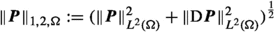
equipped with the norm $\left\| \varvec{P}\right\| _{\sharp }^{2}=\left\| \text {sym}\,\varvec{P}\right\| _{L^2}^{2}+\left\| {\text {D}}\!\varvec{P}\right\| _{L^2}^{2}$ are Hilbert spaces (i.e., we cannot have generalized rigid body motion $\varvec{A}\in \mathfrak {so}(3)$) and that $\left\| \cdot \right\| _{\sharp }^{2}$ is equivalent to $\left\| \cdot \right\| _{1,2,\Omega }^{2}$. The well-posedness of the associated homogeneous problems

$$\begin{aligned} \int _{\Omega }W(\text {D}\varvec{u},\varvec{P},\text {D}\varvec{P})\,\text {d}V\longrightarrow \min ,\qquad \left( \varvec{u},\varvec{P}\right) \in H_{0,\Gamma }^{1}(\Omega ,\mathbb {R}^{3})\times \mathscr {H}_{\text {sym}\,}^{\sharp }\!(\Omega ) \end{aligned}$$

(167)

and

$$\begin{aligned} \int _{\Omega }W(\text {D}\varvec{u},\varvec{P},\text {D}\varvec{P})\,\text {d}V\longrightarrow \min ,\qquad \left( \varvec{u},\varvec{P}\right) \in H_{0,\Gamma }^{1}(\Omega ,\mathbb {R}^{3})\times \mathscr {H}_{\text {dev}\,\text {sym}\,}^{\sharp }\!(\Omega ), \end{aligned}$$

(168)

respectively, follows as before.

References

1. Aivaliotis, A., Daouadji, A., Barbagallo, G., Tallarico, D., Neff, P., Madeo, A.: Microstructure-related Stoneley waves and their effect on the scattering properties of a 2D Cauchy/relaxed-micromorphic interface. Wave Motion 90, 99–120 (2019)
Article  MathSciNet  MATH  Google Scholar
2. Alavi, S., Ganghoffer, J., Reda, H., Sadighi, M.: Construction of micromorphic continua by homogenization based on variational principles. J. Mech. Phys. Solids 153, 104278 (2021)
Article  MathSciNet  Google Scholar
3. Alberdi, R., Robbins, J., Walsh, T., Dingreville, R.: Exploring wave propagation in heterogeneous metastructures using the relaxed micromorphic model. J. Mech. Phys. Solids 155, 104540 (2021)
4. Altenbach, H., Müller, W.H., Abali, B.E.: Higher Gradient Materials and Related Generalized Continua. Springer, Berlin (2019)
Book  Google Scholar
5. Barbagallo, G., Madeo, A., d’Agostino, M.V., Abreu, R., Ghiba, I.-D., Neff, P.: Transparent anisotropy for the relaxed micromorphic model: macroscopic consistency conditions and long wave length asymptotics. Int. J. Solids Struct. 120, 7–30 (2017)
Article  Google Scholar
6. Barbagallo, G., Tallarico, D., d’Agostino, M.V., Aivaliotis, A., Neff, P., Madeo, A.: Relaxed micromorphic model of transient wave propagation in anisotropic band-gap metastructures. Int. J. Solids Struct. 162, 148–163 (2019)
7. Cosserat, E., Cosserat, F.: Théorie des corps déformables (1909)
8. d’Agostino, M.V., Barbagallo, G., Ghiba, I.-D., Abreu, R., Madeo, A., Neff, P.: A panorama of dispersion curves for the isotropic weighted relaxed micromorphic model. Z. Angew. Math. Mech. 97(11), 1436–1481 (2017)
MathSciNet  MATH  Google Scholar
9. d’Agostino, M.V., Barbagallo, G., Ghiba, I.-D., Eidel, B., Neff, P., Madeo, A.: Effective description of anisotropic wave dispersion in mechanical band-gap metamaterials via the relaxed micromorphic model. J. Elast. 139(2), 299–329 (2020)
10. De Cicco, S., Nappa, L.: Torsion and flexure of microstretch elastic circular cylinders. Int. J. Eng. Sci. 35(6), 573–583 (1997)
Article  MATH  Google Scholar
11. dell’Isola, F., Sciarra, G., Vidoli, S.: Generalized Hooke’s law for isotropic second gradient materials. Proc. R. Soc. A: Math. Phys. Eng. Sci. 465(2107), 2177–2196 (2009)
Article  ADS  MathSciNet  MATH  Google Scholar
12. Ebobisse, F., Neff, P.: A fourth-order gauge-invariant gradient plasticity model for polycrystals based on Kröner’s incompatibility tensor. Math. Mech. Solids 25(2), 129–159 (2020)
13. Eremeyev, V., dell-Isola, F.: Weak solutions within the gradient-incomplete strain-gradient elasticity. Lobachevskii J. Math. 41(10), 1992–1998 (2020)
14. Eremeyev, V.A.: On the characterization of the nonlinear reduced micromorphic continuum with the local material symmetry group. In: Higher Gradient Materials and Related Generalized Continua, pp. 43–54. Springer (2019)
15. Eremeyev, V.A., Cazzani, A., dell-Isola, F: On nonlinear dilatational strain gradient elasticity. Continuum Mech. Thermodyn., pp. 1–35 (2021)
16. Eremeyev, V.A., dell-Isola, F.: On weak solutions of the boundary value problem within linear dilatational strain gradient elasticity for polyhedral Lipschitz domains. Math. Mech. Solids, 10812865211025576 (2021)
17. Eremeyev, V.A., et al.: A note on reduced strain gradient elasticity. In: Generalized Models and Non-classical Approaches in Complex Materials 1, pp. 301–310. Springer (2018)
18. Eremeyev, V.A., Lurie, S.A., Solyaev, Y.O., dell-Isola, F.: On the well posedness of static boundary value problem within the linear dilatational strain gradient elasticity. Z. Angew. Math. Phys. 71(6), 1–16 (2020)
19. Eringen, A.C.: Mechanics of micromorphic materials. In: Applied Mechanics, pp. 131–138. Springer, Berlin (1966)
20. Eringen, A.C.: Mechanics of micromorphic continua. In: Mechanics of Generalized Continua, pp. 18–35. Springer (1968)
21. Eringen, A.C., Claus, W.D., Jr.: A micromorphic approach to dislocation theory and its relation to several existing theories. In: Fundamental Aspects of Dislocation Theory, Volume II. National Bureau of Standards Special, 317(2), 1023–1040 (1970)
22. Fantuzzi, N., Leonetti, L., Trovalusci, P., Tornabene, F.: Some novel numerical applications of Cosserat continua. Int. J. Comput. Methods 15(06), 1850054 (2018)
23. Fantuzzi, N., Trovalusci, P., Luciano, R.: Material symmetries in homogenized hexagonal-shaped composites as Cosserat continua. Symmetry 12(3), 441 (2020)
Article  ADS  Google Scholar
24. Forest, S.: Micromorphic media. In: Altenbach, H., Eremeyev, V. (eds.) Generalized Continua from the Theory to Engineering Applications, 541, pp. 249–300. Springer, Berlin (2013)
Chapter  Google Scholar
25. Forest, S.: Micromorphic approach to materials with internal length. In: Encyclopedia of Continuum Mechanics, pp. 1–11. Springer, Berlin (2018)
Google Scholar
26. Ganghoffer, J., Simonsson, K.: A micromechanical model of the martensitic transformation. Mech. Mater. 27(3), 125–144 (1998)
27. Ghiba, I.-D., Neff, P., Madeo, A., Münch, I.: A variant of the linear isotropic indeterminate couple-stress model with symmetric local force-stress, symmetric nonlocal force-stress, symmetric couple-stresses and orthogonal boundary conditions. Math. Mech. Solids 22(6), 1221–1266 (2017)
28. Ghiba, I.-D., Neff, P., Madeo, A., Placidi, L., Rosi, G.: The relaxed linear micromorphic continuum: existence, uniqueness and continuous dependence in dynamics. Math. Mech. Solids 20(10), 1171–1197 (2014)
29. Ghiba, I.-D., Rizzi, G., Madeo, A., Neff, P.: Cosserat micropolar elasticity: classical eringen vs. dislocation form. arXiv preprint arXiv:2206.02473 (2022)
30. Hütter, G.: Homogenization of a Cauchy continuum towards a micromorphic continuum. J. Mech. Phys. Solids 99, 394–408 (2017)
Article  ADS  MathSciNet  Google Scholar
31. Hütter, G.: On the micro-macro relation for the microdeformation in the homogenization towards micromorphic and micropolar continua. J. Mech. Phys. Solids 127, 62–79 (2019)
32. Jeong, J., Neff, P.: Existence, uniqueness and stability in linear Cosserat elasticity for weakest curvature conditions. Math. Mech. Solids 15(1), 78–95 (2010)
33. Jeong, J., Ramézani, H., Münch, I., Neff, P.: A numerical study for linear isotropic Cosserat elasticity with conformally invariant curvature. Z. Angew. Math. Mech. 89(7), 552–569 (2009)
34. Kirchner, N., Steinmann, P.: Mechanics of extended continua: modeling and simulation of elastic microstretch materials. Comput. Mech. 40(4), 651–666 (2007)
35. Lakes, R.: Experimental methods for study of Cosserat elastic solids and other generalized elastic continua. Continuum Models Mater. Microstruct. 70, 1–25 (1995)
MATH  Google Scholar
36. Lakes, R., Drugan, W.: Bending of a Cosserat elastic bar of square cross section: theory and experiment. J. Appl. Mech. 82(9), 091002 (2015)
37. Lewintan, P., Müller, S., Neff, P.: Korn inequalities for incompatible tensor fields in three space dimensions with conformally invariant dislocation energy. Calc. Var. Partial. Differ. Equ. 60(4), 1–46 (2021)
38. Lewintan, P., Neff, P.: \(L^p\)-trace-free generalized Korn inequalities for incompatible tensor fields in three space dimensions. In: Proceedings of the Royal Society of Edinburgh: Section A Mathematics, pp. 1–32 (2021)
39. Lewintan, P., Neff, P.: \(L^p\)-trace-free version of the generalized korn inequality for incompatible tensor fields in arbitrary dimensions. Z. Angew. Math. Phys. 72(3), 1–14 (2021)
40. Lewintan, P., Neff, P.: Nečas-Lions lemma revisited: an \(L^p\)-version of the generalized Korn inequality for incompatible tensor fields. Math. Methods Appl. Sci. (2021)
41. Madeo, A., Ghiba, I.-D., Neff, P., Münch, I.: A new view on boundary conditions in the Grioli–Koiter–Mindlin–Toupin indeterminate couple stress model. Eur. J. Mech.-A/Solids 59, 294–322 (2016)
42. Madeo, A., Neff, P., d’Agostino, M.V., Barbagallo, G.: Complete band gaps including non-local effects occur only in the relaxed micromorphic model. Comptes Rendus Mécanique 344(11), 784–796 (2016)
43. Madeo, A., Neff, P., Ghiba, I.-D., Placidi, L., Rosi, G.: Band gaps in the relaxed linear micromorphic continuum. Z. Angew. Math. Mech. 95(9), 880–887 (2014)
44. Madeo, A., Neff, P., Ghiba, I.-D., Placidi, L., Rosi, G.: Wave propagation in relaxed micromorphic continua: modeling metamaterials with frequency band-gaps. Continuum Mech. Thermodyn. 27(4–5), 551–570 (2015)
45. Madeo, A., Neff, P., Ghiba, I.-D., Rosi, G.: Reflection and transmission of elastic waves in non-local band-gap metamaterials: a comprehensive study via the relaxed micromorphic model. J. Mech. Phys. Solids 95, 441–479 (2016)
46. Mahnken, R., Ju, X.: Goal-oriented adaptivity based on a model hierarchy of mean-field and full-field homogenization methods in linear elasticity. Int. J. Numer. Meth. Eng. 121(2), 277–307 (2020)
47. Mariano, P.M., Modica, G.: Ground states in complex bodies. ESAIM: Control Optim. Calc. Var. 15(02), 377–402 (2009)
48. Mariano, P.M., Stazi, F.L.: Computational aspects of the mechanics of complex materials. Archi. Comput. Methods Eng. 12(4), 391–478 (2005)
49. Masiani, R., Trovalusci, P.: Cosserat and Cauchy materials as continuum models of brick masonry. Meccanica 31(4), 421–432 (1996)
50. Mindlin, R.D.: Micro-structure in linear elasticity. Arch. Ration. Mech. Anal. 16(1), 51–78 (1964)
51. Münch, I., Neff, P., Madeo, A., Ghiba, I.-D.: The modified indeterminate couple stress model: why Yang et al. ’s arguments motivating a symmetric couple stress tensor contain a gap and why the couple stress tensor may be chosen symmetric nevertheless. Z. Angew. Math. Mech. 97(12), 1524–1554 (2017)
52. Neff, P.: On Korn’s first inequality with non-constant coefficients. Proc. R. Soc. Edinb.: Sect. A Math. 132(01), 221 (2002)
53. Neff, P.: The Cosserat couple modulus for continuous solids is zero viz the linearized Cauchy-stress tensor is symmetric. Z. Angew. Math. Mech. 86(11), 892–912 (2006)
54. Neff, P., Eidel, B., d’Agostino, M.V., Madeo, A.: Identification of scale-independent material parameters in the relaxed micromorphic model through model-adapted first order homogenization. J. Elast. 139(2), 269–298 (2020)
55. Neff, P., Ghiba, I.-D., Madeo, A., Placidi, L., Rosi, G.: A unifying perspective: the relaxed linear micromorphic continuum. Continuum Mech. Thermodyn. 26(5), 639–681 (2014)
56. Neff, P., Jeong, J., Fischle, A.: Stable identification of linear isotropic Cosserat parameters: bounded stiffness in bending and torsion implies conformal invariance of curvature. Acta Mech. 211(3–4), 237–249 (2010)
57. Neff, P., Jeong, J., Münch, I., Ramézani, H.: Mean field modeling of isotropic random Cauchy elasticity versus microstretch elasticity. Z. Angew. Math. Phys. 60(3), 479–497 (2009)
58. Neff, P., Jeong, J., Ramézani, H.: Subgrid interaction and micro-randomness: novel invariance requirements in infinitesimal gradient elasticity. Int. J. Solids Struct. 46(25–26), 4261–4276 (2009)
59. Neff, P., Madeo, A., Barbagallo, G., d’Agostino, M.V., Abreu, R., Ghiba, I.-D.: Real wave propagation in the isotropic-relaxed micromorphic model. Proc. R. Soc. A: Math. Phys. Eng. Sci. 473(2197), 20160790 (2017)
60. Neff, P., Münch, I.: Curl bounds Grad on SO(3). ESAIM Control Optim. Calculus Var. 14(1), 148–159 (2008)
61. Neff, P., Pauly, D., Witsch, K.-J.: A canonical extension of Korn’s first inequality to H(Curl) motivated by gradient plasticity with plastic spin. C.R. Math. 349(23), 1251–1254 (2011)
62. Neff, P., Pauly, D., Witsch, K.-J.: Maxwell meets Korn: a new coercive inequality for tensor fields in \({\mathbb{R} }^{N\times \, N}\) with square-integrable exterior derivative. Math. Methods Appl. Sci. 35(1), 65–71 (2012)
63. Neff, P., Pauly, D., Witsch, K.-J.: Poincaré meets Korn via Maxwell: extending Korn’s first inequality to incompatible tensor fields. J. Differ. Equ. 258(4), 1267–1302 (2015)
Article  ADS  MATH  Google Scholar
64. Nye, J.F.: Some geometrical relations in dislocated crystals. Acta Metall. 1(2), 153–162 (1953)
65. Owczarek, S., Ghiba, I.-D., d’Agostino, M.-V., Neff, P.: Nonstandard micro-inertia terms in the relaxed micromorphic model: well-posedness for dynamics. Math. Mech. Solids 24(10), 3200–3215 (2019)
66. Rahali, Y., Eremeyev, V., Ganghoffer, J.-F.: Surface effects of network materials based on strain gradient homogenized media. Math. Mech. Solids 25(2), 389–406 (2020)
67. Reda, H., Alavi, S., Nasimsobhan, M., Ganghoffer, J.: Homogenization towards chiral cosserat continua and applications to enhanced timoshenko beam theories. Mech. Mater. 155, 103728 (2021)
68. Rizzi, G., Dal Corso, F., Veber, D., Bigoni, D.: Identification of second-gradient elastic materials from planar hexagonal lattices. Part II. Mechanical characteristics and model validation. Int. J. Solids Struct. 176, 19–35 (2019)
69. Rizzi, G., Hütter, G., Khan, H., Ghiba, I-D, Madeo, A., Neff, P.: Analytical solution of the cylindrical torsion problem for the relaxed micromorphic continuum and other generalized continua (including full derivations). Math. Mech. Solids (2021)
70. Rizzi, G., Hütter, G., Madeo, A., Neff, P.: Analytical solutions of the cylindrical bending problem for the relaxed micromorphic continuum and other generalized continua. Continuum Mech. Thermodyn., pp. 1–35 (2021)
71. Rizzi, G., Hütter, G., Madeo, A., Neff, P.: Analytical solutions of the simple shear problem for micromorphic models and other generalized continua. Arch. Appl. Mech. 91(5), 2237–2254 (2021)
72. Rizzi, G., Khan, H., Ghiba, I D., Madeo, A., Neff, P.: Analytical solution of the uniaxial extension problem for the relaxed micromorphic continuum and other generalized continua (including full derivations). Arch. Appl. Mech. (2021)
73. Romano, G., Barretta, R., Diaco, M.: Micromorphic continua: non-redundant formulations. Continuum Mech. Thermodyn. (2016)
74. Rueger, Z., Lakes, R.: Strong Cosserat elasticity in a transversely isotropic polymer lattice. Phys. Rev. Lett. 120(6), 065501 (2018)
75. Scalia, A.: Extension, bending and torsion of anisotropic microstretch elastic cylinders. Math. Mech. Solids 5(1), 31–40 (2000)
76. Scherer, J.-M., Phalke, V., Besson, J., Forest, S., Hure, J., Tanguy, B.: Lagrange multiplier based vs micromorphic gradient-enhanced rate-(in) dependent crystal plasticity modelling and simulation. Comput. Methods Appl. Mech. Eng. 372, 113426 (2020)
77. Shaat, M., Ghavanloo, E., Fazelzadeh, SA.: Review on nonlocal continuum mechanics: physics, material applicability, and mathematics. Mech. Mater., 103587 (2020)
78. Taliercio, A.: Torsion of micropolar hollow circular cylinders. Mech. Res. Commun. 37(4), 406–411 (2010)
79. Taliercio, A., Veber, D.: Some problems of linear elasticity for cylinders in micropolar orthotropic material. Int. J. Solids Struct. 46(22–23), 3948–3963 (2009)
80. Trovalusci, P., Augusti, G.: A continuum model with microstructure for materials with flaws and inclusions. Le J. de Phys. IV, 8(PR8), Pr8–383 (1998)
81. Trovalusci, P., De Bellis, M.L., Masiani, R.: A multiscale description of particle composites: from lattice microstructures to micropolar continua. Compos. B Eng. 128, 164–173 (2017)
82. Trovalusci, P., Ostoja-Starzewski, M., De Bellis, M.L., Murrali, A.: Scale-dependent homogenization of random composites as micropolar continua. Eur. J. Mech.-A/Solids 49, 396–407 (2015)
83. Wallen, S.P., Goldsberry, B.M., Haberman, M.R.: Willis coupling in micromorphic elasticity. J. Acoust. Soc. Am. 150(4), A107–A108 (2021)
Download references
Acknowledgements
Angela Madeo acknowledges support from the European Commission through the funding of the ERC Consolidator Grant META-LEGO, N 101001759. Angela Madeo and Gianluca Rizzi acknowledge funding from the French Research Agency ANR, “METASMART” (ANR-17CE08-0006). Angela Madeo and Gianluca Rizzi acknowledge support from IDEXLYON in the framework of the “Programme Investissement d’Avenir’ ANR-16-IDEX-0005. Patrizio Neff acknowledges support in the framework of the DFG-Priority Programme 2256 “Variational Methods for Predicting Complex Phenomena in Engineering Structures and Materials,” funded by the Deutsche Forschungsgemeinschaft (DFG, German research foundation), Project-ID 422730790, and a collaboration of projects ‘Mathematical analysis of microstructure in supercompatible alloys’ (Project-ID 441211072) and‘A variational scale-dependent transition scheme - from Cauchy elasticity to the relaxed micromorphic continuum’ (Project-ID 440935806). Peter Lewintan and Patrizio Neff were supported by the Deutsche Forschungsgemeinschaft (Project-ID 415894848). Hassam Khan acknowledges the support of the German Academic Exchange Service (DAAD) and the Higher Education Commission of Pakistan (HEC).
Author information
Authors and Affiliations
Authors
Corresponding author
Correspondence to Marco Valerio d’Agostino.
Additional information
Communicated by Andreas Öchsner.
Publisher's Note
Springer Nature remains neutral with regard to jurisdictional claims in published maps and institutional affiliations.