
Abstract
Statistics is a fundamental tool to study physical phenomena in any system, be it complex or not. However, it is particularly important in the study of complex systems, for reasons that will be explained in this chapter in detail.
Access this chapter
Tax calculation will be finalised at checkout
Purchases are for personal use only
Notes
- 1.
In the case of the room temperature, a = −273.13∘C and b = +∞; for a component of the fluid velocity, a = −∞; b = +∞ while its magnitude varies between a = 0 and b = +∞. Finally, waiting-times between disintegrations vary within the range defined by a = 0 and b = +∞.
- 2.
We will always represent probabilities with an uppercase P. Also, we will represent the generic outcome of an observation or experiment by an uppercase X.
- 3.
For instance, a Gaussian pdf will exceed 1 if w < 1/(2π). A Cauchy will exceed 1 if γ < 1/π.
- 4.
Both the cdf and the sf are very useful tools to determine the tails of pdfs in the case of power-law statistics, as will be discussed in Sect. 2.4.3.
- 5.
The survival function is also known as the complementary cumulative distribution function (or ccdf). The name survival function originated in biological studies that investigated the probability of a certain species surviving beyond a certain length of time.
- 6.
The error function used in Table 2.2 is defined as:
$$\displaystyle \begin{aligned} \mathrm{erf}(x)\equiv \frac{2}{\sqrt{\pi}}\int_0^x dx~e^{-x^2}.\end{aligned} $$(2.8)Table 2.2 Cumulative distribution and survival functions of some common pdfs - 7.
Characteristic functions are very important in the context of complex systems since, for many meaningful pdfs with power-law tails, only their characteristic function has a closed analytical expression. This makes, for instance, that comparisons against experimental data can often be done more easily using the characteristic function.
- 8.
The mean should not be confused with the most probable value, that is that value of x where p(x) reaches its maximum. It is also different from the median, that is the value x m , for which P(X > x m ) = P(X < x m ).
- 9.
The standard deviation is often used to estimate the error of a measurement, with the mean of all tries providing the estimate for the measurement. In this case, it is implicitly assume that all errors are accidental, devoid of any bias [5].
- 10.
Note that our definition of kurtosis corresponds to what in some textbooks is called the excess kurtosis. In those cases, the kurtosis is defined instead as \(\kappa := \left \langle (x-\mu )^4\right \rangle /c_2^2\) which, for a Gaussian pdf yields a value of three. The excess kurtosis is then defined as κ e := κ − 3, so that a positive κ e means a heavier tail than a Gaussian and a negative value, the opposite.
- 11.
The skewness and kurtosis are particularly useful to detect departures of Gaussian behaviour in experimental data, due to the fact that the cumulants of the Gaussian pdf satisfy that c n = 0, n > 2 (see Problem 2.4). These deviations are also referred to as deviations of normality, since the Gaussian is also known as the normal distribution!
- 12.
One must however remain cautious and avoid taking any of these general ideas as indisputable evidence. Such connections, although often meaningful, are not bullet-proof and sometimes even completely wrong. Instances exist of complex systems that exhibit Gaussian statistics, and non-complex systems with power-law statistics. It is thus advisable to apply as many additional diagnostics as possible in order to confirm or disregard what might emerge from the statistical analysis of the system. Knowing as much as possible about the underlying physics also helps.
- 13.
A random variable is the way we refer to the unpredictable outcome of an experiment or measurement. Mathematically, it is possible to give a more precise definition, but in practical terms, its unpredictability is its more essential feature.
- 14.
For example, Gaussian distributions are also well suited to model unbiased measurement errors, since they are always assumed to be the result of many additive, independent factors [5].
- 15.
s > 1 is needed to make sure that the pdf be integrable and normalizable to unity. We also assume x > 0, but the same argument could be done for x < 0 by changing x →−x.
- 16.
We adhere to the convention of representing the Gaussian with the uppercase letter N, a consequence of its being called the normal distribution.
- 17.
For that reason, CLT states that the average of random variables with individual pdfs exhibiting tails p(x) ∼ x −s will be attracted towards a Lévy distribution with α = s − 1 if s < 3. The value of λ of the attractor distribution will depend on the level of asymmetry of the individual pdfs.
- 18.
The case of maximum asymmetry (i.e., when |λ| = 1) is particularly interesting, and will be discussed separately later in this chapter. We will also refer to it often in Chap. 5, while discussing fractional transport in the context of continuous time random walks.
- 19.
Although the name Lévy distribution is used, in this book, for any member of the Lévy family of pdfs, in many statistical contexts the name is reserved to this specific choice of parameters. This is kind of unfortunate, and can lead to confusions sometimes.
- 20.
For α > 1, the Lévy pdfs with λ = ±1 do cover the whole real line, but it can be shown that they vanish exponentially fast as x →∓∞ [7].
- 21.
In fact, some authors include the Gaussian as the only non-divergent member of the Lévy family.
- 22.
These reasons may include, for instance, the varying strength of the immune system of the people encountered, their personal resistance to that particular contagion, the specific weather of that day or whether the day of interest is a working day or part of a weekend.
- 23.
We have normalized \(N^{k+1}_{\text{infected}}\) to the initial number infected for simplicity.
- 24.
In many cases, extreme events have such a long-term influence on the system that, in spite of their apparently small probability, they dominate the system dynamics. One could think, for instance, of the large earthquakes that happen in the Earth’s crust, or of the global economical crisis that affect the world economy, and the impact that may have on our daily life for many years after.
- 25.
A related pdf, the Laplace pdf, can be defined for both positive and negative values:
$$\displaystyle \begin{aligned} \mathrm{Lp}_{\tau}(x) = \frac{1}{2\tau} \exp(-|x|/\tau),~~~~\varOmega =(-\infty,\infty). \end{aligned} $$(2.60)However, the Laplace pdf does not play any similar role to the exponential in regards to time processes. It is somewhat reminiscent of the Gaussian distribution, although it decays quite more slowly as revealed by its larger kurtosis value (see Table 2.4).
- 26.
One must be careful, though. There are examples of complex systems with exponential statistics. For instance, a randomly-driven running sandpile exhibits exponential statistics for the waiting-times between avalanches. This is a consequence of the fact that avalanches are triggered only when a grain of sand drops, which happens randomly throughout the sandpile. It is only when sufficiently large avalanches are considered that non-exponential waiting-time statistics become apparent, revealing the true complex behaviour of the sandpile, as we will see in Sect. 4.5.
- 27.
This follows from the fact that the triggering of events in a Poisson process is independent of the past history of the process. Thus, what we may have already waited for is irrelevant and cannot condition how much more we will have to wait for the next triggering!
- 28.
The conditional probability of B happening assuming that A has already happened, P(A|B), is given by: P(A|B) = P(A ∩ B)/P(A), where P(A ∩ B) is the joint probability of events A and B happening, and P(A) is the probability of A happening [4].
- 29.
Indeed, note that due to the properties of the exponential function, it follows that:
$$\displaystyle \begin{aligned} P[ W \geq w + \hat w]= \exp(a(w+\hat w) ) = \exp(aw )\cdot\exp(a \hat w) = P[ W \geq \hat w] \cdot P[ W\geq \hat w]. \end{aligned} $$(2.63) - 30.
Discrete means that the possible outcomes are countable; in this case, the number of events k, that can only take integer values. One consequence of being discrete is that the distribution gives actual probabilities, so that it is no longer a density of probability.
- 31.
Note that the Poisson distribution is a discrete distribution, not a pdf, and is normalized to unity only when summing over all possible values of k. Can the reader prove this?
- 32.
Remember that Γ(x) becomes the usual factorial function, Γ(k + 1) = k!, for integer k.
- 33.
This is, in fact, a nice example of a physical system in which the appearance of a power law in a pdf has nothing to do with any complex behaviour, and the exponential decay at large t is not a finite size effect.
- 34.
It was first introduced by R. Kohlrausch to describe the discharge of a capacitor at the end of the nineteenth century, and is often used in the context of relaxation processes.
- 35.
This idea is rooted in the perceived prevalence of Gaussian pdfs, whose cumulants higher than the variance all vanish.
- 36.
It is worth to point out the relation between these prescriptions, that we all learned in high school, and Eqs. 2.24 and 2.25, that require knowledge of the full pdf. Given a series of data \(\left \{ x_i, ~i=1, 2, \cdots N\right \}\), these prescriptions for the mean and variance are given by:
$$\displaystyle \begin{aligned} \bar x := \frac{1}{N} \sum_{i=1}^N x_i,~~~\sigma^2 := \frac{1}{N} \sum_{i=1}^N x^2_i - \bar x^2. \end{aligned} $$(2.74)It is simple to show that the same formulas are obtained if one introduces the numerical pdf obtained from the data series in Eqs. 2.24 and 2.25. Let’s take the mean. The sum over all data points that appears in its definition can be rewritten as a sum over all possible different values of x, if we multiply each value by the number of times it appears. Since the sum is normalized to N, the total number of data points, the sum over all different possible values would become just a sum of the products of each value and its probability. That is, precisely, what Eqs. 2.24 and 2.25 express. Can the reader prove the same equivalence for the variance?
- 37.
The central values are also the ones that contribute more strongly to the values of means and moments, except in cases in which these moments diverge!
- 38.
For Gaussian-distributed data, it must be said that both methods work pretty well.
- 39.
CBS tends to give flatter tails because, in most bins out there, there is either one point or no point at all. Since one only plots the bins with non-zero values, the tail seems artificially flatter than it actually is.
- 40.
These methods will in fact yield a very noisy pdf, since numerical derivatives magnify errors!
- 41.
To build the cumulative distribution function, cdf(x), the procedure is identical to the one discussed here for the survival function, but the initial reordering of the data should be in increasing order!
- 42.
Or the cumulative distribution function method, if one is interested in estimating the tail for negative values of the outcome.
- 43.
Indeed, remember that p(A ∪ B) = p(A)p(B) + p(A ∩ B). Thus, the probability of A and B happening equals the product of their individual probabilities only if events A and B are independent.
- 44.
The likelihood is not the same as the probability, since it is a product of probabilities densities, not of probabilities. That is, one would need to multiply each \(p(X_i|\,p_1,\cdots ,p_ {N_e})\) by dX i to get a probability. In fact, the likelihood is related to the joint pdf of the data set. That is, the probability of each of the values being between X i and X i + dX i simultaneously.
- 45.
It is because of this type of substitution that maximum likelihood estimators are said to be biased and some authors prefer other approaches [13]. This is a consequence of the fact that, in general, the estimator for a function of some parameter is usually not exactly identical to the evaluation of the function at the estimator for that parameter. Or, in other words, that \(\hat f(x) \neq f(\hat x)\).
- 46.
Power-laws are often (but not always!) related to complex dynamics (see Chap. 3).
- 47.
Usually, one needs to use some numerical algorithm to search for zeros of nonlinear equations. For instance, a Newton method [18].
- 48.
- 49.
- 50.
Γ x (a) is the incomplete gamma function, that is defined as:
$$\displaystyle \begin{aligned} \varGamma_x(a) = \int_0^x ds ~ s^{a-1}e^{-s}.\end{aligned} $$(2.116)Fig. 2.17 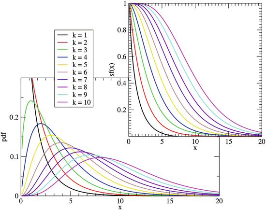
Left box: Chi-square distribution for the first integer k indices; on the right, its survival function, sf(x) = P[X ≥ x] (see Eq. 2.6)
- 51.
In contrast, systematic errors have a non-zero mean, introducing a bias in the quantity being measured.
- 52.
The number of independent values, also known as the number of degrees of freedom, is given by the number of data points N minus the number of parameters that define the model pdf, N e .
- 53.
There are many publicly available packages that do it. For instance, the popular statistical package R is one of them.
- 54.
Similar tables can be easily found in the literature. See, for instance, [21].
- 55.
The longest avalanches in the absence of overlapping will be of the order of the system size, since propagation from one cell to the next takes one iteration.
- 56.
Although note that the transport of sand in the sandpile always happens down the slope!
- 57.
This association certainly becomes more obscure when avalanches overlap either in space and time. Can the reader explain why? This is the reason for choosing the running sandpile parameters so carefully. In particular, N b and p 0.
- 58.
We adopt here a convention for the Fourier transform that is common in the fields of probability and random processes, from which many results will be referred to in Chaps. 3–5. This convention has the benefit of converting the characteristic function into the Fourier transform of the pdf (see Sect. 2.2.4). In other contexts, however, the positive exponential is often reserved for the inverse transform, with the negative exponential used in the direct transform. Regarding normalization, it is also common to find texts that use 2πıkx in the exponent of the exponentials (instead of just ıkx), so that the 1/2π prefactor of the inverse transform disappears. In other cases, the exponent is kept without the 2π factor, but both direct or inverse transforms have a \(1/\sqrt {2\pi }\) prefactor.
- 59.
We will always represent the Fourier transform with a hat symbol, \(\hat f\). Whenever the real variable represents a time, t, the wave number is referred to as a frequency, and represented as ω.
- 60.
The name power spectrum was made popular in the context of turbulence, where f usually represents a velocity or velocity increment. The power spectrum then roughly quantifies the “amount of energy” contained between k and k + dk. For that reason, this theorem is often interpreted in Physics as a statement of the conservation of energy. In other context, the interpretation may vary. In information theory, for instance, Parseval’s theorem represents the conservation of information.
- 61.
It should be noted that |x|−a with 0 < a < 1 is an example of a function that is not Lebesgue integrable and has a Fourier transform. Its Fourier transform, \(\hat f(k) = \varGamma (1-a)k^{a-1}\), however diverges for k → 0 as a result.
- 62.
Most programming languages provide with intrinsic functions to generate series of data with a uniform distribution u ∈ [0.1]. Thus, we will not explain how to do it here!
- 63.
This inverse is known as the quantile function in statistics.
- 64.
The double factorial is defined as n!! = n(n − 2)(n − 4)⋯.

References
Taylor, G.I.: The Spectrum of Turbulence. Proc. R. Soc. Lond. 164, 476 (1938)
Balescu, R.: Equilibrium and Non-equilibrium Statistical Mechanics. Wiley, New York (1974)
Tijms, H.: Understanding Probability. Cambridge University Press, Cambridge (2002)
Feller, W.: An Introduction to Probability Theory and Its Applications. Wiley, New York (1968)
Taylor, J.R.: An Introduction to Error Analysis: The Study of Uncertainties in Physical Measurements. University Science Books, New York (1996)
Gnedenko, B.V., Kolmogorov, A.N.: Limit Distributions for Sums of Independent Random Variables. Addison-Wesley, New York (1954)
Samorodnitsky, G., Taqqu, M.S.: Stable Non-Gaussian Processes. Chapman & Hall, New York (1994)
Aitchison, J., Brown, J.A.C.: The Log-Normal Distribution. Cambridge University Press, Cambridge (1957)
Carr, P., Wu, L.: The Finite Moment Log-Stable Process and Option Pricing. J. Financ. 53, 753 (2003)
Kida, S.: Log-Stable Distribution in Turbulence. Fluid Dyn. Res. 8, 135 (1993)
Kotz, S., Nadarajah, S.: Extreme Value Distributions: Theory and Applications. Imperial College Press, London (2000)
Cox, D.R., Isham, V.: Point Processes. Chapman & Hall, New York (1980)
Mood, A., Graybill, F.A., Boes, D.C.: Introduction to the Theory of Statistics. McGraw-Hill, New York (1974)
Chakravarti, I.M., Laha, R.G., Roy, J.: Handbook of Methods of Applied Statistics. Wiley, New York (1967)
Jaynes, E.T.: Probability Theory: The Logic of Science. Cambridge University Press, Cambridge (2003)
Aldrich, J.: R. A. Fisher and the Making of Maximum Likelihood (1912–1922). Stat. Sci. 12, 162 (1997)
Clauset, A., Shalizi, C.R., Newman, M.E.J.: Power-Law Distributions in Empirical Data. SIAM Rev. 51, 661 (2009)
Press, W.H., Teukolsky, S.A., Vetterling, W.T., Flannery, B.P.: Numerical Recipes in Fortran 90. Cambridge University Press, Cambridge (1996)
Brorsen, B.W., Yang, S.R.: Maximum Likelihood Estimates of Symmetric Stable Distribution Parameters. Commun. Stat. 19, 1459 (1990); Nolan, J.: Levy Processes, Chap. 3. Springer, Heidelberg (2001)
Stephens, M.A.: EDF Statistics for Goodness of Fit and Some Comparisons. J. Am. Stat. Assoc. 69, 730 (1974)
Abramowitz, M., Stegun, I.A.: Handbook of Mathematical Functions. National Bureau of Standards, Washington, DC (1970)
Hwa, T., Kardar, M.: Avalanches, Hydrodynamics and Discharge Events in Models of Sandpile. Phys. Rev. A 45, 7002 (1992)
Bracewell, R.N.: The Fourier Transform and Its Applications. McGraw-Hill, Boston (2000)
Chambers, J.M., Mallows, C.L., Stucka, B.W.: Method for Simulating Stable Random Variables. J. Am. Stat. Assoc. 71, 340 (1976)
Weron, R.: On the Chambers-Mallows-Stuck Method for Simulating Skewed Stable Random Variables. Stat. Probab. Lett. 28, 165 (1996)
Forbes, C., Evans, M., Hastings, M., Peacock B.: Statistical Distributions. Wiley, New York (2010)
Author information
Authors and Affiliations
Appendices
Appendix 1: The Fourier Transform
The Fourier representation has a very large number of applications in Mathematics, Physics and Engineering, since it permits to express an arbitrary function as a linear combination of periodic functions. Truncation of the Fourier representation, for example, is the basis of signal filtering. Many other manipulations (modulation, integration, etc.) form the basis of modern communications. In Physics, use of the Fourier representation is essential for the understanding of resonances, oscillations, wave propagation, transmission and absorption, fluid and plasma turbulence and many other processes. In Mathematics, Fourier transforms are often used to simplify the solution of differential equations, among many other problems.
The Fourier transform of a (maybe complex) function f(x) is defined asFootnote 58:
where \(\i = \sqrt {-1}\), k is known as the wave number.Footnote 59 Note that, if f(x) is real, then \(\hat f(k)\) is Hermitian, meaning that \(\hat f(-k) = \hat f^*(k)\), where the asterisk represents the complex conjugate.
The inverse of the Fourier transform is then obtained as,
This expression is also referred to as the Fourier representation of f(x).
Some common Fourier transform pairs are collected in Table 2.7. However, it must be noted that the existence of both the Fourier and inverse transforms is not always guaranteed. A sufficient condition (but not necessary) is that both f(x) and \(\hat f(k)\) be (Lebesgue)-integrable. That is,
which requires that | f(x)|→ 0 faster than |x|−1 for x →±∞, and that \(|\,\hat f(k)|\rightarrow 0\) faster than |k|−1 for k →±∞. But Fourier transforms may exist for some functions that violate this condition.
Fourier transforms have many interesting properties. In particular, they are linear operations. That is, the Fourier transform of the sum of any two functions is equal to the sum of their Fourier transforms.
Secondly, the Fourier transform of the n -th derivative of a function becomes particularly simple:
as trivially follows from differentiating Eq. 2.124.
Another interesting property has to do with the translation of the argument, that translates into a multiplication by a phase in Fourier space:
Particularly useful properties are the following two theorems [23]. One is Parseval’s theorem,
where the asterisk denotes complex conjugation. When f = g, this becomes,
\(|\,\hat f(k)|{ }^2\) is usually known as the power spectrum of f(x).Footnote 60
The second important theorem is the convolution theorem. It states that the convolution of two functions, defined as:
satisfies that its Fourier transform is given by:
assuming that the individual Fourier transforms, \(\hat f(k)\) and \(\hat g(k)\) do exist.
In the context of scale-invariance, it is useful to note that:
Similarly, the Fourier transform of a power law (see Table 2.7) is also very useful. In particular, it can be shown that, the Fourier transform of f(x) = |x|−a, with 0 < a < 1, is given by another power-law.Footnote 61 Namely,
being Γ(x) Euler’s gamma function. Furthermore, it can be shown that if a function f(x) ∼|x|−a with 0 < a < 1 for x →∞, then its Fourier transform \(\hat f(k) \sim k^{a-1}\) for k → 0.
Appendix 2: Numerical Generation of Series with Prescribed Statistics
One of the most commonly used method generate time series with a prescribed set of statistics is the inverse function method. It is based on passing a time series u whose values follow a uniform distributionFootnote 62 in [0, 1] through an invertible function. That is, we generate a collection of values using:
The series of values for x is then distributed according to the pdf:
To prove this statement, let’s consider the cumulative distribution function associated with p(x) (Eq. 2.4) at x = a, that verifies:
The fourth step follows from the fact that the cumulative function being an increasing function of its argument. The last step is due to the fact that the cumulative distribution function of the uniform distribution is simply its argument! If F(x) = cdf(x), then Eq.2.135 follows after invoking Eq. 2.5.
Generating time series with prescribed statistics is thus reduced to knowing the inverse of the cumulative distribution function of the desired distribution.Footnote 63 For instance, in the case of the exponential pdf, \(E_\tau (x) = \tau ^{-1}\exp (-x/\tau )\), the sought inverse is,
Thus, one can generate a series distributed with an exponential pdf of mean value τ by iterating:
using uniformly-distributed u ∈ [0, 1].
Regretfully, many important distributions do not have analytical expressions for their cdfs. Much less of their inverse! This is the case, for instance, of the Gamma pdf (Eq. 2.70). Another important example is the Lévy distributions, that only have an analytic expression for their characteristic function (Eq. 2.32). Thus, the inverse function method is useless to generate this kind of data. Luckily, a formula exists, based on combining two series of random numbers, u distributed uniformly in [−π/2, π/2], and v distributed exponentially with unit mean, that is able to generate a series of l values distributed according to prescribed Lévy statistics. For α ≠ 1 the formula reads [24, 25]:
with \(K_{\alpha , \lambda } = \tan ^{-1} \left ( \lambda \tan \left (\pi \alpha /2\right )\right )\). For the case α = 1, one should use instead [25]:
These formulas reduce to much simpler expressions in some cases. For instance, in the Gaussian case (α = 2, λ = 0), Eq. 2.139 reduces to:
whilst for the Cauchy distribution (α = 1, λ = 0), Eq. 2.140 reduces to:
Problems
2.1 Survival and Cumulative Distribution Functions
Calculate explicitly the cumulative distribution function and the survival function of the Cauchy, Laplace and exponential pdfs.
2.2 Characteristic Function
Calculate explicitly the characteristic function of the Gaussian, exponential and the uniform pdfs.
2.3 Cumulants and Moments
Derive the relations between cumulants and moments up to order n = 5.
2.4 Gaussian Distribution
Footnote 64Show that for a Gaussian pdf, \(N_{[0,\sigma ^2]}(x)\), all cumulants are zero except for c 2 = σ 2. Also, show that only the even moments are non-zero and equal to m n = σ n(n − 1)!!.
2.5 Log-Normal Distribution
Calculate the first four cumulants of the log-normal distribution defined by Eq. 2.45. Show that they are given by: \(c_1 = \exp (\mu +\sigma ^2/2)\); \(c_2 = (\exp (\sigma ^2) -1 )\exp (2\mu +\sigma ^2)\); \(S = (\exp (\sigma ^2) + 2)\sqrt {\exp (\sigma ^2) - 1}\) and \(K = \exp (4\sigma ^2) +2\exp (3\sigma ^2) + 3\exp (2\sigma ^2) - 6\).
2.6 Poisson Distribution
Derive the limit of the binomial distribution B(k, n;p) for n →∞ and p → 0, keeping np = λ, and prove that it is the Poisson discrete distribution (Eq. 2.67).
2.7 Ergodicity
Consider the process defined by \(y(t) = \cos (\omega t + \phi )\), where ω (the frequency) is fixed, but with a different values of ϕ (the phase) for each realization of the process. Under what conditions are the temporal and ensemble views of the statistics of y equivalent? Or, in other words, when does the process behave ergodically?
2.8 Numerical Estimation of pdfs
Write a code that, given a set of experimental data, \(\left \{x_i, ~~i= 1, 2, \cdots N \right \}\), calculates their pdf using each of the methods described in this chapter: the CBS, CBC and the survival/cumulative distribution function methods.
2.9 Maximum Likelihood Estimators (I)
Calculate the maximum likelihood estimators of the Exponential pdf (Eq. 2.59) and the bounded power-law pdf (Eq. 2.111) using the methodology described in Sect. 2.5.
2.10 Maximum Likelihood Estimators (II)
Prove that, in the case of the Gumbel distribution (Eq. 2.51), the determination of the maximum likelihood estimators for μ and σ requires to solve numerically the pair of coupled nonlinear equations [26]:
Write a numerical code that solves this equation using a nonlinear Newton method [18].
2.11 Synthetic Data Generation
Write a code that implements Eq. 2.139 to generate Lévy distributed synthetic data with arbitrary parameters. Use it to generate at least three different sets of data, and assess the goodness of Eq. 2.139 by computing their pdf.
2.12 Running Sandpile: Sandpile Statistics
Write a code that, given a flip time-series generated by the running sandpile code built in Problem 1.5, is capable of extracting the size and duration of the avalanches contained in it, as well as the waiting-times between them. Use the code proposed in Problem 2.8 to obtain the pdfs of each of these quantities.
2.13 Advanced Problem: Minimum Chi-Square Parameter Estimation
Write a code that, given \(\left \{x_i, ~~i= 1, 2, \cdots N \right \}\), calculates the characteristic function of its pdf, ϕ data(k j ), with k j being the collocation points in Fourier space. Then, estimate the parameters of the Lévy pdf that best reproduces the data by minimizing the target function, \(\chi _k^2(\alpha ,\lambda ,\mu ,\sigma )\), that quantifies the difference between the characteristic function of the data and that of the Lévy pdf (Eq. 2.32):
To minimize \(\chi ^2_k\), the reader should look for any open-source subroutine that can do local optimization. We recommend using, for example, the Levenberg-Marquardt algorithm [18].
Rights and permissions
Copyright information
© 2018 Springer Science+Business Media B.V.
About this chapter

Cite this chapter
Sánchez, R., Newman, D. (2018). Statistics. In: A Primer on Complex Systems. Lecture Notes in Physics, vol 943. Springer, Dordrecht. https://doi.org/10.1007/978-94-024-1229-1_2
Download citation
DOI: https://doi.org/10.1007/978-94-024-1229-1_2
Published:
Publisher Name: Springer, Dordrecht
Print ISBN: 978-94-024-1227-7
Online ISBN: 978-94-024-1229-1
eBook Packages: Physics and AstronomyPhysics and Astronomy (R0)