Proofs of Work From Worst-Case Assumptions

Abstract

We give Proofs of Work (PoWs) whose hardness is based on well-studied worst-case assumptions from fine-grained complexity theory. This extends the work of (Ball et al., STOC ’17), that presents PoWs that are based on the Orthogonal Vectors, 3SUM, and All-Pairs Shortest Path problems. These, however, were presented as a ‘proof of concept’ of provably secure PoWs and did not fully meet the requirements of a conventional PoW: namely, it was not shown that multiple proofs could not be generated faster than generating each individually. We use the considerable algebraic structure of these PoWs to prove that this non-amortizability of multiple proofs does in fact hold and further show that the PoWs’ structure can be exploited in ways previous heuristic PoWs could not.

This creates full PoWs that are provably hard from worst-case assumptions (previously, PoWs were either only based on heuristic assumptions or on much stronger cryptographic assumptions (Bitansky et al., ITCS ’16)) while still retaining significant structure to enable extra properties of our PoWs. Namely, we show that the PoWs of (Ball et al., STOC ’17) can be modified to have much faster verification time, can be proved in zero knowledge, and more.

Finally, as our PoWs are based on evaluating low-degree polynomials originating from average-case fine-grained complexity, we prove an average-case direct sum theorem for the problem of evaluating these polynomials, which may be of independent interest. For our context, this implies the required non-amortizability of our PoWs.

1 Introduction

Proofs of Work (PoWs), introduced in [DN92], have shown themselves to be an invaluable cryptographic primitive. Originally introduced to combat Denial of Service attacks and email spam, their key notion now serves as the heart of most modern cryptocurrencies (when combined with additional desired properties for this application).

By quickly generating easily verifiable challenges that require some quantifiable amount of work, PoWs ensure that adversaries attempting to swarm a system must have a large amount of computational power to do so. Practical uses aside, PoWs at their core ask a foundational question of the nature of hardness: Can you prove that a certain amount of work t was completed? In the context of complexity theory for this theoretical question, it suffices to obtain a computational problem whose (moderately) hard instances are easy to sample such that solutions are quickly verifiable.

Unfortunately, implementations of PoWs in practice stray from this theoretical question and, as a consequence, have two main drawbacks. First, they are often based on heuristic assumptions that have no quantifiable guarantees. One commonly used PoW is the problem of simply finding a value s so that hashing it together with the given challenge (e.g. with SHA-256) maps to anything with a certain amount of leading 0’s. This is based on the heuristic belief that SHA-256 seems to behave unpredictably with no provable guarantees.

Secondly, since these PoWs are not provably secure, their heuristic sense of security stems from, say, SHA-256 not having much discernible structure to exploit. This lack of structure, while hopefully giving the PoW its heuristic security, limits the ability to use the PoW in richer ways. That is, heuristic PoWs do not seem to come with a structure to support any useful properties beyond the basic definition of PoWs.

This work, building on the techniques and the proof of concept of our results in [BRSV17a], addresses both of these problems by constructing PoWs that are based on worst-case complexity theoretic assumptions in a provable way while also having considerable algebraic structure. This simultaneously moves PoWs in the direction of modern cryptography by basing our primitives on well-studied worst-case problems and expands the usability of PoWs by exploiting our algebraic structure to create, for example, PoWs that can be proved in Zero Knowledge or that can be distributed across many workers in a way that is robust to Byzantine failures. Our biggest use of our problems’ structure is in proving a direct sum theorem to show that our proofs are non-amortizable across many challenges; this was the missing piece of [BRSV17a] in achieving PoWs according to their usual definition [DN92].

1.1 On Security From Worst-Case Assumptions

We make a point here that if SHA-256 is secure then it can be made into the aforementioned PoW whereas, if it is not, then SHA-256 is broken. While tautological, we point out that this is a Win-Lose situation. That is, either we have a PoW, or a specific instantiation of a heuristic cryptographic hash function is broken and no new knowledge is gained.

This is in contrast to our provably secure PoWs, in which we either have a PoW, or we have a breakthrough in complexity theory. For example, if we base a PoW on the Orthogonal Vectors problem which we define in Sect. 1.2, then either we have a PoW or the Orthogonal Vectors problem can be solved in sub-quadratic time which has been shown [Wil05] to be sufficient to break the Strong Exponential Time Hypothesis (${\mathsf {SETH}}$), giving a faster-than-brute-force algorithm for CNF-SAT formulas and thus a major insight to the vs problem.

By basing our PoWs on well-studied complexity theoretic problems, we position our conditional results to be in the desirable position for cryptography and complexity theory: a Win-Win. Orthogonal Vectors, 3SUM, and All-Pairs Shortest Path are the central problems of fine-grained complexity theory precisely because of their many quantitative connections to many other computational problems and so breaking any of their associated conjectures would give considerable insight into computation. Heuristic PoWs like SHA-256, however, aren’t even known to have natural generalizations or asymptotics much less connections to other computational problems and so a break would simply say that that specific design for that specific input size happened to not be as secure as we thought.

1.2 Our Results

In this paper we introduce PoWs based on the Orthogonal Vectors (), 3SUM, and All-Pairs Shortest Path problems, which comprise the central problems of the field of fine-grained complexity theory. Similar PoWs were introduced in [BRSV17a], although these failed to prove non-amortizability of these PoWs – that many challenges take proportionally more work, as is required by the definition of PoWs [DN92, BGJ+16]. We show here that the PoWs of [BRSV17a] can be extended to exploit their considerable algebraic structure to show non-amortizability via a direct sum theorem and, thus, that they are genuine PoWs according to the conventional definition. Further, we show that this structure to can be used to allow for much quicker verification and zero-knowledge PoWs. We also note that our structure plugs into the framework of [BK16b] to obtain distributed PoWs robust to Byzantine failure.

While all of our results and techniques will be analogous for and , we will use as our running example for our proofs and results statements. Namely, (defined in Sect. 2.2) is a well-studied problem that is conjectured to require $n^{2-o(1)}$ time in the worst-case [Wil15]. Roughly, we show the following.

Informal Theorem

Suppose takes $n^{2-o(1)}$ time to decide for sufficiently large n. A challenge $\varvec{c}$ can be generated in $\widetilde{O}(n)$ time such that:

• A valid proof $\varvec{\pi }$ to $\varvec{c}$ can be computed in $\widetilde{O}(n^2)$ time.

• The validity of a candidate proof to $\varvec{c}$ can be verified in $\widetilde{O}(n)$ time.

• Any valid proof to $\varvec{c}$ requires $n^{2-o(1)}$ time to compute.

This can be scaled to $n^{k-o(1)}$ hardness for all $k\in \mathbb {N}$ by a natural generalization of the problem to the problem, whose hardness is also supported by ${\mathsf {SETH}}$. Thus fine-grained complexity theory props up PoWs of any complexity that is desired.

Further, we show that the verification can still be done in $\widetilde{O}(n)$ time for all of our $n^{k-o(1)}$ hard PoWs, allowing us to tune hardness. The corresponding PoW for this is interactive but we show how to remove this interaction in the Random Oracle model in Sect. 5.

We also note that a straightforward application of [BK16b] allows our PoWs to be distributed amongst many workers in a way that is robust to byzantine failure or errors and can detect malicious party members. Namely, that a challenge can be broken up amongst a group of provers so that partial work can be error-corrected into a full proof.

Further, our PoWs admit zero knowledge proofs such that the proofs can be simulated in very low complexity – i.e. in time comparable to the verification time. While heuristic PoWs can be proved in zero knowledge as they are statements, the exact polynomial time complexities matter in this regime. We are able to use the algebraic structure of our problem to attain a notion of zero knowledge that makes sense in the fine-grained world.

A main lemma which may be of independent interest is a direct sum theorem on evaluating a specific low-degree polynomial .

Informal Theorem

Suppose takes $n^{k-o(1)}$ time to decide. Then, for any polynomial $\ell$, any algorithm that computes ’s correctly on $\ell$ uniformly random $x_{i}$’s with probability $1/n^{O(1)}$ takes time $\ell (n)\cdot n^{k-o(1)}$.

1.3 Related Work

As mentioned earlier, PoWs were introduced by Dwork and Naor [DN92]. Definitions similar to ours were studied by Jakobsson and Juels [JJ99], Bitansky et al. [BGJ+16], and (under the name Strong Client Puzzles) Stebila et al. [SKR+11] (also see the last paper for some candidate constructions and further references).

We note that, while PoWs are often used in cryptocurrencies, the literature studying them in that context have more properties than the standard notion of a PoW (e.g. [BK16a]) that are desirable for their specific use within cryptocurrency and blockchain frameworks. We do not consider these and instead focus on the foundational cryptographic primitive that is a PoW.

In this paper we build on the work of [BRSV17a], which introduced PoWs whose hardness is based on the same worst-case assumptions we consider here. While [BRSV17a] introduced the PoWs as a proof-of-concept that PoWs can be based on well-studied worst-case assumptions, they did not fully satisfy the definition of a PoW in that the PoWs were not shown to be non-amortizable. That is, it was not proven that many challenges could not be batch-evaluated faster than solving each of them individually. We show here that these PoWs are in fact non-amortizable by proving a direct sum theorem in Sect. 4. Further, the -based PoWs of [BRSV17a] have verification times of $\widetilde{O}(n^{k/2})$ whereas we show how to achieve verification in time $\widetilde{O}(n)$, which makes the PoWs much more realistic for use. These are both properties that are expected of a PoW that were not included in [BRSV17a]. Beyond that, we show that our PoWs can be proved in zero knowledge and note that our PoWs can be distributed across many worker in way that is robust to Byzantine error, both of which are properties seemingly not achievable from the current ‘structureless’ heuristic PoWs that are used.

Provably secure PoWs have been considered before in [BGJ+16] where PoWs are achieved from cryptographic assumptions (even stronger than an average-case assumption). Namely, they show that if there is a worst-case hard problem that is non-amortizable and succinct randomized encodings exist, then PoWs are achievable. In contrast, our PoWs are based on solely on worst-case assumptions on well-studied problems from fine-grained complexity theory.

Subsequent to our work, Goldreich and Rothblum [GR18] have constructed (implicitly) a PoW protocol based on the worst-case hardness of the problem of counting t-cliques in a graph (for some constant t); they show a worst-case to average-case reduction for this problem, a doubly efficient interactive proof, and that the average-case problem is somewhat non-amortizable, which are the properties needed to go from worst-case hardness to PoWs.

A previous version of this paper appeared under the title Proofs of Useful Work [BRSV17b], where we had presented the same protocol as in this paper as a PoW scheme where the prover’s work could be made “useful” by using it to perform independently useful computation. However, it was pointed out to us (by anonymous reviewers) that a naive construction satisfied our definition of a “Useful PoW.”

2 Proofs of Work from Worst-Case Assumptions

In this section, we first define Proof of Work (PoW) schemes, and then present our construction of such a scheme based on the hardness of Orthogonal Vectors () and related problems. In Sect. 2.1, we define PoWs; in Sect. 2.2, we introduce and related problems; in Sect. 2.3, we describe an interactive proof for these problems that is used in our eventual construction, which is presented in Sect. 2.4. Our PoWs, while similar, will differ from those of [BRSV17a] in that we allow interaction to significantly speed the verification time by exploiting the PoWs’ algebraic structure. We will show how to remove interaction in the Random Oracle model in Sect. 5.

2.1 Definition

Syntactically, a Proof of Work scheme involves three algorithms:

• $\mathsf {Gen}(1^{n})$ produces a challenge $\varvec{c}$.

• $\mathsf {Solve}(\varvec{c})$ solves the challenge $\varvec{c}$, producing a proof $\varvec{\pi }$.

• $\mathsf {Verify}(\varvec{c}, \varvec{\pi })$ verifies the proof $\varvec{\pi }$ to the challenge $\varvec{c}$.

Taken together, these algorithms should result in an efficient proof system whose proofs are hard to find. This is formalized as follows.

Definition 2.1

(Proof of Work). A $(t(n), \delta (n))$ -Proof of Work (PoW) consists of three algorithms $(\mathsf {Gen},\mathsf {Solve},\mathsf {Verify})$. These algorithms must satisfy the following properties for large enough n:

• Efficiency:

  • $\mathsf {Gen}(1^{n})$ runs in time $\widetilde{O}(n)$.

  • For any $\varvec{c}\leftarrow \mathsf {Gen}(1^{n})$, $\mathsf {Solve}(\varvec{c})$ runs in time $\widetilde{O}(t(n))$.

  • For any $\varvec{c}\leftarrow \mathsf {Gen}(1^{n})$ and any $\varvec{\pi }$, $\mathsf {Verify}(\varvec{c},\varvec{\pi })$ runs in time $\widetilde{O}(n)$.

• Completeness: For any $\varvec{c}\leftarrow \mathsf {Gen}(1^{n})$ and any $\varvec{\pi }\leftarrow \mathsf {Solve}(\varvec{c})$,

  $$\begin{aligned} \Pr \left[ \mathsf {Verify}(\varvec{c},\varvec{\pi })=accept \right] = 1 \end{aligned}$$

  where the probability is taken over $\mathsf {Verify}$’s randomness.

• Hardness: For any polynomial $\ell$, any constant $\epsilon > 0$, and any algorithm $\mathsf {Solve}^*_\ell$ that runs in time $\ell (n)\cdot t(n)^{1-\epsilon }$ when given $\ell (n)$ challenges of size n as input,

  $$\begin{aligned} \Pr \left[ \forall i: \mathsf {Verify}(\varvec{c}_i,\varvec{\pi }_i) = \text{ acc }\ \left| \begin{array}{l} (\varvec{c}_i \leftarrow \mathsf {Gen}(1^{n}))_{i\in [\ell (n)]} \\ \varvec{\pi }\leftarrow \mathsf {Solve}^*_\ell (\varvec{c}_1, \dots , \varvec{c}_{\ell (n)}):\\ \varvec{\pi }= (\varvec{\pi }_1, \dots ,\varvec{\pi }_{\ell (n)}) \end{array} \right. \right] < \delta (n) \end{aligned}$$

  where the probability is taken over $\mathsf {Gen}$ and $\mathsf {Verify}$’s randomness.

The efficiency requirement above guarantees that the verifier in the Proof of Work scheme runs in nearly linear time. Together with the completeness requirement, it also ensures that a prover who actually spends roughly t(n) time can convince the verifier that it has done so. The hardness requirement says that any attempt to convince the verifier without actually spending the prescribed amount of work has only a small probability of succeeding, and that this remains true even when amortized over several instances. That is, even a prover who gets to see several independent challenges and respond to them together will be unable to reuse any work across the challenges, and is effectively forced to spend the sum of the prescribed amount of work on all of them.

In some of the PoWs we construct, $\mathsf {Solve}$ and $\mathsf {Verify}$ are not algorithms, but are instead parties in an interactive protocol. The requirements of such interactive PoWs are the natural generalizations of those in the definition above, with $\mathsf {Verify}$ deciding whether to accept after interacting with $\mathsf {Solve}$. And the hardness requirement applies to the numerous interactive protocols being run in any form of composition – serial, parallel, or otherwise. We will, however, show how to remove interaction in Sect. 5.

Heuristic constructions of PoWs, such as those based on SHA-256, easily satisfy efficiency and completeness (although not formally, given their lack of asymptotics), yet their hardness guarantees are based on nothing but the heuristic assumption that the PoW itself is a valid PoW. We will now reduce the hardness of our PoW to the hardness of well-studied worst-case problems in fine-grained complexity theory.

2.2 Orthogonal Vectors

We now formally define the problems – Orthogonal Vectors () and its generalization – whose hardness we use to construct our PoW scheme. The properties possessed by that enable this construction are also shared by other well-studied problems mentioned earlier, including and as noted in [BRSV17a], and an array of other problems [BK16b, GR17, Wil16]. Consequently, while we focus on , PoWs based on the hardness of these other problems can be constructed along the lines of the one here. Further, the security of these constructions would also follow from the hardness of other problems that reduce to , , etc. in a fine-grained manner with little, if any, degradation of security. Of particular interest, deciding graph properties that are statable in first-order logic all reduce to (moderate-dimensional) [GI16], and so we can obtain PoWs if any problem statable as a first-order graph property is hard.

All the algorithms we consider henceforth – reductions, adversaries, etc. – are non-uniform Word-RAM algorithms (with words of size $O(\log {n})$ where n will be clear from context) unless stated otherwise, both in our hardness assumptions and our constructions. Security against such adversaries is necessary for PoWs to remain hard in the presence of pre-processing, which is typical in the case of cyrptocurrencies, for instance, where specialized hardware is often used. In the case of reductions, this non-uniformity is solely used to ensure that specific parameters determined completely by instance size (such as the prime p(n) in Definition 2.5) are known to the reductions.

Remark 2.2

All of our reductions, algorithms, and assumptions can easily be made uniform by having an extra procedure that is allowed to run in $t(n)^{1-\epsilon }$ for some $\epsilon >0$ for a $(t(n),\delta (n))$-PoW. In our setting, this will just be used to find a prime on which to base a field extension for the rest of the PoW to satisfy the rest of its conditions. This makes sense for a PoW scheme to do and, for all the problems we consider, this can be done be done so that all the conjectures can be made uniformly. We leave everything non-uniform, however, for exposition’s sake.

Definition 2.3

(Orthogonal Vectors). The problem on vectors of dimension d (denoted ) is to determine, given two sets U, V of n vectors from $\left\{ 0,1 \right\} ^{d(n)}$ each, whether there exist $u\in U$ and $v\in V$ such that $\langle u,v \rangle = 0$ (over $\mathbb {Z}$). If left unspecified, d is to be taken to be $\left\lceil \log ^2n \right\rceil$.

is commonly conjectured to require $n^{2-o(1)}$ time to decide, for which many conditional fine-grained hardness results are based on [Wil15], and has been shown to be true if the Strong Exponential Time Hypothesis (${\mathsf {SETH}}$) holds [Wil05]. This hardness and the hardness of its generalization to of requiring $n^{k-o(1)}$ time (which also holds under ${\mathsf {SETH}}$) are what we base the hardness of our PoWs on. We now define .

Definition 2.4

(k-Orthogonal Vectors). For an integer $k \ge 2$, the problem on vectors of dimension d is to determine, given k sets $(U_1, \dots , U_k)$ of n vectors from $\left\{ 0,1 \right\} ^{d(n)}$ each, whether there exist $u^s\in U_s$ for each $s \in [k]$ such that over $\mathbb {Z}$,

$$\begin{aligned} \sum _{\ell \in [d(n)]} u^1_{\ell } \cdots u^k_{\ell } = 0 \end{aligned}$$

We say that such a set of vectors is k-orthogonal. If left unspecified, d is to be taken to be $\left\lceil \log ^2n \right\rceil$.

While these problems are conjectured worst-case hard, there are currently no widely-held beliefs for distributions that it may be average-case hard over. [BRSV17a], however, defines a related problem that is shown to be average-case hard when assuming the worst-case hardness of . This problem is that of evaluating the following polynomial:

For any prime number p, we define the polynomial as follows. Its inputs are parsed in the manner that those of are: below, for any $s \in [k]$ and $i \in [n]$, $u^s_i$ represents the $i^{\text {th}}$ vector in $U_s$, and for $\ell \in [d]$, $u^s_{i\ell }$ represents its $\ell ^{\text {th}}$ coordinate.

When given an instance of (from $\left\{ 0,1 \right\} ^{knd}$) as input, counts the number of tuples of k-orthogonal vectors (modulo p). Note that the degree of this polynomial is kd; for small d (e.g. $d=\left\lceil \log ^2n \right\rceil$), this is a fairly low-degree polynomial. The following definition gives the family of such polynomials parameterized by input size.

Definition 2.5

( ). Consider an integer $k \ge 2$. Let p(n) be the smallest prime number larger than $n^{\log {n}}$, and $d(n) = \left\lceil \log ^2{n} \right\rceil$. is the family of functions .

Remark 2.6

We note that most of our results would hold for a much smaller choice of p(n) above – anything larger than $n^k$ would do. The reason we choose p to be this large is to achieve negligible soundness error in interactive protocols we shall be designing for this family of functions (see Protocol 1.1). Another way to achieve this is to use large enough extension fields of $\mathbb {F}_p$ for smaller p’s; this is actually preferable, as the value of p(n) as defined now is much harder to compute for uniform algorithms.

2.3 Preliminaries

Our final protocol and its security consists, essentially, of two components – the hardness of evaluating on random inputs, and the the ability to certify the correct evaluation of in an efficiently verifiable manner. We explain the former in the next subsection; here, we describe the protocol for the latter (Protocol 1.1), which we will use as a sub-routine in our final PoW protocol. This protocol is a $(k-1)$-round interactive proof that, given $U_1, \dots , U_k \in \mathbb {F}_p^{nd}$ and $y \in \mathbb {F}_p$, proves that .

In the special case of $k=2$, a non-interactive () protocol for was shown in [Wil16] and this protocol was used to construct a PoW scheme based on , , and in [BRSV17a], albeit one that only satisfies a weaker hardness requirement (i.e. non-batchability was not considered or proved). We introduce interaction to greatly improve the verifier’s efficiency and show how interaction can be removed in Sect. 5. The following interactive proof is essentially the sum-check protocol, but in our case we need to pay close attention to the complexity of the prover and the verifier and so use ideas from [Wil16].

We will set up the following definitions before describing the protocol. For each $s \in [k]$, consider the univariate polynomials $\phi ^s_1, \dots , \phi ^s_d: \mathbb {F}_p \rightarrow \mathbb {F}_p$, where $\phi ^s_\ell$ represents the $\ell ^{\text {th}}$ column of $U_s$ – that is, for $i\in [n]$, $\phi ^s_\ell (i) = u^s_{i\ell }$. Each $\phi ^s_\ell$ has degree at most $(n-1)$. can now be written as:

where q is defined for convenience as:

$$\begin{aligned} q(i_1, \dots , i_k) = \prod _{\ell \in [d]} \left( 1 - \phi ^1_\ell (i_1) \cdots \phi ^k_{\ell }(i_k) \right) \end{aligned}$$

The degree of q is at most $D = k(n-1)d$. Note that q can be evaluated at any point in $\mathbb {F}_p^k$ in time $\widetilde{O}(knd\log {p})$, by evaluating all the $\phi ^s_\ell (i_s)$’s (these polynomials can be found using fast interpolation techniques for univariate polynomials [Hor72]), computing each term in the above product and then multiplying them.

For any $s \in [k]$ and $\alpha _1, \dots , \alpha _{s-1} \in \mathbb {F}_p$, define the following univariate polynomial:

$$\begin{aligned} q_{s,\alpha _1, \dots , \alpha _{s-1}} (x) = \sum _{i_{s+1}, \dots , i_k \in [n]} q(\alpha _1, \dots , \alpha _{s-1}, x, i_{s+1}, \dots , i_k) \end{aligned}$$

Every such $q_s$ has degree at most $(n-1)d$ – this can be seen by inspecting the definition of q. With these definitions, the interactive proof is described as Protocol 1.1 below. The completeness and soundness of this interactive proof is then asserted by Theorem 2.7, which is proven in Sect. 3.

Theorem 2.7

For any $k \ge 2$, let d and p be as in Definition 2.5. Protocol 1.1 is a $(k-1)$-round interactive proof for proving that . This protocol has perfect completeness and soundness error at most $\left( \frac{knd}{p}\right)$. The prover runs in time $\widetilde{O}(n^kd\log {p})$, and the verifier in time $\widetilde{O}(knd^2\log {p})$.

As observed earlier, Protocol 1.1 is non-interactive when $k=2$. We then get the following corollary for .

Corollary 2.8

For $k = 2$, let d and p be as in Definition 2.5. Protocol 1.1 is an proof for proving that . This protocol has perfect completeness and soundness error at most $\left( \frac{2nd}{p}\right)$. The prover runs in time $\widetilde{O}(n^2)$, and the verifier in time $\widetilde{O}(n)$.

2.4 The PoW Protocol

We now present Protocol 1.2, which we show to be a Proof of Work scheme assuming the hardness of .

Theorem 2.9

For some $k \ge 2$, suppose takes $n^{k-o(1)}$ time to decide for all but finitely many input lengths for any $d = \omega (\log {n})$. Then, Protocol 1.2 is an $(n^k,\delta )$-Proof of Work scheme for any function $\delta (n) > 1/n^{o(1)}$.

Remark 2.10

As is, this will be an interactive Proof of Work protocol. In the special case of $k=2$, Corollary 2.8 gives us a non-interactive PoW. If we want to remove interaction for general , however, we could use the proof in [Wil16] at the cost of verification taking time $\widetilde{O}(n^{k/2})$ as was done in [BRSV17a]. To keep verification time at $\widetilde{O}(n)$, we instead show how to remove interaction in the Random Oracle model in Sect. 5. This will allow us to tune the gap between the parties – we can choose k and thus the amount of work, $n^{k-o(1)}$, that must be done by the prover while always only needing $\widetilde{O}(n)$ time for verification.

Remark 2.11

We can also exploit this PoW’s algebraic structure on the Prover’s side. Using techniques from [BK16b], the Prover’s work can be distributed amongst a group of provers. While, cumulatively, they must complete the work required of the PoW, they can each only do a portion of it. Further, this can be done in a way robust to Byzantine errors amongst the group. See Remark 3.4 for further details.

We will use Theorem 2.7 to argue for the completeness and soundness of Protocol 1.2. In order to prove the hardness, we will need lower bounds on how well the problem that $\mathsf {Solve}$ is required to solve can be batched. We first define what it means for a function to be non-batchable in the average-case in a manner compatible with the hardness requirement. Note that this requirement is stronger than being non-batchable in the worst-case.

Definition 2.12

Consider a function family $\mathcal {F}= \left\{ f_n:\mathcal {X}_n\rightarrow \mathcal {Y}_n \right\}$, and a family of distributions $\mathcal {D}= \left\{ D_n \right\}$, where $D_n$ is over $\mathcal {X}_n$. $\mathcal {F}$ is not $(\ell ,t,\delta )$-batchable on average over $\mathcal {D}$ if, for any algorithm $\mathsf {Batch}$ that runs in time $\ell (n)t(n)$ when run on $\ell (n)$ inputs from $\mathcal {X}_n$, when it is given as input $\ell (n)$ independent samples from $D_n$, the following is true for all large enough n:

We will be concerned with the case where the batched time t(n) is less than the time it takes to compute $f_n$ on a single instance. This sort of statement is what a direct sum theorem for $\mathcal {F}$’s hardness would guarantee. Theorem 2.13, then, claims that we achieve this non-batchability for and, as is one of the things that $\mathsf {Solve}$ is required to evaluate, we will be able to show the desired hardness of Protocol 1.2. We prove Theorem 2.13 via a direct sum theorem in Appendix A, and prove a weaker version for illustrative purposes in Sect. 4.

Theorem 2.13

For some $k \ge 2$, suppose takes $n^{k-o(1)}$ time to decide for all but finitely many input lengths for any $d = \omega (\log {n})$. Then, for any constants $c,\epsilon > 0$ and $\delta < \epsilon /2$, is not $(n^c,n^{k-\epsilon },1/n^{\delta })$-batchable on average over the uniform distribution over its inputs.

We now put all the above together to prove Theorem 2.9 as follows.

Proof of Theorem 2.9. We prove that Protocol 1.2 satisfies the various requirements demanded of a Proof of Work scheme assuming the hardness of .

Efficiency:

• $\mathsf {Gen}(1^n)$ simply samples knd uniformly random elements of $\mathbb {F}_p$. As $d = \log ^2{n}$ and $p \le 2n^{\log {n}}$ (by Bertrand-Chebyshev’s Theorem), this takes $\widetilde{O}(n)$ time.

• $\mathsf {Solve}$ computes , which can be done in $\widetilde{O}(n^k)$ time. It then runs the prover in an instance of Protocol 1.1, which can be done in $\widetilde{O}(n^k)$ time by Theorem 2.7. So in all it takes takes $\widetilde{O}(n^k)$ time.

• $\mathsf {Verify}$ runs the verifier in an instance of Protocol 1.1, taking $\widetilde{O}(n)$ time, again by Theorem 2.7.

Completeness: This follows immediately from the completeness of Protocol 1.1 as an interactive proof for , as stated in Theorem 2.7, as this is the protocol that $\mathsf {Solve}$ and $\mathsf {Verify}$ engage in.

Hardness: We proceed by contradiction. Suppose there is a polynomial $\ell$, an (interactive) algorithm $\mathsf {Solve}^*$, and a constant $\epsilon > 0$ such that $\mathsf {Solve}^*$ runs in time $\ell (n) n^{k-\epsilon }$ and makes $\mathsf {Verify}$ accept on $\ell (n)$ independent challenges generated by $\mathsf {Gen}(1^n)$ with probability at least $\delta (n) > 1/n^{o(1)}$ for infinitely many input lengths n.

For each of these input lengths, let the set of challenges (which are inputs) produced by $\mathsf {Gen}(1^n)$ be $\left\{ \varvec{c}_1,\dots ,\varvec{c}_{\ell (n)} \right\}$, and the corresponding set of solutions output by $\mathsf {Solve}^*$ be $\left\{ z_1,\dots ,z_{\ell (n)} \right\}$. So $\mathsf {Solve}^*$ succeeds as a prover in Protocol 1.1 for all the instances $\left\{ (\varvec{c}_i,z_i) \right\}$ with probability at least $\delta (n)$.

By the negligible soundness error of Protocol 1.1 guaranteed by Theorem 2.7, in order to do this, $\mathsf {Solve}^*$ has to use the correct values for all the $z_i$’s with probability negligibly close to $\delta (n)$ and definitely more than, say, $\delta (n)/2$. In particular, with this probability, it has to explicitly compute at $\varvec{c}_1, \dots , \varvec{c}_{\ell (n)}$, all of which are independent uniform points in $\mathbb {F}_p^{knd}$ for all of these infinitely many input lengths n. But this is exactly what Theorem 2.13 says is impossible under our assumptions. So such a $\mathsf {Solve}^*$ cannot exist, and this proves the hardness of Protocol 1.2.

We have thus proven all the properties necessary and hence Protocol 1.2 is indeed an $(n^k,\delta )$-Proof of Work under the hypothesised hardness of for any $\delta (n) > 1/n^{o(1)}$.    $\square$

3 Verifying

In this section, we prove Theorem 2.7 (stated in Sect. 2), which is about Protocol 1.1 being a valid interactive proof for proving evaluations of . We use here terminology from the theorem statement and protocol description. Recall the the input to the protocol is $U_1, \dots , U_k \in \mathbb {F}_p^{nd}$ and $y\in \mathbb {F}_p$, and the prover wishes to prove that .

Completeness. If indeed , the prover can make the verifier in the protocol accept by using the polynomials $(q_1, q_{2,\alpha _1}, \dots , q_{k,\alpha _1, \dots , \alpha _k})$ in place of $(q^*_1, q^*_{2,\alpha _1}, \dots , q^*_{k,\alpha _1, \dots , \alpha _k})$. Perfect completeness is then seen to follow from the definitions of these polynomials and their relation to q and hence .

Soundness. Suppose . We now analyze the probability with which a cheating prover could make the verifier accept.

To start with, note that the prover’s $q_1^*$ has to be different from $q_1$, as otherwise the check in the second step would fail. Further, as the degree of these polynomials is less than nd, the probability that the verifier will then choose an $\alpha _1$ such that $q_1^*(\alpha _1) = q_1(\alpha _1)$ is less than $\frac{nd}{p}$.

If this event does not happen, then the prover has to again send a $q_{2,\alpha _1}^*$ that is different from $q_{2,\alpha _1}$, which again agree on $\alpha _2$ with probability less than $\frac{nd}{p}$. This goes on for $(k-1)$ rounds, at the end of which the verifier checks whether $q_{k-1}^*(\alpha _{k-1})$ is equal to $q_{k-1}(\alpha _{k-1})$, which it computes by itself. If at least one of these accidental equalities at a random point has not occurred throughout the protocol, the verifier will reject. The probability that no violations occur over the $(k-1)$ rounds is, by the union bound, less than $\frac{knd}{p}$.

Efficiency. Next we discuss details of how the honest prover and the verifier are implemented, and analyze their complexities. To this end, we will need the following algorithmic results about computations involving univariate polynomials over finite fields.

Lemma 3.1

(Fast Multi-point Evaluation [Fid72]). Given the coefficients of a univariate polynomial $q:\mathbb {F}_p \rightarrow \mathbb {F}_p$ of degree at most N, and N points $x_1, \dots , x_N \in \mathbb {F}_p$, the set of evaluations $(q(x_1), \dots , q(x_N))$ can be computed in time $O(N\log ^3{N}\log {p})$.

Lemma 3.2

(Fast Interpolation [Hor72]). Given $N+1$ evaluations of a univariate polynomial $q: \mathbb {F}_p \rightarrow \mathbb {F}_p$ of degree at most N, the coefficients of q can be computed in time $O(N\log ^3{N}\log {p})$.

To start with, both the prover and verifier compute the coefficients of all the $\phi ^s_\ell$’s. Note that, by definition, they know the evaluation of each $\phi ^s_\ell$ on n points, given by $\left\{ (i,u^s_{i\ell }) \right\} _{i\in [n]}$. This can be used to compute the coefficients of each $\phi ^s_\ell$ in time $\widetilde{O}(n\log {p})$ by Lemma 3.2. The total time taken is hence $\widetilde{O}(knd\log {p})$.

The proof of the following proposition specifies further details of the prover’s workings.

Proposition 3.3

The coefficients of the polynomial $q_{s,\alpha _1, \dots , \alpha _{s-1}}$ can be computed in time $\widetilde{O}((n^{k-s+1}d + nd^2)\log {p})$ given the above preprocessing.

Proof

The procedure to do the above is as follows:

• 1. Fix some value of $s, \alpha _1, \dots , \alpha _{s-1}$.

• 2. For each $\ell \in [d]$, compute the evaluation of $\phi ^s_\ell$ on nd points, say $\left\{ 1, \dots , nd \right\}$.

  • Since its coefficients are known, the evaluations of each $\phi ^s_\ell$ on these nd points can be computed in time $\widetilde{O}(nd\log {p})$ by Lemma 3.1, for a total of $\widetilde{O}(nd^2\log {p})$ for all the $\phi ^s_\ell$’s.

• 3. For each setting of $i_{s+1}, \dots , i_k$, compute the evaluations of the polynomial $\rho _{i_{s+1}, \dots , i_k}(x) = q(\alpha _1, \dots , \alpha _{s-1}, x, i_{s+1}, \dots , i_k)$, on the points $\left\{ 1, \dots , nd \right\}$.

  • First substitute the constants $\alpha _1, \dots , \alpha _{s-1}, i_{s+1}, \dots , i_k$ into the definition of q.

  • This requires computing, for each $\ell \in [d]$ and $s' \in [k]\setminus \left\{ s \right\}$, either $\phi ^{s'}_\ell (\alpha _s)$ or $\phi ^{s'}_\ell (i_s)$. All of this can be done in time $\widetilde{O}(knd\log {p})$ by direct polynomial evaluations since the coefficients of the $\phi ^{s'}_\ell$’s are known.

  • This reduces q to a product of d univariate polynomials of degree less than n, whose evaluations on the nd points can now be computed in time $\widetilde{O}(knd\log {p})$ by multiplying the constants computed in the above step with the evaluations of $\phi ^{s'}_\ell$ on these points, and subtracting from 1.

  • The product of the evaluations can now be computed in time $\widetilde{O}(nd^2\log {p})$ to get what we need.

• 4. Add up the evaluations of $\rho _{i_{s+1}, \dots , i_k}$ pointwise over all settings of $(i_{s+1}, \dots , i_k)$.

  • There are $n^{k-s}$ possible settings of $(i_{s+1}, \dots , i_k)$, and for each of these we have nd evaluations. All the additions hence take $\widetilde{O}(n^{k-s+1}d\log {p})$ time.

• 5. This gives us nd evaluations of $q_{s,\alpha _1, \dots , \alpha _{s-1}}$, which is a univariate polynomial of degree at most $(n-1)d$. So its coefficients can be computed in time $\widetilde{O}(nd\log {p})$ by Lemma 3.2.

It can be verified from the intermediate complexity computations above that all these operations together take $\widetilde{O}((n^{k-s+1}d+nd^2)\log {p})$ time. This proves the proposition.    $\square$

Recall that what the honest prover has to do is compute $q_1, q_{2,\alpha _1}, \dots ,$ $q_{k,\alpha _1, \dots , \alpha _{k-1}}$ for the $\alpha _s$’s specified by the verifier. By the above proposition, along with the preprocessing, the total time the prover takes is:

$$\begin{aligned} \widetilde{O}(knd\log {p} + (n^{k}d+nd^2)\log {p}) = \widetilde{O}(n^{k}d\log {p}) \end{aligned}$$

The verifier’s checks in steps (2) and (3) can each be done in $\widetilde{O}(n\log {p})$ time using Lemma 3.1. Step (4), finally, can be done by using the above proposition with $s = k$ in time $\widetilde{O}(nd^2\log {p})$. Even along with the preprocessing, this leads to a total time of $\widetilde{O}(knd^2\log {p})$.

Remark 3.4

Note the Prover’s work of finding coefficients of polynomials is mainly done by evaluating the polynomial on many points and interpolating. Similarly to [BK16b], this opens the door to distributing the Prover’s work. Namely, the individual evaluations can be split amongst a group of workers which can then be recombined to find the final coefficients. Further, since the evaluations of a polynomial is a Reed-Solomon code, this allows for error correction in the case that the group of provers make errors or have some malicious members. Thus, the Prover’s work can be distributed in a way that is robust to Byzantine errors and can identify misbehaving members.

4 A Direct Sum Theorem for

A direct sum theorem for a problem roughly states that solving m independent instances of a problem takes m times as long as a single instance. The converse of this is attaining a non-trivial speed-up when given a batch of instances. In this section we prove a direct sum theorem for the problem of evaluating and thus its non-batchability.

Direct sum are typically elusive in complexity theory and so our results, which we prove for generic problems with a certain set of properties, may be of independent interest to the study of hardness amplification. That our results show that batch-evaluating our multivariate low-degree polynomials is hard may be particularly surprising since batch-evaluation for univariate low-degree polynomials is known to be easy [Fid72, Hor72] and, further, [BK16b, GR17, Wil16] show that batch-evaluating multivariate low-degree polynomials (including our own) is easy to delegate. For more rigorous definitions of direct sum and direct product theorems, see [She12].

We now prove the following weaker version of Theorem 2.13 on ’s non-batchability (Theorem 2.13 is proven in Appendix A using an extension of the techniques employed here). The notion of non-batchability used below is defined in Definition 2.12 in Sect. 2.

Theorem 4.1

For some $k \ge 2$, suppose takes $n^{k-o(1)}$ time to decide for all but finitely many input lengths for any $d = \omega (\log {n})$. Then, for any constants $c,\epsilon > 0$, is not $(n^c,n^{k-\epsilon },7/8)$-batchable on average over the uniform distribution over its inputs.

Throughout this section, $\mathcal {F}$, $\mathcal {F}'$ and $\mathcal {G}$ are families of functions $\left\{ f_n : \mathcal {X}_n \rightarrow \mathcal {Y}_n \right\}$, $\left\{ f'_n : \mathcal {X}'_n \rightarrow \mathcal {Y}'_n \right\}$ and $\left\{ g_n : \hat{\mathcal {X}}_n \rightarrow \hat{\mathcal {Y}}_n \right\}$, and $\mathcal {D}= \left\{ D_n \right\}$ is a family of distributions where $D_n$ is over $\hat{\mathcal {X}}_n$.

Theorem 4.1 is the result of two properties possessed by . We define these properties below, prove a more general lemma about functions that have these properties, and use it to prove this theorem.

Definition 4.2

$\mathcal {F}$ is said to be $(s,\ell )$-downward reducible to $\mathcal {F}'$ in time t if there is a pair of algorithms $(\mathsf {Split},\mathsf {Merge})$ satisfying:

• For all large enough n, $s(n) < n$.

• $\mathsf {Split}$ on input an $x \in \mathcal {X}_n$ outputs $\ell (n)$ instances from $\mathcal {X}'_{s(n)}$.

  $$\begin{aligned} \mathsf {Split}(x) = (x_1, \dots , x_{\ell (n)}) \end{aligned}$$

• Given the value of $\mathcal {F}'$ at these $\ell (n)$ instances, $\mathsf {Merge}$ can reconstruct the value of $\mathcal {F}$ at x.

  $$\begin{aligned} \mathsf {Merge}(x, f'_{s(n)}(x_1), \dots , f'_{s(n)}(x_{\ell (n)})) = f_n(x) \end{aligned}$$

• $\mathsf {Split}$ and $\mathsf {Merge}$ together run in time at most t(n).

If $\mathcal {F}'$ is the same as $\mathcal {F}$, then $\mathcal {F}$ is said to be downward self-reducible.

Definition 4.3

$\mathcal {F}$ is said to be $\ell$-robustly reducible to $\mathcal {G}$ in time t if there is a pair of algorithms $(\mathsf {Split},\mathsf {Merge})$ satisfying:

• $\mathsf {Split}$ on input an $x \in \mathcal {X}_n$ (and randomness r) outputs $\ell (n)$ instances from $\hat{\mathcal {X}}_{n}$.

  $$\begin{aligned} \mathsf {Split}(x;r) = (x_1, \dots , x_{\ell (n)}) \end{aligned}$$

• For such a tuple $(x_i)_{i\in [\ell (n)]}$ and any function $g^*$ such that $g^*(x_i) = g_n(x_i)$ for at least $2{\text {/}}3$ of the $x_i$’s, $\mathsf {Merge}$ can reconstruct the function value at x as:

  $$\begin{aligned} \mathsf {Merge}(x,r,g^*(x_1), \dots , g^*(x_{\ell (n)})) = f_n(x) \end{aligned}$$

• $\mathsf {Split}$ and $\mathsf {Merge}$ together run in time at most t(n).

• Each $x_i$ is distributed according to $D_n$, and the $x_i$’s are pairwise independent.

The above is a more stringent notion than the related non-adaptive random self-reducibility as defined in [FF93]. We remark that to prove what we need, it can be shown that it would have been sufficient if the reconstruction above had only worked for most r’s.

Lemma 4.4

Suppose $\mathcal {F}$, $\mathcal {F}'$ and $\mathcal {G}$ have the following properties:

• $\mathcal {F}$ is $(s_d,\ell _d)$-downward reducible to $\mathcal {F}'$ in time $t_d$.

• $\mathcal {F}'$ is $\ell _r$-robustly reducible to $\mathcal {G}$ over $\mathcal {D}$ in time $t_r$.

• $\mathcal {G}$ is $(\ell _a,t_a,7/8)$-batchable on average over $\mathcal {D}$, and $\ell _a(s_d(n)) = \ell _d(n)$.

Then $\mathcal {F}$ can be computed in the worst-case in time:

$$\begin{aligned} t_d(n) + \ell _d(n) t_r(s_d(n)) + \ell _r(s_d(n)) \ell _d(n) t_a(s_d(n)) \end{aligned}$$

We note, that the condition $\ell _a(s_d(n)) = \ell _d(n)$ above can be relaxed to $\ell _a(s_d(n)) \le \ell _d(n)$ at the expense of a factor of 2 in the worst-case running time obtained for $\mathcal {F}$. We now show how to prove Theorem 4.1 using Lemma 4.4, and then prove the lemma itself.

Proof of Theorem 4.1. Fix any $k \ge 2$. Suppose, towards a contradiction, that for some $c, \epsilon > 0$, is $(n^c,n^{k-\epsilon },7/8)$-batchable on average over the uniform distribution. In our arguments we will refer to the following function families:

• $\mathcal {F}$ is with vectors of dimension $d = \left( \frac{k}{k+c}\right) ^2 \log ^2{n}$.

• $\mathcal {F}'$ is with vectors of dimension $\log ^2{n}$.

• $\mathcal {G}$ is (over $\mathbb {F}_p^{knd}$ for some p that definitely satisfies $p > n$).

Let $m = n^{k/(k+c)}$. Note the following two properties :

• $\frac{n}{m^{c/k}} = m$

• $d = \left( \frac{k}{k+c}\right) ^2 \log ^2{n} = \log ^2{m}$

We now establish the following relationships among the above function families.

Proposition 4.5

$\mathcal {F}$ is $\left( m, m^c\right)$-downward reducible to $\mathcal {F}'$ in time $\widetilde{O}(m^{c+1})$.

$\mathsf {Split}_d$, when given an instance $(U_1, \dots , U_k) \in \left\{ 0,1 \right\} ^{k(n\times d)}$, first divides each $U_i$ into $m^{c/k}$ partitions $U_{i1}, \dots , U_{im^{c/k}} \in \left\{ 0,1 \right\} ^{m \times d}$. It then outputs the set of tuples $\left\{ (U_{1j_1}, \dots , U_{kj_k})\ |\ j_i \in [m^{c/k}] \right\}$. Each $U_{ij}$ is in $\left\{ 0,1 \right\} ^{m\times d}$ and, as noted earlier, $d = \log ^2{m}$. So each tuple in the set is indeed an instance of $\mathcal {F}'$ of size m. Further, there are $(m^{c/k})^c = m^c$ of these.

Note that the original instance has a set of k-orthogonal vectors if and only if at least one of the $m^c$ smaller instances produced does. So $\mathsf {Merge}_d$ simply computes the disjunction of the $\mathcal {F}'$ outputs to these instances.

Both of these can be done in time $O(m^c\cdot k\cdot md + m^c) = \widetilde{O}(m^{c+1})$.

Proposition 4.6

$\mathcal {F}'$ is 12kd-robustly reducible to $\mathcal {G}$ over the uniform distribution in time $\widetilde{O}(m)$.

Notice that for any $U_1, \dots , U_k \in \left\{ 0,1 \right\} ^{m\times d}$, we have that . So it is sufficient to show such a robust reduction from $\mathcal {G}$ to itself. We do this now.

Given input $\varvec{x}\in \mathbb {F}_p^{knd}$, $\mathsf {Split}_r$ picks two uniformly random $\varvec{x}_1, \varvec{x}_2 \in \mathbb {F}_p^{knd}$ and outputs the set of vectors $\left\{ \varvec{x}+t\varvec{x}_1+t^2\varvec{x}_2\ |\ t \in \left\{ 1, \dots , 12kd \right\} \right\}$. Recall that our choice of p is much larger than 12kd and hence this is possible. The distribution of each of these vectors is uniform over $\mathbb {F}_p^{knd}$, and they are also pairwise independent as they are points on a random quadratic curve through $\varvec{x}$.

Define the univariate polynomial . Note that its degree is at most 2kd. When $\mathsf {Merge}_r$ is given $(y_1, \dots , y_{12kd})$ that are purported to be the evaluations of on the points produced by $\mathsf {Split}$, these can be seen as purported evaluations of $g_{\varvec{x},\varvec{x}_1,\varvec{x}_2}$ on $\left\{ 1, \dots , 12kd \right\}$. This can, in turn, be treated as a corrupt codeword of a Reed-Solomon code, which under these parameters has distance 10kd.

The Berlekamp-Welch algorithm can be used to decode any codeword that has at most 5kd corruptions, and if at least $2{\text {/}}3$ of the evaluations are correct, then at most 4kd evaluations are wrong. Hence $\mathsf {Merge}_r$ uses the Berlekamp-Welch algorithm to recover $g_{\varvec{x},\varvec{x}_1,\varvec{x}_2}$, which can be evaluated at 0 to obtain .

Thus, $\mathsf {Split}_r$ takes $\widetilde{O}(12kd \cdot kmd) = \widetilde{O}(m)$ time to compute all the vectors it outputs. $\mathsf {Merge}_r$ takes $\widetilde{O}((12kd)^3)$ time to run Berlekamp-Welch, and $\widetilde{O}(12kd)$ time to evaluate the resulting polynomial at 0. So in all both algorithms take $\widetilde{O}(m)$ time.

By our assumption at the beginning, $\mathcal {G}$ is $(n^c, n^{k-\epsilon },7/8)$-batchable on average over the uniform distribution. Together with the above propositions, this satisfies all the requirements in the hypothesis of Lemma 4.4, which now tells us that $\mathcal {F}$ can be computed in the worst-case in time:

$$\begin{aligned} \widetilde{O}( m^{c+1} + m^c\cdot m + 12kd \cdot m^c \cdot m^{k-\epsilon })&= \widetilde{O}( m^{c+1} + m^{c+k-\epsilon })\\&= \widetilde{O}(n^{k(c+1)/(k+c)} + n^{k(k+c-\epsilon )/(k+c)})\\&= \widetilde{O}(n^{k-\epsilon '}) \end{aligned}$$

for some $\epsilon ' > 0$. But this is what the hypothesis of the theorem says is not possible. So cannot be $(n^c, n^{k-\epsilon },7/8)$-batchable on average, and this argument applies for any $c, \epsilon > 0$.    $\square$

Proof of Lemma 4.4. Given the hypothesised downward reduction $(\mathsf {Split}_d,$ $\mathsf {Merge}_d)$, robust reduction $(\mathsf {Split}_r,\mathsf {Merge}_r)$ and batch-evaluation algorithm $\mathsf {Batch}$ for $\mathcal {F}$, $f_n$ can be computed as follows (for large enough n) on an input $x\in \mathcal {X}_n$:

• Run $\mathsf {Split}_d(x)$ to get $x_1, \dots , x_{\ell _d(n)} \in \mathcal {X}'_{s_d(n)}$.

• For each $i \in [\ell _d(n)]$, run $\mathsf {Split}_r(x_i;r_i)$ to get $x_{i1}, \dots , x_{i\ell _r(s_d(n))} \in \hat{\mathcal {X}}_{s_d(n)}$.

• For each $j \in [\ell _r(s_d(n))]$, run $\mathsf {Batch}(x_{1j}, \dots , x_{\ell _d(n) j})$ to get the outputs $y_{1j}, \dots , y_{\ell _d(n) j} \in \hat{\mathcal {Y}}_{s_d(n)}$.

• For each $i \in [\ell _d(n)]$, run $\mathsf {Merge}_r(x_i, r_i, y_{i1}, \dots , y_{i\ell _r(s_d(n))})$ to get $y_i \in \mathcal {Y}'_{s_d(n)}$.

• Run $\mathsf {Merge}_d(x, y_1, \dots , y_{\ell _d(n)})$ to get $y \in \mathcal {Y}_n$, and output y as the alleged $f_n(x)$.

We will prove that with high probability, after the calls to $\mathsf {Batch}$, enough of the $y_{ij}$’s produced will be equal to the respective $g_{s_d(n)}(x_{ij})$’s to be able to correctly recover all the $f'_{s_d(n)}(x_i)$’s and hence $f_n(x)$.

For each $j \in [\ell _r(s_d(n))]$, define $I_j$ to be the indicator variable that is 1 if $\mathsf {Batch}(x_{1j}, \dots , x_{\ell _d(n)j})$ is correct and 0 otherwise. Note that by the properties of the robust reduction of $\mathcal {F}'$ to $\mathcal {G}$, for a fixed j each of the $x_{ij}$’s is independently distributed according to $D_{s_d(n)}$ and further, for any two distinct $j,j'$, the tuples $(x_{ij})$ and $(x_{ij'})$ are independent.

Let $I = \sum _j I_j$ and $m = \ell _r(s_d(n))$. By the aforementioned properties and the correctness of $\mathsf {Batch}$, we have the following:

$$\begin{aligned} {{\mathrm{E}}}[I]&\ge \frac{7}{8} m\\ {{\mathrm{Var}}}[I]&\le \frac{7}{64} m \end{aligned}$$

Note that as long as $\mathsf {Batch}$ is correct on more than a $2{\text {/}}3$ fraction of the j’s, $\mathsf {Merge}_r$ will get all of the $y_i$’s correct, and hence $\mathsf {Merge}_d$ will correctly compute $f_n(x)$. The probability that this does not happen is bounded using Chebyshev’s inequality as:

$$\begin{aligned} \Pr \left[ I \le \frac{2}{3} m \right]&\le \Pr \left[ \left| I - {{\mathrm{E}}}[I]\right| \ge \left( \frac{7}{8} - \frac{2}{3}\right) m \right] \\&\le \frac{{{\mathrm{Var}}}[I]}{\left( 5m/24\right) ^2}\\&\le \frac{63}{25 \cdot m} < \frac{3}{m} \end{aligned}$$

As long as $m > 9$, this probability of failure is less than $1{\text {/}}3$, and hence $f_n(x)$ is computed correctly in the worst-case with probability at least $2{\text {/}}3$. If it is the case that $\ell _r(s_d(n)) = m$ happens to be less than 9, then instead of using $\mathsf {Merge}_r$ directly in the above algorithm, we would use $\mathsf {Merge}_r'$ that runs $\mathsf {Merge}_r$ several times so as to get more than 9 samples in total and takes the majority answer from all these runs.

The time taken is $t_d(n)$ for the downward reduction, $t_r(s_d(n))$ for each of the $\ell _d(n)$ robust reductions on instances of size $s_d(n)$, and $\ell _d(n) t_a(s_d(n))$ for each of the $\ell _r(s_d(n))$ calls to $\mathsf {Batch}$ on sets of $\ell _d(n) = \ell _a(s_d(n))$ instances, summing up to the total time stated in the lemma.    $\square$

5 Removing Interaction

In this section we show how to remove the interaction in Protocol 1.2 via the Fiat-Shamir heuristic and thus prove security of our non-interactive PoW in the Random Oracle model.

Remark 5.1

Recent papers have constructed hash functions for which provably allow the Fiat-Shamir heuristic to go through [KRR17, CCRR18]. Both of these constructions require a variety of somewhat non-standard sub-exponential security assumptions: [KRR17] uses sub-exponentially secure indistinguishability obfuscation, sub-exponentially secure input-hiding point function obfuscation, and sub-exponentially secure one-way functions; while [CCRR18] needs symmetric encryption schemes with strong guarantees against key recovery attacks (they specifically propose two instantiating assumptions that are variants on the discrete-log assumption and the learning with errors assumption). While for simplicity we present our work in the context of the random oracle model, [KRR17, CCRR18] give evidence that our scheme can be made non-interactive in the plain model.

We also note that our use of a Random Oracle here is quite different from its possible direct use in a Proof of Work similar to those currently used, for instance, in the cryptocurrency blockchains. There, the task is to find a pre-image to H such that its image starts (or ends) with at least a certain number of 0’s. In order to make this only moderately hard for PoWs, the security parameter of the chosen instantiation of the Random Oracle (which is typically a hash function like SHA-256) is necessarily not too high. In our case, however, there is no such need for such a task to be feasible, and this security parameter can be set very high, so as to be secure even against attacks that could break the above kind of PoW.

It is worth noting that because of this use of the RO and the soundness properties of the interactive protocol, the resulting proof of work is effectively unique in the sense that it is computationally infeasible to find two accepting proofs. This is markedly different from proof of work described above, where random guessing for the same amount of time is likely to yield an alternate proof.

In what follows, we take H to be a random oracle that outputs an element of $\mathbb {F}_p$, where p is as in Definition 2.5 and n will be clear from context. Informally, as per the Fiat-Shamir heuristic, we will replace all of the verifier’s random challenges in the interactive proof (Protocol 1.1) with values output by H so that secure challenges can be gotten without interaction. Using the definitions of the polynomials $q(i_1,\ldots ,i_k)$ and $q_{s,\alpha _1, \dots , \alpha _{s-1}} (x)$ from Sect. 2, the non-interactive proof scheme for is described as Protocol 1.3.

Overloading the definition, we now consider Protocol 1.2 as our PoW as before except that we now use the non-interactive Protocol 1.3 as the the basis of our $\mathsf {Solve}$ and $\mathsf {Verify}$ algorithms. The following theorem states that this substitution gives us a non-interactive PoW in the Random Oracle model.

Theorem 5.2

For some $k \ge 2$, suppose takes $n^{k-o(1)}$ time to decide for all but finitely many input lengths for any $d = \omega (\log {n})$. Then, Protocol 1.2, when using Protocol 1.3 in place of Protocol 1.1, is a non-interactive $(n^k,\delta )$-Proof of Work for in the Random Oracle model for any function $\delta (n) > 1/n^{o(1)}$.

Efficiency and completeness of our now non-interactive Protocol 1.2 are easily seen to follow identically as in the proof of Theorem 2.9 in Sect. 2. Hardness also follow identically to the proof of Theorem 2.9’s hardness except that the proof there required the soundness of Protocol 1.1, the interactive proof of that was previously used to implement $\mathsf {Solve}$ and $\mathsf {Verify}$. To complete the proof of Theorem 5.2, then, we prove the following lemma that Protocol 1.3 is also sound.

Lemma 5.3

For any $k \ge 2$, if Protocol 1.1 is sound as an interactive proof, then Protocol 1.3 is sound as a non-interactive proof system in the Random Oracle model.

Proof Sketch

Let P be a cheating prover for the non-interactive proof (Protocol 1.3) that breaks soundness with non-negligible probability $\varepsilon (n)$. We will construct a prover, $P'$, that then also breaks soundness in the interactive proof (Protocol 1.1) with non-negligible probability.

Suppose P makes at most queries to the random oracle, H; call them $\rho _1, \dots , \rho _m$, and call the respective oracle answers $\beta _1, \dots , \beta _m$.

For each $s \in [k-2]$, in order for the check on $\alpha _s$ to pass with non-negligible probability, the prover P must have queried the point $(\varvec{x}, y, q_1, \alpha _1, \dots , q_s)$. Hence, when P is able to make the verifier accept, except with negligible probability, there are $j_1, \dots , j_{k-2} \in [m]$ such that the query $\rho _{j_s}$ is actually $(\varvec{x}, y, q_1, \alpha _1, \dots , q_s)$, and $\beta _{j_s}$ is $\alpha _{s}$.

Further, for any $s < s'$, note that $\alpha _s$ is part of the query whose answer is $\alpha _{s'}$. So again, when P is able to make the verifier accept, except with negligible probability, $j_{1}< j_2< \dots < j_{k-2}$. The interactive prover $P'$ now works as follows:

• Select $(k-1)$ of the m query indices, and guess these to be the values of $j_1< \dots < j_{k-1}$.

• Run P until it makes the $j_1^{\text {th}}$ query. To all other queries, respond uniformly at random as an actual random oracle would.

• If $\rho _{j_1}$ is not of the form $(\varvec{x},y,q_1)$, abort. Else, sent $q_1$ to the verifier.

• Set the response to this query $\beta _{j_1}$ to be the message $\alpha _1$ sent by the verifier.

• Resume execution of P until it makes the $j_2^{\text {th}}$ query from which $q_2$ can be obtained, and so on, proceeding in the above manner for each of the $(k-1)$ rounds of the interactive proof.

As the verifier’s messages $\alpha _1, \dots , \alpha _{k-2}$ are chosen completely at random, the oracle that $P'$ is simulating for P is identical to the actual random oracle. So P would still be producing accepting proofs with probability $\varepsilon (n)$. By the earlier arguments, with probability nearly $\varepsilon (n)$, there are $(k-1)$ oracle queries of P that contain all the $q_s$’s that make up the proof that it eventually produces. Whenever this is the case, if $P'$ guesses the positions of these oracle queries correctly, the transcript of the interactive proof that it produces is the same as the proof produced by P, and is hence an accepting transcript.

Hence, when all of the above events happen, P succeeds in fooling the verifier. The probability of this happening is $\varOmega (\varepsilon (n)/m^{k-1})$, which is still non-negligible as k is a constant. This contradicts the soundness of the interactive proof, proving our lemma.    $\square$

6 Zero-Knowledge Proofs of Work

In this section we show that the algebraic structure of the protocols can easily be exploited with mainstream cryptographic techniques to yield new protocols with desirable properties. In particular, we show that our Proof of Work scheme can be combined with ElGamal encryption and a zero-knowledge proof of discrete logarithm equality to get an non-repudiatable, non-transferable proof of work from the Decisional Diffie-Hellman assumption on Schnorr groups.

It should be noted that while general transformations are known for zero-knowledge protocols, many such transformations involve generic reductions with (relatively) high overhead. In the proof of work regime, we are chiefly concerned with the exact complexity of the prover and verifier. Even efficient transformations that go through circuit satisfiability must be adapted to this setting where no efficient deterministic verification circuit is known. That all said, the chief aim of this section is to exhibit the ease with which known cryptographic techniques used in conjunction the algebraic structure of the aforementioned protocols.

For simplicity of presentation, we demonstrate a protocol for , however the techniques can easily be adapted to the protocol for general .

Preliminaries. We begin by introducing a notion of honest verifier zero-knowledge scaled down to our setting. As the protocols under consideration have polynomial time provers, they are, in traditional sense, trivially zero-knowledge. However, this is not a meaningful notion of zero-knowledge in this setting, because we are concerned with the exact complexity of the verifier. In order to achieve a meaningful notion of zero-knowledge, we must restrict ourselves to considering simulators of comparable complexity to the verifier (in this case, running in quasi-linear time). Similar notions are found in [Pas03, BDSKM17] and perhaps elsewhere.

Definition 6.1

An interactive protocol, $\varPi =\langle P, V\rangle$, for a function family, $\mathcal {F}=\{f_n\}$, is T(n)-simulatable, if for any $f_n\in \mathcal {F}$ there exists a simulator, $\mathcal {S}$, such that any x in the domain of $f_n$ the following distributions are computationally indistinguishable,

$$\begin{aligned} \text{ View }_{P,V}(x) \qquad \mathcal {S}(x), \end{aligned}$$

where $\text{ View }_{P,V}(x)$ denotes the distribution interactions between (honest) P and V on input x and $\mathcal {S}$ is randomized algorithm running in time O(T(n)).

Given the exposition above it would be meaningful to consider such a definition where we instead simply require the distributions to be indistinguishable with respect to distinguishers running in time O(T(n)). However, given that our protocol satisfies the stronger, standard notion of computational indistinguishability, we will stick with that.

Recall that El Gamal encryption consists of the following three algorithms for a group G of order $p_\lambda$ with generator g.

• $\mathsf {Gen}(\lambda ;y)=(\mathsf {sk}=y,\mathsf {pk}=(g,g^y))$.

• $\mathsf {Enc}(m,(a,b);r)=(a^r,mb^r)$.

• $\mathsf {Dec}((c,d),y)=dc^{-y}$

El Gamal is a semantically secure cryptosystem (encryptions of different messages are computationally indistinguishable) if the Decisional Diffie-Hellman assumption (DHH) holds for the group G. Recall that DDH on G with generator g states that the following two distributions are compuationally indistinguishable:

• $(g^a,g^b,g^{ab})$ where a, b are chosen uniformly,

• $(g^a,g^b,g^c)$ where a, b, c are chosen uniformly.

Protocol. Let $\mathbb {Z}_p$ be a Schnorr group such of size $p=qm+1$ such that DDH holds with generator g.

Let denote an ElGamal encryption system on G.

In what follows, we will take $R_{U,V}$ (or $R^*$ for the honest prover) to be q (or $q_1$) as defined in Sect. 2.3

• Challenge is issued as before: $(U,V)\leftarrow \mathbb {Z}_q^{2nd}$.

• Prover generates a secret key $x\leftarrow \mathbb {Z}_{p-1}$, and sends encryptions of the coefficients of the challenge response over the subgroup size q to Verifier with the public key $(g,h=g^x)$:

  

  Prover additionally draws $t\leftarrow \mathbb {Z}_{p-1}$ and sends $a_1=g^t,a_2=h^{t}$.

• Verifier draws random $z\leftarrow \mathbb {Z}_q$ and challenge $c\leftarrow \mathbb {Z}_p^{*}$ and sends to Prover.

• Prover sends $w=t+cS(z)$ to verifier.

• Verifier evaluates to get $g^{my}$. Then, homomorphically evaluates on z so that equals

  $$\begin{aligned}&\left( (g^{s_0})(g^{s_1})^z\cdots (g^{s_{nd-1}})^{z^d}, (g^{r^*_0}h^{s_0})(g^{mr^*_1}h^{s_1})^z\cdots (g^{mr^*_{nd-1}}h^{s_{nd-1}})^{z^d}\right) \\&=(u_1,u_2) \end{aligned}$$

  Then, Verifier accepts if and only if

  $$ \begin{aligned} g^w = a_1(u_1)^c \quad \& \quad h^w = a_2(u_2/g^{my})^c. \end{aligned}$$

Recall that the success probability of a subquadratic prover (in the non-zero-knowledge case) does not have negligible success probability.

Remark 6.2

Note that the above protocol is public coin. Therefore, we can apply the Fiat-Shamir heuristic, and use a random oracle on partial transcripts to make the protocol non-interactive.

More explicitly, let H be a random oracle. Then:

• Prover computes

  

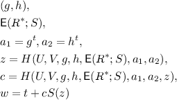
  and sends .

• Verifier calls random oracle twice to get

  

  Then, the verifier homomorphically evaluates , it then computes the value . Finally, accepts if and only if

  $$ \begin{aligned} g^w = a_1(u_1)^c \quad \& \quad h^w = a_2(u_2/g^{my})^c. \end{aligned}$$

Theorem 6.3

Suppose takes $n^{2}$ time to decide for all but finitely many input lengths for any $d=\omega (\log n)$ and the DDH the holds in Schnorr groups, then the above protocol is a $\tilde{O}(n)$-simulatable $(n^2,\delta )$-interactive Proof of Work scheme for any function $\delta (n)>1/n^{o(1)}$.

Proof

Completeness. From before, if $R^* \equiv R_{U,V}$ as is the case for an honest prover, then for any $z\in \mathbb {Z}_q$ we have . Moreover

$$\begin{aligned} g^w = g^{t+cS(z)}=g^t(g^{S(z)})^c=a_1\left( (g^{s_0})(g^{s_1})^z\cdots (g^{s_{nd-1}})^{z^d}\right) ^c, \end{aligned}$$

and

Hardness. Suppose a cheating prover runs in subquadratic time, then by the hardness of Protocol 1.2 with high probability $R^*\not \equiv R_{U,V}$, and so for random z, with overwhelming probability. Suppose this is the case in what follows, namely: . In particular,

Note that can be calculated from the Prover’s first message.

As is standard, we will fix the prover’s first message and (assuming $y\ne y^*$) rewind any two accepting transcripts with distinct challenges to show that $\log _g u_1= \log _h u_2/g^y$. Fix $a_1,a_2$ as above and let $(c,w),(c',w')$ be the two transcripts. Recall that if a transcript is accepted, $g^w=a_1u_1^c$ and $h^w = a_2 (u_2/g^y)^c$. Then,

$$\begin{aligned} g^{w-w'}=u_1^{c-c'} \Rightarrow \log _g u_1 = \frac{w-w'}{c-c'} =\log _h u_2/g^y \Leftarrow h^{w-w'}=(u_2/g^y)^{c-c'} . \end{aligned}$$

Therefore, because $u_1\ne u_2/g^y$ there can be at most one c for which a Prover can convince the verifier. Such a c is chosen with negligible probability.

$\tilde{O}(nd)$ -simulation. Given the verifier’s challenge z, c, (which can simply be sampled uniformly, as above) we can efficiently simulate the transcript with respect to an honest prover as follows:

• Draw public key (g, h).

• Compute the ElGamal Encryption where $R'$ is the polynomial with constant term and zeros elsewhere.

• Draw random w.

• Compute $a_1=\frac{g^w}{g^{cS(z)}}$ and $a_w=\frac{h^w}{h^{cS(z)}}$.

• Output $\left( (g,h),a_1,a_2,z,c,w\right)$.

Notice that do to the semantic security of ElGamal, the transcript output is computationally indistinguishable from that of an honest Prover. Moreover, the simulator runs in $\tilde{O}(nd)$ time, the time to compute $R'$, encrypt, evaluate S and exponentiate. Thus, the protocol is $\tilde{O}(nd)$-simulatable.

Efficiency. The honest prover runs in time $\tilde{O}(n^2)$, because the nd encryptions can be performed in time $\text {polylog}(n)$ each. The verifier takes $\tilde{O}(nd)$ time as well. Note that the homomorphic evaluation requires $O(d\log z^d) = O(d^2\log z) =\text {polylog}(d)$ exponentiations and $d=\text {polylog}(n)$ multiplications.    $\square$

A Stronger Direct Sum Theorem for

In this section, we prove a stronger direct sum theorem (and, thus, non-batchable evaluation) for . That is, we prove Theorem 2.13.

In particular, it is sufficient to define a notion of batchability for parametrized families of functions with a monotonicity constraint. In our case, monotonicity will essentially say “adding more vectors of the same dimension and field size does not make the problem easier.” This is a natural property of most algorithms. Namely, it is the case if for any fixed d, p, is $(n,t,\delta )-batchable$.

Instead, we generalize batchability in a parametrized fashion for .

Definition A.1

A parametrized class, $\mathcal {F}_\rho$, is not $(\ell ,t,\delta )$-batchable on average over $\mathcal {D}_\rho$, a parametrized family of distributions if, for any fixed parameter $\rho$ and algorithm $\mathsf {Batch}_\rho$ that runs in time $\ell (\rho )t(\rho )$ when it is given as input $\ell (\rho )$ independent samples from $D_\rho$, the following is true for all large enough n:

Remark A.2

We use a more generic parameterization of $\mathcal {F}_\rho$ by $\rho$ rather than just n since we need the batch evaluation procedure to have the property that it should still run quickly as n shrinks, as we use downward self-reducibility of , even when p and d remain the same.

We now show how a generalization of the list decoding reduction of [BRSV17a] yields strong batch evaluation bounds. Before we begin, we will present a few Lemmas from the literature to make certain bounds explicit.

First, we present an inclusion-exclusion bound from [CPS99] on the polynomials consistent with a fraction of m input-output pairs, $(x_1,y_1),\ldots ,(x_m,y_m)$. We include a laconic proof here with the given notation for convenience.

Lemma A.3

([CPS99]). Let q be a polynomial over $\mathbb {F}_p$, and define ${{\mathrm{Graph}}}(q):=\{(i,q(i))\ |\ i\in [p]\}$. Let $c>2$, $\delta /2\in (0,1)$, and $m\le p$ such that $m>\frac{c^2(d-1)}{\delta ^2(c-2)}$ for some d. Finally, let $I\subseteq [p]$ such that $|I|=m$. Then, for any set $S=\{(i,y_i)\ |\ i\in I\}$, there are less than $\lceil c/\delta \rceil$ polynomials q of degree at most d that satisfy $|{{\mathrm{Graph}}}(q)\cap S|\ge m\delta /2$.

Corollary A.4

Let S be as in Lemma A.3 with $I=\{m+1,\ldots ,p\}$, for any $m<p$. Then for $m>9d/\delta ^2$, there are at most $3/\delta$ polynomials, q, of degree at most d such that $|{{\mathrm{Graph}}}(q)\cap S|\ge m\delta /2$.

Proof

Reproduced from [CPS99] for convenience; see original for exposition.

Suppose there exist at least $\lceil c/\delta \rceil$ such polynomials. Consider a subset of exactly $N=\lceil c/\delta \rceil$ such polynomials, $\mathcal {F}$. Define $\S _f:=\{(i,f(i))\in {{\mathrm{Graph}}}(f) \cap S\}$, for each $f\in \mathcal {F}$.

$$\begin{aligned} m\ge&\left| \bigcup _{f\in \mathcal {F}} S_f \right| \ge \sum _{f\in \mathcal {F}} |S_f| - \sum _{f,f'\in \mathcal {F}:f\ne f'}|S_f \cap S_{f'}|\\&\ge N\frac{m\delta }{2} - \frac{N(N-1)(d-1)}{2}>\frac{N}{2} \left( m\delta - \frac{c(d-1)}{\delta }\right) \\&\ge \frac{c}{2\delta } \left( m\delta - \frac{c(d-1)}{\delta } \right) = \frac{cm}{2} - \frac{c^2(d-1)}{2\delta ^2}\\&= m + \frac{1}{2}\left( (c-2)m - \frac{c^2(d-1)}{\delta ^2} \right) > m. \end{aligned}$$

   $\square$

Now, we give a theorem based on an efficient list-decoding algorithm, related to Sudan’s, from Roth and Ruckenstein [RR00].

Lemma A.5

([RR00]). List decoding for [n, k] Reed-Solomon (RS) codes over $\mathbb {F}_p$ given a code word with almost $n-\sqrt{2kn}$ errors (for $k>5$), can be performed in

$$\begin{aligned} O\left( n^{3/2}k^{-1/2}\log ^2n + (n-k)^2\sqrt{n/k} + (\sqrt{nk} + \log q)n\log ^2(n/k)\right) \end{aligned}$$

operations over $\mathbb {F}_q$.

Plugging in specific parameters and using efficient list decoding, we get the following corollary which will be useful below.

Corollary A.6

For parameters $n\in \mathbb {N}$ and $\delta \in (0,1)$, list decoding for [m, k] RS over $\mathbb {F}_p$ where $m= \varTheta (d\log n/\delta ^2)$, $k = \varTheta (d)$, $p = O(n^2)$, and $d = \varOmega (\log n)$ can be performed in time

$$\begin{aligned} O\left( \frac{d^2 \log ^{5/2} n {{\mathrm{Arith}}}(n)}{\delta ^5} \right) , \end{aligned}$$

where ${{\mathrm{Arith}}}(n)$ is a time bound on arithmetic operations over prime fields size O(n).

Theorem A.7

For some $k \ge 2$, suppose takes $n^{k-o(1)}$ time to decide for all but finitely many input lengths for any $d = \omega (\log {n})$. Then, for any positive constants $c,\epsilon >0$ and $0<\delta <\varepsilon /2$, is not

-batchable on average over the uniform distribution over its inputs.

Proof

Let $k=2c'+c$ and $p>n^k$. Suppose for the sake of contradiction that is -batchable on average over the uniform distribution.

Let $m=n^{k/(k+c)}$, as before. By Proposition 4.5, with vectors of dimension $d=(\frac{k}{k+c}))^2\log ^2n$ is $(m,m^c)$-downward reducible to with vectors of dimension $\log ^2(n)$, in time $\tilde{O}(m^{c+1})$.

For each $j\in [m^c]$ $X_j=(U^{j1},\ldots ,U^{jk}) \in \{0,1\}^{kmd}$ is the instance of boolean-valued orthogonal vectors from the above reduction. Now, consider splitting these lists in half, $U^{ji}=(U^{ji}_0,U^{ji}_1)$ ($i\in [k]$), such that $(U^{j1}_{a_1},\ldots ,U^{jk}_{a_k})\in \{0,1\}^{kmd/2}$ for $\varvec{a}\in \{0,1\}^k$. Interpret $\varvec{a}$ as binary number in $\{0,\ldots ,2^k-1\}$. Then, define the following $2^k$ sub-problems:

$$\begin{aligned} A^{\varvec{a}}=((U^{j1}_{a_1},\ldots ,U^{jk}_{a_k})),\forall \varvec{a}\in \{0,\ldots ,2^k-1\} \end{aligned}$$

Notice that given solutions to on $\{A^{\varvec{a}}\}_{\varvec{a}\in \{0,1\}^k}$ we can trivially construct a solution to on $X_j$.

Now, draw random $B_j,C_j\in \mathbb {F}_p^{kmd/2}$ and consider the following degree $2^k$ polynomial in x:

$$\begin{aligned} D_j(x) = \sum _{i=1}^{2^k}\delta _i(x)A^{i-1} + (B_j+xC_j)\prod _{i=1}^{2^k}(x-i), \end{aligned}$$

where $\delta _i$ is the unique degree $2^k-1$ polynomial over $\mathbb {F}_p$ that takes value 1 at $i\in [2^k]$ and 0 on all other values in $[2^k]$. Notice that $D_j(i)=A^{i-1}$ for $i\in [2^k]$.

Let $r>2^{k+1}d/\delta ^2\log m$. $D_j(2^k+1),D_j(6),\ldots ,D_j(r+2^k)$. By the properties of $\mathsf {Batch}$ and because the $D_j(\cdot )$’s are independent, $D_1(i),\ldots ,D_{m^c}(i)$ are independent for any fixed i. Thus,

for $\delta r/2$ i’s with probability at least $1-\frac{4}{\delta r}=1-1/\text {polylog}(m)$, by Chebyshev.

Now, because $\delta r/2 > \sqrt{16dr}$, we can run the list decoding algorithm of Roth and Ruckenstein, [RR00], to get a list of all polynomials with degree $\le 2^{k+1}d$ that agree with at least $\delta r /2$ of the values. By Corollary A.4, there are at most $L=3/\delta$ such polynomials.

By a counting argument, there can be at most $2^{k}d\left( {\begin{array}{c}L\\ 2\end{array}}\right) =O(dL^2)$ points in $\mathbb {F}_p$ on which any two of the L polynomials agree. Because $p>n^k>2^kd\left( {\begin{array}{c}L\\ 2\end{array}}\right)$, we can find such a point, $\ell$, by brute-force in $O(L\cdot dL^2\log ^3(dL^2)\log p)$ time, via batch univariate evaluation [Fid72]. Now, to identify the correct polynomials , one only needs to determine the value . To do so, we can recursively apply the above reduction to all the $D_j(\ell )$s until the number of vectors, m, is constant and can be evaluated in time $O(d\log p)$.

Because each recursive iteration cuts m in half, the depth of recursion is $\log (m)$. Additionally, because each iteration has error probability $<4/(\delta r)$, taking a union bound over the $\log (m)$ recursive steps yields an error probability that is $\varepsilon <4\log m/ (\delta r)$.

We can find the prime p via $O(\log m)$ random guesses in $\{m^k+1,\ldots ,2m^k\}$ with overwhelming probability. By Corollary A.6, taking $r=8d\log m/\delta ^2$, Roth and Ruckenstein’s algorithm takes time $O(d^2/\delta ^5\log ^{5/2} m{{\mathrm{Arith}}}(m^k))$ in each recursive call. The brute force procedure takes time $O(d/\delta ^3\log ^3(d/\delta ^2)\log m)$, which is dominated by list decoding time. Reconstruction takes time $O(\log m)$ in each round, and is also dominated. Thus the total run time is

$$\begin{aligned} T =O(m^c(m^{k-\varepsilon }d\log ^2m/\delta ^2 + d^2/\delta ^5\log ^{7/2} m {{\mathrm{Arith}}}(m^k))), \end{aligned}$$

with error probability $\varepsilon <4\log m \delta /d$.    $\square$

References

Ball, M., Dachman-Soled, D., Kulkarni, M., Malkin, T.: Non-malleable codes from average-case hardness: AC0, decision trees, and streaming space-bounded tampering. Cryptology ePrint Archive, Report 2017/1061 (2017). https://eprint.iacr.org/2017/1061
Bitansky, N., Goldwasser, S., Jain, A., Paneth, O., Vaikuntanathan, V., Waters, B.: Time-lock puzzles from randomized encodings. In: Sudan, M. (ed.) Proceedings of the 2016 ACM Conference on Innovations in Theoretical Computer Science, Cambridge, MA, USA, 14–16 January 2016, pp. 345–356. ACM (2016)
Biryukov, A., Khovratovich, D.: Egalitarian computing. In: Holz, T., Savage, S. (eds.) 25th USENIX Security Symposium, USENIX Security 16, Austin, TX, USA, 10–12 August 2016, pp. 315–326. USENIX Association (2016)
Björklund, A., Kaski, P.: How proofs are prepared at Camelot. In: Proceedings of the 2016 ACM Symposium on Principles of Distributed Computing, pp. 391–400. ACM (2016)
Ball, M., Rosen, A., Sabin, M., Vasudevan, P.N.: Average-case fine-grained hardness. In: Hatami, H., McKenzie, P., King, V. (eds.) Proceedings of the 49th Annual ACM SIGACT Symposium on Theory of Computing, STOC 2017, Montreal, QC, Canada, 19–23 June 2017, pp. 483–496. ACM (2017)
Ball, M., Rosen, A., Sabin, M., Vasudevan, P.N.: Proofs of useful work. IACR Cryptology ePrint Archive 2017:203 (2017)
Canetti, R., Chen, Y., Reyzin, L., Rothblum, R.D.: Fiat-Shamir and correlation intractability from strong KDM-secure encryption. In: Nielsen, J.B., Rijmen, V. (eds.) EUROCRYPT 2018. LNCS, vol. 10820, pp. 91–122. Springer, Cham (2018). https://doi.org/10.1007/978-3-319-78381-9_4
Cai, J., Pavan, A., Sivakumar, D.: On the hardness of permanent. In: Meinel, C., Tison, S. (eds.) STACS 1999. LNCS, vol. 1563, pp. 90–99. Springer, Heidelberg (1999). https://doi.org/10.1007/3-540-49116-3_8
Dwork, C., Naor, M.: Pricing via processing or combatting junk mail. In: Brickell, E.F. (ed.) CRYPTO 1992. LNCS, vol. 740, pp. 139–147. Springer, Heidelberg (1993). https://doi.org/10.1007/3-540-48071-4_10
Feigenbaum, J., Fortnow, L.: Random-self-reducibility of complete sets. SIAM J. Comput. 22(5), 994–1005 (1993)
Fiduccia, C.M.: Polynomial evaluation via the division algorithm: the fast Fourier transform revisited. In: Fischer, P.C., Zeiger, H.P., Ullman, J.D., Rosenberg, A.L. (eds.) Proceedings of the 4th Annual ACM Symposium on Theory of Computing, 1–3 May 1972, Denver, Colorado, USA, pp. 88–93. ACM (1972)
Gao, J., Impagliazzo, R.: Orthogonal vectors is hard for first-order properties on sparse graphs. In: Electronic Colloquium on Computational Complexity (ECCC), vol. 23, p. 53 (2016)
Goldreich, O., Rothblum, G.: Simple doubly-efficient interactive proof systems for locally-characterizable sets. Electronic Colloquium on Computational Complexity Report TR17-018, February 2017
Goldreich, O., Rothblum, G.N.: Counting \(t\)-cliques: worst-case to average-case reductions and direct interactive proof systems. In: Electronic Colloquium on Computational Complexity (ECCC), vol. 25, p. 46 (2018)
Horowitz, E.: A fast method for interpolation using preconditioning. Inf. Process. Lett. 1(4), 157–163 (1972)
Jakobsson, M., Juels, A.: Proofs of work and bread pudding protocols (extended abstract). In: Preneel, B. (ed.) Secure Information Networks. ITIFIP, vol. 23, pp. 258–272. Springer, Boston (1999). https://doi.org/10.1007/978-0-387-35568-9_18
Kalai, Y.T., Rothblum, G.N., Rothblum, R.D.: From obfuscation to the security of Fiat-Shamir for proofs. In: Katz, J., Shacham, H. (eds.) CRYPTO 2017, Part II. LNCS, vol. 10402, pp. 224–251. Springer, Cham (2017). https://doi.org/10.1007/978-3-319-63715-0_8
Pass, R.: Simulation in quasi-polynomial time, and its application to protocol composition. In: Biham, E. (ed.) EUROCRYPT 2003. LNCS, vol. 2656, pp. 160–176. Springer, Heidelberg (2003). https://doi.org/10.1007/3-540-39200-9_10
Roth, R.M., Ruckenstein, G.: Efficient decoding of Reed-Solomon codes beyond half the minimum distance. IEEE Trans. Inf. Theory 46(1), 246–257 (2000)
Sherstov, A.A.: Strong direct product theorems for quantum communication and query complexity. SIAM J. Comput. 41(5), 1122–1165 (2012)
Stebila, D., Kuppusamy, L., Rangasamy, J., Boyd, C., Gonzalez Nieto, J.: Stronger difficulty notions for client puzzles and denial-of-service-resistant protocols. In: Kiayias, A. (ed.) CT-RSA 2011. LNCS, vol. 6558, pp. 284–301. Springer, Heidelberg (2011). https://doi.org/10.1007/978-3-642-19074-2_19
Williams, R.: A new algorithm for optimal 2-constraint satisfaction and its implications. Theor. Comput. Sci. 348(2–3), 357–365 (2005)
Williams, V.V.: Hardness of easy problems: basing hardness on popular conjectures such as the strong exponential time hypothesis. In: Proceedings of International Symposium on Parameterized and Exact Computation, pp. 16–28 (2015)
Williams, R.R.: Strong ETH breaks with Merlin and Arthur: short non-interactive proofs of batch evaluation. In: 31st Conference on Computational Complexity, CCC 2016, 29 May to 1 June 2016, Tokyo, Japan, pp. 2:1–2:17 (2016)
Acknowledgements
We are grateful to Oded Goldreich and Guy Rothblum for clarifying definitions of direct sum theorems, and for the suggestion of using interaction to increase the gap between solution and verification in our PoWs. We would also like to thank Tal Moran and Vinod Vaikuntanathan for several useful discussions. We also thank the anonymous reviewers for comments and references.
The bulk of this work was performed while the authors were at IDC Herzliya’s FACT center and supported by NSF-BSF Cyber Security and Privacy grant #2014/632, ISF grant #1255/12, and by the ERC under the EU’s Seventh Framework Programme (FP/2007-2013) ERC Grant Agreement #07952. Marshall Ball is supported in part by the Defense Advanced Research Project Agency (DARPA) and Army Research Office (ARO) under Contract #W911NF-15-C-0236, NSF grants #CNS-1445424 and #CCF-1423306, the Leona M. & Harry B. Helmsley Charitable Trust, ISF grant no. 1790/13, and the Check Point Institute for Information Security. Alon Rosen is also supported by ISF grant no. 1399/17. Manuel Sabin is also supported by the National Science Foundation Graduate Research Fellowship under Grant #DGE-1106400. Prashant Nalini Vasudevan is also supported by the IBM Thomas J. Watson Research Center (Agreement #4915012803), by NSF Grants CNS-1350619 and CNS-1414119, and by the Defense Advanced Research Projects Agency (DARPA) and the U.S. Army Research Office under contracts W911NF-15-C-0226 and W911NF-15-C-0236.
Author information
Authors and Affiliations
Corresponding author
Editor information
Editors and Affiliations