Co-Regularised Support Vector Regression

Abstract

We consider a semi-supervised learning scenario for regression, where only few labelled examples, many unlabelled instances and different data representations (multiple views) are available. For this setting, we extend support vector regression with a co-regularisation term and obtain co-regularised support vector regression (CoSVR). In addition to labelled data, co-regularisation includes information from unlabelled examples by ensuring that models trained on different views make similar predictions. Ligand affinity prediction is an important real-world problem that fits into this scenario. The characterisation of the strength of protein-ligand bonds is a crucial step in the process of drug discovery and design. We introduce variants of the base CoSVR algorithm and discuss their theoretical and computational properties. For the CoSVR function class we provide a theoretical bound on the Rademacher complexity. Finally, we demonstrate the usefulness of CoSVR for the affinity prediction task and evaluate its performance empirically on different protein-ligand datasets. We show that CoSVR outperforms co-regularised least squares regression as well as existing state-of-the-art approaches for affinity prediction. Code and data related to this chapter are available at: https://doi.org/10.6084/m9.figshare.5427241.

1 Introduction

We investigate an algorithm from the intersection field of semi-supervised and multi-view learning. In semi-supervised learning the lack of a satisfactory number of labelled examples is compensated by the usage of many unlabelled instances from the respective feature space. Multi-view regression algorithms utilise different data representations to train models for a real-valued quantity. Ligand affinity prediction is an important learning task from chemoinformatics since many drugs act as protein ligands. It can be assigned to this learning scenario in a very natural way. The aim of affinity prediction is the determination of binding affinities for small molecular compounds—the ligands—with respect to a bigger protein using computational methods. Besides a few labelled protein-ligand pairs, millions of small compounds are gathered in molecular databases as ligand candidates. Many different data representations—the so-called molecular fingerprints or views—exist that can be used for learning. Affinity prediction and other applications suffer from little label information and the need to choose the most appropriate view for learning. To overcome these difficulties, we propose to apply an approach called co-regularised support vector regression. We are the first to investigate support vector regression with co-regularisation, i.e., a term penalising the deviation of predictions on unlabelled instances. We investigate two loss functions for the co-regularisation. In addition to variants of our multi-view algorithm with a reduced number of optimisation variables, we also derive a transformation into a single-view method. Furthermore, we prove upper bounds for the Rademacher complexity, which is important to restrict the capacity of the considered function class to fit random data. We will show that our proposed algorithm outperforms affinity prediction baselines.

The strength of a protein-compound binding interaction is characterised by the real-valued binding affinity. If it exceeds a certain limit, the small compound is called a ligand of the protein. Ligand-based classification models can be trained to distinguish between ligands and non-ligands of the considered protein (e.g., with support vector machines [6]). Since framing the biological reality in a classification setting represents a severe simplification of the biological reality, we want to predict the strength of binding using regression techniques from machine learning. Both classification and regression methods are also known under the name of ligand-based virtual screening. (In the context of regression, we will use the name ligands for all considered compounds.) Various approaches like neural networks [7] have been applied. However, support vector regression (SVR) is the state-of-the-art method for affinity prediction studies (e.g., [12]).

As mentioned above, in the context of affinity prediction one is typically faced with the following practical scenario: for a given protein, only few ligands with experimentally identified affinity values are available. In contrast, the number of synthesizable compounds gathered in molecular databases (such as ZINC, BindingDB, ChEMBL¹) is huge which can be used as unlabelled instances for learning. Furthermore, different free or commercial vectorial representations or molecular fingerprints for compounds exist. Originally, each fingerprint was designed towards a certain learning purpose and, therefore, comprises a characteristic collection of physico-chemical or structural molecular features [1], for example, predefined key properties (Maccs fingerprint) or listed subgraph patterns (ECFP fingerprints).

The canonical way to deal with multiple fingerprints for virtual screening would be to extensively test and compare different fingerprints [6] or perform time-consuming preprocessing feature selection and recombination steps [8]. Other attempts to utilise multiple views for one prediction task can be found in the literature. For example, Ullrich et al. [13] apply multiple kernel learning. However, none of these approaches include unlabelled compounds in the affinity prediction task. The semi-supervised co-regularised least squares regression (CoRLSR) algorithm of Brefeld et al. [4] has been shown to outperform single-view regularised least squares regression (RLSR) for UCI datasets². Usually, SVR shows very good predictive results having a lower generalisation error compared to RLSR. Aside from that, SVR represents the state-of-the-art in affinity prediction (see above). For this reason, we define co-regularised support vector regression (CoSVR) as an $\varepsilon$-insensitive version of co-regularisation. In general, CoSVR—just like CoRLSR—can be applied on every regression task with multiple views on data as well as labelled and unlabelled examples. However, learning scenarios with high-dimensional sparse data representations and very few labelled examples—like the one for affinity prediction—could benefit from approaches using co-regularisation. In this case, unlabelled examples can contain information that could not be extracted from a few labelled examples because of the high dimension and sparsity of the data representation.

A view on data is a representation of its objects, e.g., with a particular choice of features in . We will see that feature mappings are closely related to the concept of kernel functions, for which reason we introduce CoSVR theoretically in the general framework of kernel methods. Within the research field of multi-view learning, CoSVR and CoRLSR can be assigned to the group of co-training style [16] approaches that simultaneously learn multiple predictors, each related to a view. Co-training style approaches enforce similar outcomes of multiple predictor functions for unlabelled examples, measured with respect to some loss function. In the case of co-regularisation for regression the empirical risks of multiple predictors (labelled error) plus an error term for unlabelled examples (unlabelled error, co-regularisation) are minimised.

The idea for mutual influence of multiple predictors appeared in the paper of Blum and Mitchell [2] on classification with co-training. Wang et al. [14] combined the technique of co-training with SVR with a technique different from co-regularisation. Analogous to CoSVR, CoRLSR is a semi-supervised and multi-view version of RLSR that requires the solution of a large system of equations [4]. A co-regularised version for support vector machine classification SVM-2K already appeared in the paper of Farquhar et al. [5], where the authors define a co-regularisation term via the $\varepsilon$-insensitive loss on labelled examples. It was shown by Sindhwani and Rosenberg [11] that co-regularised approaches applying the squared loss function for the unlabelled error can be transformed into a standard SVR optimisation with a particular fusion kernel. A bound on the empirical Rademacher complexity for co-regularised algorithms with Lipschitz continuous loss function for the labelled error and squared loss function for the unlabelled error was proven by Rosenberg and Bartlett [9].

A preliminary version of this paper was published at the Data Mining in Biomedical Informatics and Healthcare workshop held at ICDM 2016. There, we considered only the CoSVR special case $\varepsilon$-CoSVR and its variants with reduced numbers of variables (for the definitions consult Definitions 1 –3 below) focusing the application of ligand affinity prediction. The $\ell _2$-CoSVR case (see below) with its theoretical properties (Lemmas 1(ii) - 3(ii), 6(ii)) and practical evaluation, as well as the faster $\varSigma$-CoSVR (Sect. 3.3) variant are novel contributions in the present paper.

In the following section, we will present a short summary of kernels and multiple views, as well as important notation. We define CoSVR and variants of the base algorithm in Sect. 3. In particular, a Rademacher bound for CoSVR will be proven in Sect. 3.5. Subsequently, we provide a practical evaluation of CoSVR for ligand affinity prediction in Sect. 4 and conclude with a brief discussion in Sect. 5.

2 Kernels and Multiple Views

We consider an arbitrary instance space $\mathcal {X}$ and the real numbers as label space $\mathcal {Y}$. We want to learn a function f that predicts a real-valued characteristic of the elements of $\mathcal {X}$. Suppose for training purposes we have sets $X = \{x_1, \ldots , x_n\} \subset \mathcal {X}$ of labelled and $Z = \{z_1, \ldots , z_m\} \subset \mathcal {X}$ of unlabelled instances at our disposal, where typically $m \gg n$ holds true. With $\{y_1, \ldots , y_n\} \subset \mathcal {Y}$ we denote the respective labels of X. Furthermore, assume the data instances can be represented in M different ways. More formally, for $v \in \{1,\ldots ,M\}$ there are functions $\varPhi _v:\mathcal {X} \rightarrow \mathcal {H}_v$, where $\mathcal {H}_v$ is an appropriate inner product space. Given an instance $x \in \mathcal {X}$, we say that $\varPhi _v(x)$ is the v-th view of x. If $\mathcal {H}_v$ equals for some finite dimension d, the intuitive names (v-th) feature mapping and feature space are used for $\varPhi _v$ and $\mathcal {H}_v$, respectively. If in the more general case $\mathcal {H}_v$ is a Hilbert space, d can even be infinite (see below). For view v the predictor function is denoted with (single) view predictor. View predictors can be learned independently for each view utilising an appropriate regression algorithm like SVR or RLSR. As a special case we consider concatenated predictors $f_v$ in Sect. 4 where the corresponding view v results from a concatenation of finite dimensional feature representations $\varPhi _1, \ldots , \varPhi _M$. Having different views on the data, an alternative is to learn M predictors simultaneously that depend on each other, satisfying an optimisation criterion involving all views at once. Such a criterion could be the minimisation of the labelled error in line with co-regularisation which will be specified in the following subsection. The final predictor f will then be the average of the predictors $f_v$.

A function is said to be a kernel if it is symmetric and positive semi-definite. Indeed, for every kernel k there is a feature mapping $\varPhi :\mathcal {X} \rightarrow \mathcal {H}$ such that $\mathcal {H}$ is a reproducing kernel Hilbert space (RKHS) and $k(x_1,x_2) = \langle \varPhi (x_1), \varPhi (x_2) \rangle _{\mathcal {H}}$ holds true for all $x_1,x_2 \in \mathcal {X}$ (Mercer’s theorem). Thus, the function k is the corresponding reproducing kernel of $\mathcal {H}$, and for $x \in \mathcal {X}$ the mappings $\langle \varPhi (x), \varPhi (\cdot )\rangle = k(x,\cdot )$ are functions defined on $\mathcal {X}$. Choosing RKHSs $\mathcal {H}_v$ of multiple kernels $k_v$ as candidate spaces for the predictors $f_v$, the representer theorem of Schölkopf et al. [10] allows for a parameterisation of the optimisation problems for co-regularisation presented below. A straightforward modification of the representer theorem’s proof leads to a representation of the predictors $f_v$ as finite kernel expansion

$$\begin{aligned} f_v(\cdot )=\sum \limits _{i=1}^{n} \pi _{vi} k_v(x_i, \cdot ) + \sum \limits _{j=1}^m \pi _{v(j+n)}k_v(z_j,\cdot ) \end{aligned}$$

(1)

with linear coefficients , centered at labelled and unlabelled instances $x_i \in X$ and $z_j \in Z$, respectively.

The kernel matrices $K_v = \left\{ k_v(x_i,x_j)\right\} _{i,j=1}^{n+m}$ are the Gram matrices of the v-th view kernel $k_v$ over labelled and unlabelled examples and have decompositions into an upper and a lower part and , respectively. We will consider the submatrices $k(Z,x) := (k(z_1,x), \ldots , k(z_m,x))^T\text { and }k(Z, Z) := \{k(z_j, z_{j'})\}_{j, j' = 1}^{m}$ of a Gram matrix with kernel k. If $\mathcal {H}_1$ and $\mathcal {H}_2$ are RKHSs then their sum space $\mathcal {H}_{\varSigma }$ is defined as $\mathcal {H}_{\varSigma } := \{f : f = f_1 + f_2, f_1 \in \mathcal {H}_1, f_2 \in \mathcal {H}_2\}$. With we denote the vector of labels. We will abbreviate $v\in \{1,\ldots ,M\}$ with $v \in [\![M]\!]$. And finally, we will utilise the squared loss $\ell _2(y,y') = \Vert y-y'\Vert ^2$ and the $\varepsilon$-insensitive loss $\ell _{\varepsilon }(y,y') = \max \{0,|y-y'|-\varepsilon \}$, $y, y' \in \mathcal {Y}$.

3 The CoSVR Algorithm: Variants and Properties

3.1 Base CoSVR

In order to solve a regression task in the presence of multiple views $v=1,\ldots ,M$, the approach of co-regularisation is to jointly minimise two error terms involving M predictor functions $f_1, \ldots , f_M$. Firstly, every view predictor $f_v$ is intended to have a small training error with respect to labelled examples. Secondly, the difference between pairwise view predictions over unlabelled examples should preferably be small. We introduce co-regularised support vector regression (CoSVR) as an $\varepsilon$-insensitive loss realisation of the co-regularisation principle.

Definition 1

For $v \in \{1,\ldots ,M\}$ let $\mathcal {H}_v$ be RKHSs. The co-regularised empirical risk minimisation

$$\begin{aligned} \underset{f_v \in \mathcal {H}_v}{\min }~&\sum \limits _{v=1}^M \left( \frac{\nu _v}{2} \Vert f_v\Vert ^2+ \sum \limits _{i=1}^n \ell ^L(y_i,f_v(x_i)) \right) \\&+\lambda \sum \limits _{u,v=1}^M \sum \limits _{j=1}^m \ell ^U(f_u(z_j), f_v(z_j)),\nonumber \end{aligned}$$

(2)

where $\nu _v,\lambda \ge 0$ is called co-regularised support vector regression (CoSVR) if $\ell ^L = \ell _{\varepsilon ^L}$, $\varepsilon ^L \ge 0$, and $\ell ^U$ is an arbitrary loss function for regression. Furthermore, we define $\varepsilon$-CoSVR to be the special case where $\ell ^U = \ell _{\varepsilon ^U}$, $\varepsilon ^U \ge 0$, as well as $\ell _2$-CoSVR to satisfy $\ell ^U = \ell _2$.

The minimum in (2) is taken over all $f_v$, $v = 1,\ldots , M$. For reasons of simplification we will abbreviate $\min _{f_1 \in \mathcal {H}_1, \ldots , f_M \in \mathcal {H}_M}$ with $\min _{f_v \in \mathcal {H}_v}$. Note that the loss function parameters $\varepsilon ^L$ and $\varepsilon ^U$ can have different values. The parameters $\nu _v$ and $\lambda$ are trade-off parameters between empirical risk and co-regularisation term. The added norm terms $\Vert f_v\Vert$ prevent overfitting. We will also refer to the empirical risk term with loss function $\ell ^L$ as labelled error and to the co-regularisation term with $\ell ^U$ as unlabelled error. In the case of $\ell ^L = \ell ^U = \ell _2$, the optimisation in (2) is known as co-regularised least squares regression (CoRLSR). Brefeld et al. [4] found a closed form solution for CoRLSR as linear system of equations in $M(n+m)$ variables. In the following, we present a solution for $\varepsilon$-CoSVR and $\ell _2$-CoSVR.

Lemma 1

Let $\nu _v, \lambda , \varepsilon ^L, \varepsilon ^U \ge 0$. We use the notation introduced above. In particular, denote the kernel expansion coefficients of the single view predictors $f_v$ from (1), whereas and are dual variables.

• (i) The dual optimisation problem of $\varepsilon$-CoSVR equals

  

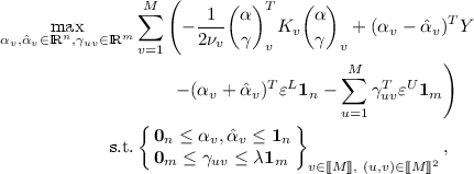
  where $\pi _v^T = \tfrac{1}{\nu _v} (\alpha ~|~ \gamma )^T_v$ and $(\alpha ~|~ \gamma )^T_v = (\alpha _v - \hat{\alpha }_v ~|~ \sum _{u=1}^M (\gamma _{uv}-\gamma _{vu}))^T$.

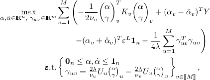
• (ii) The dual optimisation problem of $\ell _2$-CoSVR is

  

  where $\pi _v^T = \tfrac{1}{\nu _v}(\alpha ~|~ \gamma )_v^T$ and $(\alpha ~|~ \gamma )_v^T = (\alpha _v - \hat{\alpha }_v ~|~ \sum _{u=1}^M (\gamma _{uv}-\gamma _{vu}))^T$.

Remark 1

The proofs of Lemma 1 as well as Lemmas 2 and 3 below use standard techniques from Lagrangian dualisation (e.g., [3]). They can be found in our CoSVR repository (see footnote 3).

We choose the concatenated vector representation in order to show the correspondence between the two problems $\varepsilon$-CoSVR and $\ell _2$-CoSVR and further CoSVR variants below. Additionally, the similarities with and differences to the original SVR dual problem are obvious. We will refer to the optimisation in Lemma 1 as the base CoSVR algorithms.

3.2 Reduction of Variable Numbers

The dual problems in Lemma 1 are quadratic programs. Both depend on $2Mn + M^2m$ variables, where $m \gg n$. If the number of views M and the number of unlabelled examples m are large, the base CoSVR algorithm might cause problems with respect to runtime because of the large number of resulting variables. In order to reduce this number, we define modified versions of base CoSVR. We denote the variant with a modification in the labelled error with CoSVR$^{mod}$ and in the unlabelled error with CoSVR$_{mod}$.

Modification of the Empirical Risk. In base CoSVR the empirical risk is meant to be small for each single view predictor individually using examples and their corresponding labels. In the CoSVR$^{mod}$ variant the average prediction, i.e., the final predictor, is applied to define the labelled error term.

Definition 2

The co-regularised support vector regression problem with modified constraints for the labelled examples (CoSVR$^{mod}$) is defined as

$$\begin{aligned} \underset{f_v \in \mathcal {H}_v}{\min }&\sum \limits _{v=1}^M \frac{\nu _v}{2} \Vert f_v\Vert ^2 + \sum \limits _{i=1}^n \ell _{\varepsilon ^L}(y_i,f^{\mathrm {avg}}(x_i)) \\&+ \lambda \sum \limits _{u,v=1}^M \sum \limits _{j=1}^m \ell ^U \left( f_u(z_j),f_v(z_j) \right) , \end{aligned}$$

where $f^{\mathrm {avg}} := \tfrac{1}{M}\sum _{v=1}^M f_v$ is the average of all single view predictors. We denote the case $\ell ^U = \ell _{\varepsilon ^U}$, $\varepsilon ^U \ge 0$, with $\varepsilon$-CoSVR$^{mod}$ and the case $\ell ^U = \ell _2$ with $\ell _2$-CoSVR$^{mod}$.

In the following lemma we present solutions for $\varepsilon$-CoSVR$^{mod}$ and $\ell _2$-CoSVR$^{mod}$.

Lemma 2

Let $\nu _v, \lambda , \varepsilon ^L, \varepsilon ^U \ge 0$. We utilise dual variables and .

• (i) The $\varepsilon$-CoSVR$^{mod}$ dual optimisation problem can be written as

  

  where $\pi _v^T = \tfrac{1}{\nu _v} (\alpha ~|~ \gamma )_v^T$ and $(\alpha ~|~ \gamma )_v^T = (\tfrac{1}{M}(\alpha - \hat{\alpha }) ~|~\sum _{u=1}^M(\gamma _{uv}-\gamma _{vu}) )^T$.

• (ii) The $\ell _2$-CoSVR$^{mod}$ dual optimisation problem equals

  

  where $\pi _v^T = \tfrac{1}{\nu _v} (\alpha ~|~ \gamma )_v^T$ and $(\alpha ~|~ \gamma )_v^T = (\tfrac{1}{M}(\alpha - \hat{\alpha }) ~|~ \sum _{u=1}^M(\gamma _{uv}-\gamma _{vu}))^T$.

We can also reduce the number of variables more effectively using modified constraints for the co-regularisation term. Whereas the CoSVR$^{mod}$ algorithm is rather important from a theoretical perspective (see Sect. 3.3), the variant presented in the next section is very beneficial from a practical perspective if the number of views M is large.

Modification of the Co-regularisation. The unlabelled error term of base CoSVR bounds the pairwise distances of view predictions, whereas now in CoSVR$_{mod}$ only the disagreement between predictions of each view and the average prediction of the residual views will be taken into account.

Definition 3

We consider RKHSs $\mathcal {H}_1,\ldots , \mathcal {H}_M$ as well as constants $\varepsilon ^L, \varepsilon ^U, \nu _v, \lambda \ge 0$. The co-regularised support vector regression problem with modified constraints for the unlabelled examples (CoSVR$_{mod}$) is defined as

$$\begin{aligned} \underset{f_v \in \mathcal {H}_v}{\min }&\sum \limits _{v=1}^M \left( \frac{\nu _v}{2} \Vert f_v\Vert ^2 + \sum \limits _{i=1}^n \ell _{\varepsilon ^L}(y_i,f_v(x_i)) \right) \\&+ \lambda \sum \limits _{v=1}^M \sum \limits _{j=1}^m \ell ^U \left( f_v^{\mathrm {avg}}(z_j),~f_v(z_j) \right) , \nonumber \end{aligned}$$

(3)

where now $f_{v}^{\mathrm {avg}} := \tfrac{1}{M-1}\sum _{u =1}^{M, u \ne v} f_u$ is the average of view predictors besides view v. We denote the case $\ell ^U = \ell _{\varepsilon ^U}$, $\varepsilon ^U \ge 0$, with $\varepsilon$-CoSVR$_{mod}$ and the case $\ell ^U = \ell _2$ with $\ell _2$-CoSVR$_{mod}$.

Again we present solutions for $\varepsilon$-CoSVR$_{mod}$ and $\ell _2$-CoSVR$_{mod}$.

Lemma 3

Let $\nu _v, \lambda , \varepsilon ^L, \varepsilon ^U \ge 0$. We utilise dual variables and , as well as $\gamma _v^{avg} := \frac{1}{M-1}\sum _{u=1}^{M, u \ne v} \gamma _u$ and $\hat{\gamma }_v^{avg} := \frac{1}{M-1}\sum _{u=1}^{M, u\ne v} \hat{\gamma }_u$ analogous to the residual view predictor average.

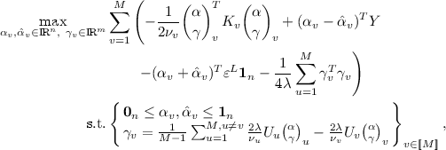
• (i) The $\varepsilon$-CoSVR$_{mod}$ dual optimisation problem can be written as

  

  where $\pi _v^T = \tfrac{1}{\nu _v}(\alpha ~|~ \gamma )^T_v$ and $(\alpha ~|~ \gamma )^T_v = (\alpha _v - \hat{\alpha }_v ~|~ (\gamma _v -\gamma _v^{avg}) - (\hat{\gamma }_v - \hat{\gamma }_v^{avg}))^T$.

• (ii) The $\ell _2$-CoSVR$_{mod}$ dual optimisation problem equals

  

  where $\pi _v^T = \tfrac{1}{\nu _v}(\alpha ~|~ \gamma )_v^T$ and $(\alpha ~|~ \gamma )_v^T = (\alpha _v - \hat{\alpha }_v ~|~ \gamma _v -\gamma _v^{avg})^T$.

Remark 2

If we combine the modifications in the labelled and unlabelled error term we canonically obtain the variants $\varepsilon$-CoSVR$^{mod}_{mod}$ and $\ell _2$-CoSVR$^{mod}_{mod}$.

In the base CoSVR versions the semi-supervision is realised with proximity constraints on pairs of view predictions. We show in the following lemma that the constraints of the closeness of one view prediction to the average of the residual predictions implies a closeness of every pair of predictions.

Lemma 4

Up to constants, the unlabelled error bound of CoSVR$_{mod}$ is also an upper bound of the unlabelled error of base CoSVR.

Proof

We consider the settings of Lemmas 1(i) and 3(i). For part (ii) the proof is equivalent with $\varepsilon ^U = 0$. In the case of $M=2$, modified and base algorithm fall together which shows the claim. Now let $M > 2$. Because of the definition of the $\varepsilon$-insensitive loss we know that $|f_v(z_j) - f_v^{\mathrm {avg}}(z_j)| \le \varepsilon ^U + c_{vj},$ where $c_{vj} \ge 0$ is the actual loss value for fixed v and j. We denote $c_j := \max _{v \in \{1,\ldots ,M\}} \{c_{1j},\dots ,c_{Mj}\}$ and, hence, $|f_v(z_j) - f_v^{\mathrm {avg}}(z_j)| \le \varepsilon ^U + c_j$ for all $v \in \{1, \ldots , M\}$. Now we conclude for $j \in \{1,\ldots ,m\}$ and $(u,v) \in \{1, \ldots , M\}^2$

$$\begin{aligned}&|f_u(z_j) - f_v(z_j)|\\&\le |f_u(z_j) - f_u^{\mathrm {avg}}(z_j)| + |f_u^{\mathrm {avg}}(z_j) - f_v^{\mathrm {avg}}(z_j)| + |f_v^{\mathrm {avg}}(z_j) - f_v(z_j)| \\&\le \varepsilon ^U + c_j + \tfrac{1}{M-1}|f_v(z_j) -f_u(z_j)| + \varepsilon ^U + c_j, \end{aligned}$$

and therefore, $|f_u(z_j) - f_v(z_j)| \le \tfrac{2(M-1)}{M-2} (\varepsilon ^U + c_j).$ As a consequence we deduce from $\sum _{v=1}^M \sum _{j=1}^m \ell _{\varepsilon ^U} (f_v^{\mathrm {avg}}(z_j), f_v(z_j)) \le M\sum _{j=1}^m c_j =: B$ that also the labelled error of CoSVR can be bounded $\sum _{u,v=1}^M \sum _{j=1}^m \ell _{\tilde{\varepsilon }} (f_u(z_j), f_v(z_j))\le \tilde{B}$ for $\tilde{\varepsilon } = \tfrac{2(M-1)}{M-2} \varepsilon ^U$ and $\tilde{B} = \tfrac{2M(M-1)}{(M-2)} B$, which finishes the proof.    $\square$

3.3 $\varSigma$-CoSVR

Sindhwani and Rosenberg [11] showed that under certain conditions co-regularisation approaches of two views exhibit a very useful property. If $\ell ^U = \ell _2$ and the labelled loss is calculated utilising an arbitrary loss function for the average predictor $f^{avg}$, the resulting multi-view approach is equivalent with a single-view approach of a fused kernel. We use the notion from Sect. 2.

Definition 4

Let $\lambda , \nu _1,\nu _2,\varepsilon ^L \ge 0$ be parameters and the Gram submatrices k(Z, x) and k(Z, Z) be defined as in Sect. 2. We consider a merged kernel $k_{\varSigma }$ from two view kernels $k_1$ and $k_2$

$$\begin{aligned} k_{\varSigma }(x,x'):=k^{\oplus }(x,x') - k^{\ominus }(Z,x)^T \left( \tfrac{1}{\lambda }I_m + k^{\oplus }(Z,Z)\right) ^{-1} k^{\ominus }(Z,x'), \end{aligned}$$

(4)

for $x,x' \in \mathcal {X}$, where $k^{\oplus } := \tfrac{1}{\nu _1}k_1 + \frac{1}{\nu _2}k_2$ and $k^{\ominus } := \tfrac{1}{\nu _1}k_1 - \frac{1}{\nu _2}k_2$. We denote the SVR optimisation

$$\begin{aligned} \underset{f \in \mathcal {H}_{\varSigma }}{{\text {argmin}}} \Vert f\Vert ^2 + \sum \limits _{i=1}^n \ell _{\varepsilon ^L}(y_i,\tfrac{1}{2}f(x_i)), \end{aligned}$$

(5)

$\varSigma$-co-regularised support vector regression ($\varSigma$-CoSVR), where $\mathcal {H}_{\varSigma }$ is the RKHS of $k_{\varSigma }$.

Please notice that for each pair $(x, x')$ the value of $k_{\varSigma }(x, x')$ is calculated in (4) with $k_1$ and $k_2$ including not only x and $x'$ but also unlabelled examples $z_1, \ldots , z_m$. Hence, the optimisation problem in (5) is a standard SVR with additional information about unlabelled examples incorporated in the RKHS $\mathcal {H}_{\varSigma }$.

Lemma 5

The algorithms $\ell _2$-CoSVR$^{mod}$ and $\varSigma$-CoSVR are equivalent and $\mathcal {H}_{\varSigma }$ is the sum space .

Proof

The proof is an application of Theorem 2.2. of Sindhwani and Rosenberg [11] for the loss function V being equal to the $\varepsilon$-insensitive loss with $\varepsilon = \varepsilon ^L$, the parameter of the labelled error of $\ell _2$-CoSVR$^{mod}$.    $\square$

As $\varSigma$-CoSVR can be solved as a standard SVR algorithm we obtained a much faster co-regularisation approach. The information of the two views and the unlabelled examples are included in the candidate space $\mathcal {H}_{\varSigma }$ and associated kernel $k_{\varSigma }$.

3.4 Complexity

The CoSVR variants and CoRLSR mainly differ in the number of applied loss functions and the strictness of constraints. This results in different numbers of variables and constraints in total, as well as potentially non-zero variables (referred to as sparsity, compare Table 1). All presented problems are convex QPs with positive semi-definite matrices in the quadratic terms. As the number m of unlabelled instances in real-world problems is much greater than n, the runtime of a QP-solver is dominated by the respective second summand in the constraints column of Table 1. Because of the $\varepsilon$-insensitive loss the number of actual non-zero variables in the learned model will be even smaller for the CoSVR variants than the numbers reported in the sparsity column of Table 1. In particular, for the modified variants this will allow for a more efficient model storage compared to CoRLSR. Indeed, according to the Karush-Kuhn-Tucker conditions (e.g., [3]), only for active inequality constraints the corresponding dual $\gamma$-variables can be non-zero. In this sense the respective unlabelled $z_j \in Z$ are unlabelled support vectors. This consideration is also valid for the $\alpha$-variables and support vectors $x_i \in X$ as we use the $\varepsilon$-insensitive loss for the labelled error in all CoSVR versions. And finally, in the two-view case with $M=2$ the modified version with respect to the unlabelled error term and the base version coincide.

Table 1. Number of variables, constraints, and potential non-zero variables for different CoSVR versions and CoRLSR. The respective CoSVR$^{mod}$ variant is included by cancelling the $\{M\}$-factor.

3.5 A Rademacher Bound for CoSVR

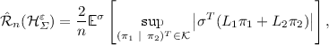
Similarly to the result of Rosenberg and Bartlett [9] we want to prove a bound on the empirical Rademacher complexity $\hat{\mathcal {R}}_n$ of CoSVR in the case of $M=2$. Note that, despite the proof holding for the special case of $M=2$, the CoSVR method in general is applicable to arbitrary numbers of views. The empirical Rademacher complexity is a data-dependent measure for the capacity of a function class $\mathcal {H}$ to fit random data and is defined as

$$\begin{aligned} \hat{\mathcal {R}}_n(\mathcal {H}) = \mathbb {E}^{\sigma }\left[ \underset{f \in \mathcal {H}}{\sup } \left| \frac{2}{n} \sum \limits _{i=1}^n \sigma _i f(x_i) \right| : \{x_1, \ldots , x_n\} = X\right] . \end{aligned}$$

The random data are represented via Rademacher random variables $\sigma = (\sigma _1, \ldots , \sigma _n)^T$. We consider $\varepsilon$-CoSVR and $\ell _2$-CoSVR and define bounded versions $\mathcal {H}_{\varSigma }^{\varepsilon }$ and $\mathcal {H}_{\varSigma }^{2}$ of the sum space $\mathcal {H}_{\varSigma }$ from Sect. 2 for the corresponding versions. Obviously, a pair of kernel expansion coefficients (see (1)) represents an element of $\mathcal {H}_{\varSigma }$. For $\varepsilon$-CoSVR and $\ell _2$-CoSVR we set

$$\begin{aligned} \mathcal {H}_{\varSigma }^{\varepsilon }&:= \left\{ (\pi _1,\pi _2) \in \mathcal {H}_{\varSigma }: -\mu 1_{n+m} \le \pi _1, \pi _2 \le \mu 1_{n+m} \right\} , \quad \text { and } \end{aligned}$$

(6)

$$\begin{aligned} \mathcal {H}_{\varSigma }^{2}&:= \left\{ (\pi _1,\pi _2) \in \mathcal {H}_{\varSigma }\right. : \nu _1 \pi _1^T K_1 \pi _1 + \nu _2 \pi _2^T K_2 \pi _2 \nonumber \\&~~~\left. + \lambda (U_1\pi _1 - U_2\pi _2)^T(U_1\pi _1 - U_2\pi _2) \le 1\right\} , \end{aligned}$$

(7)

respectively. In (6) $\mu$ is an appropriate constant according to Lemmas 1 and 2. The definition in (7) follows the reasoning of Rosenberg and Bartlett [9]. Now we derive a bound on the empirical Rademacher complexity of $\mathcal {H}_{\varSigma }^{\varepsilon }$ and $\mathcal {H}_{\varSigma }^{2}$, respectively. We point out that the subsequent proof is also valid for the modified versions with respect to the empirical risk. For two views the base and modified versions with respect to the co-regularisation fall together anyway. For reasons of simplicity, in the following lemma and proof we omit $^{mod}$ and $_{mod}$ for the CoSVR variants. Furthermore, we will apply the infinity vector norm $\Vert v\Vert _{\infty }$ and row sum matrix norm $\Vert L\Vert _{\infty }$ (consult, e.g., Werner [15]).

Lemma 6

Let $\mathcal {H}_{\varSigma }^{\varepsilon }$ and $\mathcal {H}_{\varSigma }^{2}$ be the function spaces in (6) and (7) and, without loss of generality, let $\mathcal {Y} = [-1,1]$.

• (i) The empirical Rademacher complexity of $\varepsilon$-CoSVR can be bounded via

  $$\begin{aligned} \hat{\mathcal {R}}_n (\mathcal {H}_{\varSigma }^{\varepsilon }) \le \frac{2s}{n}\mu (\Vert L_1\Vert _{\infty } + \Vert L_2\Vert _{\infty }), \end{aligned}$$

  where $\mu$ is a constant dependent on the regularisation parameters and s is the number of potentially non-zero variables in the kernel expansion vector $\pi \in \mathcal {H}_{\varSigma }^{\varepsilon }$.

• (ii) The empirical Rademacher complexity of $\ell _2$-CoSVR has a bound

  $$\begin{aligned} \hat{\mathcal {R}}_n (\mathcal {H}_{\varSigma }^{2}) \le \frac{2}{n} \sqrt{tr_n(K_{\varSigma })}, \end{aligned}$$

  where $tr_n(K_{\varSigma }) := \sum _{i=1}^n k_{\varSigma }(x_i,x_i)$ with the sum kernel $k_{\varSigma }$ from (4).

Our proof applies Theorems 2 and 3 of Rosenberg and Bartlett [9].

Proof

At first, using Theorem 2 of Rosenberg and Bartlett [9], we investigate the general usefulness of the empirical Rademacher complexity $\hat{\mathcal {R}}_n$ of $\mathcal {H}_{\varSigma }^{loss}$ in the CoSVR scenario. The function space $\mathcal {H}_{\varSigma }^{loss}$ can be either $\mathcal {H}_{\varSigma }^{\varepsilon }$ or $\mathcal {H}_{\varSigma }^{2}$. Theorem 2 requires two preconditions. First, we notice that the $\varepsilon$-insensitive loss function utilising the average predictor $\ell ^L(y,f(x))=\max \{0, |y - (f_1(x) + f_2(x))/2| - \varepsilon ^L\}$ maps into [0, 1] because of the boundedness of $\mathcal {Y}$. Second, it is easy to show that $\ell ^L$ is Lipschitz continuous, i.e. $|\ell ^L(y,y')-\ell ^L(y,y'')|/|y'-y''| \le C$, for some constant $C > 0$. With similar arguments one can show that the $\varepsilon$-insensitive loss function of base CoSVR is Lipschitz continuous as well. According to Theorem 2 of Rosenberg and Bartlett [9], the expected loss $\mathbb {E}_{(X,Y)\sim \mathcal {D}} ~\ell ^L (f(X),Y)$ can then be bounded by means of the empirical risk and the empirical Rademacher complexity

$$\begin{aligned} \mathbb {E}_{\mathcal {D}} ~\ell ^L (f(X),Y) \le \frac{1}{n}\sum \limits _{i=1}^n l^L(f(x_i), y_i)+ 2C\hat{\mathcal {R}}_n(\mathcal {H}_{\varSigma }^{loss}) + \frac{2+3\sqrt{\ln (2/\delta )/2}}{\sqrt{n}} \end{aligned}$$

for every $f \in \mathcal {H}_{\varSigma }^{loss}$ with probability at least $1-\delta$. Now we continue with the cases (i) and (ii) separately.

• (i) We can reformulate the empirical Rademacher complexity

  

  where . The kernel expansion $\pi$ of $\varepsilon$-CoSVR optimisation is bounded because of the box constraints in the respective dual problems. Therefore, $\pi$ lies in the $\ell _{1}$-ball of dimension s scaled with $s\mu$, i.e., $\pi \in s\mu \cdot B_1$. The dimension s is the sparsity of $\pi$, and thus, the number of expansion variables $\pi _{vj}$ different from zero. From the dual optimisation problem we know that $s \ll 2(n+m)$. It is a fact that ${\sup }_{\pi \in s\mu \cdot B_1}|\langle v, \pi \rangle | = s\mu \Vert v\Vert _{\infty }$ (see Theorems II.2.3 and II.2.4 in Werner [15]). Let be the concatenated matrix $L = (L_1~|~L_2)$, where $L_1$ and $L_2$ are the upper parts of the Gram matrices $K_1$ and $K_2$ according to Sect. 2. From the definition we see that $v = \sigma ^T L$ and, hence,

  $$\begin{aligned} s\mu \Vert v\Vert _{\infty }&= s\mu \Vert \sigma ^T L\Vert _{\infty } \le s\mu \Vert \sigma \Vert _{\infty } \Vert L\Vert _{\infty } \le s\mu \Vert L\Vert _{\infty } \\&= s\mu ~\underset{i = 1,\ldots ,n}{\max }\sum \limits _{j =1}^{n+m} \sum \limits _{v = 1,2}|k_v(x_i, x_j)|. \end{aligned}$$

  Finally, we obtain the desired upper bound for the empirical Rademacher complexity of $\varepsilon$-CoSVR

  $$\begin{aligned} \hat{\mathcal {R}}_n (\mathcal {H}_{\varSigma }^{\varepsilon }) \le \frac{2}{n} \mathbb {E}^{\sigma } s\mu \Vert L\Vert _{\infty } \le \frac{2s}{n} \mu (\Vert L_1\Vert _{\infty } + \Vert L_2\Vert _{\infty }). \end{aligned}$$

• (ii) Having the Lipschitz continuity of the $\varepsilon$-insensitive loss $\ell ^L$, the claim is a direct consequence of Theorem 3 in the work of Rosenberg and Bartlett [9], which finishes the proof.   $\square$

4 Empirical Evaluation

In this section we evaluate the performance of the CoSVR variants for predicting the affinity values of small compounds against target proteins.

Our experiments are performed on 24 datasets consisting of ligands and their affinity to one particular human protein per dataset, gathered from BindingDB. Every ligand is a single molecule in the sense of a connected graph and all ligands are available in the standard molecular fingerprint formats ECFP4, GpiDAPH3, and Maccs. All three formats are binary and high-dimensional. An implementation of the proposed methods and baselines, together with the datasets and experiment descriptions are available as open source³.

We compare the CoSVR variants $\varepsilon$-CoSVR, $\ell _2$-CoSVR, and $\varSigma$-CoSVR against CoRLSR, as well as SVR with a single-view (SVR([fingerprint name])) in terms of root mean squared error (RMSE) using the linear kernel. We take the two-view setting in our experiments as we want to include $\varSigma$-CoSVR results in the evaluation. Another natural baseline is to apply SVR to a new view that is created by concatenating the features of all views (SVR(concat)). We also compare the CoSVR variants against an oracle that chooses the best SVR for each view and each dataset (SVR(best)) by taking the result with the best performance in hindsight.

We consider affinity prediction as semi-supervised learning with many unlabelled data instances. Therefore, we split each labelled dataset into a labelled ($30\%$ of the examples) and an unlabelled part (the remaining $70\%$). For the co-regularised algorithms, both the labelled and unlabelled part are employed for training, i.e., in addition to labelled examples they have access to the entire set of unlabelled instances without labels. Of course, the SVR baselines only consider the labelled examples for training. For all algorithms the unlabelled part is used for testing. The RMSE is measured using 5-fold cross-validation. The parameters for each approach on each dataset are optimised using grid search with 5-fold cross-validation on a sample of the training set.

In Fig. 1 we present the results of the CoSVR variants compared to CoRLSR 1(a), SVR(concat) 1(b), and SVR(best) 1(c) for all datasets using the fingerprints GpiDAPH3 and ECFP4. Figure 1(a), (b), indicate that all CoSVR variants outperform CoRLSR and SVR(concat) on the majority of datasets. Figure 1(c) indicates that SVR(best) performs better than the other baselines but is still outperformed by $\varepsilon$-CoSVR and $\ell _2$-CoSVR. $\varSigma$-CoSVR performs similar to SVR(best).

Fig. 1.

Comparison of $\varepsilon$-CoSVR, $\ell _2$-CoSVR, and $\varSigma$-CoSVR with the baselines CoRLSR, SVR(concat), and SVR(best) on 24 datasets using the fingerprints GpiDAPH3 and ECFP4 in terms of RMSEs. Each point represents the RMSEs of the two methods compared on one dataset.

The indications in Fig. 1 are substantiated by a Wilcoxon signed-rank test on the results (presented in Table 2). In this table, we report the test statistics (Z and p-value). Results in which a CoSVR variant statistically significantly outperforms the baselines (for a significance level $p<0.05$) are marked in bold. The test confirms that all CoSVR variants perform statistically significantly better than CoRLSR and SVR(concat). Moreover, $\varepsilon$-CoSVR and $\ell _2$-CoSVR statistically significantly outperform an SVR trained on each individual view as well as taking the best single-view SVR in hindsight. Although $\varSigma$-CoSVR performs slightly better than SVR(best), the advantage is not statistically significant.

Table 2. Comparing RMSEs using Wilcoxon signed-rank test (hypothesis test on whether CoSVR has significantly smaller RMSEs than the baselines).

In Table 3 we report the average RMSEs of all CoSVR variants, CoRLSR and the single-view baselines for all combinations of the fingerprints Maccs, GpiDAPH3, and ECFP4. In terms of average RMSE, $\varepsilon$-CoSVR and $\ell _2$-CoSVR outperform the other approaches for the view combination Maccs and GpiDAPH3, as well as GpiDAPH3 and ECFP4. For the views Maccs and ECFP4, these CoSVR variants have lower average RMSE than CoRLSR and the single-view SVRs. However, for this view combination, the SVR(best) baseline outperforms CoSVR. Note that SVR(best) is only a hypothetical baseline, since the best view varies between datasets and is thus unknown in advance. The $\varSigma$-CoSVR performs on average similar to CoRLSR and the SVR(concat) baseline and slightly worse than SVR(best). To avoid confusion about the different performances of $\varSigma$-CoSVR and $\ell _2$-CoSVR, we want to point out that $\varSigma$-CoSVR equals $\ell _2$-CoSVR$^{mod}$ (see Lemma 5) and not $\ell _2$-CoSVR (equivalent with $\ell _2$-CoSVR$_{mod}$ for $M=2$) which we use for our experiments.

The advantage in learning performance of $\varepsilon$-CoSVR and $\ell _2$-CoSVR comes along with the cost of a higher runtime as shown in Fig. 2. In concordance with the theory, $\varSigma$-CoSVR equalises the runtime disadvantage with a runtime similar to the single-view methods.

In conclusion, co-regularised support vector regression techniques are able to exploit the information from unlabelled examples with multiple sparse views in the practical setting of ligand affinity prediction. They perform better than the state-of-the-art single-view approaches [12], as well as a concatenation of features from multiple views. In particular, $\varepsilon$-CoSVR and $\ell _2$-CoSVR outperform the multi-view approach CoRLSR [4] and SVR on all view combinations. $\ell _2$-CoSVR outperforms SVR(concat) on all, $\varepsilon$-CoSVR on 2 out of 3 view combinations. Moreover, both variants outperform SVR(best) on 2 out of 3 view combinations.

Table 3. Average RMSEs for all combinations of the fingerprints Maccs, GpiDAPH3, and ECFP4

Fig. 2.

Runtimes of the CoSVR variants, CoRLSR, and single-view SVRs on 24 ligand datasets and all view combinations (runtime in log-scale).

5 Conclusion

We proposed CoSVR as a semi-supervised multi-view regression method that copes with the practical challenges of few labelled data instances and multiple adequate views on data. Additionally, we presented CoSVR variants with considerably reduced numbers of variables and a version with substantially decreased runtime. Furthermore, we proved upper bounds on the Rademacher complexity for CoSVR. In the experimental part, we applied CoSVR successfully to the problem of ligand affinity prediction. The variants $\varepsilon$-CoSVR and $\ell _2$-CoSVR empirically outperformed the state-of-the-art approaches in ligand-based virtual screening. However, this performance came at the cost of solving a more complex optimisation problem resulting in a higher runtime than single-view approaches. The variant $\varSigma$-CoSVR still outperformed most state-of-the-art approaches with the runtime of a single-view approach.

References

Bender, A., Jenkins, J.L., Scheiber, J., Sukuru, S.C.K., Glick, M., Davies, J.W.: How similar are similarity searching methods? A principal component analysis of molecular descriptor space. J. Chem. Inf. Model 49(1), 108–119 (2009)
Blum, A., Mitchell, T.: Combining labeled and unlabeled data with co-training. In: Proceedings of the 11th Annual Conference on Learning Theory (1998)
Boyd, S., Vandenberghe, L.: Convex Optimization. Cambridge University Press, Cambridge (2004)
Brefeld, U., Gärtner, T., Scheffer, T., Wrobel, S.: Efficient co-regularised least squares regression. In: Proceedings of the 23rd International Conference on Machine Learning (2006)
Farquhar, J.D.R., Meng, H., Szedmak, S., Hardoon, D., Shawe-Taylor, J.: Two view learning: SVM-2K, theory and practice. In: Advances in Neural Information Processing Systems, vol. 18 (2006)
Geppert, H., Humrich, J., Stumpfe, D., Gärtner, T., Bajorath, J.: Ligand prediction from protein sequence and small molecule information using support vector machines and fingerprint descriptors. J. Chem. Inf. Model 49(4), 767–779 (2009)
Myint, K.Z., Wang, L., Tong, Q., Xie, X.Q.: Molecular fingerprint-based artificial neural networks QSAR for ligand biological activity predictions. Mol. Pharm. 9(10), 2912–2923 (2012)
Nisius, B., Bajorath, J.: Reduction and recombination of fingerprints of different design increase compound recall and the structural diversity of hits. Chem. Biol. Drug Des. 75(2), 152–160 (2010)
Rosenberg, D.S., Bartlett, P.L.: The Rademacher complexity of co-regularized kernel classes. In: Proceedings of the 11th International Conference on Artificial Intelligence and Statistics (2007)
Schölkopf, B., Herbrich, R., Smola, A.J.: A generalized representer theorem. In: Helmbold, D., Williamson, B. (eds.) COLT 2001. LNCS (LNAI), vol. 2111, pp. 416–426. Springer, Heidelberg (2001). https://doi.org/10.1007/3-540-44581-1_27
Sindhwani, V., Rosenberg, D.S.: An RKHS for multi-view learning and manifold co-regularization. In: Proceedings of the 25th International Conference on Machine Learning (2008)
Sugaya, N.: Ligand efficiency-based support vector regression models for predicting bioactivities of ligands to drug target proteins. J. Chem. Inf. Model 54(10), 2751–2763 (2014)
Ullrich, K., Mack, J., Welke, P.: Ligand affinity prediction with multi-pattern kernels. In: Calders, T., Ceci, M., Malerba, D. (eds.) DS 2016. LNCS (LNAI), vol. 9956, pp. 474–489. Springer, Cham (2016). https://doi.org/10.1007/978-3-319-46307-0_30
Wang, X., Ma, L., Wang, X.: Apply semi-supervised support vector regression for remote sensing water quality retrieving. In: IEEE International Geoscience and Remote Sensing Symposium (2010)
Werner, D.: Funktionalanalysis. Springer, Heidelberg (1995). https://doi.org/10.1007/978-3-642-21017-4_2
Xu, C., Tao, D., Xu, C.: A Survey on Multi-view Learning. arXiv (2013)
Author information
Authors and Affiliations
Corresponding author
Editor information
Editors and Affiliations
Rights and permissions
Copyright information
© 2017 Springer International Publishing AG
About this paper
Cite this paper
Ullrich, K., Kamp, M., Gärtner, T., Vogt, M., Wrobel, S. (2017). Co-Regularised Support Vector Regression. In: Ceci, M., Hollmén, J., Todorovski, L., Vens, C., Džeroski, S. (eds) Machine Learning and Knowledge Discovery in Databases. ECML PKDD 2017. Lecture Notes in Computer Science(), vol 10535. Springer, Cham. https://doi.org/10.1007/978-3-319-71246-8_21
Download citation
DOI: https://doi.org/10.1007/978-3-319-71246-8_21
Published:
Publisher Name: Springer, Cham
Print ISBN: 978-3-319-71245-1
Online ISBN: 978-3-319-71246-8
eBook Packages: Computer ScienceComputer Science (R0)