
Abstract
A software watermarking scheme allows one to embed a “mark” into a program without significantly altering the behavior of the program. Moreover, it should be difficult to remove the watermark without destroying the functionality of the program. Recently, Cohen et al. (STOC 2016) and Boneh et al. (PKC 2017) showed how to watermark cryptographic functions such as PRFs using indistinguishability obfuscation. Notably, in their constructions, the watermark remains intact even against arbitrary removal strategies. A natural question is whether we can build watermarking schemes from standard assumptions that achieve this strong mark-unremovability property.
We give the first construction of a watermarkable family of PRFs that satisfy this strong mark-unremovability property from standard lattice assumptions (namely, the learning with errors (LWE) and the one-dimensional short integer solution (SIS) problems). As part of our construction, we introduce a new cryptographic primitive called a translucent PRF. Next, we give a concrete construction of a translucent PRF family from standard lattice assumptions. Finally, we show that using our new lattice-based translucent PRFs, we obtain the first watermarkable family of PRFs with strong unremovability against arbitrary strategies from standard assumptions.
The full version of this paper is available at https://eprint.iacr.org/2017/380.pdf.
You have full access to this open access chapter, Download conference paper PDF
1 Introduction
A software watermarking scheme enables one to embed a “mark” into a program such that the marked program behaves almost identically to the original program. At the same time, it should be difficult for someone to remove the mark without significantly altering the behavior of the program. Watermarking is a powerful notion that has many applications for digital rights management, such as tracing information leaks or resolving ownership disputes. Although the concept itself is quite natural, and in spite of its numerous potential applications, a rigorous theoretical treatment of the notion was given only recently [6, 7, 31].
Constructing software watermarking with strong security guarantees has proven difficult. Early works on cryptographic watermarking [35, 36, 40] could only achieve mark-unremovability against adversaries who can only make a restricted set of modifications to the marked program. The more recent works [12, 21] that achieve the strongest notion of unremovability against arbitrary adversarial strategies all rely on heavy cryptographic tools, namely, indistinguishability obfuscation [6, 23]. In this paper, we focus on constructions that achieve the stronger notion of mark-unremovability against arbitrary removal strategies.
Existing constructions of software watermarking [12, 21, 35, 36, 40] with formal security guarantees focus primarily on watermarking cryptographic functions. Following [12, 21], we consider watermarking for PRFs. In this work, we give the first watermarkable family of PRFs from standard assumptions that provides mark-unremovability against arbitrary adversarial strategies. All previous watermarking constructions [12, 21] that could achieve this notion relied on indistinguishability obfuscation. As we discuss in Sect. 1.2, this notion of software watermarking shares some similarities with program obfuscation, so it is not entirely surprising that existing constructions rely on indistinguishability obfuscation.
To construct our watermarkable family of PRFs, we first introduce a new cryptographic primitive we call translucent constrained PRFs. We then show how to use translucent constrained PRFs to build a watermarkable family of PRFs. Finally, we leverage a number of lattice techniques (outlined in Sect. 2) to construct a translucent PRF. Putting these pieces together, we obtain the first watermarkable family of PRFs with strong mark-unremovability guarantees from standard assumptions. Thus, this work broadens our abilities to construct software watermarking, and we believe that by leveraging and extending our techniques, we will see many new constructions of cryptographically-strong watermarking for new functionalities (from standard assumptions) in the future.
1.1 Background
The mathematical foundations of digital watermarking were first introduced by Barak et al. [6, 7] in their seminal work on cryptographic obfuscation. Unfortunately, their results were largely negative, for they showed that assuming indistinguishability obfuscation, then certain forms of software watermarking cannot exist. Central to their impossibility result is the assumption that the underlying watermarking scheme is perfect functionality-preserving. This requirement stipulates that the input/output behavior of the watermarked program is identical to the original unmarked program on all input points. By relaxing this requirement to allow the watermarked program to differ from the original program on a small number (i.e., a negligible fraction) of the points in the domain, Cohen et al. [21] gave the first construction of an approximate functionality-preserving watermarking scheme for a family of pseudorandom functions (PRFs) using indistinguishability obfuscation.
Watermarking Circuits. A watermarking scheme for circuits consists of two algorithms: a marking algorithm and a verification algorithm. The marking algorithm is a keyed algorithm takes as input a circuit C and outputs a new circuit \(C'\) such that on almost all inputs x, \(C'(x) = C(x)\). In other words, the watermarked program preserves the functionality of the original program on almost all inputs. The verification algorithm then takes as input a circuit \(C'\) and either outputs “marked” or “unmarked.” The correctness requirement is that any circuit output by the marking algorithm should be regarded as “marked” by the verification algorithm. A watermarking scheme is said to be publicly-verifiable if anyone can test whether a circuit is watermarked or not, and secretly-verifiable if only the holder of the watermarking key is able to test whether a program is watermarked.
The primary security property a software watermarking scheme must satisfy is unremovability, which roughly says that given a watermarked circuit C, the adversary cannot produce a new circuit \(\tilde{C}\) whose functionality is similar to C, and yet is not considered to be marked from the perspective of the verification algorithm. The definition can be strengthened by also allowing the adversary to obtain marked circuits of its choosing. A key source of difficulty in achieving unremovability is that we allow the adversary complete freedom in crafting its circuit \(\tilde{C}\). All existing constructions of watermarking from standard assumptions [35, 36, 40] constrain the output or power of the adversary (e.g., the adversary’s output must consist of a tuple of group elements). In contrast, the works of Cohen et al. [21], Boneh et al. [12], and this work protect against arbitrary removal strategies.
A complementary security property to unremovability is unforgeability, which says that an adversary who does not possess the watermarking secret key is unable to construct a new program (i.e., one sufficiently different from any watermarked programs the adversary might have seen) that is deemed to be watermarked (from the perspective of the verification algorithm). As noted by Cohen et al. [21], unforgeability and unremovability are oftentimes conflicting requirements, and depending on the precise definitions, may not be simultaneously satisfiable. In this work, we consider a natural setting where both conditions are simultaneously satisfiable (and in fact, our construction achieves exactly that).
Watermarking PRFs. Following Cohen et al. [21] and Boneh et al. [12], we focus on watermarking cryptographic functions, specifically PRFs, in this work. Previously, Cohen et al. [21] demonstrated that many natural classes of functions, such as any efficiently learnable class of functions, cannot be watermarked. A canonical and fairly natural class of non-learnable functionalities are cryptographic ones. Moreover, watermarking PRFs already suffices for a number of interesting applications; we refer to [21] for the full details.
Building Software Watermarking. We begin by describing the high-level blueprint introduced by Cohen et al. [21] for constructing watermarkable PRFs.Footnote 1 To watermark a PRF F with key k, the marking algorithm first evaluates the PRF on several (secret) points \(h_1, \ldots , h_d\) to obtain values \(t_1, \ldots , t_d\). Then, the marking algorithm uses the values \((t_1, \ldots , t_d)\) to derive a (pseudorandom) pair \((x^*, y^*)\). The watermarked program is a circuit C that on all inputs \(x \ne x^*\), outputs F(k, x), while on input \(x^*\), it outputs the special value \(y^*\). To test whether a program \(C'\) is marked or not, the verification algorithm first evaluates \(C'\) on the secret points \(h_1, \ldots , h_d\). It uses the function evaluations to derive the test pair \((x^*, y^*)\). Finally, it evaluates the program at \(x^*\) and outputs “marked” if \(C'(x^*) = y^*\); otherwise, it outputs “unmarked.” For this scheme to be secure against arbitrary removing strategies, it must be the case that the watermarked circuit C hides the marked point \(x^*\) from the adversary. Moreover, the value \(y^*\) at the “reprogrammed” point should not be easily identifiable. Otherwise, an adversary can trivially defeat the watermarking scheme by simply producing a circuit that behaves just like C, but outputs \(\bot \) whenever it is queried on the special point \(x^*\). In some sense, security requires that the point \(x^*\) is carefully embedded within the description of the watermarked program such that no efficient adversary is able to identify it (or even learn partial information about it). This apparent need to embed a secret within a piece of code is reminiscent of program obfuscation, so not surprisingly, the existing constructions of software watermarking all rely on indistinguishability obfuscation.
Puncturable and Programmable PRFs. The starting point of our construction is the recent watermarking construction by Boneh et al. [12] (which follows the Cohen et al. [21] blueprint sketched above). In their work, they first introduce the notion of a private puncturable PRF. In a regular puncturable PRF [14, 15, 33], the holder of the PRF key can issue a “punctured” key \(\mathsf {sk}_{x^*}\) such that \(\mathsf {sk}_{x^*}\) can be used to evaluate the PRF everywhere except at a single point \(x^*\). In a private puncturable PRF, the punctured key \(\mathsf {sk}_{x^*}\) also hides the punctured point \(x^*\). Intuitively, private puncturing seems to get us partway to the goal of constructing a watermarkable family of PRFs according to the above blueprint. After all, a private puncturable PRF allows issuing keys that agree with the real PRF almost everywhere, and yet, the holder of the punctured key cannot tell which point was punctured. Unfortunately, standard puncturable PRFs do not provide an efficient algorithm for testing whether a particular point is punctured or not, and thus, we do not have a way to determine (given just oracle access to the program) whether the program is marked or not.
To bridge the gap between private puncturable PRFs and watermarkable PRFs, Boneh et al. introduced a stronger notion called a private programmable PRF, which allows for arbitrary reprogramming of the PRF value at the punctured point. This modification allows them to instantiate the Cohen et al. blueprint for watermarking. However, private programmable PRFs seem more difficult to construct than a private puncturable PRF, and the construction in [12] relies on indistinguishability obfuscation. In contrast, Boneh et al. [10] as well as Canetti and Chen [19] have recently showed how to construct private puncturable PRFs (and in the case of [19], private constrained PRFs for \(\mathsf {NC}^1\)) from standard lattice assumptions.
1.2 Our Contributions
While the high-level framework of Cohen et al. [21] provides an elegant approach for building watermarkable PRFs (and by extension, other cryptographic functionalities), realizing it without relying on some form of obfuscation is challenging. Our primary contribution in this work is showing that it is possible to construct a watermarkable family of PRFs (in the secret-key setting) while only relying on standard lattice assumptions (namely, on the subexponential hardness of LWE and 1D-SIS). Thus, this work gives the first construction of a mathematically-sound watermarking construction for a nontrivial family of cryptographic primitives from standard assumptions. In this section, we give a brief overview of our main construction and results. Then, in Sect. 2, we give a more detailed technical overview of our lattice-based watermarking construction.
Relaxing Programmability. The work of Boneh et al. [12] introduces two closely-related notions: private puncturable PRFs and private programmable PRFs. Despite their similarities, private programmable PRFs give a direct construction of watermarking while private puncturable PRFs do not seem sufficient. In this work, we take a “meet-in-the-middle” approach. First, we identify an intermediate notion that interpolates between private puncturable PRFs and private programmable PRFs. For reasons described below, we refer to our new primitive as a private translucent PRF. The advantages to defining this new notion are twofold. First, we show how to augment and extend the Boneh et al. [10] private puncturable PRF to obtain a private translucent PRF from standard lattice assumptions. Second, we show that private translucent PRFs still suffice to instantiate the rough blueprint in [21] for building cryptographic watermarking schemes. Together, these ingredients yield the first (secretly-verifiable) watermarkable family of PRFs from standard assumptions.Footnote 2
Private Translucent PRFs. The key cryptographic primitive we introduce in this work is the notion of a translucent puncturable PRF. To keep the description simple, we refer to it as a “translucent PRF” in this section. As described above, private translucent PRFs interpolate between private puncturable PRFs and private programmable PRFs. We begin by describing the notion of a (non-private) translucent PRF. A translucent PRF consists of a set of public parameters \(\mathsf {pp}\) and a secret testing key \(\mathsf {tk}\). Unlike standard puncturable and programmable PRFs, each translucent PRF (specified by \((\mathsf {pp}, \mathsf {tk})\)) defines an entire family of puncturable PRFs over a domain \(\mathcal {X}\) and range \(\mathcal {Y}\), and which share a common set of public parameters. More precisely, translucent PRFs implement a \(\mathsf {SampleKey}\) algorithm which, on input the public parameters \(\mathsf {pp}\), samples a PRF key k from the underlying puncturable PRF family. The underlying PRF family associated with \(\mathsf {pp}\) is puncturable, so all of the keys k output by \(\mathsf {SampleKey}\) can be punctured.
The defining property of a translucent PRF is that when a punctured key \(\mathsf {sk}_{x^*}\) (derived from some PRF key k output by \(\mathsf {SampleKey}\)) is used to evaluate the PRF at the punctured point \(x^*\), the resulting value lies in a specific subset \(S \subset \mathcal {Y}\). Moreover, when the punctured key \(\mathsf {sk}_{x^*}\) is used to evaluate at any non-punctured point \(x \ne x^*\), the resulting value lies in \(\mathcal {Y}\setminus S\) with high probability. The particular subset S is global to all PRFs in the punctured PRF family, and moreover, is uniquely determined by the public parameters of the overall translucent PRF. The second requirement we require of a translucent PRF is that the secret testing key \(\mathsf {tk}\) can be used to test whether a particular value \(y \in \mathcal {Y}\) lies in the subset S or not. In other words, given only the evaluation output of a punctured key \(\mathsf {sk}_{x^*}\) on some input x, the holder of the testing key can efficiently tell whether \(x = x^*\) (without any knowledge of \(\mathsf {sk}_{x^*}\) or its associated PRF key k).
In a private translucent PRF, we impose the additional requirement that the underlying puncturable PRF family is privately puncturable (that is, the punctured keys also hide the punctured point). An immediate consequence of the privacy requirement is that whenever a punctured key is used to evaluate the PRF at a punctured point, the output value (contained in S) should look indistinguishable from a random value in the range \(\mathcal {Y}\). If elements in S are easily distinguishable from elements in \(\mathcal {Y}\setminus S\) (without \(\mathsf {tk}\)), then an adversary can efficiently test whether a punctured key is punctured at a particular point x, thus breaking privacy. In particular, this means that S must be a sparse hidden subset of \(\mathcal {Y}\) such that anyone who does not possess the testing key \(\mathsf {tk}\) cannot distinguish elements in S from elements in \(\mathcal {Y}\). Anyone who possesses the testing key, however, should be able to tell whether a particular element is contained in S or not. Moreover, all of these properties should hold even though it is easy to publicly sample elements from S (the adversary can always sample a PRF key k using \(\mathsf {SampleKey}\), puncture k at any point \(x^*\), and then evaluate the punctured key at \(x^*\)). Sets \(S \subset \mathcal {Y}\) that satisfy these properties were referred to as “translucent sets” in the work of Canetti et al. [20] on constructing deniable encryption. In our setting, the outputs of the punctured PRF keys in a private translucent PRF precisely implement a translucent set system, hence the name “translucent PRF.”
From Private Translucency to Watermarking. Once we have a private translucent PRF, it is fairly straightforward to obtain from it a family of watermarkable PRFs. Our construction roughly follows the high-level blueprint described in [21]. Take any private translucent PRF with public parameters \(\mathsf {pp}\) and testing key \(\mathsf {tk}\). We now describe a (secretly-verifiable) watermarking scheme for the family of private puncturable PRFs associated with \(\mathsf {pp}\). The watermarking secret key consists of several randomly chosen domain elements \(h_1, \ldots , h_d\in \mathcal {X}\) and the testing key \(\mathsf {tk}\) for the private translucent PRF. To watermark a PRF key k (output by \(\mathsf {SampleKey}\)), the marking algorithm evaluates the PRF on \(h_1, \ldots , h_d\) and uses the outputs to derive a special point \(x^* \in \mathcal {X}\). The watermarked key \(\mathsf {sk}_{x^*}\) is the key k punctured at the point \(x^*\). By definition, this means that if the watermarked key \(\mathsf {sk}_{x^*}\) is used to evaluate the PRF at \(x^*\), then the resulting value lies in the hidden sparse subset \(S \subseteq \mathcal {Y}\) specific to the private translucent PRF.
To test whether a particular program (i.e., circuit) is marked, the verification algorithm first evaluates the circuit at \(h_1, \ldots , h_d\). Then, it uses the evaluations to derive the special point \(x^*\). Finally, the verification algorithm evaluates the program at \(x^*\) to obtain a value \(y^*\). Using the testing key \(\mathsf {tk}\), the verification algorithm checks to see if \(y^*\) lies in the hidden set S associated with the public parameters of the private translucent PRF. Correctness follows from the fact that the punctured key is functionality-preserving (i.e., computes the PRF correctly at all but the punctured point). Security of the watermarking scheme follows from the fact that the watermarked key hides the special point \(x^*\). Furthermore, the adversary cannot distinguish the elements of the hidden set S from random elements in the range \(\mathcal {Y}\). Intuitively then, the only effective way for the adversary to remove the watermark is to change the behavior of the marked program on many points (i.e., at least one of \(h_1, \ldots , h_d, x^*\)). But to do so, we show that such an adversary necessarily corrupts the functionality on a noticeable fraction of the domain. In Sect. 6, we formalize these notions and show that every private translucent PRF gives rise to a watermarkable family of PRFs. In fact, we show that starting from private translucent PRFs, we obtain a watermarkable family of PRFs satisfying a stronger notion of mark-unremovability security compared to the construction in [12]. We discuss this in greater detail in Sect. 6 (Remark 6.8).
Message-Embedding via \(t\) -Puncturing. Previous watermarking constructions [12, 21] also supported a stronger notion of watermarking called “message-embedding” watermarking. In a message-embedding scheme, the marking algorithm also takes as input a message \(m \in \{0,1\}^t\) and outputs a watermarked program with the message m embedded within it. The verification algorithm is replaced with an extraction algorithm that takes as input a watermarked program (and in the secret-key setting, the watermarking secret key), and either outputs “unmarked” or the embedded message. The unremovability property is strengthened to say that given a program with an embedded message m, the adversary cannot produce a similar program on which the extraction algorithm outputs something other than m. Existing watermarking constructions [12, 21] leverage reprogrammability to obtain a message-embedding watermarking scheme—that is, the program’s outputs on certain special inputs are modified to contain a (blinded) version of m (which the verification algorithm can then extract).
A natural question is whether our construction based on private translucent PRFs can be extended to support message-embedding. The key barrier seems to be the fact that private translucent PRFs do not allow much flexibility in programming the actual value to which a punctured key evaluates on a punctured point. We can only ensure that it lies in some translucent set S. To achieve message-embedding watermarking, we require a different method of embedding the message. Our solution contains two key ingredients:
-
First, we introduce a notion of private \(t\)-puncturable PRFs, which is a natural extension of puncturing where the punctured keys are punctured on a set of exactly \(t\) points in the domain rather than a single point. Fortunately, for small values of \(t\) (i.e., polynomial in the security parameter), our private translucent PRF construction (Sect. 5) can be modified to support keys punctured at \(t\) points rather than a single point. The other properties of translucent PRFs remain intact (i.e., whenever a \(t\)-punctured key is used to evaluate at any one of the \(t\) punctured points, the result of the evaluation lies in the translucent subset \(S \subset \mathcal {Y}\)).
-
To embed a message \(m \in \{0,1\}^t\), we follow the same blueprint as before, but instead of deriving a single special point \(x^*\), the marking algorithm instead derives \(2 \cdot t\) (pseudorandom) points \(x_1^{(0)}, x_1^{(1)}, \ldots , x_t^{(0)}, x_t^{(1)}\). The watermarked key is a \(t\)-punctured key, where the \(t\) points are chosen based on the bits of the message. Specifically, to embed a message \(m \in \{0,1\}^t\) into a PRF key k, the marking algorithm punctures k at the points \(x_1^{(m_1)}, \ldots , x_t^{(m_t)}\). The extraction procedure works similarly to the verification procedure in the basic construction. It first evaluates the program on the set of (hidden) inputs, and uses the program outputs to derive the values \(x_i^{(b)}\) for all \(i = 1, \ldots , t\) and \(b \in \{0,1\}\). For each index \(i = 1, \ldots , t\), the extraction algorithm tests whether the program’s output at \(x_i^{(0)}\) or \(x_i^{(1)}\) lies within the translucent set S. In this way, the extraction algorithm is able to extract the bits of the message.
Thus, without much additional overhead (i.e., proportional to the bit-length of the embedded messages), we obtain a message-embedding watermarking scheme from standard lattice assumption.
Constructing Translucent PRFs. Another technical contribution in this work is a new construction of a private translucent PRF (that supports \(t\)-puncturing) from standard lattice assumptions. The starting point of our private translucent PRF construction is the private puncturable PRF construction of Boneh et al. [10]. We provide a detailed technical overview of our algebraic construction in Sect. 2, and the concrete details of the construction in Sect. 5. Here, we provide some intuition on how we construct a private translucent PRF (for the simpler case of puncturing). Recall first that the construction of Boneh et al. gives rise to a PRF with output space \(\mathbb {Z}_p^m\). In our private translucent PRF construction, the translucent set is chosen to be a random noisy 1-dimensional subspace within \(\mathbb {Z}_p^m\). By carefully exploiting the specific algebraic structure of the Boneh et al. PRF, we ensure that whenever an (honestly-generated) punctured key is used to evaluate on a punctured point, the evaluation outputs a vector in this random subspace (with high probability). The testing key simply consists of a vector that is essentially orthogonal to the hidden subspace. Of course, it is critical here that the hidden subspace is noisy. Otherwise, since the adversary is able to obtain arbitrary samples from this subspace (by generating and puncturing keys of its own), it can trivially learn the subspace, and thus, efficiently decide whether a vector lies in the subspace or not. Using a noisy subspace enables us to appeal to the hardness of LWE and 1D-SIS to argue security of the overall construction. We refer to the technical overview in Sect. 2 and the concrete description in Sect. 5 for the full details.
An Alternative Approach. An alternative method for constructing a watermarkable family of PRFs is to construct a private programmable PRF from standard assumptions and apply the construction in [12]. For instance, suppose we had a private puncturable PRF with the property that the value obtained when using a punctured key to evaluate at a punctured point varies depending on the randomness used in the puncturing algorithm. This property can be used to construct a private programmable PRF with a single-bit output. Specifically, one can apply rejection sampling when puncturing the PRF to obtain a key with the desired value at the punctured point. To extend to multiple output bits, one can concatenate the outputs of several single-bit programmable PRFs. In conjunction with the construction in [12], this gives another approach for constructing a watermarkable family of PRFs (though satisfying a weaker security definition as we explain below). The existing constructions of private puncturable PRFs [10, 19], however, do not naturally satisfy this property. While the puncturing algorithms in [10, 19] are both randomized, the value obtained when using the punctured key to evaluate at the punctured point is independent of the randomness used during puncturing. Thus, this rejection sampling approach does not directly yield a private programmable PRF, but may provide an alternative starting point for future constructions.
In this paper, our starting point is the Boneh et al. [10] private puncturable PRF, and one of our main contributions is showing how the “matrix-embedding-based” constrained PRFs in [10, 17] (and described in Sect. 2) can be used to construct watermarking.Footnote 3 One advantage of our approach is that our private translucent PRF satisfies key-injectivity (a property that seems non-trivial to achieve using the basic construction of private programmable PRFs described above). This property enables us to achieve a stronger notion of security for watermarking compared to that in [12]. We refer to Sect. 4 (Definition 4.14) and Remark 6.8 for a more thorough discussion. A similar notion of key-injectivity was also needed in [21] to argue full security of their watermarking construction. Moreover, the translucent PRFs we support allow (limited) programming at polynomially-many points, while the rejection-sampling approach described above supports programming of at most logarithmically-many points. Although this distinction is not important for watermarking, it may enable future applications of translucent PRFs. Finally, we note that our translucent PRF construction can also be viewed as a way to randomize the constraining algorithm of the PRF construction in [10, 17], and thus, can be combined with rejection sampling to obtain a programmable PRF.
Open Problems. Our work gives a construction of secretly-verifiable watermarkable family of PRFs from standard assumptions. Can we construct a publicly-verifiable watermarkable family of PRFs from standard assumptions? A first step might be to construct a secretly-verifiable watermarking scheme that gives the adversary access to an “extraction” oracle. The only watermarking schemes (with security against arbitrary removal strategies) that satisfy either one of these goals are due to Cohen et al. [21] and rely on indistinguishability obfuscation. Another direction is to explore additional applications of private translucent PRFs and private programmable PRFs. Can these primitives be used to base other cryptographic objects on standard assumptions?
1.3 Additional Related Work
Much of the early (and ongoing) work on digital watermarking have focused on watermarking digital media, such as images or video. These constructions tend to be ad hoc, and lack a firm theoretical foundation. We refer to [22] and the references therein for a comprehensive survey of the field. The work of Hopper et al. [31] gives the first formal and rigorous definitions for a digital watermarking scheme, but they do not provide any concrete constructions. In the same work, Hopper et al. also introduce the formal notion of secretly-verifiable watermarking, which is the focus of this work.
Early works on cryptographic watermarking [35, 36, 40] gave constructions that achieved mark-unremovability against adversaries who could only make a restricted set of modifications to the marked program. The work of Nishimaki [36] showed how to obtain message-embedding watermarking using a bit-by-bit embedding of the message within a dual-pairing vector space (specific to his particular construction). Our message-embedding construction in this paper also takes a bit-by-bit approach, but our technique is more general: we show that any translucent \(t\)-puncturable PRF suffices for constructing a watermarkable family of PRFs that supports embedding \(t\)-bit messages.
In a recent work, Nishimaki et al. [37] show how to construct a traitor tracing scheme where arbitrary data can be embedded within a decryption key (which can be recovered by a tracing algorithm). While the notion of message-embedding traitor tracing is conceptually similar to software watermarking, the notions are incomparable. In a traitor-tracing scheme, there is a single decryption key and a central authority who issues the marked keys. Conversely, in a watermarking scheme, the keys can be chosen by the user, and moreover, different keys (implementing different functions) can be watermarked.
PRFs from LWE. The first PRF construction from LWE was due to Banerjee et al. [5]. Subsequently, [4, 11] gave the first lattice-based key-homomorphic PRFs. These constructions were then generalized to the setting of constrained PRFs in [3, 10, 17]. Recently, Canetti and Chen [19] showed how certain secure modes of operation of the multilinear map by Gentry et al. [26] can be used to construct a private constrained PRF for the class of \(\mathsf {NC}^1\) constraints (with hardness reducing to the LWE assumption).
ABE and PE from LWE. The techniques used in this work build on a series of works in the areas of attribute-based encryption [39] and predicate encryption [13, 32] from LWE. These include the attribute-based encryption constructions of [1, 9, 16, 18, 28, 30], and predicate encryption constructions of [2, 24, 29].Footnote 4
2 Construction Overview
In this section, we give a technical overview of our private translucent \(t\)-puncturable PRF from standard lattice assumptions. As described in Sect. 1, this directly implies a watermarkable family of PRFs from standard lattice assumptions. The formal definitions, constructions and accompanying proofs of security are given in Sects. 4 and 5. The watermarking construction is given in Sect. 6.
The LWE Assumption. The learning with errors (LWE) assumption [38], parameterized by \(n, m, q, \chi \), states that for a uniformly random vector \(\mathbf {s}\in \mathbb {Z}_q^n\) and a uniformly random matrix \(\mathbf {A}\in \mathbb {Z}_q^{n \times m}\), the distribution \((\mathbf {A}, \mathbf {s}^T \mathbf {A}+ \mathbf {e}^T)\) is computationally indistinguishable from the uniform distribution over \(\mathbb {Z}_q^{n \times m} \times \mathbb {Z}_q^m\), where \(\mathbf {e}\) is sampled from a (low-norm) error distribution \(\chi \). To simplify the presentation in this section, we will ignore the precise generation and evolution of the error term \(\mathbf {e}\) and just refer to it as “\(\mathsf {noise}\).”
Matrix Embeddings. The starting point of our construction is the recent privately puncturable PRF of Boneh, Kim, and Montgomery [10], which itself builds on the constrained PRF construction of Brakerski and Vaikuntanathan [17]. Both of these constructions rely on the matrix embedding mechanism introduced by Boneh et al. [9] for constructing attribute-based encryption. In [9], an input \(x \in \{0,1\}^\rho \) is embedded as the vector
where \(\mathbf {A}_1, \ldots , \mathbf {A}_\rho \in \mathbb {Z}_q^{n \times m}\) are uniformly random matrices, \(\mathbf {s}\in \mathbb {Z}_q^n\) is a uniformly random vector, and \(\mathbf {G}\in \mathbb {Z}_q^{n \times m}\) is a special fixed matrix (called the “gadget matrix”). Embedding the inputs in this way enables homomorphic operations on the inputs while keeping the noise small. In particular, given an input \(x \in \{0,1\}^\rho \) and any polynomial-size circuit \(C: \{0,1\}^\rho \rightarrow \{0,1\}\), there is a public operation that allows computing the following vector from Eq. (2.1):
where the matrix \(\mathbf {A}_C \in \mathbb {Z}_q^{n \times m}\) depends only on the circuit C, and not on the underlying input x. Thus, we can define a homomorphic operation \(\mathsf {Eval}_{\mathsf {pk}}\) on the matrices \(\mathbf {A}_1, \ldots , \mathbf {A}_\rho \) where on input a sequence of matrices \(\mathbf {A}_1, \ldots , \mathbf {A}_\rho \) and a circuit C, \(\mathsf {Eval}_{\mathsf {pk}}(C, \mathbf {A}_1, \ldots , \mathbf {A}_\rho ) \rightarrow \mathbf {A}_C\).
A Puncturable PRF from LWE. Brakerski and Vaikuntanathan [17] showed how the homomorphic properties in [9] can be leveraged to construct a (single-key) constrained PRF for general constraints. Here, we provide a high-level description of their construction specialized to the case of puncturing. First, let \(\mathsf {eq}\) be the equality circuit where \(\mathsf {eq}(x^*, x) = 1\) if \(x^*= x\) and 0 otherwise. The public parametersFootnote 5 of the scheme in [17] consist of randomly generated matrices \(\mathbf {A}_0, \mathbf {A}_1 \in \mathbb {Z}_q^{n \times m}\) for encoding the PRF input x and matrices \(\mathbf {B}_1, \ldots \mathbf {B}_\rho \in \mathbb {Z}_q^{n \times m}\) for encoding the punctured point \(x^*\). The secret key for the PRF is a vector \(\mathbf {s}\in \mathbb {Z}_q^n\). Then, on input a point \(x \in \{0,1\}^\rho \), the PRF value at x is defined to be
where \(\mathbf {A}_0, \mathbf {A}_1, \mathbf {B}_1, \ldots , \mathbf {B}_\rho \in \mathbb {Z}_q^{n \times m}\) are the matrices in the public parameters, and \(\lfloor \cdot \rceil _p\) is the component-wise rounding operation that maps an element in \(\mathbb {Z}_q\) to an element in \(\mathbb {Z}_p\) where \(p < q\). By construction, \(\mathbf {A}_{\mathsf {eq}, x}\) is a function of x.
To puncture the key \(\mathbf {s}\) at a point \(x^*\in \{0,1\}^\rho \), the construction in [17] gives out the vector
To evaluate the PRF at a point \(x \in \{0,1\}^\rho \) using a punctured key, the user first homomorphically evaluates the equality circuit \(\mathsf {eq}\) on input \((x^*, x)\) to obtain the vector \(\mathbf {s}^T \big (\mathbf {A}_{\mathsf {eq}, x} + \mathsf {eq}(x^*,x) \cdot \mathbf {G}\big ) + \mathsf {noise}\). Rounding down this vector yields the correct PRF value whenever \(\mathsf {eq}(x^*,x) = 0\), or equivalently, whenever \(x \ne x^*\), as required for puncturing. As shown in [17], this construction yields a secure (though non-private) puncturable PRF from LWE with some added modifications.
Private Puncturing. The reason the Brakerski-Vaikuntanathan puncturable PRF described here does not provide privacy (that is, hide the punctured point) is because in order to operate on the embedded vectors, the evaluator needs to know the underlying inputs. In other words, to homomorphically compute the equality circuit \(\mathsf {eq}\) on the input \((x^*, x)\), the evaluator needs to know both x and \(x^*\). However, the punctured point \(x^*\) is precisely the information we need to hide. Using an idea inspired by the predicate encryption scheme of Gorbunov et al. [29], the construction of Boneh et al. [10] hides the point \(x^*\) by first encrypting it using a fully homomorphic encryption (FHE) scheme [25] before applying the matrix embeddings of [9]. Specifically, in [10], the punctured key has the following form:
where \(\mathsf {ct}_1, \ldots , \mathsf {ct}_z\) are the bits of an FHE encryption \(\mathsf {ct}\) of the punctured point \(x^*\), and \(\mathsf {sk}_1, \ldots , \mathsf {sk}_\tau \) are the bits of the FHE secret key \(\mathsf {sk}\). Given the ciphertext \(\mathsf {ct}\), the evaluator can homomorphically evaluate the equality circuit \(\mathsf {eq}\) and obtain an FHE encryption of \(\mathsf {eq}(x^*, x)\). Next, by leveraging an “asymmetric multiplication property” of the matrix encodings, the evaluator is able to compute the inner product between the encrypted result with the decryption key \(\mathsf {sk}\).Footnote 6 Recall that for lattice-based FHE schemes (e.g. [27]), decryption consists of evaluating a rounded inner product of the ciphertext with the decryption key. Specifically, the inner product between the ciphertext and the decryption key results in \(\frac{q}{2}+e \in \mathbb {Z}_q\) for some “small” error term e.
Thus, it remains to show how to perform the rounding step in the FHE decryption. Simply computing the inner product between the ciphertext and the secret key results in a vector
where e is the FHE noise (for simplicity, by FHE, we always refer to the specific construction of [27] and its variants hereafter). Even though the error e is small, neither \(\mathbf {s}\) nor \(\mathbf {G}\) are low-norm and therefore, the noise does not simply round away. The observation made in [10], however, is that the gadget matrix \(\mathbf {G}\) contains some low-norm column vectors, namely the identity matrix \(\mathbf {I}\) as a submatrix. By restricting the PRF evaluation to just these columns and sampling the secret key \(\mathbf {s}\) from the low-norm noise distribution, they show that the FHE error term \(\mathbf {s}^T \cdot e \cdot \mathbf {I}\) can be rounded away. Thus, by defining the PRF evaluation to only take these specific column positions of
it is possible to recover the PRF evaluation from the punctured key if and only if \(\mathsf {eq}(x^*,x) = 0\).Footnote 7
Trapdoor at Punctured Key Evaluations. We now describe how we extend the private puncturing construction in [10] to obtain a private translucent puncturable PRF where a secret key can be used to test whether a value is the result of using a punctured key to evaluate at a punctured point. We begin by describing an alternative way to perform the rounding step of the FHE decryption in the construction of [10]. First, consider modifying the PRF evaluation at \(x \in \{0,1\}^\rho \) to be
where \(\mathbf {D}\in \mathbb {Z}_q^{n \times m}\) is a public binary matrix and \(\mathbf {G}^{-1}\) is the component-wise bit-decomposition operator on matrices in \(\mathbb {Z}_q^{n \times m}\).Footnote 8 The gadget matrix \(\mathbf {G}\) is defined so that for any matrix \(\mathbf {A}\in \mathbb {Z}_q^{n \times m}\), \(\mathbf {G}\cdot \mathbf {G}^{-1}(\mathbf {A}) = \mathbf {A}\). Then, if we evaluate the PRF using the punctured key and multiply the result by \(\mathbf {G}^{-1}(\mathbf {D})\), we obtain the following:
Since \(\mathbf {D}\) is a low-norm (in fact, binary) matrix, the FHE error component \(\mathbf {s}^T \cdot e \cdot \mathbf {D}\) is short, and thus, will disappear when we round. Therefore, whenever \(\mathsf {eq}(x^*,x)=0\), we obtain the real PRF evaluation.
The key observation we make is that the algebraic structure of the PRF evaluation allows us to “program” the matrix \(\tilde{\mathbf {A}}_{\mathsf {FHE},\mathsf {eq},x}\) whenever \(\mathsf {eq}(x^*, x) = 1\) (namely, when the punctured key is used to evaluate at the punctured point). As described here, the FHE ciphertext decrypts to \(q/2 + e\) when the message is 1 and e when the message is 0 (where e is a small error term). In the FHE scheme of [27] (and its variants), it is possible to encrypt scalar elements in \(\mathbb {Z}_q\), and moreover, to modify the decryption operation so that it outputs the encrypted scalar element (with some error). In other words, decrypting a ciphertext encrypting \(w \in \mathbb {Z}_q\) would yield a value \(w + e\) for some small error term e. Then, in the PRF construction, instead of encrypting the punctured point \(x^*\), we encrypt a tuple \((x^*, w)\) where \(w \in \mathbb {Z}_q\) is used to program the matrix \(\tilde{\mathbf {A}}_{\mathsf {FHE}, \mathsf {eq}, x}\).Footnote 9 Next, we replace the basic equality function \(\mathsf {eq}\) in the construction with a “scaled” equality function that on input \((x, (x^*, w))\), outputs w if \(x = x^*\), and 0 otherwise. With these changes, evaluating the punctured PRF at a point x now yields:Footnote 10
Since w can be chosen arbitrarily when the punctured key is constructed, a natural question to ask is whether there exists a w such that the matrix \(\mathbf {A}_{\mathsf {FHE},\mathsf {eq},x} \mathbf {G}^{-1}(\mathbf {D}) + w \cdot \mathbf {D}\) has a particular structure. This is not possible if w is a scalar, but if there are multiple w’s, this becomes possible.
To support programming of the matrix \(\tilde{\mathbf {A}}_{\mathsf {FHE}, \mathsf {eq}, x}\), we first take \(N= m \cdot n\) (public) binary matrices \(\mathbf {D}_\ell \in \{0,1\}^{n \times m}\) where the collection \(\{ \mathbf {D}_\ell \}_{\ell \in [N]}\) is a basis for the module \(\mathbb {Z}_q^{n \times m}\) (over \(\mathbb {Z}_q\)). This means that any matrix in \(\mathbb {Z}_q^{n \times m}\) can be expressed as a unique linear combination \(\sum _{\ell \in [N]} w_\ell \mathbf {D}_\ell \) where \(\mathbf {w}= (w_1, \ldots , w_N) \in \mathbb {Z}_q^N\) are the coefficients. Then, instead of encrypting a single element w in each FHE ciphertext, we encrypt a vector \(\mathbf {w}\) of coefficients. The PRF output is then a sum of \(N\) different PRF evaluations:
where the \(\ell ^{\mathrm {th}}\) PRF evaluation is with respect to the circuit \(\mathsf {eq}_\ell \) that takes as input a pair \((x, (x^*, \mathbf {w}))\) and outputs \(w_\ell \) if \(x = x^*\) and 0 otherwise. If we now consider the corresponding computation using the punctured key, evaluation at x yields the vector
The key observation is that for any matrix \(\mathbf {W}\in \mathbb {Z}_q^{n \times m}\), the puncturing algorithm can choose the coefficients \(\mathbf {w}\in \mathbb {Z}_q^N\) so that
Next, we choose \(\mathbf {W}\) to be a lattice trapdoor matrix with associated trapdoor \(\mathbf {z}\) (i.e., \(\mathbf {W}\mathbf {z}= 0 \bmod q\)). From Eqs. (2.4) and (2.5), we have that whenever a punctured key is used to evaluate the PRF at the punctured point, the result is a vector of the form \(\left\lfloor \mathbf {s}^T \mathbf {W}\right\rceil _p \in \mathbb {Z}_p^m\). Testing whether a vector \(\mathbf {y}\) is of this form can be done by computing the inner product of \(\mathbf {y}\) with the trapdoor vector \(\mathbf {z}\) and checking if the result is small. In particular, when \(\mathbf {y}= \lfloor \mathbf {s}^T \mathbf {W} \rceil _p\), we have that
In our construction, the trapdoor matrix \(\mathbf {W}\) is chosen independently of the PRF key \(\mathbf {s}\), and included as part of the public parameters. To puncture a key \(\mathbf {s}\), the puncturing algorithm chooses the coefficients \(\mathbf {w}\) such that Eq. (2.5) holds. This allows us to program punctured keys associated with different secret keys \(\mathbf {s}_i\) to the same trapdoor matrix \(\mathbf {W}\). The underlying “translucent set” then is the set of vectors of the form \(\lfloor \mathbf {s}_i^T \mathbf {W} \rceil _p\). Under the LWE assumption, this set is indistinguishable from random. However, as shown above, using a trapdoor for \(\mathbf {W}\), it is easy to determine if a vector lies in this set. Thus, we are able to embed a noisy hidden subspace within the public parameters of the translucent PRF.
We note here that our construction is not expressive enough to give a programmable PRF in the sense of [12], because we do not have full control of the value \(\mathbf {y}\in \mathbb {Z}_p^m\) obtained when using the punctured key to evaluate at the punctured point. We only ensure that \(\mathbf {y}\) lies in a hidden (but efficiently testable) subspace of \(\mathbb {Z}_p^m\). As we show in Sect. 6, this notion suffices for watermarking.
Puncturing at Multiple Points. The construction described above yields a translucent puncturable PRF. As noted in Sect. 1, for message-embedding watermarking, we require a translucent \(t\)-puncturable PRF. While we can trivially build a \(t\)-puncturable PRF from \(t\) instances of a puncturable PRF by xoring the outputs of \(t\) independent puncturable PRF instances, this construction does not preserve translucency. Notably, we can no longer detect whether a punctured key was used to evaluate the PRF at one of the punctured points. Instead, to preserve the translucency structure, we construct a translucent \(t\)-puncturable PRF by defining it to be the sum of multiple independent PRFs with different (public) parameter matrices, but sharing the same secret key. Then, to puncture at \(t\) different points we first encrypt each of the \(t\) punctured points \(x^*_1, \ldots , x^*_t\), each with its own set of coefficient vectors \(\mathbf {w}_1, \ldots , \mathbf {w}_t\) to obtain \(t\) FHE ciphertexts \(\mathsf {ct}_1, \ldots , \mathsf {ct}_t\). The constrained key then contains the following components:
To evaluate the PRF at a point \(x \in \{0,1\}^\rho \) using the constrained key, one evaluates the PRF on each of the \(t\) instances, that is, for all \(i\in [t]\),
The output of the PRF is the (rounded) sum of these evaluations:
Similarly, the real value of the PRF is the (rounded) sum of the \(t\) independent PRF evaluations:

If the point x is not one of the punctured points, then \(\mathsf {eq}(x^*_i, x) = 0\) for all \(i\in [t]\) and one recovers the real PRF evaluation at x. If x is one of the punctured points (i.e., \(x = x^*_i\) for some \(i\in [t]\)), then the PRF evaluation using the punctured key yields the vector
and as before, we can embed trapdoor matrices \(\mathbf {W}_{i^*}\) for all \({i^*}\in [t]\) by choosing the coefficient vectors \(\mathbf {w}_{{i^*}} = (w_{{i^*}, 1}, \ldots , w_{{i^*}, N}) \in \mathbb {Z}_q^N\) accordingly:Footnote 11
A Technical Detail. In the actual construction in Sect. 5.1, we include an additional “auxiliary matrix” \(\hat{\mathbf {A}}\) in the public parameters and define the PRF evaluation as the vector
The presence of the additional matrix \(\hat{\mathbf {A}}\) does not affect pseudorandomness, but facilitates the argument for some of our other security properties. We give the formal description of our scheme as well as the security analysis in Sect. 5.
3 Preliminaries
We begin by introducing some of the notation we use in this work. For an integer \(n \ge 1\), we write [n] to denote the set of integers \(\{ 1, \ldots , n \}\). For a distribution \(\mathcal {D}\), we write \(x \leftarrow \mathcal {D}\) to denote that x is sampled from \(\mathcal {D}\); for a finite set S, we write \(x \overset{\textsc {r}}{\leftarrow }S\) to denote that x is sampled uniformly from S. We write \(\mathrm {Funs}[\mathcal {X}, \mathcal {Y}]\) to denote the set of all functions mapping from a domain \(\mathcal {X}\) to a range \(\mathcal {Y}\). For a finite set S, we write \(2^S\) to denote the power set of S, namely the set of all subsets of S.
Unless specified otherwise, we use \(\lambda \) to denote the security parameter. We say a function \(f(\lambda )\) is negligible in \(\lambda \), denoted by \(\mathsf {negl}(\lambda )\), if \(f(\lambda ) = o(1/\lambda ^c)\) for all \(c \in \mathbb {N}\). We say that an event happens with overwhelming probability if its complement happens with negligible probability. We say an algorithm is efficient if it runs in probabilistic polynomial time in the length of its input. We use \(\mathsf {poly}(\lambda )\) to denote a quantity whose value is bounded by a fixed polynomial in \(\lambda \), and \(\mathsf {polylog}(\lambda )\) to denote a quantity whose value is bounded by a fixed polynomial in \(\log \lambda \) (that is, a function of the form \(\log ^c \lambda \) for some \(c \in \mathbb {N}\)). We say that a family of distributions \(\mathcal {D}= \{ \mathcal {D}_\lambda \}_{\lambda \in \mathbb {N}}\) is B-bounded if the support of \(\mathcal {D}\) is \(\{ -B, \ldots , B-1, B \}\) with probability 1. For two families of distributions \(\mathcal {D}_1\) and \(\mathcal {D}_2\), we write \(\mathcal {D}_1 \mathop {\approx }\limits ^{c}\mathcal {D}_2\) if the two distributions are computationally indistinguishable (that is, no efficient algorithm can distinguish \(\mathcal {D}_1\) from \(\mathcal {D}_2\), except with negligible probability). We write \(\mathcal {D}_1 \mathop {\approx }\limits ^{s}\mathcal {D}_2\) if the two distributions are statistically indistinguishable (that is, the statistical distance between \(\mathcal {D}_1\) and \(\mathcal {D}_2\) is negligible).
Vectors and Matrices. We use bold lowercase letters (e.g., \(\mathbf {v}, \mathbf {w}\)) to denote vectors and bold uppercase letter (e.g., \(\mathbf {A}, \mathbf {B}\)) to denote matrices. For two vectors \(\mathbf {v}, \mathbf {w}\), we write \(\mathsf {IP}(\mathbf {v}, \mathbf {w}) = \left\langle \mathbf {v}, \mathbf {w} \right\rangle \) to denote the inner product of \(\mathbf {v}\) and \(\mathbf {w}\). For a vector \(\mathbf {s}\) or a matrix \(\mathbf {A}\), we use \(\mathbf {s}^T\) and \(\mathbf {A}^T\) to denote their transposes, respectively. For an integer \(p \le q\), we define the modular “rounding” function
and extend it coordinate-wise to matrices and vectors over \(\mathbb {Z}_q\). Here, the operation \(\lfloor \cdot \rceil \) is the rounding operation over the real numbers.
In the full version of this paper [34], we also review the definition of a pseudorandom function and provide some background on the lattice-based techniques that we use in this work.
4 Translucent Constrained PRFs
In this section, we formally define our notion of a translucent constrained PRFs. Recall first that in a constrained PRF [14], the holder of the master secret key for the PRF can issue constrained keys which enable PRF evaluation on only the points that satisfy the constraint. Now, each translucent constrained PRF actually defines an entire family of constrained PRFs (see the discussion in Sect. 1.2 and Remark 4.2 for more details). Moreover, this family of constrained PRFs has the special property that the constraining algorithm embeds a hidden subset. Notably, this hidden subset is shared across all PRF keys in the constrained PRF family; the hidden subset is specific to the constrained PRF family, and is determined wholly by the parameters of the particular translucent constrained PRF. This means that whenever an (honestly-generated) constrained key is used to evaluate at a point that does not satisfy the constraint, the evaluation lies within this hidden subset. Furthermore, the holder of the constrained key is unable to tell whether a particular output value lies in the hidden subset or not. However, anyone who possesses a secret testing key (specific to the translucent constrained PRF) is able to identify whether a particular value lies in the hidden subset or not. In essence then, the set of outputs of all of the constrained keys in a translucent constrained PRF system defines a translucent set in the sense of [20]. We now give our formal definitions.
Definition 4.1
(Translucent Constrained PRF). Let \(\lambda \) be a security parameter. A translucent constrained PRF with domain \(\mathcal {X}\) and range \(\mathcal {Y}\) is a tuple of algorithms \(\varPi _{\mathsf {TPRF}}= (\mathsf {TPRF}.\mathsf {Setup}, \mathsf {TPRF}.\mathsf {SampleKey}, \mathsf {TPRF}.\mathsf {Eval}, \mathsf {TPRF}.\mathsf {Constrain}, \mathsf {TPRF}.\mathsf {ConstrainEval}, \mathsf {TPRF}.\mathsf {Test})\) with the following properties:
-
\(\mathsf {TPRF}.\mathsf {Setup}(1^\lambda ) \rightarrow (\mathsf {pp}, \mathsf {tk})\): On input a security parameter \(\lambda \), the setup algorithm outputs the public parameters \(\mathsf {pp}\) and a testing key \(\mathsf {tk}\).
-
\(\mathsf {TPRF}.\mathsf {SampleKey}(\mathsf {pp}) \rightarrow \mathsf {msk}\): On input the public parameter \(\mathsf {pp}\), the key sampling algorithm outputs a master PRF key \(\mathsf {msk}\).
-
\(\mathsf {TPRF}.\mathsf {Eval}(\mathsf {pp}, \mathsf {msk}, x) \rightarrow y\): On input the public parameters \(\mathsf {pp}\), a master PRF key \(\mathsf {msk}\) and a point in the domain \(x \in \mathcal {X}\), the PRF evaluation algorithm outputs an element in the range \(y \in \mathcal {Y}\).
-
\(\mathsf {TPRF}.\mathsf {Constrain}(\mathsf {pp}, \mathsf {msk}, S) \rightarrow \mathsf {sk}_S\): On input the public parameters \(\mathsf {pp}\), a master PRF key \(\mathsf {msk}\) and a set of points \(S \subseteq \mathcal {X}\), the constraining algorithm outputs a constrained key \(\mathsf {sk}_S\).
-
\(\mathsf {TPRF}.\mathsf {ConstrainEval}(\mathsf {pp}, \mathsf {sk}_S, x) \rightarrow y\): On input the public parameters \(\mathsf {pp}\), a constrained key \(\mathsf {sk}_S\), and a point in the domain \(x \in \mathcal {X}\), the constrained evaluation algorithm outputs an element in the range \(y \in \mathcal {Y}\).
-
\(\mathsf {TPRF}.\mathsf {Test}(\mathsf {pp}, \mathsf {tk}, y') \rightarrow \{0,1\}\): On input the public parameters \(\mathsf {pp}\), a testing key \(\mathsf {tk}\), and a point in the range \(y' \in \mathcal {Y}\), the testing algorithm either accepts (with output 1) or rejects (with output 0).
Remark 4.2
(Relation to Constrained PRFs). Every translucent constrained PRF defines an entire family of constrained PRFs. In other words, every set of parameters \((\mathsf {pp}, \mathsf {tk})\) output by the setup function \(\mathsf {TPRF}.\mathsf {Setup}\) of a translucent constrained PRF induces a constrained PRF family (in the sense of [14, Sect. 3.1]) for the same class of constraints. Specifically, the key-generation algorithm for the constrained PRF family corresponds to running \(\mathsf {TPRF}.\mathsf {SampleKey}(\mathsf {pp})\). The constrain, evaluation, and constrained-evaluation algorithms for the constrained PRF family correspond to \(\mathsf {TPRF}.\mathsf {Constrain}(\mathsf {pp}, \cdot )\), \(\mathsf {TPRF}.\mathsf {Eval}(\mathsf {pp}, \cdot , \cdot )\), and \(\mathsf {TPRF}.\mathsf {ConstrainEval}(\mathsf {pp}, \cdot , \cdot )\), respectively.
Correctness. We now define two notions of correctness for a translucent constrained PRF: evaluation correctness and verification correctness. Intuitively, evaluation correctness states that a constrained key behaves the same as the master PRF key (from which it is derived) on the allowed points. Verification correctness states that the testing algorithm can correctly identify whether a constrained key was used to evaluate the PRF at an allowed point (in which case the verification algorithm outputs 0) or at a restricted point (in which case the verification algorithm outputs 1). Like the constrained PRF constructions of [10, 17], we present definitions for the computational relaxations of both of these properties.
Definition 4.3
(Correctness Experiment). Fix a security parameter \(\lambda \), and let \(\varPi _{\mathsf {TPRF}}\) be a translucent constrained PRF (Definition 4.1) with domain \(\mathcal {X}\) and range \(\mathcal {Y}\). Let \(\mathcal {A}= (\mathcal {A}_1, \mathcal {A}_2)\) be an adversary and let \(\mathcal {S}\subseteq 2^\mathcal {X}\) be a set system. The (computational) correctness experiment \(\mathsf {Expt}_{\varPi _{\mathsf {TPRF}}, \mathcal {A}, \mathcal {S}}\) is defined as follows:

Definition 4.4
(Correctness). Fix a security parameter \(\lambda \), and let \(\varPi _{\mathsf {TPRF}}\) be a translucent constrained PRF with domain \(\mathcal {X}\) and range \(\mathcal {Y}\). We say that \(\varPi _{\mathsf {TPRF}}\) is correct with respect to a set system \(\mathcal {S}\subseteq 2^{\mathcal {X}}\) if it satisfies the following two properties:
-
Evaluation correctness: For all efficient adversaries \(\mathcal {A}\) and setting \((x, S) \leftarrow \mathsf {Expt}_{\varPi _{\mathsf {TPRF}}, \mathcal {A}, \mathcal {S}}(\lambda )\), then
$$\begin{aligned} x \in S \text { and } \mathsf {TPRF}.\mathsf {ConstrainEval}(\mathsf {pp}, \mathsf {sk}_S, x) \ne \mathsf {TPRF}.\mathsf {Eval}(\mathsf {pp}, \mathsf {msk}, x) \end{aligned}$$with probability \(\mathsf {negl}(\lambda )\).
-
Verification correctness: For all efficient adversaries \(\mathcal {A}\) and taking \((x, S) \leftarrow \mathsf {Expt}_{\varPi _{\mathsf {TPRF}}, \mathcal {A}, \mathcal {S}}(\lambda )\), then
$$\begin{aligned} x \in \mathcal {X}\setminus S \text { and } \mathsf {TPRF}.\mathsf {Test}(\mathsf {pp}, \mathsf {tk}, \mathsf {TPRF}.\mathsf {ConstrainEval}(\mathsf {pp}, \mathsf {sk}_S, x)) = 1 \end{aligned}$$with probability \(1 - \mathsf {negl}(\lambda )\). Conversely,
$$\begin{aligned} x \in S \text { and } \mathsf {TPRF}.\mathsf {Test}(\mathsf {pp}, \mathsf {tk}, \mathsf {TPRF}.\mathsf {ConstrainEval}(\mathsf {pp}, \mathsf {sk}_S, x)) = 1 \end{aligned}$$with probability \(\mathsf {negl}(\lambda )\).
Remark 4.5
(Selective Notions of Correctness). In Definition 4.3, the adversary is able to choose the set \(S \in \mathcal {S}\) adaptively, that is, after seeing the public parameters \(\mathsf {pp}\). We can define a weaker (but still useful) notion of selective correctness, where the adversary is forced to commit to its set S before seeing the public parameters. The formal correctness conditions in Definition 4.4 remain unchanged. For certain set systems (e.g., when all sets \(S \in \mathcal {S}\) contain a polynomial number of points), complexity leveraging [8] can be used to boost a scheme that is selectively correct into one that is also adaptively correct, except under a possibly super-polynomial loss in the security reduction. For constructing a watermarkable family of PRFs (Sect. 6), a selectively-correct translucent PRF already suffices.
Translucent Puncturable PRFs. A special case of a translucent constrained PRF is a translucent puncturable PRF. Recall that a puncturable PRF [14, 15, 33] is a constrained PRF where the constrained keys enable PRF evaluation at all points in the domain \(\mathcal {X}\) except at a single, “punctured” point \(x^* \in \mathcal {X}\). We can generalize this notion to a \(t\) -puncturable PRF, which is a PRF that can be punctured at \(t\) different points. Formally, we define the analog of a translucent puncturable and \(t\)-puncturable PRFs.
Definition 4.6
(Translucent \(t\) -Puncturable PRFs). We say that a translucent constrained PRF over a domain \(\mathcal {X}\) is a translucent \(t\) -puncturable PRF if it is constrained with respect to the set system \(\mathcal {S}^{(t)} = \{ S \subseteq \mathcal {X}: \left| S \right| = \left| \mathcal {X} \right| - t \}\). The special case of \(t= 1\) corresponds to a translucent puncturable PRF.
4.1 Security Definitions
We now introduce several security requirements a translucent constrained PRF should satisfy. First, we require that \(\mathsf {Eval}(\mathsf {pp}, \mathsf {msk}, \cdot )\) implements a PRF whenever the parameters \(\mathsf {pp}\) and \(\mathsf {msk}\) are honestly generated. Next, we require that given a constrained key \(\mathsf {sk}_S\) for some set S, the real PRF values \(\mathsf {Eval}(\mathsf {pp}, \mathsf {msk}, x)\) for points \(x \notin S\) remain pseudorandom. This is the notion of constrained pseudorandomness introduced in [14]. Using a similar argument as in [10, Appendix A], it follows that a translucent constrained PRF satisfying constrained pseudorandomness is also pseudorandom. Finally, we require that the key \(\mathsf {sk}_S\) output by \(\mathsf {Constrain}(\mathsf {pp}, \mathsf {msk}, S)\) hides the constraint set S. This is essentially the privacy requirement in a private constrained PRF [12].
Definition 4.7
(Pseudorandomness). Let \(\lambda \) be a security parameter, and let \(\varPi _{\mathsf {TPRF}}\) be a translucent constrained PRF with domain \(\mathcal {X}\) and range \(\mathcal {Y}\). We say that \(\varPi _{\mathsf {TPRF}}\) is pseudorandom if for \((\mathsf {pp}, \mathsf {tk}) \leftarrow \mathsf {TPRF}.\mathsf {Setup}(1^\lambda )\), the tuple \((\mathsf {KeyGen}, \mathsf {Eval})\) is a secure PRF, where \(\mathsf {KeyGen}(1^\lambda )\) outputs a fresh draw \(k \leftarrow \mathsf {TPRF}.\mathsf {SampleKey}(\mathsf {pp})\) and \(\mathsf {Eval}(k, x)\) outputs \(\mathsf {TPRF}.\mathsf {Eval}(\mathsf {pp}, k, x)\). Note that we implicitly assume that the PRF adversary in this case also is given access to the public parameters \(\mathsf {pp}\).
Definition 4.8
(Constrained Pseudorandomness Experiment). Fix a security parameter \(\lambda \), and let \(\varPi _{\mathsf {TPRF}}\) be a translucent constrained PRF with domain \(\mathcal {X}\) and range \(\mathcal {Y}\). Let \(\mathcal {A}= (\mathcal {A}_1, \mathcal {A}_2)\) be an adversary, \(\mathcal {S}\subseteq 2^{\mathcal {X}}\) be a set system, and \(b \in \{0,1\}\) be a bit. The constrained pseudorandomness experiment \(\mathsf {CExpt}_{\varPi _{\mathsf {TPRF}}, \mathcal {A}, \mathcal {S}}^{(b)}(\lambda )\) is defined as follows:

Definition 4.9
(Constrained Pseudorandomness [14, adapted]). Fix a security parameter \(\lambda \), and let \(\varPi _{\mathsf {TPRF}}\) be a translucent constrained PRF with domain \(\mathcal {X}\) and range \(\mathcal {Y}\). We say that an adversary \(\mathcal {A}\) is admissible for the constrained pseudorandomness game if all of the queries x that it makes to the evaluation oracle \(\mathsf {TPRF}.\mathsf {Eval}\) satisfy \(x \in S\) and all of the queries it makes to the challenge oracle \((\mathcal {O}_0\) or \(\mathcal {O}_1\)) satisfy \(x \notin S\).Footnote 12 Then, we say that \(\varPi _{\mathsf {TPRF}}\) satisfies constrained pseudorandomness if for all efficient and admissible adversaries \(\mathcal {A}\),
Theorem 4.10
(Constrained Pseudorandomness Implies Pseudorandomness [10]). Let \(\varPi _{\mathsf {TPRF}}\) be a translucent constrained PRF. If \(\varPi _{\mathsf {TPRF}}\) satisfies constrained pseudorandomness (Definition 4.9), then it satisfies pseudorandomness (Definition 4.7).
Proof
Follows by a similar argument as that in [10, Appendix A].
Definition 4.11
(Privacy Experiment). Fix a security parameter \(\lambda \), and let \(\varPi _{\mathsf {TPRF}}\) be a translucent constrained PRF with domain \(\mathcal {X}\) and range \(\mathcal {Y}\). Let \(\mathcal {A}= (\mathcal {A}_1, \mathcal {A}_2)\) be an adversary, \(\mathcal {S}\subseteq 2^{\mathcal {X}}\) be a set system, and \(b \in \{0,1\}\) be a bit. The privacy experiment \(\mathsf {PExpt}_{\varPi _{\mathsf {TPRF}}, \mathcal {A}, \mathcal {S}}^{(b)}(\lambda )\) is defined as follows:

Definition 4.12
(Privacy [12, adapted]). Fix a security parameter \(\lambda \). Let \(\varPi _{\mathsf {TPRF}}\) to be a translucent constrained PRF with domain \(\mathcal {X}\) and range \(\mathcal {Y}\). We say that \(\varPi _{\mathsf {TPRF}}\) is private with respect to a set system \(\mathcal {S}\subseteq 2^{\mathcal {X}}\) if for all efficient adversaries \(\mathcal {A}\),
Remark 4.13
(Selective vs. Adaptive Security). We say that a scheme satisfying Definition 4.9 or Definition 4.12 is adaptively secure if the adversary chooses the set S (or sets \(S_0\) and \(S_1\)) after seeing the public parameters \(\mathsf {pp}\) for the translucent constrained PRF scheme. As in Definition 4.5, we can define a selective notion of security where the adversary commits to its set S (or \(S_0\) and \(S_1\)) at the beginning of the game before seeing the public parameters.
Key Injectivity. Another security notion that becomes useful in the context of watermarking is the notion of key injectivity. Intuitively, we say a family of PRFs satisfies key injectivity if for all distinct PRF keys \(k_1\) and \(k_2\) (not necessarily uniformly sampled from the key-space), the value of the PRF under \(k_1\) at any point x does not equal the value of the PRF under \(k_2\) at x with overwhelming probability. We note that Cohen et al. [21] introduce a similar, though incomparable, notion of key injectivityFootnote 13 to achieve their strongest notions of watermarking (based on indistinguishability obfuscation). We now give the exact property that suffices for our construction:
Definition 4.14
(Key Injectivity). Fix a security parameter \(\lambda \) and let \(\varPi _{\mathsf {TPRF}}\) be a translucent constrained PRF with domain \(\mathcal {X}\). Take \((\mathsf {pp}, \mathsf {tk}) \leftarrow \mathsf {TPRF}.\mathsf {Setup}(1^\lambda )\), and let \(\mathcal {K}= \{ \mathcal {K}_\lambda \}_{\lambda \in \mathbb {N}}\) be the set of possible keys output by \(\mathsf {TPRF}.\mathsf {SampleKey}(\mathsf {pp})\). Then, we say that \(\varPi _{\mathsf {TPRF}}\) is key-injective if for all keys \(\mathsf {msk}_1, \mathsf {msk}_2 \in \mathcal {K}\), and any \(x \in \mathcal {X}\),
where the probability is taken over the randomness used in \(\mathsf {TPRF}.\mathsf {Setup}\).
5 Translucent Puncturable PRFs from LWE
In this section, we describe our construction of a translucent \(t\)-puncturable PRF. After describing the main construction, we state the concrete correctness and security theorems for our construction. We defer their formal proofs to the full version [34]. Our scheme leverages a number of parameters (described in detail at the beginning of Sect. 5.1). We give concrete instantiations of these parameters based on the requirements of the correctness and security theorems in Sect. 5.2.
5.1 Main Construction
In this section, we formally describe our translucent \(t\)-puncturable PRF (Definition 4.6). Let \(\lambda \) be a security parameter. Additionally, we define the following scheme parameters:
-
\((n,m,q,\chi )\) - LWE parameters
-
\(\rho \) - length of the PRF input
-
p - rounding modulus
-
\(t\) - the number of punctured points (indexed by \(i\))
-
\(N\) - the dimension of the coefficient vectors \(\mathbf {w}_1, \ldots , \mathbf {w}_t\) (indexed by \(\ell \)). Note that \(N= m \cdot n\)
-
\(B_{\mathsf {test}}\) - norm bound used by the PRF testing algorithm
Let \(\varPi _{\mathsf {HE}}= (\mathsf {HE.KeyGen}, \mathsf {HE.Enc}, \mathsf {HE.Enc}, \mathsf {HE.Dec})\) be the (leveled) homomorphic encryption scheme with plaintext space \(\{0,1\}^\rho \times \mathbb {Z}_q^N\). We define the following additional parameters specific to the FHE scheme:
-
\(z\) - bit-length of a fresh FHE ciphertext (indexed by \(j\))
-
\(\tau \) - bit-length of the FHE secret key (indexed by \(k\))
Next, we define the equality-check circuit \(\mathsf {eq}_\ell : \{0,1\}^\rho \times \{0,1\}^\rho \times \mathbb {Z}_q^N\rightarrow \mathbb {Z}_q\) where
as well as the circuit \(C_{\mathsf {Eval}}^{(\ell )} : \{0,1\}^z\times \{0,1\}^\rho \rightarrow \{0,1\}^\tau \) for homomorphic evaluation of \(\mathsf {eq}_\ell \):
Finally, we define the following additional parameters for the depths of these two circuits:
-
\(d_\mathsf {eq}\) - depth of the equality-check circuit \(\mathsf {eq}_\ell \)
-
d - depth of the homomorphic equality-check circuit \(C_{\mathsf {Eval}}^{(\ell )}\)
For \(\ell \in [N]\), we define the matrix \(\mathbf {D}_\ell \) to be the \(\ell ^{\mathrm {th}}\) elementary “basis matrix” for the \(\mathbb {Z}_q\)-module \(\mathbb {Z}_q^{n \times m}\). More concretely,
In other words, each matrix \(\mathbf {D}_\ell \) has its \(\ell ^{\mathrm {th}}\) component (when viewing the matrix as a collection of \(N= mn\) entries) set to 1 and the remaining components set to 0.
Translucent PRF Construction. The translucent \(t\)-puncturable PRF \(\varPi _{\mathsf {TPRF}}= (\mathsf {TPRF}.\mathsf {Setup}, \mathsf {TPRF}.\mathsf {Eval}, \mathsf {TPRF}.\mathsf {Constrain}, \mathsf {TPRF}.\mathsf {ConstrainEval}, \mathsf {TPRF}.\mathsf {Test})\) with domain \(\{0,1\}^\rho \) and range \(\mathbb {Z}_p^m\) is defined as follows:
-
\(\mathsf {TPRF}.\mathsf {Setup}(1^\lambda )\): On input the security parameter \(\lambda \), the setup algorithm samples the following matrices uniformly at random from \(\mathbb {Z}_q^{n \times m}\):
-
\(\hat{\mathbf {A}}\): an auxiliary matrix used to provide additional randomness
-
\(\{ \mathbf {A}_b \}_{b \in \{0,1\}}\): matrices to encode the bits of the input to the PRF
-
\(\{ \mathbf {B}_{i, j} \}_{i\in [t], j\in [z]}\): matrices to encode the bits of the FHE encryptions of the punctured points
-
\(\{ \mathbf {C}_k \}_{k\in [\tau ]}\): matrices to encode the bits of the FHE secret key
It also samples trapdoor matrices \((\mathbf {W}_i, \mathbf {z}_i) \leftarrow \mathsf {TrapGen}(1^n, q)\) for all \(i\in [t]\). Finally, it outputs the public parameters \(\mathsf {pp}\) and testing key \(\mathsf {tk}\):
$$\begin{aligned} \mathsf {pp}= \left( \hat{\mathbf {A}}, \{ \mathbf {A}_b \}_{b \in \{0,1\}}, \{ \mathbf {B}_{i, j} \}_{i\in [t], j\in [z]}, \{ \mathbf {C}_k \}_{k\in [\tau ]}, \{ \mathbf {W}_i \}_{i\in [t]} \right) \mathsf {tk}= \{ \mathbf {z}_i \}_{i\in [t]} . \end{aligned}$$ -
-
\(\mathsf {TPRF}.\mathsf {SampleKey}(\mathsf {pp})\): On input the public parameters \(\mathsf {pp}\), the key generation algorithm samples a PRF key \(\mathbf {s}\leftarrow \chi ^n\) and sets \( \mathsf {msk}= \mathbf {s}\).
-
\(\mathsf {TPRF}.\mathsf {Eval}(\mathsf {pp}, \mathsf {msk}, x)\): On input the public parameters \(\mathsf {pp}\), the PRF key \(\mathsf {msk}= \mathbf {s}\), and an input \(x = x_1 x_2 \cdots x_\rho \in \{0,1\}^\rho \), the evaluation algorithm first computes
$$\begin{aligned} \widetilde{\mathbf {B}}_{i, \ell } \leftarrow \mathsf {Eval}_{\mathsf {pk}}\left( C_\ell , \mathbf {B}_{i,1}, \ldots , \mathbf {B}_{i,z}, \mathbf {A}_{x_1}, \ldots , \mathbf {A}_{x_\rho }, \mathbf {C}_1, \ldots , \mathbf {C}_\tau \right) \end{aligned}$$for all \(i\in [t]\) and \(\ell \in [N]\), and where \(C_\ell = \mathsf {IP} \circ C_{\mathsf {Eval}}^{(\ell )}\). Finally, the evaluation algorithm outputs the value
-
\(\mathsf {TPRF}.\mathsf {Constrain}(\mathsf {pp}, \mathsf {msk}, \mathsf {T})\):Footnote 14 On input the public parameters \(\mathsf {pp}\), the PRF key \(\mathsf {msk}= \mathbf {s}\) and the set of points \(\mathsf {T}= \{ x_i^* \}_{i\in [t]}\) to be punctured, the constraining algorithm first computes
$$\begin{aligned} \widetilde{\mathbf {B}}_{i,{i^*},\ell } \leftarrow \mathsf {Eval}_{\mathsf {pk}}(C_{\ell }, \mathbf {B}_{i,1}, \ldots , \mathbf {B}_{i,z}, \mathbf {A}_{x^*_{{i^*},1}}, \ldots , \mathbf {A}_{x^*_{{i^*},\rho }}, \mathbf {C}_1, \ldots , \mathbf {C}_\tau ) \end{aligned}$$for all \(i, {i^*}\in [t]\) and \(\ell \in [N]\) where \(C_{\ell } = \mathsf {IP} \circ C_{\mathsf {Eval}}^{(\ell )}\). Then, for each \({i^*}\in [t]\), the puncturing algorithm computes the (unique) vector \(\mathbf {w}_{i^*}= (w_{{i^*},1}, \ldots , w_{{i^*},N}) \in \mathbb {Z}_q^N\) where
$$\begin{aligned} \mathbf {W}_{i^*}= \hat{\mathbf {A}}+ \sum _{\begin{array}{c} i\in [t] \\ \ell \in [N] \end{array}} \widetilde{\mathbf {B}}_{i,{i^*},\ell } \cdot \mathbf {G}^{-1}(\mathbf {D}_\ell ) + \sum _{\ell \in [N]} w_{{i^*},\ell } \cdot \mathbf {D}_\ell . \end{aligned}$$Next, it samples an FHE key \(\mathsf {HE.sk}\leftarrow \mathsf {HE.KeyGen}(1^\lambda , 1^{d_\mathsf {eq}}, 1^{\rho + N})\), and for each \(i\in [t]\), it constructs the ciphertext \(\mathsf {ct}_{i} \leftarrow \mathsf {HE.Enc}(\mathsf {HE.sk}, (x^*_i, \mathbf {w}_i))\) and finally, it defines \(\mathsf {ct}= \{ \mathsf {ct}_i \}_{i\in [t]}\). It samples error vectors \(\mathbf {e}_0 \leftarrow \chi ^m\), \(\mathbf {e}_{1,b} \leftarrow \chi ^m\) for \(b \in \{0,1\}\), \(\mathbf {e}_{2,i, j} \leftarrow \chi ^m\) for \(i\in [t]\) and \(j\in [z]\), and \(\mathbf {e}_{3,k} \leftarrow \chi ^m\) for \(k\in [\tau ]\) and computes the vectors
$$\begin{aligned} \begin{array}{lcll} \hat{\mathbf {a}}^T &{}=&{} \mathbf {s}^T \hat{\mathbf {A}}+ \mathbf {e}_0^T \\ \mathbf {a}_b^T &{}=&{} \mathbf {s}^T (\mathbf {A}_b + b \cdot \mathbf {G}) + \mathbf {e}_{1,b}^T &{}\forall b \in \{0,1\}\\ \mathbf {b}_{i, j}^T &{}=&{} \mathbf {s}^T (\mathbf {B}_j+ \mathsf {ct}_{i,j} \cdot \mathbf {G}) + \mathbf {e}_{2,i, j}^T &{}\forall i\in [t], \forall j\in [z] \\ \mathbf {c}_k^T &{}=&{} \mathbf {s}^T (\mathbf {C}_k+ \mathsf {HE.sk}_k\cdot \mathbf {G}) + \mathbf {e}_{3,k}^T &{}\forall k\in [\tau ]. \end{array} \end{aligned}$$Next, it sets \(\mathsf {enc}= \left( \hat{\mathbf {a}}, \{ \mathbf {a}_b \}_{b \in \{0,1\}}, \{ \mathbf {b}_{i, j} \}_{i\in [t], j\in [z]}, \{ \mathbf {c}_k \}_{k\in [\tau ]} \right) \). It outputs the constrained key \(\mathsf {sk}_\mathsf {T}= (\mathsf {enc}, \mathsf {ct})\).
-
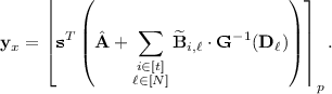
\(\mathsf {TPRF}.\mathsf {ConstrainEval}(\mathsf {pp}, \mathsf {sk}_\mathsf {T}, x)\): On input the public parameters \(\mathsf {pp}\), a constrained key \(\mathsf {sk}_\mathsf {T}= (\mathsf {enc}, \mathsf {ct})\), where \(\mathsf {enc}= \big ( \hat{\mathbf {a}}, \{ \mathbf {a}_b \}_{b \in \{0,1\}}, \{ \mathbf {b}_{i, j} \}_{i\in [t], j\in [z]}, \{ \mathbf {c}_k \}_{k\in [\tau ]} \big )\), \(\mathsf {ct}= \{ \mathsf {ct}_i \}_{i\in [t]}\), and a point \(x \in \{0,1\}^\rho \), the constrained evaluation algorithm computes
$$\begin{aligned} \widetilde{\mathbf {b}}_{i, \ell } \leftarrow \mathsf {Eval}_{\mathsf {ct}}((\mathsf {ct}_i, x), C_{\ell }, \mathbf {b}_{i,1}, \ldots , \mathbf {b}_{i,z}, \mathbf {a}_{x_1}, \ldots , \mathbf {a}_{x_\rho }, \mathbf {c}_1, \ldots , \mathbf {c}_\tau ) \end{aligned}$$for \(i\in [t]\) and \(\ell \in [N]\), and where \(C_\ell (\mathsf {ct}, x) = \mathsf {IP} \circ C_{\mathsf {Eval}}^{(\ell )}\). Then, it computes and outputs the value
-
\(\mathsf {TPRF}.\mathsf {Test}(\mathsf {pp}, \mathsf {tk}, \mathbf {y})\): On input the testing key \(\mathsf {tk}= \{ \mathbf {z}_i \}_{i\in [t]}\) and a point \(\mathbf {y}\in \mathbb {Z}_p^m\), the testing algorithm outputs 1 if \(\left\langle \mathbf {y}, \mathbf {z}_i \right\rangle \in [-B_{\mathsf {test}}, B_{\mathsf {test}}]\) for some \(i\in [t]\) and 0 otherwise.


Correctness Theorem. We now state that under the \(\mathsf {LWE}\) and \(\mathsf {1D\text {-}SIS}\) assumptions (with appropriate parameters), our translucent \(t\)-puncturable PRF \(\varPi _{\mathsf {TPRF}}\) satisfies (selective) evaluation correctness and verification correctness (Definition 4.4, Remark 4.5). We give the formal proof in the full version [34].
Theorem 5.1
(Correctness). Fix a security parameter \(\lambda \), and define parameters \(n, m, p, q, \chi , t, z, \tau , B_{\mathsf {test}}\) as above. Let B be a bound on the error distribution \(\chi \), and suppose \(B_{\mathsf {test}}= B (m + 1)\), \(p = 2^{\rho ^{(1 + \varepsilon )}}\) for some constant \(\varepsilon > 0\), and \(\frac{q}{2 p m B} > B \cdot m^{O(d)}\). Then, take \(m' = m \cdot (3 + t\cdot z+ \tau )\) and \(\beta = B \cdot m^{O(d)}\). Under the \(\mathsf {LWE}_{n, m', q, \chi }\) and \(\mathsf {1D\text {-}SIS\text {-}R}_{m', p, q, \beta }\) assumptions, \(\varPi _{\mathsf {TPRF}}\) is (selectively) correct.
Security Theorems. We now state that under the \(\mathsf {LWE}\) assumption (with appropriate parameters), our translucent \(t\)-puncturable PRF \(\varPi _{\mathsf {TPRF}}\) satisfies selective constrained pseudorandomness (Definition 4.9), selective privacy (Definition 4.12) and weak key-injectivity (Definition 4.14). We give the formal proofs in the full version [34]. As a corollary of satisfying constrained pseudorandomness, we have that \(\varPi _{\mathsf {TPRF}}\) is also pseudorandom (Definition 4.7, Theorem 4.10).
Theorem 5.2
(Constrained Pseudorandomness). Fix a security parameter \(\lambda \), and define parameters \(n, m, p, q, \chi , t, z, \tau \) as above. Let \(m' = m \cdot (3 + t(z+ 1) + \tau )\), \(m'' = m \cdot (3 + t\cdot z+ \tau )\) and \(\beta = B \cdot m^{O(d)}\) where B is a bound on the error distribution \(\chi \). Then, under the \(\mathsf {LWE}_{n, m', q, \chi }\) and \(\mathsf {1D\text {-}SIS\text {-}R}_{m'', p, q, \beta }\) assumptions, \(\varPi _{\mathsf {TPRF}}\) satisfies selective constrained pseudorandomness (Definition 4.9).
Corollary 5.3
(Pseudorandomness). Fix a security parameter \(\lambda \), and define the parameters \(n, m, p, q, \chi , t, z, \tau \) as above. Under the same assumptions as in Theorem 5.2, \(\varPi _{\mathsf {TPRF}}\) satisfies selective pseudorandomness (Definition 4.7).
Theorem 5.4
(Privacy). Fix a security parameter \(\lambda \), and define parameters \(n, m, q, \chi , t, z, \tau \) as above. Let \(m' = m \cdot (3 + t(z+ 1) + \tau )\). Then, under the \(\mathsf {LWE}_{n, m', q, \chi }\) assumption, and assuming the homomorphic encryption scheme \(\varPi _{\mathsf {HE}}\) is semantically secure, \(\varPi _{\mathsf {TPRF}}\) is selectively private (Definition 4.12).
Theorem 5.5
(Key-Injectivity). If the bound B on the error distribution \(\chi \) satisfies \(B < \hat{p} / 2\) where \(\hat{p}\) is the smallest prime dividing the modulus q, and \(m = \omega (n)\), then the translucent \(t\)-puncturable PRF \(\varPi _{\mathsf {TPRF}}\) satisfies key-injectivity (Definition 4.14).
5.2 Concrete Parameter Instantiations
In this section, we give one possible instantiation for the parameters for the translucent \(t\)-puncturable PRF construction in Sect. 5.1. We choose our parameters so that the underlying LWE and 1D-SIS assumptions that we rely on are as hard as approximating worst-case lattice problems to within a subexponential factor \(2^{\tilde{O}(n^{1/c})}\) for some constant c (where n is the lattice dimension). Fix a constant c and a security parameter \(\lambda \).
-
We set the PRF input length \(\rho = \lambda \). Then, the depth \(d_\mathsf {eq}\) of the equality check circuit \(\mathsf {eq}_\ell \) satisfies \(d_\mathsf {eq}= O(\log \rho ) = O(\log \lambda )\).
-
We set the lattice dimension \(n = \lambda ^{2c}\).
-
The noise distribution \(\chi \) is set to be the discrete Gaussian distribution \(D_{\mathbb {Z},\sqrt{n}}\). Then the FHE ciphertext length z and the FHE secret key length \(\tau \) is determined by \(\mathsf {poly}(\lambda , d_\mathsf {eq}, \rho , \log q) = \mathsf {poly}(\lambda )\). The depth of the FHE equality check circuit is \(d = \mathsf {poly}(d_\mathsf {eq},\log z) = \mathsf {polylog}(\lambda )\). Finally, we set \(B_{\mathsf {test}}= B \cdot (m+1)\).
-
We set \(q > m^{O(d)}\) in order to invoke correctness and security of the leveled homomorphic encryption scheme and the matrix embeddings. We refer to the full version [34] for more details. Furthermore, for the 1D-SIS-R assumption, we need q to be the product of \(\lambda \) primes \(p_1, \ldots , p_{\lambda }\). For each \(i \in [\lambda ]\), we set the primes \(p_j= 2^{O(n^{1/2c})}\) such that \(p_1< \cdots < p_{\lambda }\).
-
We set \(p = 2^{n^{1/2c+\varepsilon }}\) for any \(\varepsilon >0\), so the condition in Theorem 5.1 is satisfied.
-
We set \(m = \varTheta (n \log q)\), and \(B_{\mathsf {test}}= B \cdot (m + 1)\). For these parameter settings, \(m^{O(d)} = m^{\mathsf {polylog}(\lambda )}\) and \(q = 2^{\tilde{O}(n^{1/2c})} = 2^{\tilde{O}(\lambda )}\).
Under these parameter setting, the private translucent \(t\)-puncturable PRF in Sect. 5.1 is selectively secure assuming the polynomial hardness of approximating worst-case lattice problems over an n-dimensional lattice to within a subexponential approximation factor \(2^{\tilde{O}(n^{1/2c})}\). Using complexity leveraging [8], the same construction is adaptively secure assuming subexponential hardness of the same worst-case lattice problems.
6 Watermarkable PRFs from Translucent PRFs
In this section, we formally introduce the notion of a watermarkable family of PRFs. Our definitions are adapted from those of [12, 21]. Then, in Sect. 6.2, we show how to construct a secretly-extractable, message-embedding watermarkable family of PRFs from translucent \(t\)-puncturable PRFs. Combined with our concrete instantiation of translucent \(t\)-puncturable PRFs from Sect. 5, this gives the first watermarkable family of PRFs (with security against arbitrary removal strategies) from standard assumptions.
6.1 Watermarking PRFs
We begin by introducing the notion of a watermarkable PRF family.
Definition 6.1
(Watermarkable Family of PRFs [12, adapted]). Fix a security parameter \(\lambda \) and a message space \(\{0,1\}^t\). Then, a secretly-extractable, message-embedding watermarking scheme for a PRF \(\varPi _{\mathsf {PRF}}= (\mathsf {PRF}.\mathsf {KeyGen}, \mathsf {PRF}.\mathsf {Eval})\) is a tuple of algorithms \(\varPi _{\mathsf {WM}}= (\mathsf {WM.Setup}, \mathsf {WM.Mark}, \mathsf {WM.Extract})\) with the following properties:
-
\(\mathsf {WM.Setup}(1^\lambda ) \rightarrow \mathsf {msk}\): On input the security parameter \(\lambda \), the setup algorithm outputs the watermarking secret key \(\mathsf {msk}\).
-
\(\mathsf {WM.Mark}(\mathsf {msk}, k, m) \rightarrow C\): On input the watermarking secret key \(\mathsf {msk}\), a PRF key k (to be marked), and a message \(m \in \{0,1\}^t\), the mark algorithm outputs a marked circuit C.
-
\(\mathsf {WM.Extract}(\mathsf {msk}, C') \rightarrow m\): On input the master secret key \(\mathsf {msk}\) and a circuit \(C'\), the extraction algorithm outputs a string \(m \in \{0,1\}^t\cup \{ \bot \}\).
Definition 6.2
(Circuit Similarity). Fix a circuit class \(\mathcal {C}\) on \(n\)-bit inputs. For two circuits \(C, C' \in \mathcal {C}\) and for a non-decreasing function \(f: \mathbb {N}\rightarrow \mathbb {N}\), we write \(C \sim _fC'\) to denote that the two circuits agree on all but an \(1/f(n)\) fraction of inputs. More formally, we define
We also write \(C \not \sim _fC'\) to denote that C and \(C'\) differ on at least a \(1/f(n)\) fraction of inputs.
Correctness. The correctness property for a watermarking scheme for a PRF family consists of two requirements which we state below.
Definition 6.3
(Watermarking Correctness). Fix a security parameter \(\lambda \). We say that a watermarking scheme \(\varPi _{\mathsf {WM}}= (\mathsf {WM.Setup}, \mathsf {WM.Mark}, \mathsf {WM.Extract})\) for a PRF \(\varPi _{\mathsf {PRF}}= (\mathsf {PRF}.\mathsf {KeyGen}, \mathsf {PRF}.\mathsf {Eval})\) with domain \(\{0,1\}^n\) is correct if for all messages \(m \in \{0,1\}^t\), and setting \(\mathsf {msk}\leftarrow \mathsf {WM.Setup}(1^\lambda )\), \(k \leftarrow \mathsf {PRF}.\mathsf {KeyGen}(1^\lambda )\), and \(C \leftarrow \mathsf {WM.Mark}(\mathsf {msk}, k, m)\), the following two properties hold:
-
Functionality-preserving: \(C(\cdot ) \sim _f\mathsf {PRF}.\mathsf {Eval}(k, \cdot )\) where \(1/f(n) = \mathsf {negl}(\lambda )\) with overwhelming probability.
-
Extraction correctness: \(\Pr [\mathsf {WM.Extract}(\mathsf {msk},C) = m] = 1 - \mathsf {negl}(\lambda )\).
Security. Following [12, 21], we introduce two different security notions for a watermarking scheme: unremovability and unforgeability. We begin by defining the watermarking experiment.
Definition 6.4
(Watermarking Experiment [12, adapted]). Fix a security parameter \(\lambda \). Let \(\varPi _{\mathsf {WM}}= (\mathsf {WM.Setup}, \mathsf {WM.Mark}, \mathsf {WM.Extract})\) be a watermarking scheme for a PRF \(\varPi _{\mathsf {PRF}}= (\mathsf {PRF}.\mathsf {KeyGen}, \mathsf {PRF}.\mathsf {Eval})\) with key-space \(\mathcal {K}\), and let \(\mathcal {A}\) be an adversary. Then the watermarking experiment \(\mathsf {Expt}_{\varPi _{\mathsf {WM}}, \mathcal {A}}(\lambda )\) proceeds as follows. The challenger begins by sampling \(\mathsf {msk}\leftarrow \mathsf {WM.Setup}(1^\lambda )\). The adversary \(\mathcal {A}\) is then given access to the following oracles:
-
Marking oracle. On input a message \(m \in \{0,1\}^t\) and a PRF key \(k \in \mathcal {K}\), the challenger returns the circuit \(C \leftarrow \mathsf {WM.Mark}(\mathsf {msk}, k, m)\) to \(\mathcal {A}\).
-
Challenge oracle. On input a message \(m \in \{0,1\}^t\), the challenger samples a key \(k \leftarrow \mathsf {PRF}.\mathsf {KeyGen}(1^\lambda )\), and returns the circuit \(C \leftarrow \mathsf {WM.Mark}(\mathsf {msk}, k, m)\) to \(\mathcal {A}\).
Finally, \(\mathcal {A}\) outputs a circuit \(C'\). The output of the experiment, denoted \(\mathsf {Expt}_{\varPi _{\mathsf {WM}}, \mathcal {A}}(\lambda )\), is \(\mathsf {WM.Extract}(\mathsf {msk}, C')\).
Definition 6.5
(Unremovability [12, 21]). Fix a security parameter \(\lambda \). For a watermarking scheme \(\varPi _{\mathsf {WM}}= (\mathsf {WM.Setup}, \mathsf {WM.Mark}, \mathsf {WM.Extract})\) for a PRF \(\varPi _{\mathsf {PRF}}= (\mathsf {PRF}.\mathsf {KeyGen}, \mathsf {PRF}.\mathsf {Eval})\) and an adversary \(\mathcal {A}\), we say that \(\mathcal {A}\) is unremoving-admissible if the following conditions hold:
-
The adversary \(\mathcal {A}\) makes exactly one query to the challenge oracle.
-
The circuit \(\tilde{C}\) that \(\mathcal {A}\) outputs satisfies \(\tilde{C} \sim _f\hat{C}\), where \(\hat{C}\) is the circuit output by the challenge oracle and \(1 / f = \mathsf {negl}(\lambda )\).
Then, we say that \(\varPi _{\mathsf {WM}}\) is unremovable if for all efficient and unremoving-admissible adversaries \(\mathcal {A}\),
where \(\hat{m}\) is the message \(\mathcal {A}\) submitted to the challenge oracle in \(\mathsf {Expt}_{\varPi _{\mathsf {WM}}, \mathcal {A}}(\lambda )\).
Definition 6.6
( \(\delta \) -Unforgeability [12, 21]). Fix a security parameter \(\lambda \). For a watermarking scheme \(\varPi _{\mathsf {WM}}= (\mathsf {WM.Setup}, \mathsf {WM.Mark}, \mathsf {WM.Extract})\) for a PRF \(\varPi _{\mathsf {PRF}}= (\mathsf {PRF}.\mathsf {KeyGen}, \mathsf {PRF}.\mathsf {Eval})\) and an adversary \(\mathcal {A}\), we say that \(\mathcal {A}\) is \(\delta \) -unforging-admissible if the following conditions hold:
-
The adversary \(\mathcal {A}\) does not make any challenge oracle queries.
-
The circuit \(\tilde{C}\) that \(\mathcal {A}\) outputs satisfies \(\tilde{C} \not \sim _f C_\ell \) for all \(\ell \in [Q]\), where Q is the number of queries \(\mathcal {A}\) made to the marking oracle, \(C_\ell \) is the output of the marking oracle on the \(\ell ^{\mathrm {th}}\) query, and \(1 / f > \delta \). Moreover, \(\tilde{C} \not \sim _f\mathsf {PRF}.\mathsf {Eval}(k_\ell , \cdot )\), where \(k_\ell \) is the key the adversary submitted on its \(\ell ^{\mathrm {th}}\) query to the marking oracle.
Then, we say that \(\varPi _{\mathsf {WM}}\) is \(\delta \) -unforgeable if for all efficient and \(\delta \)-unforging-admissible adversaries \(\mathcal {A}\),
Remark 6.7
(Giving Access to an Extraction Oracle). As noted in [21], in the secret-key setting, the watermarking security game (Definition 6.4) can be augmented to allow the adversary oracle access to an extraction oracle (which implements \(\mathsf {WM.Extract}(\mathsf {msk}, \cdot )\)). It is an open problem to construct secretly-extractable watermarking from standard assumptions where the adversary is additionally given access to a extraction oracle. The only known constructions today [21] rely on indistinguishability obfuscation.
Remark 6.8
(Marking Oracle Variations). In the watermarking security game (Definition 6.4), the adversary can submit arbitrary keys (of its choosing) to the marking oracle. Cohen et al. [21] also consider a stronger notion where the adversary is allowed to submit arbitrary circuits (not corresponding to any particular PRF) to the marking oracle. However, in this model, they can only achieve lunch-time security (i.e., the adversary can only query the marking oracle before issuing its challenge query). In the model where the adversary can only query the marking oracle on valid PRF keys, their construction achieves full security (assuming the PRF family satisfies a key-injectivity property). Similarly, our construction achieves full security in this model (in the secret-key setting), and also relies on a key-injectivity property on the underlying PRF. Our notion is strictly stronger than the notion in [12]. In the Boneh et al. model [12], the adversary cannot choose the key for the marking oracle. Instead, the marking oracle samples a key (honestly) and gives both the sampled key as well as the watermarked key to the adversary. In contrast, in both our model as well as that in [21], the adversary is allowed to see watermarked keys on arbitrary keys of its choosing. The key difference in our security analysis that enables us to achieve this stronger security notion (compared to [12]) is the new key-injectivity property on the underlying translucent PRF. Instantiating the construction in [12] with a private programmable PRF satisfying key-injectivity should also yield a watermarkable family of PRFs under our strengthened definition.
In the full version of this paper [34], we further compare our correctness and security notions to those considered in previous work [12, 21].
6.2 Watermarking Construction
In this section, we show how any translucent \(t\)-puncturable PRF can be used to obtain a watermarkable family of PRFs. Combined with our construction of a translucent \(t\)-puncturable PRF from Sect. 5.1, we obtain the first watermarkable family of PRFs from standard assumptions.
Construction 6.9
Fix a security parameter \(\lambda \) and a positive real value \(\delta < 1\) such that \(d = \lambda / \delta = \mathsf {poly}(\lambda )\). Let \(\{0,1\}^t\) be the message space for the watermarking scheme. Our construction relies on the following two ingredients:
-
Let \(\varPi _{\mathsf {TPRF}}\) be a translucent \(t\)-puncturable PRF (Definition 4.6) with key-space \(\mathcal {K}\), domain \(\{0,1\}^n\), and range \(\{0,1\}^m\).
-
Let \(\varPi _{\mathsf {PRF}}\) be a secure PRF with domain \((\{0,1\}^m)^d\) and range \((\{0,1\}^n)^{2 t}\).
We require \(n, m, t= \omega (\log \lambda )\). The secretly-extractable, message-embedding watermarking scheme \(\varPi _{\mathsf {WM}}= (\mathsf {WM.Setup}, \mathsf {WM.Mark}, \mathsf {WM.Extract})\) for the PRF associated with \(\varPi _{\mathsf {TPRF}}\) is defined as follows:
-
\(\mathsf {WM.Setup}(1^\lambda )\): On input the security parameter \(\lambda \), the setup algorithm runs \((\mathsf {pp}, \mathsf {tk}) \leftarrow \mathsf {TPRF}.\mathsf {Setup}(1^\lambda )\). Next, for each \(j\in [d]\), it samples \(h_j\overset{\textsc {r}}{\leftarrow }\{0,1\}^n\). It also samples a key \(\mathsf {k}^*\leftarrow \mathsf {PRF}.\mathsf {KeyGen}(1^\lambda )\). Finally, it outputs the master secret key \(\mathsf {msk}= (\mathsf {pp}, \mathsf {tk}, h_1, \ldots , h_d, \mathsf {k}^*)\).
-
\(\mathsf {WM.Mark}(\mathsf {msk}, k, m)\): On input the master secret key \(\mathsf {msk}= (\mathsf {pp}, \mathsf {tk}, h_1, \ldots , h_d, \mathsf {k}^*)\), a PRF key \(k \in \mathcal {K}\) to be marked, and a message \(m \in \{0,1\}^t\), the marking algorithm proceeds as follows:
-
1.
For each \(j\in [d]\), set \(y_j\leftarrow \mathsf {TPRF}.\mathsf {Eval}(\mathsf {pp}, k, h_j)\). Let \(\mathbf {y}= (y_1, \ldots , y_d)\).
-
2.
Compute points \({\mathbf {x}}= \big (x_1^{(0)}, x_1^{(1)}, \ldots , x_t^{(0)}, x_t^{(1)} \big ) \leftarrow \mathsf {PRF}.\mathsf {Eval}(\mathsf {k}^*, \mathbf {y})\).
-
3.
Compute the \(t\)-punctured key \(\mathsf {sk}_S \leftarrow \mathsf {TPRF}.\mathsf {Constrain}(\mathsf {pp}, k, S)\), where the set S is given by \(S = \{ x \in \{0,1\}^n:x \ne x_i^{(m_i)} \ \forall i\in [t] \}\),
-
4.
Output the circuit C where \(C(\cdot ) = \mathsf {TPRF}.\mathsf {ConstrainEval}(\mathsf {pp}, \mathsf {sk}_S, \cdot )\).
-
1.
-
\(\mathsf {WM.Extract}(\mathsf {msk}, C)\): On input the master secret key \(\mathsf {msk}= (\mathsf {pp}, \mathsf {tk}, h_1, \ldots , h_d, k)\) and a circuit \(C : \{0,1\}^n\rightarrow \{0,1\}^m\), the extraction algorithm proceeds as follows:
-
1.
Compute points \({\mathbf {x}}= \big (x_1^{(0)}, x_1^{(1)}, \ldots , x_t^{(0)}, x_t^{(1)} \big ) \leftarrow \mathsf {PRF}.\mathsf {Eval}(\mathsf {k}^*, C(h_1), \ldots , C(h_d))\).
-
2.
For each \(i\in [t]\), and \(b \in \{0,1\}\), compute \(z_i^{(b)} = \mathsf {TPRF}.\mathsf {Test}(\mathsf {pp}, \mathsf {tk}, C(x_i^{(b)}))\).
-
3.
If there exists some \(i\) for which \(z_i^{(0)} = z_i^{(1)}\), output \(\bot \). Otherwise, output the message \(m \in \{0,1\}^t\) where \(m_i= 0\) if \(z_i^{(0)} = 1\) and \(m_i= 1\) if \(z_i^{(1)} = 1\).
-
1.
Security Analysis. We now state the correctness and security theorems for our construction, but defer their formal proofs to the full version of this paper [34].
Theorem 6.10
If \(\varPi _{\mathsf {TPRF}}\) is a secure translucent \(t\)-puncturable PRF, and \(\varPi _{\mathsf {PRF}}\) is a secure PRF, then the watermarking scheme in Construction 6.9 is correct.
Theorem 6.11
If \(\varPi _{\mathsf {TPRF}}\) is a selectively-secure translucent \(t\)-puncturable PRF, and \(\varPi _{\mathsf {PRF}}\) is secure, then the watermarking scheme in Construction 6.9 is unremovable.
Theorem 6.12
If \(\varPi _{\mathsf {TPRF}}\) is a selectively-secure translucent \(t\)-puncturable PRF, and \(\varPi _{\mathsf {PRF}}\) is secure, then the watermarking scheme in Construction 6.9 is \(\delta \)-unforgeable.
Notes
- 1.
There are numerous technicalities in the actual construction, but these are not essential to understanding the main intuition.
- 2.
Another approach for building a watermarkable family of PRFs is to directly construct a private programmable PRF (from standard assumptions) and then invoke the construction in [12]. We discuss this approach at the end of this section.
- 3.
- 4.
- 5.
Since a constrained PRF is a secret-key primitive, we can always include the public parameters as part of the secret key. However, in the lattice-based constrained PRF constructions [3, 10, 17], the public parameters can be sampled once and shared across multiple independent secret keys. Our construction of translucent PRFs will rely on choosing the public parameter matrices to have a certain structure that is shared across multiple secret keys.
- 6.
Normally, multiplication of two inputs requires knowledge of both of the underlying inputs. The “asymmetry” in the embedding scheme of [9] enables multiplications to be done even if only one of the values to be multiplied is known to the evaluator. In the case of computing an inner product between the FHE ciphertext and the FHE secret key, the evaluator knows the bits of the ciphertext, but not the FHE secret key. Thus, the asymmetry enables the evaluator to homomorphically evaluate the inner product without knowledge of the FHE secret key.
- 7.
To actually show that the challenge PRF evaluation is pseudorandom at the punctured point, additional modifications must be made such as introducing extra randomizing terms and collapsing the final PRF evaluation to be field elements instead of vectors. We refer to [10] for the full details.
- 8.
Multiplying by the matrix \(\mathbf {G}^{-1}(\mathbf {D})\) can be viewed as an alternative way to restrict the PRF to the column positions corresponding to the identity submatrix in \(\mathbf {G}\).
- 9.
A similar construction is used in [10] to show security. In their construction, they sample and encrypt a random set of w’s and use them to blind the real PRF value at the punctured point.
- 10.
To reduce notational clutter, we redefine the matrix \(\mathbf {A}_{\mathsf {FHE}, \mathsf {eq}, x}\) here to be the matrix associated with homomorphic evaluation of the scaled equality-check circuit.
- 11.
For the punctured keys to hide the set of punctured points, we need a different trapdoor matrix for each punctured point. We provide the full details in Sect. 5.
- 12.
In the standard constrained pseudorandomness game introduced in [14], the adversary is also allowed to make evaluation queries on values not contained in S. While our construction can be shown to satisfy this stronger property, this is not needed for our watermarking construction. To simplify the presentation and security analysis, we work with this weaker notion here.
- 13.
Roughly speaking, Cohen et al. [21, Definition 7.1] require that for a uniformly random PRF key k, there does not exist a key \(k'\) and a point x where \(\mathsf {PRF}(k, x) = \mathsf {PRF}(k', x)\). In contrast, our notion requires that any two PRF keys do not agree at any particular point with overwhelming probability.
- 14.
For notational convenience, we modify the syntax of the constrain algorithm to take in a set \(\mathsf {T}\) of \(t\) punctured points rather than a set of allowed points.
References
Agrawal, S., Boneh, D., Boyen, X.: Efficient lattice (H)IBE in the standard model. In: Gilbert, H. (ed.) EUROCRYPT 2010. LNCS, vol. 6110, pp. 553–572. Springer, Heidelberg (2010). doi:10.1007/978-3-642-13190-5_28
Agrawal, S., Freeman, D.M., Vaikuntanathan, V.: Functional encryption for inner product predicates from learning with errors. In: Lee, D.H., Wang, X. (eds.) ASIACRYPT 2011. LNCS, vol. 7073, pp. 21–40. Springer, Heidelberg (2011). doi:10.1007/978-3-642-25385-0_2
Banerjee, A., Fuchsbauer, G., Peikert, C., Pietrzak, K., Stevens, S.: Key-homomorphic constrained pseudorandom functions. In: Dodis, Y., Nielsen, J.B. (eds.) TCC 2015. LNCS, vol. 9015, pp. 31–60. Springer, Heidelberg (2015). doi:10.1007/978-3-662-46497-7_2
Banerjee, A., Peikert, C.: New and improved key-homomorphic pseudorandom functions. In: Garay, J.A., Gennaro, R. (eds.) CRYPTO 2014. LNCS, vol. 8616, pp. 353–370. Springer, Heidelberg (2014). doi:10.1007/978-3-662-44371-2_20
Banerjee, A., Peikert, C., Rosen, A.: Pseudorandom functions and lattices. In: Pointcheval, D., Johansson, T. (eds.) EUROCRYPT 2012. LNCS, vol. 7237, pp. 719–737. Springer, Heidelberg (2012). doi:10.1007/978-3-642-29011-4_42
Barak, B., Goldreich, O., Impagliazzo, R., Rudich, S., Sahai, A., Vadhan, S., Yang, K.: On the (im)possibility of obfuscating programs. In: Kilian, J. (ed.) CRYPTO 2001. LNCS, vol. 2139, pp. 1–18. Springer, Heidelberg (2001). doi:10.1007/3-540-44647-8_1
Barak, B., Goldreich, O., Impagliazzo, R., Rudich, S., Sahai, A., Vadhan, S.P., Yang, K.: On the (im)possibility of obfuscating programs. J. ACM 59(2), 6 (2012)
Boneh, D., Boyen, X.: Efficient selective-ID secure identity-based encryption without random oracles. In: Cachin, C., Camenisch, J.L. (eds.) EUROCRYPT 2004. LNCS, vol. 3027, pp. 223–238. Springer, Heidelberg (2004). doi:10.1007/978-3-540-24676-3_14
Boneh, D., Gentry, C., Gorbunov, S., Halevi, S., Nikolaenko, V., Segev, G., Vaikuntanathan, V., Vinayagamurthy, D.: Fully key-homomorphic encryption, arithmetic circuit ABE and compact garbled circuits. In: Nguyen, P.Q., Oswald, E. (eds.) EUROCRYPT 2014. LNCS, vol. 8441, pp. 533–556. Springer, Heidelberg (2014). doi:10.1007/978-3-642-55220-5_30
Boneh, D., Kim, S., Montgomery, H.: Private puncturable PRFs from standard lattice assumptions. In: Coron, J.-S., Nielsen, J.B. (eds.) EUROCRYPT 2017. LNCS, vol. 10210, pp. 415–445. Springer, Cham (2017). doi:10.1007/978-3-319-56620-7_15
Boneh, D., Lewi, K., Montgomery, H., Raghunathan, A.: Key homomorphic PRFs and their applications. In: Canetti, R., Garay, J.A. (eds.) CRYPTO 2013. LNCS, vol. 8042, pp. 410–428. Springer, Heidelberg (2013). doi:10.1007/978-3-642-40041-4_23
Boneh, D., Lewi, K., Wu, D.J.: Constraining pseudorandom functions privately. In: Fehr, S. (ed.) PKC 2017. LNCS, vol. 10175, pp. 494–524. Springer, Heidelberg (2017). doi:10.1007/978-3-662-54388-7_17
Boneh, D., Waters, B.: Conjunctive, subset, and range queries on encrypted data. In: Vadhan, S.P. (ed.) TCC 2007. LNCS, vol. 4392, pp. 535–554. Springer, Heidelberg (2007). doi:10.1007/978-3-540-70936-7_29
Boneh, D., Waters, B.: Constrained pseudorandom functions and their applications. In: Sako, K., Sarkar, P. (eds.) ASIACRYPT 2013. LNCS, vol. 8270, pp. 280–300. Springer, Heidelberg (2013). doi:10.1007/978-3-642-42045-0_15
Boyle, E., Goldwasser, S., Ivan, I.: Functional signatures and pseudorandom functions. In: Krawczyk, H. (ed.) PKC 2014. LNCS, vol. 8383, pp. 501–519. Springer, Heidelberg (2014). doi:10.1007/978-3-642-54631-0_29
Brakerski, Z., Cash, D., Tsabary, R., Wee, H.: Targeted homomorphic attribute-based encryption. In: Hirt, M., Smith, A. (eds.) TCC 2016. LNCS, vol. 9986, pp. 330–360. Springer, Heidelberg (2016). doi:10.1007/978-3-662-53644-5_13
Brakerski, Z., Vaikuntanathan, V.: Constrained key-homomorphic PRFs from standard lattice assumptions. In: Dodis, Y., Nielsen, J.B. (eds.) TCC 2015. LNCS, vol. 9015, pp. 1–30. Springer, Heidelberg (2015). doi:10.1007/978-3-662-46497-7_1
Brakerski, Z., Vaikuntanathan, V.: Circuit-ABE from LWE: unbounded attributes and semi-adaptive security. In: Robshaw, M., Katz, J. (eds.) CRYPTO 2016. LNCS, vol. 9816, pp. 363–384. Springer, Heidelberg (2016). doi:10.1007/978-3-662-53015-3_13
Canetti, R., Chen, Y.: Constraint-hiding constrained PRFs for NC\({}^{\text{1}}\) from LWE. In: EUROCRYPT (2017)
Canetti, R., Dwork, C., Naor, M., Ostrovsky, R.: Deniable encryption. In: Kaliski, B.S. (ed.) CRYPTO 1997. LNCS, vol. 1294, pp. 90–104. Springer, Heidelberg (1997). doi:10.1007/BFb0052229
Cohen, A., Holmgren, J., Nishimaki, R., Vaikuntanathan, V., Wichs, D.: Watermarking cryptographic capabilities. In: STOC (2016)
Cox, I., Miller, M., Bloom, J., Fridrich, J., Kalker, T.: Digital Watermarking and Steganography. Morgan Kaufmann, Burlington (2007)
Garg, S., Gentry, C., Halevi, S., Raykova, M., Sahai, A., Waters, B.: Candidate indistinguishability obfuscation and functional encryption for all circuits. In: FOCS (2013)
Gay, R., Méaux, P., Wee, H.: Predicate encryption for multi-dimensional range queries from lattices. In: Katz, J. (ed.) PKC 2015. LNCS, vol. 9020, pp. 752–776. Springer, Heidelberg (2015). doi:10.1007/978-3-662-46447-2_34
Gentry, C.: Fully homomorphic encryption using ideal lattices. In: STOC (2009)
Gentry, C., Gorbunov, S., Halevi, S.: Graph-induced multilinear maps from lattices. In: Dodis, Y., Nielsen, J.B. (eds.) TCC 2015. LNCS, vol. 9015, pp. 498–527. Springer, Heidelberg (2015). doi:10.1007/978-3-662-46497-7_20
Gentry, C., Sahai, A., Waters, B.: Homomorphic encryption from learning with errors: conceptually-simpler, asymptotically-faster, attribute-based. In: Canetti, R., Garay, J.A. (eds.) CRYPTO 2013. LNCS, vol. 8042, pp. 75–92. Springer, Heidelberg (2013). doi:10.1007/978-3-642-40041-4_5
Gorbunov, S., Vaikuntanathan, V., Wee, H.: Attribute-based encryption for circuits. In: STOC (2013)
Gorbunov, S., Vaikuntanathan, V., Wee, H.: Predicate encryption for circuits from LWE. In: Gennaro, R., Robshaw, M. (eds.) CRYPTO 2015. LNCS, vol. 9216, pp. 503–523. Springer, Heidelberg (2015). doi:10.1007/978-3-662-48000-7_25
Gorbunov, S., Vinayagamurthy, D.: Riding on asymmetry: efficient ABE for branching programs. In: Iwata, T., Cheon, J.H. (eds.) ASIACRYPT 2015. LNCS, vol. 9452, pp. 550–574. Springer, Heidelberg (2015). doi:10.1007/978-3-662-48797-6_23
Hopper, N., Molnar, D., Wagner, D.: From weak to strong watermarking. In: Vadhan, S.P. (ed.) TCC 2007. LNCS, vol. 4392, pp. 362–382. Springer, Heidelberg (2007). doi:10.1007/978-3-540-70936-7_20
Katz, J., Sahai, A., Waters, B.: Predicate encryption supporting disjunctions, polynomial equations, and inner products. In: Smart, N. (ed.) EUROCRYPT 2008. LNCS, vol. 4965, pp. 146–162. Springer, Heidelberg (2008). doi:10.1007/978-3-540-78967-3_9
Kiayias, A., Papadopoulos, S., Triandopoulos, N., Zacharias, T.: Delegatable pseudorandom functions and applications. In: CCS (2013)
Kim, S., Wu, D.J.: Watermarking cryptographic functionalities from standard lattice assumptions. IACR Cryptology ePrint Archive 2017 (2017)
Naccache, D., Shamir, A., Stern, J.P.: How to copyright a function? In: Imai, H., Zheng, Y. (eds.) PKC 1999. LNCS, vol. 1560, pp. 188–196. Springer, Heidelberg (1999). doi:10.1007/3-540-49162-7_14
Nishimaki, R.: How to watermark cryptographic functions. In: Johansson, T., Nguyen, P.Q. (eds.) EUROCRYPT 2013. LNCS, vol. 7881, pp. 111–125. Springer, Heidelberg (2013). doi:10.1007/978-3-642-38348-9_7
Nishimaki, R., Wichs, D., Zhandry, M.: Anonymous traitor tracing: how to embed arbitrary information in a key. In: Fischlin, M., Coron, J.-S. (eds.) EUROCRYPT 2016. LNCS, vol. 9666, pp. 388–419. Springer, Heidelberg (2016). doi:10.1007/978-3-662-49896-5_14
Regev, O.: On lattices, learning with errors, random linear codes, and cryptography. In: STOC (2005)
Sahai, A., Waters, B.: Fuzzy identity-based encryption. In: Cramer, R. (ed.) EUROCRYPT 2005. LNCS, vol. 3494, pp. 457–473. Springer, Heidelberg (2005). doi:10.1007/11426639_27
Yoshida, M., Fujiwara, T.: Toward digital watermarking for cryptographic data. IEICE Trans. 94–A(1), 270–272 (2011)
Acknowledgments
We thank Vinod Vaikuntanathan and Daniel Wichs for pointing out the connection between private programmable PRFs and private puncturable PRFs. We thank Yilei Chen for many helpful discussions about watermarking. This work was funded by NSF, DARPA, a grant from ONR, and the Simons Foundation. Opinions, findings and conclusions or recommendations expressed in this material are those of the authors and do not necessarily reflect the views of DARPA.
Author information
Authors and Affiliations
Corresponding author
Editor information
Editors and Affiliations
Rights and permissions
Copyright information
© 2017 International Association for Cryptologic Research
About this paper
Cite this paper
Kim, S., Wu, D.J. (2017). Watermarking Cryptographic Functionalities from Standard Lattice Assumptions. In: Katz, J., Shacham, H. (eds) Advances in Cryptology – CRYPTO 2017. CRYPTO 2017. Lecture Notes in Computer Science(), vol 10401. Springer, Cham. https://doi.org/10.1007/978-3-319-63688-7_17
Download citation
DOI: https://doi.org/10.1007/978-3-319-63688-7_17
Published:
Publisher Name: Springer, Cham
Print ISBN: 978-3-319-63687-0
Online ISBN: 978-3-319-63688-7
eBook Packages: Computer ScienceComputer Science (R0)
