Propagation Modeling

Abstract

The design of spectrally efficient wireless communication systems requires a thorough understanding of the radio propagation channel. This chapter emphasizes land mobile radio channels, including those found in cellular land mobile radio systems and mobile ad hoc networks including vehicle-to-vehicle channels. The chapter first treats the characteristics of the complex faded envelope in frequency non-selective (flat) fixed-to-mobile channels that are typically found in cellular land mobile radio systems, including the received envelope and phase distribution, envelope correlation and spectra, level crossing rates and fade durations, and space-time correlation. Afterwards, mobile-to-mobile channels are considered. This is followed by a statistical characterization of frequency-selective fading channels, and treatment of polarized fading channels. The chapter continues with a discussion of simulation techniques for fading channels, including filtered white noise, sum of sinusoid techniques such as the classical Jakes’ technique, and techniques for generating multiple uncorrelated faded envelopes. Advanced simulation methodologies are discussed including wide-band simulation models such as the COST207 and COST259 models, symbol-spaced simulation models, and mobile-to-mobile simulation models. The chapter goes on to discuss modeling and simulation techniques for long term fading or shadowing. Finally, the chapter wraps up with theoretical and empirical path loss models, including the famous Okumura–Hata model, Lee’s model, various COST models, and 3GPP mm-wave path loss models.

Appendices

Appendix 2A: COST 207 Channel Models

The COST 207 study has specified typical realizations for the power-delay profile in the following environments; Typical Urban (TU), Bad Urban (BA), Reduced TU, Reduced BU, Rural Area (RA), and Hilly Terrain (HT) [79]. The models below are identical to the COST 207 models, except that fractional powers have been normalized so as to sum to unity, i.e., the envelope power is normalized to unity.

Table 2.7 COST 207 Typical Urban (TU) (σ _τ  = 1. 0 μs) and Bad Urban (BU) (σ _τ  = 2. 5 μs) power-delay profiles, from [79]

Table 2.8 COST 207 Reduced Typical Urban (TU) (σ _τ  = 1. 0 μs) and Reduced Bad Urban (BU) (σ _τ  = 2. 5 μs) power-delay profiles, from [79]

Table 2.9 COST 207 Typical Rural (non-hilly) Area (RA) power-delay profile (σ _τ  = 0. 1 μs), from [79]

Table 2.10 COST 207 Typical Hilly Terrain (HT) power-delay profile (σ _τ  = 5. 0 μs), from [79]

Table 2.11 COST 207 Reduced Hilly Terrain (HT) power-delay profile (σ _τ  = 5. 0 μs), from [79]

Appendix 2B: COST 259 Channel Models

The 3GPP standards group has defined three typical realizations for the COST 259 models; Typical Urban (TUx), Rural Area (RAx), and Hilly Terrain (HTx), where x is the MS speed in km/h, [113]. Default speeds are 3, 50, and 120 km/h for the TUx model, 120 and 250 km/h for the RAx model, and 120 km/h for the HTx model.

Table 2.12 COST 259 Typical Urban (TUx) channel model, from [113]

Table 2.13 COST 259 Rural Area (RAx) channel model, from [113]

Appendix 2C: ITU Channel Models

ITU models have been developed indoor office, outdoor to indoor and pedestrian, and vehicular-high antenna [276]. The models below are identical to the ITU models, except that fractional powers have been normalized so as to sum to unity, i.e., the envelope power is normalized to unity.

Table 2.14 COST 259 Hilly Terrain (HTx) channel model, from [113]

Table 2.15 ITU indoor office environment power-delay profiles, from [276]

Table 2.16 ITU outdoor to indoor and pedestrian power-delay profiles, from [276]

Table 2.17 ITU vehicular power-delay profiles, from [276]

Appendix 2D: Derivation of Eq. (2.358)

This Appendix derives an expression for the second moment of a Ricean random variable in terms of its first moment. A Ricean random variable X has probability density function, cf., (2.57)

$$\displaystyle{ p_{X}(x) = \frac{x} {b_{0}}\exp \left \{-\frac{x^{2} + s^{2}} {2b_{0}} \right \}I_{0}\left (\frac{xs} {b_{0}} \right )\ \ \ x> 0 }$$

(2D.1)

and moments [272]

$$\displaystyle{ \mathrm{E}[X^{n}] = (2b_{ 0})^{\frac{n} {2} }\exp \left \{-\frac{s^{2}} {2b_{0}}\right \}\Gamma \left (\frac{} {}(2 + n)/2\right )\ _{1}\mathrm{F}_{1}\left (\frac{n + 2} {2},1; \frac{s^{2}} {2b_{0}}\right ) }$$

(2D.2)

where $\Gamma (\ \cdot \ )$ is the Gamma function, and₁F₁(a, b; x) is the confluent hypergeometric function. The first moment of X is

$$\displaystyle{ \mathrm{E}[X] \equiv \varOmega _{v} = (2b_{0})^{\frac{1} {2} }\mathrm{e}^{-K}\frac{\sqrt{\pi }} {2} \ _{1}\mathrm{F}_{1}(3/2,1;K), }$$

(2D.3)

where K = s ²∕2b ₀ is the Rice factor. The second moment of X is

$$\displaystyle\begin{array}{rcl} \mathrm{E}[X^{2}] \equiv \varOmega _{ p}& =& 2b_{0}\mathrm{e}^{-K}\ _{ 1}\mathrm{F}_{1}(2,1;K) \\ & =& 2b_{0}(K + 1). {}\end{array}$$

(2D.4)

Substituting 2b ₀ from (2D.3) into (2D.4) gives

$$\displaystyle{ \varOmega _{p} = \frac{4\mathrm{e}^{2K}\ (K + 1)} {\pi \ _{1}\mathrm{F}_{1}^{2}(3/2,1;K)}\ \varOmega _{v}^{2} = C(K)\ \varOmega _{ v}^{2}. }$$

(2D.5)

Note that C(0) = 4∕π, C(∞) = 1, and 4∕π ≤ C(K) ≤ 1 for 0 ≤ K ≤ ∞.

Appendix 2E: Derivation of Eq. (2.374)

From (2.373), the composite distribution for the squared-envelope, α _c ², is

$$\displaystyle\begin{array}{rcl} p_{\alpha _{c}^{2}}(x)& =& \int _{0}^{\infty }\left (\frac{m} {w}\right )^{m}\frac{x^{m-1}} {\Gamma (m)}\exp \left \{-\frac{mx} {w} \right \} \frac{1} {\sqrt{2\pi }\xi \sigma _{\varOmega }w}\exp \left \{-\frac{(10\mathrm{log}_{10}\{w\} -\mu _{\varOmega _{p\ \mathrm{(dB)}}})^{2}} {2\sigma _{\varOmega }^{2}} \right \}\mathrm{d}w,{}\end{array}$$

(2E.1)

where ξ = ln(10)∕10. The mean of the approximate log-normal distribution is

$$\displaystyle\begin{array}{rcl} \mu _{\mathrm{(dBm)}}& =& \mathrm{E}[10\mathrm{log}_{10}\{\alpha _{c}^{2}\}] \\ & =& \int _{0}^{\infty }\int _{ 0}^{\infty }10\mathrm{log}_{ 10}\{x\}\left (\frac{m} {w}\right )^{m}\frac{x^{m-1}} {\Gamma (m)}\exp \left \{-\frac{mx} {w} \right \} \frac{1} {\sqrt{2\pi }\xi \sigma _{\varOmega }w}\exp \left \{-\frac{(10\mathrm{log}_{10}\{w\} -\mu _{\varOmega _{p\ \mathrm{(dB)}}})^{2}} {2\sigma _{\varOmega }^{2}} \right \}\mathrm{d}w\mathrm{d}x \\ & =& \frac{10m^{m}} {\sqrt{2\pi }\xi \sigma _{\varOmega }\Gamma (m)}\int _{0}^{\infty } \frac{1} {w^{m+1}}\exp \left \{-\frac{(10\mathrm{log}_{10}\{w\} -\mu _{\varOmega _{p\ \mathrm{(dB)}}})^{2}} {2\sigma _{\varOmega }^{2}} \right \}\int _{0}^{\infty }\mathrm{log}_{ 10}\{x\}\ x^{m-1}\exp \left \{-\frac{mx} {w} \right \}\mathrm{d}x\mathrm{d}w.{}\end{array}$$

(2E.2)

Assuming that m is an integer, the inner integral becomes [147, 4.352.2]

$$\displaystyle{ \int _{0}^{\infty }\mathrm{log}_{ 10}\{x\}x^{m-1}\exp \left \{-\frac{mx} {w} \right \}\mathrm{d}x = \frac{\Gamma (m)w^{m}} {m^{m}\ln 10} \left (\psi (m) -\ln (m/w)\right ). }$$

(2E.3)

Then by using the change of variables x = 10log₁₀{w},

$$\displaystyle{ \mu _{\mathrm{(dBm)}} =\xi ^{-1}\left (\psi (m) -\ln (m)\right ) +\mu _{\varOmega _{ p\ \mathrm{(dB)}}}, }$$

(2E.4)

where ψ( ⋅ ) is the Euler psi function, and

$$\displaystyle{ \psi (m) = -C +\sum _{ k=1}^{m-1} \frac{1} {k} }$$

(2E.5)

and C ≃ 0. 5772 is Euler’s constant. Likewise, the second moment of the approximate log-normal distribution is

$$\displaystyle\begin{array}{rcl} \mathrm{E}[(10\mathrm{log}_{10}(\alpha _{c}^{2}))^{2}]& =& \int _{ 0}^{\infty }\int _{ 0}^{\infty }\left (10\mathrm{log}_{ 10}\{x\}\right )^{2}\left (\frac{m} {w}\right )^{m}\frac{x^{m-1}} {\Gamma (m)}\exp \left \{-\frac{mx} {w} \right \} \frac{1} {\sqrt{2\pi }\xi \sigma _{\varOmega }w}\exp \left \{-\frac{(10\mathrm{log}_{10}\{w\} -\mu _{\varOmega _{p\mathrm{(dB)}}})^{2}} {2\sigma _{\varOmega }^{2}} \right \}\mathrm{d}w\mathrm{d}x \\ & =& \frac{m^{m}} {\sqrt{2\pi }\xi \Gamma (m)}\int _{0}^{\infty } \frac{1} {w^{m+1}}\exp \left \{-\frac{(10\log _{10}\{w\} -\mu _{\varOmega _{p\ \mathrm{(dB)}}})^{2}} {2\sigma _{\varOmega }^{2}} \right \}\int _{0}^{\infty }\left (10\mathrm{log}_{ 10}\{x\}\right )^{2}x^{m-1}\exp \left \{-\frac{mx} {w} \right \}\mathrm{d}x\mathrm{d}w.{}\end{array}$$

(2E.6)

Assuming again that m is an integer, the inner integral is [147, 4.358.2]

$$\displaystyle\begin{array}{rcl} \int _{0}^{\infty }\left (10\mathrm{log}_{ 10}(x)\right )^{2}x^{m-1}\exp \left \{-\frac{mx} {w} \right \}\mathrm{d}x& =& \frac{(m - 1)!w^{m}} {m^{m}\ln 10} \left (\left (\psi (m) -\ln (m/w)\right )^{2} +\zeta (2,m)\right ) {}\\ \end{array}$$

leading to

$$\displaystyle\begin{array}{rcl} \mathrm{E}[(10\mathrm{log}_{10}\{\alpha _{c}^{2}\})^{2}]& =& \zeta ^{2}\left (\left (\psi (m) -\ln (m)\right )^{2}\mu _{ \varOmega _{p\ \mathrm{(dB)}}}^{2} +\zeta (2,m)\right ) + 2\zeta \left (\psi (m) -\ln (m)\right )\mu _{\varOmega _{ p\ \mathrm{(dB)}}} +\sigma ^{2} +\mu _{ \varOmega _{ p\ \mathrm{(dB)}}}^{2},{}\end{array}$$

(2E.7)

where

$$\displaystyle{ \zeta (2,m) =\sum _{ k=0}^{\infty } \frac{1} {(m + k)^{2}} }$$

(2E.8)

is Reimann’s zeta function. Finally, the variance of the approximate log-normal distribution is

$$\displaystyle\begin{array}{rcl} \sigma ^{2}& =& \mathrm{E}[(10\mathrm{log}_{ 10}\{\alpha _{c}^{2}\})^{2}] -\mathrm{ E}^{2}[10\mathrm{log}_{ 10}\{\alpha _{c}^{2}\}] \\ & =& \xi ^{-2}\zeta (2,m) +\sigma _{ \varOmega }^{2}. {}\end{array}$$

(2E.9)

Problems

2.1. Suppose that r(t) is a wide-sense stationary (WSS) bandpass random process, such that

$$\displaystyle{r(t) = g_{I}(t)\cos (2\pi f_{c}t) - g_{Q}(t)\sin (2\pi f_{c}t)}$$

• (a) Show that the auto- and cross-correlations of g _I (t) and g _Q (t) must satisfy the following conditions:

  $$\displaystyle\begin{array}{rcl} \phi _{g_{I}g_{I}}(\tau )& =& \phi _{g_{Q}g_{Q}}(\tau ) {}\\ \phi _{g_{I}g_{Q}}(\tau )& =& -\phi _{g_{Q}g_{I}}(\tau ) {}\\ \end{array}$$

• (b) Under the conditions in part a) show that the autocorrelation of r(t) is

  $$\displaystyle{\mathrm{E}[r(t)r(t+\tau )] =\phi _{g_{I}g_{I}}(\tau )\cos (2\pi f_{c}\tau ) -\phi _{g_{I}g_{Q}}(\tau )\sin (2\pi f_{c}\tau ).}$$

2.2. What is the maximum Doppler shift for the GSM mobile cellular system on the “downlink” from the base station to the mobile unit (935–960 MHz RF band)? What is it on the “uplink” direction, or mobile to base (890–915 MHz RF band)? Assume a high-speed train traveling at a speed of v = 250 km/h.

2.3. This problem considers two ray channels exhibiting either frequency selective or time selective behavior.

• (a) Consider the transmission of a bandpass signal having complex envelope $\tilde{s}(t)$ on a channel such that the received complex envelope is

  $$\displaystyle{\tilde{r}(t) =\alpha \tilde{ s}(t) +\beta \tilde{ s}(t -\tau _{1}),}$$

  where α and β are real valued.

  • i) Find the channel impulse response g(t, τ).

  • ii) Find the channel magnitude response | G(t, f) | .

  • iii) Find the channel phase response ∠ G(t, f).

• (b) Consider the transmission of a bandpass signal having complex envelope $\tilde{s}(t)$ on a channel such that the received complex envelope is

  $$\displaystyle{\tilde{r}(t) =\alpha \tilde{ s}(t) +\beta \tilde{ s}(t)\mathrm{e}^{j2\pi f_{d}t},}$$

  where α and β are real valued.

  • i) Find the channel impulse response g(t, τ).

  • ii) Find the channel magnitude response | G(t, f) | .

  • iii) Find the channel phase response ∠ G(t, f).

2.4. A wireless channel is characterized by the time-variant impulse response

$$\displaystyle{g(t,\tau ) = \left (1 - \frac{\tau } {T}\right )\cos \left (\varOmega t +\phi _{0}\right ),\ \ \ \ 0 \leq \tau \leq T\,}$$

where T = 0. 05 ms, Ω = 10π, and ϕ ₀ ∈ (−π, +π] is a constant.

• (a) Determine the channel time-variant transfer function.

• (b) Given an input signal having the complex envelope

  $$\displaystyle{\tilde{s}(t) = \left \{\begin{array}{ll} 1,&\ \ 0 \leq t \leq T_{s} \\ 0,&\ \ \mbox{ otherwise}\end{array} \right.\,}$$

  determine the complex envelope of the signal at the output of the channel, $\tilde{r}(t)$. Make sure to consider cases when 0 < T _s  < T and 0 < T < T _s , separately.

• (c) Consider digital modulation scheme with a modulated symbol interval T _s . If the channel fading is frequency selective, specify the relation between T _s and T.

2.5. Suppose that an omnidirectional antenna is used and the azimuth angle-of-arrival distribution, p(θ), is given by (2.52). Find the Doppler power spectrum S _gg (f).

2.6. A very useful model for a non-isotropic scattering environment assumes that the azimuth angle-of-arrival distribution is described by the von Mises pdf in (2.51).

• (a) Assuming an isotropic receiver antenna, calculate the received Doppler power spectrum, S _gg (f).

• (b) Under what conditions are the quadrature components g _I (t) and g _Q (t) uncorrelated?

2.7. Determine and plot the (normalized) power spectral densities S _gg (f) for the following cases. Assume 2-D isotropic scattering;

• (a) A vertical loop antenna in the plane perpendicular to vehicle motion, $G(\theta ) = \frac{3} {2}\sin ^{2}(\theta )$.

• (b) A vertical loop antenna in the plane of vehicle motion, $G(\theta ) = \frac{3} {2}\cos ^{2}(\theta )$.

• (c) A directional antenna of beamwidth β directed perpendicular to vehicle motion with (see Fig. 2.70a)

  $$\displaystyle{G(\theta ) = \left \{\begin{array}{cc} G_{0}\,&\vert \frac{\pi }{2} -\theta \vert <\beta /2 \\ 0\, &\mbox{ otherwise}\end{array} \right..}$$

  Fig. 2.70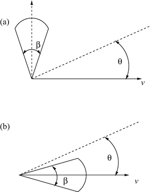

  

  Scenario for Problem 2.7 parts (a ) and (b )

• (d) A directional antenna of beamwidth β directed along vehicle motion with (see Fig. 2.70b)

  $$\displaystyle{G(\theta ) = \left \{\begin{array}{cc} G_{0}\,& \vert \theta \vert <\beta /2 \\ 0\, &\mbox{ otherwise}\end{array} \right..}$$

2.8. Consider a narrow-band channel with a 700 MHz carrier frequency. The complex channel gain at a mobile station is g(t) = g _I (t) + jg _Q (t), such that

$$\displaystyle\begin{array}{rcl} S_{g_{I}g_{I}}(f)& =& \left \{\begin{array}{ll} \mathrm{rect}\left ( \frac{f} {200}\right ),&\ \ \ \ \vert f\vert \leq 100\,\text{Hz}\\ 0, &\ \ \ \ \mathrm{elsewhere } \end{array} \right. {}\\ S_{g_{I}g_{Q}}(f)& =& 0. {}\\ \end{array}$$

• (a) What is the speed of the mobile station?

• (b) What is the cross-correlation function $\phi _{g_{I}g_{Q}}(\tau )$ of the I and Q components of the faded envelope?

• (c) If antenna diversity is deployed at the mobile station, what are the possible spatial separations between the antenna elements such that the corresponding faded envelopes will be uncorrelated?

• (d) Write down an expression for $\phi _{g_{Q}g_{Q}}(\tau )$.

2.9. Consider a Ricean fading channel with Rice factor K and average envelope power Ω _p . Assume that the means m _I (t) and m _Q (t) of the in-phase and quadrature components are given by (2.59) and (2.60), respectively. Derive an integral expression for the probability density function of the envelope phase in terms of K and Ω _p .

2.10. Consider a 2-D isotropic scattering channel. Show that the psd of the received envelope α(t) = | g(t) | is given by (2.77).

2.11. Suppose that the Doppler spectrum is given by

$$\displaystyle{S_{gg}(f) = A\mathrm{rect}\left (\frac{f + f_{1}} {W_{d}} \right ) + A\mathrm{rect}\left (\frac{f - f_{1}} {W_{d}} \right )}$$

where

$$\displaystyle{\mathrm{rect}\left ( \frac{f} {W_{d}}\right ) = \left \{\begin{array}{ll} 1&\,\ \ \ \vert f\vert \leq W_{d}/2 \\ 0&\,\ \ \ \mathrm{elsewhere} \end{array} \right.}$$

and A, f ₁, and W _d are constants.

• (a) Sketch the Doppler spectrum.

• (b) Find the envelope correlation function

  $$\displaystyle{\phi _{gg}(\tau ) =\phi _{g_{I}g_{I}}(\tau ) + j\phi _{g_{I}g_{Q}}(\tau )}$$

• (c) For which values of τ are g(t) and g(t +τ) uncorrelated?

2.12. Suppose that the Doppler power spectrum is given by the following function:

$$\displaystyle{S_{gg}(f) = A\cos \left ( \frac{\pi f} {2f_{m}}\right )\mathrm{rect}\left ( \frac{f} {2f_{m}}\right )}$$

• (a) Find the corresponding envelope autocorrelation function ϕ _gg (τ).

• (b) For what values of τ are g _I (t) and g _Q (t +τ) uncorrelated?

• (c) Given that

  $$\displaystyle{\varOmega _{p} =\phi _{gg}(0) =\int _{ -f_{m}}^{f_{m} }S_{gg}(f)df}$$

  find the value of A in terms of Ω _p .

2.13. Consider the non-isotropic scattering environment shown in Fig. 2.7. Show that the continuous portion of the psd of the received envelope α(t) = | g(t) | is given by (2.79).

2.14. Consider a wide-sense stationary zero-mean complex Gaussian random process g(t) having the autocorrelation function $\phi _{gg}(\tau ) =\phi _{g_{I}g_{I}}(\tau ) + j\phi _{g_{I}g_{Q}}(\tau )$. Show that the autocorrelation and autocovariance functions of the squared-envelope α ²(t) = | g(t) | ² are given by (2.82) and (2.83), respectively.

2.15. Consider a wide-sense stationary non-zero-mean complex Gaussian random process g(t) = g _I (t) + jg _Q (t), where

$$\displaystyle\begin{array}{rcl} g_{I}(t)& =& \hat{g}_{I}(t) + m_{I}(t) {}\\ g_{Q}(t)& =& \hat{g}_{Q}(t) + m_{Q}(t) {}\\ \end{array}$$

and m _I (t) and m _Q (t) are the means of g _I (t) and g _Q (t), respectively. Show that the autocorrelation and autocovariance functions of the squared-envelope α ²(t) = | g(t) | ² are given by (2.87) and (2.90), respectively.

2.16. Establish the equivalence between (2.102) and (2.103).

2.17. A flat Rayleigh fading signal at 6 GHz is received by a vehicle traveling at 80 km/hr.

• (a) Determine the number of positive-slope zero crossings of the rms envelope level that occur over a 5 s interval.

• (b) Determine the average duration of a fade below the rms envelope level.

• (c) Determine the average duration of a fade at a level of 20 dB below the rms envelope level.

2.18. Consider a situation where the received envelope is Rayleigh faded (K = 0), but the Doppler power spectrum S _gg ^c(f) is not symmetrical about f = 0, i.e., a form of non-isotropic scattering. Show that the envelope level crossing rate is given by

$$\displaystyle{L_{R} = \sqrt{\frac{b_{2 } } {b_{0}} -\frac{b_{1}^{2}} {b_{0}^{2}}} \cdot \frac{\rho } {\sqrt{\pi }}\mathrm{e}^{-\rho ^{2} },}$$

where

$$\displaystyle{\rho = \frac{R} {\sqrt{\varOmega _{p}}} = \frac{R} {\sqrt{2b_{0}}}.}$$

and the b _i are defined in (2.102) with f _q  = 0.

2.19. Consider the situation in Fig. 2.71, where the mobile station employs a directional antenna with a beam width of ϕ ^∘. Assume a 2-D isotropic scattering environment.

Fig. 2.71

Mobile with directional antenna for Problem 2.19

• (a) In receiving a radio transmission at 850 MHz, a Doppler frequency of 20–60 Hz is observed. What is the beam width of the mobile station antenna, and how fast is the mobile station traveling?

• (b) Suppose that the mobile station antenna has a beam width of 13^∘. What is the level crossing rate with respect to the rms envelope level, assuming that the mobile station is traveling at a speed of 30 km/h?

2.20. Consider a cellular radio system with fixed base stations and moving mobile stations. The channel is characterized by flat Rayleigh fading channel with two-dimensional isotropic scattering. The mobile station employs omni-directional antennas and the system operates at an RF carrier frequency of 900 MHz.

• (a) Determine the positive going level crossing rate at the normalized envelope level ρ = 1, when the maximum Doppler frequency is f _m  = 20 Hz. Compute the velocity of the mobile station.

• (b) Now suppose that the mobile station is travelling at a speed of 24 km/h. Calculate the average fade duration (AFD) and level crossing rate (LCR) at the normalized envelope level ρ = 0. 294.

2.21. A vehicle experiences 2-D isotropic scattering and receives a Rayleigh faded 900 MHz signal while traveling at a constant velocity for 10 s. Assume that the local mean remains constant during travel, and the average duration of fades 10 dB below the rms envelope level is 1 ms.

• (a) How far does the vehicle travel during the 10 s interval?

• (b) How many fades is the envelope expected to undergo that are 10 dB below the rms envelope level during the 10 s interval?

2.22. A vehicle receives a Ricean faded signal where the specular component is at the frequency f _c and scatter component is due to 2-D isotropic scattering.

• (a) Compute the average duration of fades that 10 dB below the rms envelope level for K = 0, 7, 20, and a maximum Doppler frequency of f _m  = 20 Hz.

• (b) Suppose that data is transmitted using binary modulation at a rate of 1 Mbps, and an envelope level that is 10 dB below the rms envelope level represents a threshold between “error-free” and “error-prone” conditions. During error-prone conditions, bits are in error with probability one-half. Assuming that the data is transmitted in 10,000-bit packets, how many bits errors (on the average) will each transmitted packet contain?

2.23. Show that for wide-sense stationary (WSS) channels

$$\displaystyle\begin{array}{rcl} \phi _{H}(f,m;\nu,\mu )& =& \psi _{H}(f,m;\nu )\delta (\nu -\mu ) {}\\ \phi _{S}(\tau,\eta;\nu,\mu )& =& \psi _{S}(\tau,\eta;\nu )\delta (\nu -\mu ). {}\\ \end{array}$$

That is, the channel correlation functions ϕ _H (f, m; ν, μ) and ϕ _S (τ, η; ν, μ) have a singular behavior with respect to the Doppler shift variable. What is the physical interpretation of this property?

2.24. Show that for uncorrelated scattering (US) channels

$$\displaystyle\begin{array}{rcl} \phi _{g}(t,s;\tau,\eta )& =& \psi _{g}(t,s;\tau )\delta (\eta -\tau ) {}\\ \phi _{S}(\tau,\eta;\nu,\mu )& =& \psi _{S}(\tau;\nu,\mu )\delta (\eta -\tau ). {}\\ \end{array}$$

That is, the channel correlation functions ϕ _g (t, s; τ, η) and ϕ _S (τ, η; ν, μ) have a singular behavior with respect to the time delay variable. What is the physical interpretation of this property?

2.25. Given the channel input signal $\tilde{s}(t)$ and the channel delay-Doppler spread function S(τ, ν), show that the channel output signal is

$$\displaystyle{\tilde{r}(t) =\int _{ -\infty }^{\infty }\int _{ -\infty }^{\infty }\tilde{s}(t-\tau )S(\tau,\nu )\mathrm{e}^{-j2\pi f\tau }\mathrm{d}\nu \mathrm{d}\tau.}$$

How do you interpret the channel function S(τ, ν)?

2.26. Suppose that the spaced-time spaced-frequency correlation function of a WSSUS channel has the following form

$$\displaystyle{\phi _{T}(\varDelta f;\varDelta t) =\exp \left \{-b\vert \varDelta t\vert \right \} \frac{1} {a + j2\pi \varDelta f}.}$$

• (a) Find the corresponding channel correlation function ψ _g (Δ t; τ).

• (b) Find the corresponding scattering function ψ _S (ν; τ).

• (c) What is the average delay spread, μ _τ , and rms delay spread σ _τ ?

2.27. The scattering function for a WSSUS scattering channel is given by

$$\displaystyle{\psi _{S}(\tau,\nu ) =\varOmega _{p} \cdot \frac{2a} {a^{2} + (2\pi \nu )^{2}} \cdot be^{-b\tau }u(\tau ).}$$

• (a) What is the spaced-time spaced-frequency correlation function?

• (b) What is the average delay?

• (c) What is the rms delay spread?

2.28. The scattering function for a WSSUS channel is given by

$$\displaystyle{\psi _{S}(\tau,\nu ) = \left \{\begin{array}{ll} \frac{\varOmega _{p}} {100}b\mathrm{e}^{-b\tau },&\ \ \ \ 0 \leq \vert \nu \vert \leq 50\,\mathrm{Hz},0 \leq \tau \leq \infty \\ 0, &\ \ \ \ \mathrm{elsewhere} \end{array} \right.}$$

• (a) What is the speed of the mobile station?

• (b) What is the channel correlation function ψ _g (Δ t; τ)?

• (c) If the faded envelope is sampled, g _k  = g(kT _s ), what sample spacings T _s will yield uncorrelated samples, g _k ?

• (d) What is the envelope level crossing rate, L _R ?

2.29. The frequency correlation function of a channel is defined as

$$\displaystyle{\phi _{T}(\varDelta _{f})\stackrel{\varDelta }{=}\phi _{T}(\varDelta _{f},\varDelta _{t} = 0)}$$

where ϕ _T (Δ _f , Δ _t ) is the spaced-time, spaced-frequency correlation function. Suppose that

$$\displaystyle{\phi _{T}(\varDelta _{f}) = \frac{A} {1 + j2\pi \varDelta _{f}/f_{o}}}$$

• (a) Find the power-delay profile of the channel ψ _g (τ).

• (b) Find the average delay μ _τ of the channel.

2.30. Consider a linear time-invariant channel consisting of two equal rays

$$\displaystyle{g(t,\tau ) =\delta (\tau ) +\delta (\tau -\tau _{1}).}$$

• (a) Derive an expression for magnitude response of the channel | T(f, t) | and sketch showing all important points.

• (b) Repeat for the phase response of the channel ∠ T(f, t).

2.31. Consider a linear time-invariant channel having the impulse response

$$\displaystyle{g(t,\tau ) =\delta (\tau ) + 2\delta (\tau -\tau _{1}) +\delta (\tau -2\tau _{1}).}$$

• (a) Derive a closed-form expression for magnitude response of the channel | T(f, t) | and sketch showing all important points.

• (b) Repeat part a) for the phase response of the channel ∠ T(f, t).

• (c) What is the mean delay and rms delay spread of the channel.

2.32. Consider a linear time-invariant channel having the impulse response

$$\displaystyle{g(t,\tau ) = \frac{1} {\sqrt{L}}\sum _{k=1}^{L}\delta (\tau -(k - 1)\varDelta _{\tau })}$$

• (a) Find the magnitude response | T(f) | and phase response ∠ T(f) of the channel, where T(f) is the time-invariant transfer function of the channel. Simplify your expressions as much as possible. Plot | T(f) | and ∠ T(f).

• (b) What is the mean delay μ _τ and rms delay spread σ _τ of this channel? The following may be useful:

$$\displaystyle\begin{array}{rcl} \sum _{k=1}^{n}k& =& \frac{n(n + 1)} {2} {}\\ \sum _{k=1}^{n}k^{2}& =& \frac{n(n + 1)(2n + 1)} {6} {}\\ \sum _{k=0}^{n}k^{3}& =& \frac{n^{2}(n + 1)^{2}} {4} {}\\ \end{array}$$

2.33. The power-delay profile of a WSSUS channel is given by

$$\displaystyle{\psi _{g}(\tau ) = e^{-\tau /T},\ \ \ \tau \geq 0.}$$

Assuming that T = 10 μs, determine

• (a) the average delay

• (b) the rms delay spread

• (c) the coherence bandwidth of the channel.

2.34. The power-delay profile of a WSSUS channel is given by

$$\displaystyle{\psi _{g}(\tau ) = \left \{\begin{array}{ll} 0.5[1 +\cos (2\pi \tau /T)],&\ \ 0 \leq \tau \leq T/2\\ 0, &\ \ \mbox{ otherwise} \end{array} \right.\!.}$$

• (a) Find the channel frequency correlation function.

• (b) Calculate the mean delay, rms delay spread, and the coherence bandwidth.

• (c) If T = 0. 1 ms, determine whether the channel exhibits frequency-selective fading to a GSM cellular system.

2.35. Consider the power-delay profile shown in Fig. 2.72. Calculate the following:

• (a) mean delay

• (b) rms delay spread

• (c) If the modulated symbol duration is 40 μs, is the channel frequency selective? Why?

Fig. 2.72

Power-delay profile for Problem 2.35

2.36. The power-delay profile in Fig. 2.73 is observed for a multipath-fading channel in hilly terrain.

• (a) Compute the mean delay.

• (b) Compute the rms delay spread.

• (c) What is the frequency correlation function of the channel?

Fig. 2.73

Power-delay profile for Problem 2.36

2.37. Consider a WSSUS channel with scattering function

$$\displaystyle{\psi _{S}(\tau,\nu ) =\psi _{1}(\tau ) \cdot \psi _{2}(\nu )}$$

where

$$\displaystyle\begin{array}{rcl} \psi _{1}(\tau )& =& \left \{\begin{array}{ll} 1,&\ \ 0 \leq \tau \leq 100\,\mathrm{ms}\\ 0, &\ \ \mbox{ otherwise} \end{array} \right. {}\\ \psi _{2}(\nu )& =& \left \{\begin{array}{ll} \frac{1} {f_{m}}[1 - (\nu /f_{m})^{2}],&\ \ 0 \leq \vert \nu \vert \leq f_{m} \\ 0, &\ \ \mbox{ otherwise} \end{array} \right.. {}\\ & & {}\\ \end{array}$$

Assume f _m  = 10 Hz. Find

• (a) the power-delay profile.

• (b) the Doppler power spectrum.

• (c) the mean delay and the rms delay spread.

• (d) the maximum Doppler frequency, the mean Doppler frequency, and the rms Doppler frequency.

• (e) the coherence bandwidth and the coherence time of the channel.

2.38. Consider the COST-207 typical urban (TU) and bad urban (BU) power-delay profiles shown in Fig. 2.51 of the text with delays and fractional powers given in Table 2.7.

• (a) Calculate the average delay, μ _τ .

• (b) Calculate the rms delay spread, σ _τ .

• (c) Calculate the approximate values of W ₅₀ and W ₉₀.

• (d) If the channel is to be used with a modulation scheme that requires an equalizer whenever the symbol duration T < 10σ _τ , determine the maximum symbol rate that can be supported without requiring an equalizer.

2.39. The scattering function ψ _S (τ, ν) for a multipath-fading channel is non-zero for the range of values 0 ≤ τ ≤ 1 μs and − 40 ≤ ν ≤ 40 Hz. Furthermore, ψ _S (τ, ν) is uniform in the two variables τ and ν.

• (a) Find numerical values for the following parameters;

  • 1. the average delay, μ _τ , and rms delay spread, σ _τ .

  • 2. the rms Doppler spread, B _d

  • 3. the approximate coherence time, T _c

  • 4. the approximate coherence bandwidth, B _c

• (b) Given the answers in part a), what does it mean when the channel is

  • 1. frequency-nonselective

  • 2. slowly fading

  • 3. frequency-selective

2.40. The scattering function ψ _S (τ, ν) for a multipath-fading channel is non-zero for the range of values 0 ≤ τ ≤ 1 μs and − 40 ≤ ν ≤ 40 Hz. Assume that the scattering function is uniform in the two variables τ and ν with a value equal A = 0. 00125.

• (a) What is the average delay and rms delay spread of the channel?

• (b) Find the spaced-time spaced-frequency correlation function ψ _T (Δ f, Δ t) of the channel.

• (c) What is the total envelope power? Express your answer in dBm units.

• (d) If the scattering function describes a conventional fixed-to-mobile cellular land mobile radio channel, and a carrier frequency of 900 MHz is used with an isotropic receive antenna, how fast is the mobile station moving?

2.41. Suppose that the Doppler spectrum is given by

$$\displaystyle{S_{gg}(f) = G(A,0.5f_{m},0.1f_{m})}$$

where

$$\displaystyle{G(A,f_{1},f_{2}) = A\exp \left \{-\frac{(f - f_{1})^{2}} {2f_{2}^{2}} \right \}}$$

• (a) Sketch the Doppler spectrum.

• (b) Find the envelope correlation function

  $$\displaystyle{\phi _{gg}(\tau ) =\phi _{g_{I}g_{I}}(\tau ) + j\phi _{g_{I}g_{Q}}(\tau )}$$

• (c) For which values of τ are g _I (t) and g _Q (t +τ) uncorrelated?

2.42. Suppose that a fading simulator is constructed by low-pass filtering white Gaussian noise as shown in Fig. 2.35. Assume that the white Gaussian noise generators that produce g _I (t) and g _Q (t) are uncorrelated, and have power density spectrum Ω _p ∕2 watts/Hz. The low-pass filters that are employed have the transfer function

$$\displaystyle{H(f) = \frac{A} {1 + j2\pi \beta f}.}$$

• (a) What is the Doppler power spectrum S _gg (f) and autocorrelation function ϕ _gg (τ)?

• (b) Find A such that the envelope power is equal to Ω _p .

• (c) What is the joint probability density function of the output g(t) and g(t +τ)?

2.43. Suppose that a fading simulator is constructed using low-pass filtered white Gaussian noise as shown in Fig. 2.35. Assume that the white Gaussian noise generators used to produce g _I (t) and g _Q (t) are uncorrelated. The low-pass filters that are employed have the transfer function

$$\displaystyle{H(f) = \frac{1} {\sqrt{B}}\mathrm{rect}\left ( \frac{f} {B}\right ).}$$

• (a) What is the Doppler power spectrum S _gg (f)?

• (b) For the S _gg (f) in part (a), derive an expression for the envelope level crossing rate.

2.44. Consider Jakes’ method in (2.254) and (2.255).

• (a) With the choice that α = 0 and β _n  = π n∕(M + 1) show that

  $$\displaystyle\begin{array}{rcl} <g_{I}(t)g_{Q}(t)>& =& 0 {}\\ <g_{Q}^{2}(t)>& =& (M + 1)/(2M + 1) {}\\ <g_{I}^{2}(t)>& =& M/(2M + 1) {}\\ \end{array}$$

• (b) Rederive the time averages in part a) for the choice α = 0 and β _n  = π n∕M.

2.45. (Computer exercise ) You are to write a software fading simulator that uses Jakes’ method and plot typical sample functions of the faded envelope. By scaling g _I (t) and g _Q (t) appropriately, generate a Rayleigh faded envelope having the mean-squared-envelope Ω _p  = 1. Plot a sample function of your faded envelope assuming a maximum Doppler frequency of f _m T = 0. 1, where T is the simulation step size.

Note that Jakes’ simulator is non-stationary as shown in (2.260). Therefore, you may not necessary get a plot that is identical to Fig.  2.38. In fact, it would be good if you could observe the non-stationary behavior of the simulator, i.e., the pdf of the envelope distribution changes with time.

2.46. (Computer exercise ) In this problem you are to generate a Ricean faded envelope $\hat{g}(t) =\hat{ g}_{I}(t) + j\hat{g}_{Q}(t)$ by making appropriate modifications to Jakes’ method such that

$$\displaystyle\begin{array}{rcl} \hat{g}_{I}(t)& =& m_{I}(t) + g_{I}(t) {}\\ \hat{g}_{Q}(t)& =& m_{Q}(t) + g_{Q}(t), {}\\ \end{array}$$

where g _I (t) and g _Q (t) are defined in (2.254) and (2.255), respectively. Assume that the means m _I (t) and m _Q (t) are generated according to Aulin’s model in (2.59) and (2.60). For f _m T = 0. 1, Ω _p  = 1 and K = 0, 4, 7, and 16, plot the following:

• (a) The envelope $\hat{\alpha }(t) = \sqrt{\hat{g}_{I }^{2 }(t) +\hat{ g}_{Q }^{2 }(t)}$.

• (b) The wrapped phase $\phi (t) =\mathrm{ Tan}^{-1}\left (\hat{g}_{Q}(t)/\hat{g}_{I}(t)\right )$, mod 2π.

2.47. (Computer exercise ) This problem uses the fading simulator developed in Problem 2.46. The objective is to compute an estimate of the mean-squared-envelope $\varOmega _{p} =\mathrm{ E}[\hat{\alpha }^{2}(t)]$ from samples of $\hat{g}_{I}(kT)$ and $\hat{g}_{Q}(kT)$, where T is the sample spacing in seconds. The estimate is computed by forming the empirical average

$$\displaystyle{\hat{\varOmega }_{p} = \frac{1} {N}\sum _{i=1}^{N}\left (\hat{g}_{ I}^{2}(iT) +\hat{ g}_{ Q}^{2}(iT)\right ),}$$

where NT is the window averaging length in seconds. Assuming a constant velocity, the distance the MS moves (in units of wavelengths) in a time of NT seconds is

$$\displaystyle{\frac{d} {\lambda _{c}} = Nf_{m}T.}$$

• (a) For K = 0, 4, 7, and 16, generate 1000 estimates of the of Ω _p by using non-overlapping averaging windows of size N = 50, 100, 150, 200, 250, 300. Construct a graph that plots, for each K, the sample variance of the Ω _p estimate on the ordinate and the window size on the abscissa.

• (b) Can you draw any qualitative conclusions from part a)?

Note that estimates of the local mean Ω _p are used in resource management algorithms such as handoff algorithms.

2.48. Suppose that two complex faded envelopes g _i (t) = g _I, i (t) + jg _Q, i (t), i = 1, 2 are available, such that

$$\displaystyle\begin{array}{rcl} \boldsymbol{\mu }_{\mathbf{g}}& =& \mathrm{E}[\mathbf{g}(t)] = \mathbf{0} {}\\ \varPhi _{\mathbf{g}}(\tau )& =& \frac{1} {2}\mathrm{E}[\mathbf{g}(t)\mathbf{g}^{H }(t+\tau )] =\boldsymbol{ \Omega }J_{o}(2\pi f_{m}\tau ), {}\\ \end{array}$$

where

$$\displaystyle\begin{array}{rcl} \mathbf{g}(t)& =& (g_{1}(t),g_{2}(t)) {}\\ \boldsymbol{\Omega }& =& \left [\begin{array}{cc} \varOmega _{1} & 0 \\ 0& \varOmega _{2} \end{array} \right ].{}\\ \end{array}$$

A third faded envelope g ₃(t) is now generated that is correlated with g ₁(t) and g ₂(t) according to

$$\displaystyle{g_{3}(t) =\alpha g_{1}(t) + (1-\alpha )g_{2}(t)\,\hspace{18.06749pt} 0 \leq \alpha \leq 1.}$$

• (a) Compute the values of

  $$\displaystyle\begin{array}{rcl} \phi _{g_{1}g_{3}}(\tau )& =& \frac{1} {2}\mathrm{E}[g_{1}^{{\ast}}(t)g_{ 3}(t+\tau )] {}\\ \phi _{g_{2}g_{3}}(\tau )& =& \frac{1} {2}\mathrm{E}[g_{2}^{{\ast}}(t)g_{ 3}(t+\tau )] {}\\ \phi _{g_{3}g_{3}}(\tau )& =& \frac{1} {2}\mathrm{E}[g_{3}^{{\ast}}(t)g_{ 3}(t+\tau )]. {}\\ \end{array}$$

• (b) What is the envelope distribution of g ₃(t)?

2.49. Suppose that the two τ = T∕4 spaced taps in Example 2.1 do not have equal magnitude. In particular, suppose that | g ₀(t) | ² = | g ₁(t) | ²∕2. Once again, a T-spaced channel model is to be generated such that the two T-spaced taps capture the maximum possible total energy.

• (a) Find the optimal sampler timing instant.

• (b) Determine the corresponding matrix A for β = 0. 35.

2.50. By starting with the Gaussian density for the local mean envelope power in (2.357) derive the log-normal density in (2.355).

2.51. One simple model for shadow simulation is to model log-normal shadowing as a Gaussian white noise process that is filtered by a first-order low-pass filter. With this model

$$\displaystyle{\varOmega _{k+1\ \mathrm{(dBm)}} =\zeta \varOmega _{k\ \mathrm{(dBm)}} + (1-\zeta )v_{k},}$$

where Ω _{k (dBm)} is the mean envelope or mean squared-envelope, expressed in dBm units, that is experienced at spatial index k, ζ is a parameter that controls the spatial correlation of the shadows, and v _k is a zero-mean Gaussian random variable with $\phi _{\text{vv}}(n) =\tilde{\sigma } ^{2}\delta (n)$.

• (a) Show that the resulting spatial autocorrelation function of Ω _{k (dBm)} is

  $$\displaystyle{\phi _{\varOmega _{\mathrm{(dBm)}}\varOmega _{\mathrm{(dBm)}}}(n) = \frac{1-\zeta } {1+\zeta }\tilde{\sigma }^{2}\zeta ^{\vert n\vert }.}$$

• (b) What is the mean and variance of Ω _{k (dBm)} at any spatial index k?

2.52. (computer exercise ) The purpose of this problem is to generate variations in the local mean Ω _p due to shadowing. The shadows are generated according to the state equation in (2.360).

• (a) Suppose that the simulation step size is T = 0. 1 s and the mobile station velocity is v = 30 km/h. It is desired to have a shadow decorrelation of 0.1 at a distance of 30 m. Find ζ.

• (b) Using the value of ζ obtained in part a) and a shadow standard deviation of σ _Ω  = 8 dB, plot a graph of Ω _{p (dB)} against the distance traveled. Scale your plot so the distance traveled goes from 0 to 100 m.

2.53. Plot and compare the path loss (dB) for the free-space and flat specular surface models at 800 MHz versus distance on a log-scale for distances from 1 m to 40 km. Assume that the antennas are isotropic and have a height of 10 m.

2.54. The measured path loss at a distance of 10 km in the city of Tokyo is 160 dB. The test parameters used in the experiment were the following:

• base station antenna height h _b  = 30 m

• mobile station antenna height h _m  = 3 m

• carrier frequency f _c  = 1000 MHz

• isotropic base station and mobile station antennas.

Compare the measured path loss with the predicted path loss from Okumura and Hata’s model and Lee’s area-to-area model. If any model parameters are undefined, then use the default values.

2.55. Suppose that the received power from a transmitter at the input to a receiver is 1 mW at a distance of 1 km. Find the predicted power at the input to the same receiver (in dBm) at distances of 2, 3, and 5 km from the transmitter for the following path loss models:

• (a) Free space.

• (b) 2-ray ground reflection.

• (c) Model described by

  $$\displaystyle{\mu _{\varOmega _{p\ \mathrm{(dBm)}}}(d) =\mu _{\varOmega _{p\ \mathrm{(dBm)}}}(d_{o}) - 10\beta \log _{10}(d/d_{o})\ \ (\mathrm{dBm})}$$

  where d _o  = 1 km and β = 3. 5.

• (d) COST231-Hata model (medium city).

In all cases assume that f _c  = 1800 MHz, h _b  = 40 m, h _m  = 3 m, G _T  = G _R  = 0 dB. Tabulate your results.

2.56. Consider Fig. 2.74 and the following data

• The symbol transmission rate is 24,300 symbols/s with 2 bits/symbol

  Fig. 2.74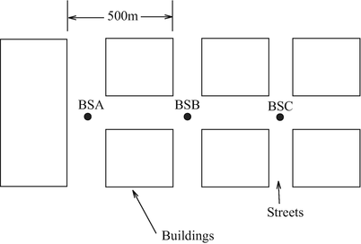

  

  Base station and street layout for Problem 2.56

• The channel bandwidth is 30 kHz

• The propagation environment is characterized by an rms delay spread of σ _τ  = 1 ns

A mobile station is moving from base station A (BSA) to base station B (BSB). Base station C (BSC) is a co-channel base station with BSA.

Explain how you would construct a computer simulator to model the received signal power at the mobile station from (BSA) and (BSC), as the mobile station moves from BSA to BSB. Clearly state your assumptions and explain the relationship between the propagation characteristics in your model.

References

3GPP, Study on 3D channel model for LTE (2015)
A. Abdi, J.A. Barger, M. Kaveh, A parametric model for the distribution of the angle of arrival and the associated correlation function and power spectrum at the mobile station. IEEE Trans. Veh. Technol. 51, 425–434 (2002)
G. Acosta, K. Tokuda, M.A. Ingram, Measured joint Doppler-delay power profiles for vehicle-to-vehicle communications at 2.4 GHz, in IEEE Global Communications Conference, Dallas, TX, November 2004, pp. 3813–3817
A.S. Akki, Statistical properties of mobile-to-mobile land communication channels. IEEE Trans. Veh. Technol. 43, 826–831 (1994)
A.S. Akki, F. Haber, A statistical model of mobile-to-mobile land communication channel. IEEE Trans. Veh. Technol. 35, 2–7 (1986)
J.B. Andersen, T. Rappaport, S. Yoshida, Propagation measurements and models for wireless communications channels. IEEE Commun. Mag. 33, 42–49 (1995)
M.R. Andrews, P.P. Mitra, R. deCarvalho, Tripling the capacity of wireless communications using electromagnetic polarization. Nature 409, 316–318 (2001)
T. Aulin, A modified model for the fading signal at a mobile radio channel. IEEE Trans. Veh. Technol. 28, 182–203 (1979)
P. Bello, Characterization of random time-variant linear channels. IEEE Trans. Commun. 11, 360–393 (1963)
J.-E. Berg, R. Bownds, F. Lotse, Path loss and fading models for microcells at 900 MHz, in IEEE Vehicular Technology Conference, Denver, CO, May 1992, pp. 666–671
G.J. Byers, F. Takawira, Spatially and temporally correlated MIMO channels: modeling and capacity analysis. IEEE Trans. Veh. Technol. 53, 634–643 (2004)
U. Charash, Reception through Nakagami fading multipath channels with random delays. IEEE Trans. Commun. 27, 657–670 (1979)
D.K. Cheng, Field and Wave Electromagnetics, 2nd edn. (Addison-Wesley, Reading, 1989)
S. Chia, R. Steele, E. Green, A. Baran, Propagation and bit-error ratio measurements for a microcellular system. J. Inst. Electron. Radio Eng. (UK) 57, 255–266 (1987)
R. Clarke, A statistical theory of mobile radio reception. Bell System Tech. J. 47, 957–1000 (1968)
COST 207 Digital Land Mobile Radio Communications (Commission of the European Communities, Brussels, 1989)
M. Failli, COST 207 Management Committee, TD(86)51-REV 3 (WG1), Proposal on channel transfer functions to be used in GSM tests late 1986 (1986)
COST 231 TD(91)109, 1800 MHz mobile net planning based on 900 MHz measurements (1991)
COST 231 TD(973)119-REV 2 (WG2), Urban transmission loss models for mobile radio in the 900- and 1,800-MHz bands (1991)
W.B. Davenport, W.L. Root, An Introduction to the Theory of Random Signals and Noise (McGraw-Hill, New York, 1987)
G.W. Davidson, D.D. Falconer, A.U.H. Sheikh, An investigation of block adaptive decision feedback equalization for frequency selective fading channels, in IEEE International Conference on Communications, Philadelphia, PA, June 1988, pp. 360–365
P. Dent, G.E. Bottomley, T. Croft, Jakes fading model revisited. Electron. Lett. 7, 1162–1163 (1993)
E. Eleftheriou, D.D. Falconer, Adaptive equalization techniques for HF channels. IEEE J. Sel. Areas Commun. 5, 238–247 (1987)
V. Erceg, P. Soma, D. Baum, S. Catreux, Multiple-input multiple-output fixed wireless radio channel measurements and modeling using dual-polarized antennas at 2.5 GHz. IEEE Trans. Wirel. Commun. 3, 2288–2298 (2004)
V. Erceg, H. Sampath, S. Catreux-Erceg, Dual-polarization versus single-polarization MIMO channel measurement results and modeling. IEEE Trans Wireless Commun. 5, 28–33 (2006)
ETSI TR 125 943, Univeral Mobile Telecommunications System (UMTS), Deployment aspects 3GPP TR 25.943 version 7.0.0 Release 7 (2007)
R.C. French, Error rate predictions and measurements in the mobile radio data channel. IEEE Trans. Veh. Technol. 27, 214–220 (1978)
R.C. French, The effect of fading and shadowing on channel reuse in mobile radio. IEEE Trans. Veh. Technol. 28, 171–181 (1979)
A.A. Giordano, F.M. Hsu (eds.), Least Square Estimation with Applications to Digital Signal Processing (Wiley, New York, 1985)
A.J. Goldsmith, L.J. Greenstein, A Measurement-based model for predicting coverage areas of urban microcells. IEEE J. Sel. Areas Commun. 11, 1013–1023 (1993)
A.J. Goldsmith, L.J. Greenstein, G.J. Foschini, Error statistics of real time power measurements in cellular channels with multipath and shadowing, in IEEE Vehicular Technology Conference, Secaucus, NJ (1993), pp. 108–110
I. Gradshteyn, I. Ryzhik, Tables of Integrals, Series, and Products (Academic Press, San Diego, 1980)
O. Grimlund, B. Gudmundson, Handoff strategies in microcellular systems, in IEEE Vehicular Technology Conference, Saint Louis, MO, May 1991, pp. 505–510
M. Gudmundson, Analysis of handover algorithms, in IEEE Vehicular Technology Conference, Saint Louis, MO, May 1991, pp. 537–541
M. Gudmundson, Analysis of handover algorithms in cellular radio systems. Report No. TRITA-TTT-9107, Royal Institute of Technology, Stockholm, Sweden, April 1991
M. Gudmundson, Correlation model for shadow fading in mobile radio systems. Electron. Lett. 27, 2145–2146 (1991)
K. Haneda, J. Zhang, L. Tian, G. Liu, Y. Zheng, H. Asplund, J. Li, Y. Wang, D. Steer, C. Li, T. Balercia, S. Lee, Y. Kim, A. Ghosh, T. Thomas, T. Nakamura, Y. Kakishima, T. Imai, H. Papadopoulas, T.S. Rappaport, G.R. MacCartney Jr., M.K. Samimi, S. Sun, O. Koymen, S. Hur, J. Park, C. Zhang, E. Mellios, A.F. Molisch, S.S. Ghassemzadeh, A. Ghosh, 5G 3GPP-like channel models for outdoor urban microcellular and macrocellular environments, in IEEE Vehicular Technology Conference, Nanjing, China, May 2016
P. Harley, Short distance attenuation measurements at 900 MHz and 1. 8 GHz using low antenna heights for microcells. IEEE J. Sel. Areas Commun. 7, 5–11 (1989)
M. Hata, T. Nagatsu, Mobile location using signal strength measurements in cellular systems. IEEE Trans. Veh. Technol. 29, 245–251 (1980)
M.-J. Ho, G.L. Stüber, Co-channel interference of microcellular systems on shadowed Nakagami fading channels, in IEEE Vehicular Technology Conference, Secaucus, NJ, May 1993, pp. 568–571
P. Hoeher, A statistical discrete-time model for the WSSUS multipath channel. IEEE Trans. Veh. Technol. 41, 461–468 (1992)
K. Imamura, A. Murase, Mobile communication control using multi-transmitter simul/sequential casting (MSSC), in IEEE Vehicular Technology Conference, Dallas, TX, May 1986, pp. 334–341
W.C. Jakes, Microwave Mobile Communication (IEEE Press, New York, 1993)
M. Kaji, A. Akeyama, UHF-band propagation characteristics for land mobile radio, in International Symposium on Antennas and Propagation, University of British Columbia, Canada, June 1985, pp. 835–838
C. Komninakis, A fast and accurate Rayleigh fading simulator, in IEEE Communications Conference, San Francisco, CA, December 2003, pp. 3306–3310
I.Z. Kovacs, P.C.F. Eggers, K. Olesen, L.G. Petersen, Investigations of outdoor-to-indoor mobile-to-mobile radio communication channels, in IEEE Vehicular Technology Conference, Vancouver, Canada (2002), pp. 430–434
S. Kozono, T. Suruhara, M. Sakamoto, Base station polarization diversity reception for mobile radio. IEEE Trans. Veh. Technol. 33, 301–306 (1984)
A. Kuchar, J.P. Rossi, E. Bonek, Directional macro-cell channel characterization from urban measurements. IEEE Trans. Antennas Propag. 48, 137–146 (2000)
J. Kunisch, J. Pamp, Wideband Car-to-Car Radio Channel Measurements and Model at 5.9 GHz, in IEEE Vehicular Technology Conference, Calgary, Canada (2008)
S.-C. Kwon, G.L. Stüber, Polarized channel model for body area networks using reflection coefficients
M. Landmann, K. Sivasondhivat, J.-I. Takada, I. Ida, R. Thoma, Polarisation behaviour of discrete multipath and diffuse scattering in urban environments at 4.5 GHz. EURASIP J. Wirel. Commun. Netw., 2007, 60 (2007), Article ID 57980
B. Larsson, B. Gudmundson, K. Raith, Receiver performance for the North American digital cellular system, in IEEE Vehicular Technology Conference, Saint Louis, MO, May 1991, pp. 1–6
W.C.Y. Lee, Mobile Communications Engineering (McGraw Hill, New York, 1982)
W.C.Y. Lee, Mobile Communications Design Fundamentals (SAMS, Indianapolis, 1986)
W. Lee, Y. Yeh, Polarization diversity system for mobile radio. IEEE Trans. Commun. 20, 912–923 (1972)
W.C.Y. Lee, Y.S. Yeh, On the estimation of the second-order statistics of log-normal fading in mobile radio environment. IEEE Trans. Commun. 22, 809–873 (1974)
Y.X. Li, X. Huang, The simulation of independent Rayleigh faders. IEEE Trans. Commun. 50, 1503–1514 (2002)
F. Ling, J.G. Proakis, Adaptive lattice decision-feedback equalizers – their performance and application to time-variant multipath channels. IEEE Trans. Commun. 33, 348–356 (1985)
J.-P.M. Linnartz, Exact analysis of the outage probability in multiple-user mobile radio. IEEE Trans. Commun. 40, 20–23 (1992)
J.M.G. Linnartz, R.F. Fiesta, Evaluation of radio links and networks. California PATH Program (1996) [Online]. Available: http://www.path.berkeley.edu/PATH/Publications/PDF/PRR/96/PRR-96-16.pdf
F. Lotse, A. Wejke, Propagation measurements for microcells in central Stockholm, in IEEE Vehicular Technology Conference, Orlando, FL (1990), pp. 539–541
M.B. Madayam, P.-C. Chen, J.M. Hotzman, Minimum duration outage for cellular systems: a level crossing analysis, in IEEE Vehicular Technology Conference, Atlanta, GA, June 1996, pp. 879–883
M. Marsan, G. Hess, Shadow variability in an urban land mobile radio environment. Electron. Lett. 26, 646–648 (1990)
I. Mathworks, Filter design toolbox for use with MATLAB, User’s Guide (2005)
J. Maurer, T. Fügen, W. Wiesbeck, Narrow-band measurement and analysis of the inter-vehicle transmission channel at 5.2 GHz, in IEEE Vehicular Technology Conference, Birmingham, AL, pp. 1274–1278, 2002.
L.B. Milstein, D.L. Schilling, R.L. Pickholtz, V. Erceg, M. Kullback, E.G. Kanterakis, D. Fishman, W.H. Biederman, D.C. Salerno, On the feasibility of a CDMA overlay for personal communications networks. IEEE J. Sel. Areas Commun. 10, 655–668 (1992)
S. Mockford, A.M.D. Turkmani, Penetration loss into buildings at 900 MHz, in IEE Colloquium on Propagation Factors and Interference Modeling for Mobile Radio Systems, London, UK, pp. 1/1–1/4 (1988)
S. Mockford, A.M.D. Turkmani, J.D. Parsons, Local mean signal variability in rural areas at 900 MHz, in IEEE Vehicular Technology Conference, Orlando, FL, May 1990, pp. 610–615
P.E. Mogensen, P. Eggers, C. Jensen, J.B. Andersen, Urban area radio propagation measurements at 955 and 1845 MHz for small and micro cells, in IEEE Global Communications Conference, Phoenix, AZ, December 1991, pp. 1297–1302
R. Muammar, S.C. Gupta, Cochannel interference in high-capacity mobile radio systems. IEEE Trans. Commun. 30, 1973–1978 (1982)
A. Murase, I.C. Symington, E. Green, Handover criterion for macro and microcellular systems, in IEEE Vehicular Technology Conference, Saint Louis, MO, May 1991, pp. 524–530
M. Nakagami, The m distribution; a general formula of intensity distribution of rapid fading, in Statistical Methods in Radio Wave Propagation, ed. by W.G. Hoffman (Pergamon Press, New York, 1960), pp. 3–36
C. Oestges, V. Erceg, A.J. Paulraj, Propagation modeling of MIMO multipolarized fixed wireless channels. IEEE Trans. Veh. Technol. 53, 644–654 (2004)
Y. Okumura, E. Ohmuri, T. Kawano, K. Fukuda, Field strength and its variability in VHF and UHF land mobile radio service. Rev. ECL 16, 825–873 (1968)
J.D. Parsons, The Mobile Radio Propagation Channel (Wiley, New York, 1992)
J.D. Parsons, A.M.D. Turkmani, Characterisation of mobile radio signals: model description, in IEE Proceedings I, Communications, Speech and Vision, vol. 138 (1991), pp. 549–556
C.S. Patel, G.L. Stüber, T.G. Pratt, Comparative analysis of statistical models for the simulation of Rayleigh faded cellular channels. IEEE Trans. Commun. 53, 1017–1026 (2005)
M. Pätzold, Mobile Fading Channels (Wiley, West Sussex, 2002)
M. Pätzold, U. Killat, F. Laue, Y. Li, On the statistical properties of deterministic simulation models for mobile fading channels. IEEE Trans. Veh. Technol. 47, 254–269 (1998)
M.F. Pop, N.C. Beaulieu, Limitations of sum-of-sinusoids fading channel simulators. IEEE Trans. Commun. 49, 699–708 (2001)
R. Prasad, A. Kegel, Spectrum efficiency of microcellular systems. Electron. Lett. 27, 423–425 (1991)
J.G. Proakis, M. Salehi, Digital Communications, 5th edn. (McGraw-Hill, New York, 2007)
R.I.-R. M.1225, Guidelines for evaluation of radio transmission techniques for IMT-2000 (1997)
T. Rappaport, L. Milstein, Effects of path loss and fringe user distribution on CDMA cellular frequency reuse efficiency, in IEEE Global Communications Conference, San Diego, CA, December 1990, pp. 500–506
S. Rice, Statistical properties of a sine wave plus noise. Bell Syst. Tech. J. 27, 109–157 (1948)
A. Rustako, N. Amitay, G. Owens, R. Roman, Radio propagation at microwave frequencies for line-of-sight microcellular mobile and personal communications. IEEE Trans. Veh. Technol. 40, 203–210 (1991)
M. Shafi, M. Zhang, A. Moustakas, P. Smith, A. Molisch, F. Tufvesson, S. Simon, Polarized MIMO channels in 3-D: models, measurements, and mutual information. IEEE J. Sel. Areas Commun. 24, 514–527 (2006)
W.H. Sheen, G.L. Stüber, MLSE equalization and decoding for multipath-fading channels. IEEE Trans. Commun. 39, 1455–1464 (1991)
P. Soma, D.S. Baum, V. Erceg, R. Krishnamoorthy, A.J. Paulraj, Analysis and modeling of MIMO radio channel based on outdoor measurements conducted at 2.5 GHz for fixed BWA applications, in IEEE International Conference on Communications, April 2002, pp. 272–276
K. Steiglitz, Computer-aided design of recursive digital filters. IEEE Trans. Audio Electroacoust. 18, 123–129 (1970)
R.J. Tront, J.K. Cavers, M.R. Ito, Performance of Kalman decision-feedback equalization in HF radio modems, in IEEE International Conference on Communications, Toronto, Canada, June 1986, pp. 1617–1621
A.M.D. Turkmani, Probability of error for M-branch selection diversity. IEE Proc. I. 139, 71–78 (1992)
A.M.D. Turkmani, J.D. Parsons, F. Ju, D.G. Lewis, Microcellular radio measurements at 900,1500, and 1800 MHz, in 5th International Conference on Mobile Radio and Personal Communications, Coventry, UK, December 1989, pp. 65–68
F. Vatalaro, A. Forcella, Doppler spectrum in mobile-to-mobile communications in the presence of three-dimensional multipath scattering. IEEE Trans. Veh. Technol. 46, 213–219 (1997)
R.G. Vaughan, Polarization diversity in mobile communications. IEEE Trans. Veh. Technol. 39, 177–185 (1990)
J.-F. Wagen, Signal strength measurements at 881 MHz for urban microcells in downtown Tampa, in IEEE Global Communications Conference, Phoenix, AZ, December 1991, pp. 1313–1317
E.H. Walker, Penetration of radio signals into buildings in cellular radio environments. Bell Syst. Tech. J. 62, 2719–2734 (1983)
R. Wang, D. Cox, Channel modeling for ad hoc mobile wireless networks, in IEEE Vehicular Technology Conference, Birmingham, AL (2002), pp. 21–25
A. Williamson, B. Egan, J. Chester, Mobile radio propagation in Auckland at 851 MHz. Electron. Lett. 20, 517–518 (1984)
H. Xia, H. Bertoni, L. Maciel, A. Landsay-Stewart, Radio propagation measurements and modeling for line-of-sight microcellular systems, in IEEE Vehicular Technology Conference, Denver, CO, May 1992, pp. 349–354
C. Xiao, Y.R. Zheng, A statistical simulation model for mobile radio fading channels, in Wireless Communications and Networking Conference, New Orleans, LA, March 2003, pp. 144–149
C. Xiao, Y.R. Zheng, N. Beaulieu, Statistical simulation models for Rayleigh and Rician fading, in IEEE International Conference on Communications, Anchorage, AK, May 2003, pp. 3524–3529
Y. Yamada, Y. Ebine, N. Nakajima, Base station/vehicular antenna design techniques employed in high capacity land mobile communications system. Rev. Electr. Commun. Lab. NTT 35, 115–121 (1987)
D.J. Young, N.C. Beaulieu, The generation of correlated Rayleigh random variates by inverse discrete Fourier transform. IEEE Trans. Commun. 48, 1114–1127 (2000)
A.G. Zajić, G.L. Stüber, A new simulation model for mobile-to-mobile Rayleigh fading channels, in Wireless Communications and Networking Conference, Las Vegas, NV, April 2006, pp. 1266–1270
A.G. Zajić, G.L. Stüber, Efficient simulation of Rayleigh fading with enhanced de-correlation properties. IEEE Trans. Wirel. Commun. 5, 1866–1875 (2006)
Y.R. Zheng, C. Xiao, Improved models for the generation of multiple uncorrelated Rayleigh fading waveforms. IEEE Commun. Lett. 6, 256–258 (2002)
Y.R. Zheng, C. Xiao, Simulation models with correct statistical properties for Rayleigh fading channels. IEEE Trans. Commun. 51, 920–928 (2003)
Author information
Authors and Affiliations