Photons

Abstract

The photon is an elementary particle characterized by its frequency and polarization. The photon displays both wave-like and particle-like behavior. A photon is the unit intensity of the electro-magnetic field. Once created, a photon is characterized by its energy $(E = hf)$ which remains unchanged until the photon is destroyed. Maxwell’s equations describe the electromagnetic fields in the classical regime, including propagation of photon beams as a function of frequency and polarization. Maxwell’s equations represent a staggering accomplishment in physical theory, but they do not give a complete description of photon behavior. Two photons with the same quantum numbers (that is the same frequency and polarization) can (unlike electrons) occupy the same place at the same time. The probability that an energy state is occupied by a photon is given by the Bose-Einstein distribution. A single photon is an indivisible elementary particle. Single photons can be produced by spontaneous parametric down-conversion. This is an optical process that cannot by described using Maxwell’s equations. When a single photon is incident upon a beamsplitter, its wavefunction is separated spatially into two parts, corresponding to reflection and transmission. When a measurement is made, the entire photon will be detected either as 100% transmitted or 100% reflected. This result is an example of the Copenhagen interpretation of quantum mechanics.

Exercises

• 2.1 Using MATLAB , calculate the transmission coefficient of a photon beam through a plate of glass (SiO₂) using the parameters and following the procedure given in Example 2.1. Plot the dependence of the transmission coefficient as a function of wavelength and as a function of frequency. Identify the wavelength above which oscillations in the transmission coefficient no longer occur.

• 2.2 Using Maxwell’s equations, derive the expression for the transmission coefficient and the reflection coefficient for an electromagnetic wave passing from one dielectric material to another with the electric field polarized parallel to the plane of incidence. These expressions are Fresnel’s 3rd and 4th equations.

• 2.3 Derive the analytical expression for photon propagation through a plasma layer when the wavevector is an imaginary number ($k_{2} = i\kappa_{2}$ where $\kappa_{2}$ is real).

Show that:

$$ T \equiv \left\| {\frac{F}{A}} \right\|^{2} = \frac{1}{{\cosh^{2} \left( {\kappa_{2} a} \right) + \frac{1}{4}\left( {\frac{{k_{1}^{2} - \kappa_{2}^{2}}}{{k_{1}^{{}} \kappa_{2}^{{}}}}} \right)^{2} \sinh^{2} \left( {\kappa_{2} a} \right)}} $$

• 2.4 A general interface between two planar regions having indices of refraction $n_{1}$ and $n_{2}$ is shown in Fig. 2.17:

  Fig. 2.17

  

  Diagram of index of refraction versus distance for Exercise 2.4

Show that the general expression for the transfer matrix that summarizes the boundary conditions at the interface at z = Z is:

$$ \left[ {\begin{array}{*{20}c} {} \\ {M_{ij}} \\ {} \\ \end{array}} \right] = \frac{1}{2}\left[ {\begin{array}{*{20}c} \begin{aligned} \left( {1 + R} \right)e^{iZB} \hfill \\ \hfill \\ \end{aligned} & \begin{aligned} \left( {1 - R} \right)e^{ - iZA} \hfill \\ \hfill \\ \end{aligned} \\ {\left( {1 - R} \right)e^{iZA}} & {\left( {1 + R} \right)e^{ - iZB}} \\ \end{array}} \right] $$

where

$$ \begin{aligned} R & = \frac{{k_{2}}}{{k_{1}}} \\ A & = k_{1} + k_{2} \\ B & = k_{2} - k_{1} \\ \end{aligned} $$

k ₁ is the wavevector on the left-hand side and k ₂ is the wavevector on the right side of the interface, and Z is the coordinate of the interface.

• 2.5 Compute the transmission coefficient for photons passing through a grating formed by 5 planar layers of alternating index of refraction, making use of the expression in Exercise 2.4 for the transfer matrix (Fig. 2.18).

  Fig. 2.18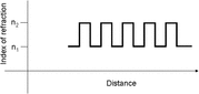

  

  Model structure for a five-layer planar dielectric stack

Evaluate your computing routine using:

$\begin{aligned} n_{1} & = 1.5 \\ n_{2} & = 1.9 \\ \end{aligned}$

Thickness of each region = 500 nm

Over a frequency range: $10^{14}\;\text{Hz} < \omega < 10^{15}\; \text{Hz}$.

Make a plot of the transmission and reflection coefficients as a function of free-space wavelength.

Hint: write a subroutine that determines the transfer matrix for two adjacent interfaces of the structure.

• 2.6 Calculate the transmission coefficient as a function of free-space wavelength for photons passing through a dielectric stack of 11 planar layers of alternating index of refraction, making use of the calculation routine developed in Exercise 2.4. Refer to Fig. 2.19.

• (a) Show that the effect of adding additional layers is to create bands of transmission and reflection.

• (b) Demonstrate which parameters of the calculation determine the width of the transmission bands

• (c) What is the maximum value of reflectivity that you can achieve?

  Fig. 2.19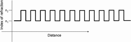

  

  The 11-period structure. The index of refraction is changed periodically, simulating a multi-layer dielectric filter

Evaluate your simulation using

• $n_{1} = 1. 5$, width = 500 nm

• $n_{2} = 3.0$, width = 500 nm

• $500\,{\text{nm}} < \lambda_{free{\text{-}}space} < 1500\,{\text{nm}}$

Such a structure is called a photonic crystal, because it is periodic structure, like a crystal, but with a period that is similar to the wavelength of light that propagates through the structure.

• 2.7 By introducing a defect in the structure of Fig. 2.19 we can change its optical properties. There are different types of defects:

• Vacancy: a layer can be left out of the stack

• Impurity: a layer can have a different index of refraction

• Phase: a layer can be placed at a non-periodic location

Each of these defects can be modelled in a straightforward way using the transfer-matrix method. In this example we show the effect of introducing a phase defect. We advance the position of the 6th layer in the stack by 30% of a full period as shown in Fig. 2.20.

Fig. 2.20

Periodic dielectric contrast grating. The sixth period has been replaced by a phase defect

Referring to Fig. 2.18, introduce a defect in the 11 period structure by enlarging the lower index layer in the center of the periodic structure.

Using the same parameters as those for Exercise 2.5, substitute a $\frac{\lambda}{4}$ phase defect for the 6th period. In a simple form, this could be a section 250 nm in length with $n = n_{1}$

• (a) Calculate the transmission coefficient as a function of free-space wavelength and compare to your result in Exercise 2.4

• (b) Show that the presence of a wider layer introduces a region where transmission can occur in the middle of a region where transmission is normally forbidden. (This is called a defect mode, and is used to achieve single-mode operation of lasers that use photonic crystal reflectors as mirrors.) (see Fig. 2.21 for an example simulation)

• 2.8 Some data taken from the experiment “Existence Photon” on the Quantum Lab website and described in Fig. 2.14 are summarized in Table 2.1. Detector D1 refers to the transmitted photon and detector D2 refers to the reflected photon. T refers to the trigger which heralds the arrival of a single photon at the beam splitter. These data are taken for a series of laser power used to generate photon pairs by spontaneous parametric down conversion (Fig. 2.21)

  Table 2.1 Data for the passage of a single photon passing through a beam splitter

  Fig. 2.21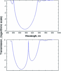

  

  Sample simulation of defect in a dielectric stack. This result shows the effect of a quarter-period phase defect inserted in a dielectric stack. The defect creates a highly transmitting, narrow bandwidth mode in the center of a highly reflecting (R > 0.9999) band

  • (a) Complete the table by calculating the second-order correlation coefficient $g^{2} \left(0 \right)$ for the measurements with trigger and without trigger for laser power = 500 and 50 µW.

  • (b) Comment on the relationship between the determination of $g^{2} \left(0 \right)$ and laser power that you observe in the two cases of trigger and without trigger.

References

H.-A. Bachor, T.C. Ralph, Guide to Experiments in Quantum Optics, 2nd edn. (Wiley-VCH Verlag, Weinheim, 2004). ISBN 13: 978-3-52-740393-6
M. Beck, Quantum Mechanics. Theory and Experiments (Oxford University Press, New York, 2012). ISBN 978-0-19-979812-4
J.S. Bell, Introduction to the hidden variable question, in Proceedings, International School of Physics, ‘Enrico Fermi’, (Academic Press, New York, 1971) pp. 171–81 (Chapter X in Speakable and Unspeakable in Quantum Mechanics, Cambridge University Press, Cambridge, 1987). ISBN 0-521-33495-0
D. Dykstra, S. Busch, W. Peters, M. van Exter, Leiden University CCD (2008). https://www.youtube.com/watch?v=MbLzh1Y9POQ
P. Grangier, G. Roger, A. Aspect, Experimental evidence for a photon anticorrelation effect on a beam splitter: a new light in single photon interferences. Europhys. Lett 1, 173–179 (1986)
E. Hecht, Optics, 2nd edn. (Reading, Addison-Wesley, 1987). ISBN 0-201-11609-X
C. Jönsson, Elektroneninterferenzen an mehreren künstlich hergestellten Feinspalten (Electron interference in a fabricated metal-slit grating). Zeitschrift für Physik 161, 454–474 (1961)
C. Jönsson, Electron diffraction at multiple slits. Am. J. Phys. 42, 4–11 (1974)
C.H. Lineweaver, T.M. Davis, Misconceptions about the Big Bang. Sci. Am., 36–45 (2005)
Quantum Lab, http://www.didaktik.physik.uni-erlangen.de/quantumlab/english/index.htm. An interactive presentation of quantum photon experiments. Project leader: Jan-Peter Meyn, Physikalisches Institut – Didaktik der Physik, Universität Erlangen-Nürnberg
J.J. Thorn, M.S. Neel, V.W. Donato, G.S. Bergreen, R.E. Davies, M. Beck, Observing the quantum behavior of light in an undergraduate laboratory. Am. J. Phys. 72, 1210–1219 (2004). doi:10.1119/1.1737397
A. Tonomura, J. Endo, T. Matsuda, T. Kawasaki, H. Ezawa, Demonstration of single-electron build-up of an interference pattern. Am. J. Phys. 57, 117–120 (1989)
J. Yin, Y. Cao, H.-L. Yong, J.-G. Ren, H. Liang, S.-K. Liao, F. Zhou, C. Liu, Y.-P. Wu, G.-S. Pan, L. Li, N.-L. Liu, Q. Zhang, C.-Z. Peng, J.-W. Pan, Bounding the speed of spooky action at a distance. Phys. Rev. Lett. 110, 260407 (2013). https://arxiv.org/abs/1303.0614
Author information
Authors and Affiliations
Corresponding author