Weighted and Branching Bisimilarities from Generalized Open Maps

Abstract

In the open map approach to bisimilarity, the paths and their runs in a given state-based system are the first-class citizens, and bisimilarity becomes a derived notion. While open maps were successfully used to model bisimilarity in non-deterministic systems, the approach fails to describe quantitative system equivalences such as probabilistic bisimilarity. In the present work, we see that this is indeed impossible and we thus generalize the notion of open maps to also accommodate weighted and probabilistic bisimilarity. Also, extending the notions of strong path and path bisimulations into this new framework, we show that branching bisimilarity can be captured by this extended theory and that it can be viewed as the history preserving restriction of weak bisimilarity.

Supported by the NWO TOP project 612.001.852.

1 Introduction

The theory of open maps is a categorical framework to reason about systems and their bisimilarities [16]. Given a category of systems and a description of the shape of the executions and how to extend them, open maps are morphisms with lifting properties with respect to those extensions. Intuitively, open maps are morphisms which preserve and reflect transitions of systems, that is, they are morphisms whose graphs are bisimulations. The theory covers various classical notions of bisimilarity. For example, two LTSs are strongly bisimilar if and only if there is a span of open maps between them. Varying the category of models and the execution shapes allows describing weak bisimilarity, timed bisimilarity, probabilistic Larsen and Skou bisimilarity, and history-preserving bisimilarity of event structures (see [3, 12, 16] for examples).

Another categorical framework for bisimilarity is coalgebra [22]. This time, given a category and an endofunctor describing respectively the type of state spaces and the type of transitions, a ‘system’ is understood as a coalgebra for this functor. Coalgebra homomorphisms are then very similar to open maps in spirit: they also are morphisms that preserve and reflect transitions. This intuition has been made formal by transformations between the categorical frameworks in both ways; from open maps to coalgebra [19], and conversely [25]. However, the latter suggests that open maps are only adapted to modeling non-deterministic systems and would struggle with other types of branchings, such as probabilistic.

In coalgebra, there are no particular difficulties in modeling weighted systems, and by extension, discrete probabilistic systems [17]. There is also some work for continuous probabilities, although the theory is much more complicated [4, 5]. As we will explain more precisely later, there have been some attempts to do so with open maps in [3, 5], but the result is somewhat disappointing.

Conversely, coalgebra is not adapted to bisimilarities for systems where transitions are not history-preserving, that is, for which the behavioral equivalence does not just depend on the transitions at a given state, but on the whole history of the execution that led to this state. That is the case for example for branching bisimilarity [23]. Branching bisimilarity arose precisely to make weak bisimilarity history-preserving. In [3], weak bisimilarity has been described using open maps by carefully choosing the underlying category, with a general theory developed in [9] using presheaf models. Branching bisimilarity has also been studied using open maps in [1, 2], but indirectly, through a translation into presheaves.

To resume, the goal of this paper is to capture weighted and branching bisimilarities using a generalization of open maps. Concretely, the contributions are:

• 1. a proof that it is impossible to appropriately model probabilistic system using standard open maps (Section 3.2),

• 2. a faithful extension of the theory of open maps and (strong) path bisimulations (Section 4),

• 3. a generalized open map situation capturing weighted and probabilistic bisimilarities (Section 5),

• 4. a generalized open map situation where strong path bisimulations correspond to stuttering branching bisimulations, open map bisimilarity to branching bisimilarity, and path bisimulations to weak bisimulations (Section 6).

Full proofs can be found in the appendix: http://arxiv.org/abs/2301.07004

2 From Path Categories to Bisimilarity

Before discussing weighted bisimilarity, let us first recall the main ideas of modeling bisimilarity via open maps, as introduced by Joyal et al. [16]. The definition is parametric in a functor $J:\mathbb {P}\rightarrow \mathbb {M}$, from a category $\mathbb {P}$ of paths to a category $\mathbb {M}$ of models or systems of interest. In the prime example, $\mathbb {M}$ is the category of labelled transition systems $\textsf{LTS}$ as defined next:

Definition 2.1

For a fixed set A of labels, the category $\textsf{LTS}$ contains:

• 1. Objects: a labelled transition system

  

  is a set X of states, a transition relation

  

  and a distinguished initial state $x_0\in X$. We write

  

  to denote that

  

  and simply refer to the LTS as X if

  

  and $x_0$ are clear from the context. For disambiguation, we use $\rightarrow$ for morphisms and

  

  for transitions.

• 2. Morphisms: a functional simulation

  

  is a function $f:X\rightarrow Y$ with $f(x_0) = y_0$ and for all

  

  in X, we have

  

  .

A functional simulation $f:X\rightarrow Y$ intuitively means that the system Y has at least the transitions of X, but possibly more. A special case of a functional simulation is the run of a word in a system:

Definition 2.2

For the label set A, let $(A^*,\le )$ be the partially ordered set of words, ordered by the prefix ordering. The functor $J:(A^*,\le )\rightarrow \textsf{LTS}$ sends a word $w\in A^*$ to the LTS

of all prefixes of w with

for all $a\in A$, $va\le w$.

This functor J (or more precisely, its image) is often called path category of $\textsf{LTS}$: the possible runs of a word $w\in A^*$ in

correspond precisely to the functional simulations

in $\textsf{LTS}$.

On the abstract level, for a general functor $J:\mathbb {P}\rightarrow \mathbb {M}$, we understand the set of morphisms $r:Jw\rightarrow X$ for $w\in \mathbb {P}$ and $X\in \mathbb {M}$ as the runs of the path w in the model X. We can already make the trivial observation that all morphisms $f:X\rightarrow Y$ in $\mathbb {M}$ preserve runs: given a run $r:Jw\rightarrow X$ of some path $w\in \mathbb {P}$ in X, there is a run $f\cdot r:Jw\rightarrow Y$ of w in Y.

The converse does not hold for a general $f:X\rightarrow Y$ in $\mathbb {M}$: given a run of w in Y, there is not necessarily a run of w in X. If f reflects runs, it is called open:

Definition 2.3

For a functor $J:\mathbb {P}\rightarrow \mathbb {M}$, a morphism $f:X\rightarrow Y$ in $\mathbb {M}$ is called open if f satisfies the following lifting property for all $e:v\rightarrow w$ in $\mathbb {P}$:

That is, for all commutative squares ($s\cdot Je = f\cdot r$), there is $d:Jw\rightarrow X$ in $\mathbb {M}$ that makes both triangles on the right commute ($f\cdot d = s$ and $d\cdot Je= r$).

By construction, we can only make statements about states that are reachable via some run. Thus, one often restricts $\mathbb {M}$ beforehand to contain only models in which all states are reachable from the initial state.

For LTSs in which all states are reachable from the initial state, open maps are related to strong bisimulations [20]: open maps are precisely functions whose graph relation $\{(x,fx) \mid x \in X\}$ is a strong bisimulation. Reformulated in the context of allegories [10], open maps are precisely the maps in the allegory of relations that are strong bisimulations. It is then natural to recover bisimulations as tabulations of open maps, that is:

Definition 2.4

For a functor $J:\mathbb {P}\rightarrow \mathbb {M}$, we say that two models X and Y are J-bisimilar, if there exist another model Z and two J-open maps $f:Z\rightarrow X$ and $g:Z\rightarrow Y$, that is, if there is a span of J-open maps between them.

Of course, J-bisimilarity is a reflexive (identities are open maps) and symmetric (by permuting f and g in the definition) relation on models, but it is not transitive in general. It is when the category $\mathbb {M}$ has pullbacks [16].

Given a functor $J:\mathbb {P}\rightarrow \mathbb {M}$, there are more classical ways of defining bisimilarities given in [16]. The first one is (strong) path bisimulations, which are relations on runs (similar to history-preserving bisimulations) satisfying the usual bisimilarity conditions. The second one is by using a modal logic similar to the Hennessy-Milner theorem. In the case of LTSs with strong bisimilarity, all those notions describe the same notion of bisimilarity, but that is not true for general $J:\mathbb {P}\rightarrow \mathbb {M}$: it can only be proved that J-bisimilarity implies the existence of a (strong) path bisimulation, which itself implies that the two models satisfy the same formulas of the modal logic. In [6], some mild sufficient conditions in terms of trees (i.e., colimits of paths in $\mathbb {M}$) are given for those three notions to coincide. In particular, all the examples of bisimilarities covered by open maps cited earlier satisfy these conditions.

We use coalgebra for uniform statements about state-based systems of different branching type (including non-deterministic and probabilistic branching):

Definition 2.5

For an object 1 of a category $\mathcal {C}$ and an endofunctor $F:\, \mathcal {C}\rightarrow \mathcal {C}$, a pointed coalgebra is a pair of morphisms of $\mathcal {C}$ of the form $1 \xrightarrow {~i~} X \xrightarrow {~\xi ~} FX.$

For example, LTSs can be modeled as pointed coalgebras with $\mathcal {C}= \textsf{Set}$, 1 any singleton, and $F = \mathcal {P}(A\times \_)$, where $\mathcal {P}$ is the power set functor. The usual notion of morphisms of coalgebras can be spelt out as follows:

Definition 2.6

A (proper) homomorphism of pointed coalgebras from $(X,\xi ,i)$ to $(Y,\zeta ,j)$ is a morphism $f:\, X \rightarrow Y$ of $\mathcal {C}$ such that the diagram on the right commutes.

Pointed coalgebras and proper homomorphisms always form a category, but in the case of LTSs as described above, this category is not equivalent to the category $\textsf{LTS}$. Indeed, proper homomorphisms are not just morphisms that preserve transitions, but similarly to open maps, they also reflect them. In [25], the authors proved that for a large class of endofunctors, whose coalgebras basically are non-deterministic, proper homomorphisms precisely correspond to J-open maps for a certain functor J. To model morphisms that are only required to preserve transitions, homomorphisms have to be made lax as follows (see [25]):

Definition 2.7

Assume a relation $\sqsubseteq$ on every Hom-set $\mathcal {C}(X,FY)$. A lax homomorphism of pointed coalgebras from $(X,\xi ,i)$ to $(Y,\zeta ,j)$ is a morphism $f:\, X \rightarrow Y$ of $\mathcal {C}$ such that the diagram on the right laxly commutes, that is, $f\cdot i = j$ and $Ff\cdot \xi \sqsubseteq \zeta \cdot f$ in $\mathcal {C}(X,FY)$.

In the case of the functor $\mathcal {P}(A\times \_)$, we can consider the pointwise inclusion on every Hom-set $\textsf{Set}(X,\mathcal {P}(A\times Y))$. With this, pointed coalgebras and lax homomorphisms form a category which is isomorphic to the category $\textsf{LTS}$. However, it is not true in general that they form a category, as a compatibility of $\sqsubseteq$ with the composition is needed as follows:

Definition 2.8

A partial order on F is a collection of partial orders $\sqsubseteq$, one for each Hom-set of the form $\mathcal {C}(X,FY)$ such that

$$ \forall X\xrightarrow {f_1,f_2} FY,~ X'\xrightarrow {g} X,~ Y\xrightarrow {h} Y':~~ f_1 \sqsubseteq f_2 ~~\Rightarrow ~~ Fh\cdot f_1 \cdot g \sqsubseteq Fh\cdot f_2 \cdot g. $$

This is equivalent to the requirement that the Hom-functor $\mathcal {C}(\_\!\!\!\_, F\_\!\!\!\_)$ factors through partially ordered sets: $\mathcal {C}(\_\!\!\!\_, F\_\!\!\!\_):\mathcal {C}^\textsf{op}\times \mathcal {C}\rightarrow \textsf{Pos}.$

Remark 2.9

The present definition subsumes the definition of order on a Set-functor established by Hughes and Jacobs [11, Def 2.1] (details in the appendix).

Lemma 2.10

([25]). When $\sqsubseteq$ is a partial order on F, pointed coalgebras and lax homomorphisms form a category, which we denote by $\textsf{LCoalg} (1,F)$.

Much as with open maps, many flavors of bisimilarity can be recovered using spans of proper homomorphisms:

Definition 2.11

We say that two pointed coalgebras are coalgebraically bisimilar if there is a span of proper homomorphisms between them.

There are many ways of defining bisimilarities in coalgebra (see [13] for an overview), but they coincide for the purpose of the present paper.

3 Weighted Bisimilarity and Open Maps

In this section, we describe known attempts to model weighted systems, and particularly probabilistic ones, using open maps. They all work with some variations of the (discrete) distribution functor on $\textsf{Set}$. We will denote this functor, which maps a set X to the set

$$ \mathcal {D} X = \big \{ f:X \rightarrow [0,1] \mid f^{-1}\big ((0,1]\big )\text { is finite and } \sum _{x\in X} f(x) = 1\big \}, $$

by $\mathcal {D}$ and the variation where the condition $= 1$ is replaced by $\le 1$ by $\mathcal {D}_{\le 1}$ (i.e. $\mathcal {D}_{\le 1} X := \mathcal {D} (X + 1)$). We will prove that, even though Larsen-Skou bisimulations for reactive systems can be modeled with open maps, that is impossible for bisimulations for generative systems.

3.1 Larsen-Skou Bisimilarity Using Open Maps

In [3], Cheng et al. describe an open map situation for Probabilistic Transition Systems (PTSs), which corresponds to coalgebras for the functor $(\mathcal {D} (\_\!\!\!\_)+1)^A$. In this setting, they consider Partial PTSs (PPTS) which are coalgebras for $(\mathcal {D}_{\le 1} ^\varepsilon (\_\!\!\!\_)+1)^A$ where the sub-probability distributions can have values in hyperreals, allowing infinitesimals $\varepsilon$. The category of PTSs embeds in that of PPTSs, and the path category is the full subcategory of PPTSs consisting of finite linear systems whose probabilities of transitions are infinitesimals. It is then proved that J-bisimilarity, restricted to PTSs, for this path category corresponds to Larsen-Skou’s probabilistic bisimilarity [18].

This open map situation has been reformulated in [7] in terms of coreflections: the obvious functor from PPTSs to TSs is a coreflection whose left-adjoint maps a LTS T to the PPTS whose underlying LTS is T and where all transitions have infinitesimal probabilities. In general, given a coreflection $F:\,\mathcal {C}\,\rightarrow \,\mathcal {D}$ with left-adjoint G and a path category J on $\mathcal {D}$, one automatically has the path category $G\circ J$ on $\mathcal {C}$, and this construction preserves good properties of J. In particular, one has that two systems A and B are $(G\circ J)$-bisimilar if and only if FA and FB are J-bisimilar. Cheng et al.’s path category is obtained in this manner with the coreflection above and the standard path category on LTSs. In particular, it means that two PPTSs are bisimilar if and only if their underlying TSs are strongly bisimilar.

3.2 Impossibility Result for Generative Systems

In [5], Desharnais et al.  describe several bisimilarities for generative probabilistic systems, that is, coalgebras for the functor $\mathcal {D}_{\le 1} (A\times \_\!\!\!\_)$, in a coalgebraic way. They pointed out that their efforts to model those bisimilarities using open maps failed [5, p. 188]. In the following, we see that it is in fact not possible. We will show that for generative probabilistic systems modeled by the category $M:=\textsf{LCoalg} (1,\mathcal {D}_{\le 1} (A\times \_\!\!\!\_))$, there is no open map characterization of the coalgebraic bisimilarity. Actually, the argument here is valid for many other types of weights and is not limited to reals.

Here, for two functions $f,g:X \rightarrow \mathcal {D}_{\le 1} (Y)$, $f \sqsubseteq g$ means that for all $x \in X$, for all $y \in Y$, $f(x)(y) \le g(x)(y)$, where $\le$ is the usual ordering on [0, 1].

In this situation:

Theorem 3.1

For $\mathbb {M}:= \textsf{LCoalg} (1,\mathcal {D}_{\le 1} (A\times \_\!\!\!\_))$ there is no category $\mathbb {P}$ and no functor $J:\mathbb {P}\rightarrow \mathbb {M}$ such that for every $h:X\rightarrow Y$ with reachable X the following equivalence holds:

$$ h\text { is { J}-open} \quad \Longleftrightarrow \quad h\text { is a proper homomorphism} $$

and there is no $\mathbb {P}$ and no functor J such that for every X and Y:

$$ X\text { and }Y\text { are }J\text {-bisimilar} \quad \Longleftrightarrow \quad X\text { and }Y\text { are coalgebraically bisimilar}. $$

Proof

(Sketch). By contradiction, assume that there is such a J. We prove that there is a proper homomorphism of the form:

which cannot be J-open. Consider first the unique lax homomorphism $0_\mathbb {M}\rightarrow Y$ where $0_\mathbb {M}$ consists in one state and no transition. This is not a proper homomorphism, so it is not open by assumption. That is there is a square:

with no lifting. It is mechanical to check that $JP \simeq 0_\mathbb {M}$ and JQ has at least one transition from its initial state to another state

with $w \ne 0$. With $n = 2\cdot \lceil \frac{1}{w}\rceil$, the proper homomorphism h above is not open: there cannot be a morphism from JQ to X because $w > \frac{1}{n}$.    $\square$

4 Generalized Open Maps

The main argument of the proof of impossibility is the fact that sometimes, a transition with some probability w in the codomain comes from probabilities $w_1, \ldots , w_n$ with $\sum _i w_i = w$ in the domain, which makes a lifting morphism impossible with the current framework of open maps.

In this section, we will extend the open map framework with the main intuition that the lifting morphism splits the probability w into smaller parts $w_1,\ldots , w_n$. After defining these generalized open maps, we show some basic properties of the bisimilarity generated by them.

4.1 Generalized Open Maps Situation

Here, we describe our extension of the open maps framework. The data is similar: we start with a category of models $\mathbb {M}$, but we need more than just a functor $J:\mathbb {P}\rightarrow \mathbb {M}$. Assume:

• a set V together with a function $J:V \rightarrow \textrm{ob}(\mathbb {M})$,

• two small categories $\mathbb {E}$ and $\mathbb {S}$ whose sets of objects are V,

• two functors $J_{\mathbb {E}}:\mathbb {E}\rightarrow \mathbb {M}$ and $J_{\mathbb {S}}:\mathbb {S}\rightarrow \mathbb {M}$ coinciding with J on objects.

The classical open maps situation $J:\mathbb {P}\rightarrow \mathbb {M}$ fits in this extension as follows. The category $\mathbb {E}$ is given by $\mathbb {P}$ with the intention that they model path shapes and their extensions. The functor $J_{\mathbb {E}}$ is given by J. The category $\mathbb {S}$ is given by the discrete category $|\mathbb {P}|$, that is, the category whose objects are those of $\mathbb {P}$ and whose morphisms are only identities. The functor $J_{\mathbb {S}}$ is the only possible one respecting the conditions of the definition above.

In the general context of this extension, the interpretation is a bit different. Now V is meant to be a set of trees labelled by alphabets and weights. $\mathbb {E}$ still consists in extensions, extending trees into trees with longer branches. $\mathbb {S}$ then consists in merging morphisms, similar to the description above: for the example of weighted systems, those morphisms are allowed to merge states into one, as long as they sum up the weights of the in-going branches. Generally, those morphisms are allowed to perform some merges that are harmless for bisimilarity.

With this data, we can define generalized open maps:

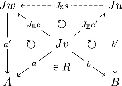
Definition 4.1

A morphism $f:X\rightarrow Y$ in $\mathbb {M}$ is called ( $\mathbb {E}$ , $\mathbb {S}$ )-open if it satisfies the following lifting property for all $e:v\rightarrow w$ in $\mathbb {E}$:

The interpretation starts the same as in usual open maps. Assume that we have a tree y in Y extending the image by f of the tree x in X. If f is open, there should be a tree $x'$ extending x and whose image by f is y. However, $x'$ may have a different shape than y, since it might be necessary to split transitions. That is what u and s are modeling: w is obtained from u by merging some states.

The connection with the classical open maps can be formulated as follows

Proposition 4.2

Given a functor $J:\mathbb {P}\rightarrow \mathbb {M}$ and a morphism $f:X\rightarrow Y$,

$$ f\text { is }J\text {-open if and only if }f\text { is }(\mathbb {P},|\mathbb {P}|)\text {-open.} $$

Again, bisimilarity can be defined as the existence of a span of open maps

Definition 4.3

We say that X and Y are $(\mathbb {E},\mathbb {S})$-bisimilar if there is a span of $(\mathbb {E},\mathbb {S})$-open maps between them.

4.2 Basic Properties

In this section, we will prove general properties of $(\mathbb {E},\mathbb {S})$-bisimilarity similar to the classical case. First, we show that if $\mathbb {M}$ has pullbacks, then $(\mathbb {E},\mathbb {S})$-bisimilarity is an equivalence relation. Secondly, we describe two notions of path bisimulations, both implied by $(\mathbb {E},\mathbb {S})$-bisimilarity. Finally, we prove that it is enough to check openness on some generators of $\mathbb {E}$.

In order to see when $(\mathbb {E},\mathbb {S})$-bisimilarity is an equivalence relation, we need to check symmetry, reflexivity, and transitivity. Symmetry always holds because we can always swap the legs of the span. For reflexivity, it is enough to prove that identities are open which is valid because $\mathbb {S}$ is a category and $J_{\mathbb {S}}$ is a functor, as shown in the diagram on the right. The proof of transitivity relies on composition and pullbacks:

Lemma 4.4

$(\mathbb {E},\mathbb {S})$-open maps are closed under composition and pullbacks.

Theorem 4.5

If $\mathbb {M}$ has pullbacks, then $(\mathbb {E},\mathbb {S})$-bisimilarity is a transitive relation, and thus is an equivalence relation.

Generalized Path Bisimulations. In the classical open map setup [16], another notion of bisimilarity can be defined by using path extensions directly: so-called strong path and path bisimulations, which can be generalized as follows. Like originally [16], we assume that there is an element $0 \in V$, such that J0 is an initial object of $\mathbb {M}$ (note that 0 is not required to be initial in $\mathbb {E}$ or $\mathbb {S}$). The intuition is that the unique morphism $!_X:J0\rightarrow X$ points to the initial state of X. For example, J0 can be given by $(1,\textrm{id} _1,\bot )$ in a category of pointed coalgebras if 1 is the final object of $\mathcal {C}$ and if $\mathcal {C}(1,F1)$ has the least element $\bot :1\rightarrow F1$ (those conditions hold in the cases of interest).

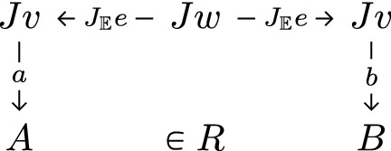
Definition 4.6

A path simulation from A to B in $\mathbb {M}$ is a set R of spans of the form $A \xleftarrow {~a~} Jv \xrightarrow {~b~} B$ (for $v\in V$) satisfying the following two properties

• initial condition: the span $A \xleftarrow {~!_A~} J0 \xrightarrow {~!_B~} B$ belongs to R.

• forward closure: for all spans $A \xleftarrow {~a~} Jv \xrightarrow {~b~} B$ in R, all $e:v\rightarrow w \in \mathbb {E}$ and all $a':Jw\rightarrow A \in \mathbb {M}$ such that $a = a'\cdot J_{\mathbb {E}}e$, there are $e':v\rightarrow u \in \mathbb {E}$, $s:u\rightarrow w \in \mathbb {S}$, and $b':Ju\rightarrow B \in \mathbb {M}$ such that $J_{\mathbb {E}}e = J_{\mathbb {S}}s\cdot J_{\mathbb {E}}e'$, $b = b'\cdot J_{\mathbb {E}}e'$, and the span $A \xleftarrow {~a'\cdot J_{\mathbb {S}}s~} Ju \xrightarrow {~b'~} B$ belongs to R.

  

We say that R is a strong path simulation if it additionally satisfies the following:

• backward closure: for all spans $A \xleftarrow {\,a\,} Jv \xrightarrow {\,b\,} B$ in R and all $e:w\rightarrow v \in \mathbb {E}$, we have that the span $A \xleftarrow {~a\cdot J_{\mathbb {E}}e~} Jw \xrightarrow {~b\cdot J_{\mathbb {E}}e~} B$ belongs to R.

  

We say that R is a (strong) path bisimulation from A to B if R and $R^\dagger = \{B \xleftarrow {~b~} Jv \xrightarrow {~a~} A \mid A \xleftarrow {~a~} Jv \xrightarrow {~b~} B \in R\}$ are (strong) path simulations.

Remark that this version of (strong) path bisimulations has the same type as the one by Joyal et al. [16], but satisfies more general conditions. In particular, when $\mathbb {S}$ is a discrete category, the formulation above is exactly the one from [16]. Obviously, a strong path bisimulation is a path bisimulation.

The main result of this section is the following.

Theorem 4.7

Assume two models A and B in $\mathbb {M}$. If there is a span $A \xleftarrow {~f~} C \xrightarrow {~g~} B$ where g is a morphism of $\mathbb {M}$ and f is an $(\mathbb {E},\mathbb {S})$-open map, then the following set is a strong path simulation:

$$ R_{f,g} := {\{ A \xleftarrow {~a~} Jv \xrightarrow {~b~} B \mid \exists c:Jv\rightarrow C \text { with } a = f\cdot c \text { and } b = g\cdot c \}} $$

Consequently, if A and B are $(\mathbb {E},\mathbb {S})$-bisimilar, then there is strong path bisimulation between them.

As in the classical case of [16], there is no reason for the converse to be true in general: there might be a strong path bisimulation between two models, but no span of generalized open maps. However, conditions from [6] could be accommodated to describe a general framework in which the converse holds. Since this is not the main focus of this paper, we will not do it here, but will show a particular case in Section 6.

Generators of the Category of Extensions. In the first example of open maps for LTSs introduced in Section 2, the path category was described as the poset of words with the prefix order. Consequently, to prove that a functional simulation is J-open, we have to prove the lifting property of Definition 4.1 with respect to all pairs $w \le w'$. However, it is sufficient to check the lifting property for extensions by one letter: $w' = w.a$ for some $a \in A$. The general reason is that, as a category, $(A^*,\le )$ is generated by the morphisms $w \le w.a$, and verifying the lifting property with respect to generators of the category $\mathbb {P}$ is enough to obtain J-openness. This can be extended to generalized open maps, with additional care.

Proposition 4.8

Assume a subgraph $\mathbb {E}'$ of $\mathbb {E}$ that generates $\mathbb {E}$, that is, every morphism of $\mathbb {E}$ is a finite composition of morphisms of $\mathbb {E}'$. Assume additionally, that for every $e \in \mathbb {E}'$ and $s \in \mathbb {S}$ for which $J_{\mathbb {E}}e \cdot J_{\mathbb {S}}s$ is well-defined, there are $s' \in \mathbb {S}$ and $e' \in \mathbb {E}'$ such that $J_{\mathbb {E}}e \cdot J_{\mathbb {S}}s = J_{\mathbb {S}}s' \cdot J_{\mathbb {E}}e'$.

In that case, if a morphism of $\mathbb {M}$ satisfies the lifting property of Definition 4.1 for all morphisms in $\mathbb {E}'$, then it is $(\mathbb {E},\mathbb {S})$-open. Also, if a set of spans satisfies the conditions of Definition 4.6, where $\mathbb {E}$ is replaced by $\mathbb {E}'$, then it is a (strong) path bisimulation.

The first condition is satisfied when $\mathbb {E}$ is a free category and $\mathbb {E}'$ is its class of generators. The second condition is satisfied for e.g. $\mathbb {E}= \mathbb {P}$ and $\mathbb {S}= |\mathbb {P}|$.

5 Open Maps for Weighted Systems

In this section, we will prove that weighted systems can be captured by this generalized open map theory for a large variety of weights, including those needed to capture probabilistic systems.

5.1 Category of Coalgebras for Weighted Systems

In this section, we will consider weighted functors as follows.

Definition 5.1

Given a commutative monoid $(K, +, e)$, the K-weighted functor ${(K,+,e)}^{(\_)}:\textsf{Set}\rightarrow \textsf{Set}$ is defined as follows on sets and maps:

$$\begin{aligned}&\,\,\, \text {sets:} \qquad \qquad \,\, X ~~\mapsto ~~ {(K,+,e)}^{(X)}= {\big \{\mu :X\rightarrow K \mid \mu ^{-1}(K\setminus \{e\}) \text { is finite}\big \}}\\&\text {maps:} \quad f:X\rightarrow Y ~\mapsto ~ {(K,+,e)}^{(f)}(\mu ) = \big (y \in Y \mapsto \sum {\{\mu (x) \mid x\in X, f(x) = y\}} \big ) \end{aligned}$$

An element $\mu$ of $(K,+,e)^{(X)}$ is a finite distributions sending each $x\in X$ to a weight in K. Whenever a map $f:X\rightarrow Y$ identifies elements $f(x_1) = f(x_2) = \cdots$, then the functor action turns $\mu$ into a distribution on Y by adding up the weights $\mu (x_1) + \mu (x_2) + \cdots$ as elements of X are sent to the same element in Y. Since $\mu$ is finite and K is commutative, this addition is well-defined.

Given a commutative monoid $(K, +, e)$ and an alphabet A, we want to consider weighted systems as coalgebras for the functor ${(K,+,e)}^{(A\times \_)}$. As described in Section 2, we want to be able to talk about lax homomorphisms, so we need an order on ${(K,+,e)}^{(A\times \_)}$ as in Definition 2.8. For that, we need to assume an ordered commutative monoid $(K,+,e,\sqsubseteq )$, that is, a monoid $(K, +, e)$ with a partial order $\sqsubseteq$ such that $+$ is monotone in both its arguments.

Lemma 5.2

Given an ordered commutative monoid $(K,+,e,\sqsubseteq )$, then for all sets X and Y, the relation on the hom-set $\textsf{Set}\big (X,{(K,+,e)}^{(A\times Y)}\big )$ defined by

$$ f_1 \sqsubseteq f_2 ~\Longleftrightarrow ~ \forall x\in X,\, \forall y\in Y,\, \forall a \in A,\, f_1(x)(a,y) \sqsubseteq f_2(x)(a,y) $$

is an order on ${(K,+,e)}^{(A\times \_)}$.

So, we have a category $\textsf{LCoalg} \left( 1,{(K,+,e)}^{(A\times \_)}\right)$ of pointed coalgebras and lax homomorphisms. The goal of this section is to design a generalized open maps situation for which $(\mathbb {E},\mathbb {S})$-bisimilarity characterizes coalgebraic bisimilarity and more precisely for which $(\mathbb {E},\mathbb {S})$-openness characterizes proper homomorphisms.

In the course of the constructions and proofs, we will need additional assumptions that we list here.

Definition 5.3

We call an ordered commutative monoid $(K,+,e,\sqsubseteq )$ a rearrangement monoid if it satisfies the additional requirement that if $n,m\ge 1$ and

$$ \sum \limits _{i=1}^n x_i \sqsubseteq \sum \limits _{j=1}^m y_j, $$

then there exists a family $(u_{i,j})_{1\le i \le n,1\le j\le m}$ such that

$$ \text {for all } j,\, \sum \limits _{i=1}^n u_{i,j} \sqsubseteq y_j ~~\text {and}~~ \text {for all } i,\, \sum \limits _{j=1}^m u_{i,j} = x_i. $$

In addition, we say that a rearrangement monoid is strict if the condition above holds also when replacing $\sqsubseteq$ with $=$.

The intuition is as follows. We have some weights arranged as $x_1, \ldots , x_n$. We want to be able to decompose those weights into smaller weights, the $u_{i,j}$s, and by rearranging those small weights obtaining weights smaller than the $y_j$. This condition states that this is possible when there is enough weight in total. The special case of strictness is called the row-column property in [17].

Lemma 5.4

For any subgroup G of the real numbers $(\mathbb {R}^n,+,-,0)$ such that for all x, y in G $(\min (x_1,y_1), \ldots , \min (x_n,y_n)) \in G$, the monoids $(G,+,0,\le )$ and $(G_{\ge 0},+,0,\le )$, where $\le$ is the usual order on $\mathbb {R}^n$, are strict rearrangement monoids.

For any lattice with bottom element $(L, \le , \sqcup , \sqcap , \bot )$, $(L,\sqcup , \bot , \le )$ is a rearrangement monoid if and only if $(L, \le , \sqcup , \sqcap )$ is distributive. Furthermore, in that case, it is always strict.

Another property is a form of positivity: we say that an ordered monoid is positively ordered if e is the bottom element for $\sqsubseteq$, that is, for all $k \in K$, $e \sqsubseteq k$.

Example 5.5

The positive real line $(\mathbb {R}_+,+,0,\le )$ is a positively ordered strict rearrangement monoid and it is necessary to define probabilistic systems. Another example is the monoid of natural numbers $(\mathbb {N},+,0,\le )$, which defines the bag functor. Finally, any distributive lattice with bottom element $(L,\sqcup ,\bot ,\le )$, typically powerset lattices $(\mathcal {P}(X),\cup ,\varnothing ,\subseteq )$, is too. On the contrary, $(\mathbb {R},+,0,\le )$ and $(\mathbb {Z},+,0,\le )$ are strict rearrangement monoids but are not positively ordered. Conversely $(\mathbb {N}_{\ge 1},\times ,1,\le )$ is positively ordered but not a rearrangement monoid. Indeed, it is impossible to rearrange the inequality $2\times 5 \le 3\times 4$.

5.2 Generalized Open Maps Situation for Weighted Systems

Let $(K,+,e,\sqsubseteq )$ be a commutative ordered monoid. Elements of $V_K$ are

• either words on $A\times (K\setminus \{e\})$, $w = (a_1,k_1), \ldots , (a_n,k_n)$,

• or triples $(w_1,b,w_2)$ of a word $w_1$ on $A\times (K\setminus \{e\})$, a letter $b \in A$, and a non-empty word $w_2$ on $(K\setminus \{e\})$.

The function $J_K$ maps

• a word $w = (a_1,k_1), \ldots , (a_n,k_n)$ to the system

  

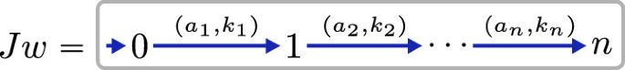
  that is, to the coalgebra $Jw:\{0, \ldots , n\}\rightarrow {K}^{(A\times \{0,\ldots ,n\})}$ such that if $b = a_{i+1}$ and $j = i+1$ then $Jw(i)(b,j) = k_{i+1}$, else $= e$.

• a triple $(w_1,b,w_2)$ with $w_1 = (a_1,k_1), \ldots , (a_n,k_n)$ and $w_2 = l_1, \ldots , l_m$ is mapped to the system

  

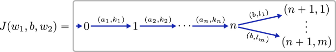
  that is, $J(w_1,b,w_2)(n)(n+1,i) = (b,l_i)$.

Fig. 1.

Example of a lifting of a path extension in $\mathbb {R}_+$-weighted systems and for a singleton label alphabet $|A|=1$, thus omitting action labels.

The category $\mathbb {E}_K$ is defined as follows. For every $w_1$, b, and $w_2$, there is a unique edge e from $w_1$ to $(w_1, b, w_2)$. The functor then maps this edge e to $J_{\mathbb {E}}e$, the obvious injection.

The category $\mathbb {S}_K$ has two types of morphisms:

• identities on words $w_1$,

• morphisms from $(w_1, b, w_2')$ to $(w_1, b, w_2)$, with $w_2' = l_1',\ldots ,l_{m'}'$ and $m \le m'$, which are given by surjective monotone functions $s:\{1,\ldots ,m'\}\rightarrow \{1,\ldots ,m\}$ such that for all $i \le m$, $l_i = \sum _{\{j \mid s(j) = i\}} l_j'.$

The functor $J_{\mathbb {S}}$ then maps s of the second type to the proper homomorphism $J_{\mathbb {S}}s$ which maps i to i and $(n+1,j)$ to $(n+1,s(j))$.

As a piece of notation, for a morphism $x:Jw_1\rightarrow X$, with $w_1$ of length n we denote $x(n) \in X$ by $\text {end}(x)$. We then say that a state p of X is reachable if there is a morphism of type $x:Jw_1\rightarrow X$ with $\text {end}(x) = p$. By extension, we say that X is reachable if all its states are reachable.

5.3 Equivalence between Open Maps and Proper Homomorphisms

An example of an $(\mathbb {E},\mathbb {S})$-open map h is provided in Figure 1, together with a path extension that is lifted. Like it is often the case in the non-deterministic systems, the lifting map d is not unique. Hence, only existence (and no uniqueness) is required in the lifting property. Since h is a proper homomorphism, it provides a lifting for all extensions, as we show in general:

Theorem 5.6

Assume a lax homomorphism $f:X\rightarrow Y$. If f is $(\mathbb {E}_K,\mathbb {S}_K)$-open, X is reachable, and K is positively ordered, then f is a proper homomorphism. Conversely, if f is a proper homomorphism and K is a rearrangement monoid, then f is $(\mathbb {E}_K,\mathbb {S}_K)$-open. In particular, if K is a positively ordered rearrangement monoid, two weighted systems X and Y are $(\mathbb {E}_K,\mathbb {S}_K)$-bisimilar if and only if they are coalgebraically bisimilar.

For an endofunctor on $\textsf{Set}$, to prove that coalgebraic bisimilarity is an equivalence relation it is enough to show that the functor preserves weak-pullbacks. In the case of the weighted functor, this is given by strictness (see also [17]):

Corollary 5.7

If K is a positively ordered strict rearrangement monoid, then $(\mathbb {E}_K,\mathbb {S}_K)$-bisimilarity is an equivalence relation.

5.4 About Sub-distribution Functor

Until now, we have not dealt with probabilistic systems, that is, coalgebras for the sub-distribution functor $\mathcal {D}_{\le 1}$. Those coalgebras are particular cases of coalgebras for the weighted functor $X\mapsto {(\mathbb {R}_+,+)}^{(X)}$. We want to show in this section that it is equivalent to consider coalgebras for $X\mapsto \mathcal {D}_{\le 1} (A\times X)$ as coalgebras for $X\mapsto {(\mathbb {R}_+,+)}^{(A\times X)}$, in the sense that, two coalgebras for the former are bisimilar if and only if they are bisimilar when seen as coalgebras for the latter. The main ingredient is the following remark.

Lemma 5.8

Assume a pointed coalgebra $1 \xrightarrow {~i~} X \xrightarrow {~c~} \mathcal {D}_{\le 1} (A\times X)$ and assume given a lax (resp. proper) homomorphism f from $1 \xrightarrow {~j~} Y \xrightarrow {~d~} {(\mathbb {R}_+,+)}^{(A\times Y)}$ to $1 \xrightarrow {~i~} X \xrightarrow {~c~} \mathcal {D}_{\le 1} (A\times X) \subseteq {(\mathbb {R}_+,+)}^{(A\times X)}$. Then $Y \xrightarrow {~d~} \mathcal {D}_{\le 1} (A\times Y)$ and f is a lax (resp. proper) homomorphism from $1 \xrightarrow {~j~} Y \xrightarrow {~d~} \mathcal {D}_{\le 1} (A\times Y)$ to $1 \xrightarrow {~i~} X \xrightarrow {~c~} \mathcal {D}_{\le 1} (A\times X)$.

Remark that this property is not true for the proper distribution functor $\mathcal {D}$. This suggests that we can define a generalized open maps situation $\mathbb {E}_{\mathcal {D}}, \mathbb {S}_{\mathcal {D}}$ for coalgebras for the functor $X\mapsto \mathcal {D}_{\le 1} (A\times X)$ by considering $\mathbb {E}_{(\mathbb {R}_+,+)}, \mathbb {S}_{(\mathbb {R}_+,+)}$ as defined in Section 5.2, and restricting it to those v such that Jv is a coalgebra for $X\mapsto \mathcal {D}_{\le 1} (A\times X)$.

Corollary 5.9

A lax homomorphism from $1 \xrightarrow {~j~} Y \xrightarrow {~d~} \mathcal {D}_{\le 1} (A\times Y)$ to $1 \xrightarrow {~i~} X \xrightarrow {~c~} \mathcal {D}_{\le 1} (A\times X)$ is $(\mathbb {E}_{\mathcal {D}}, \mathbb {S}_{\mathcal {D}})$-open if and only if it is $(\mathbb {E}_{(\mathbb {R}_+,+)}, \mathbb {S}_{(\mathbb {R}_+,+)})$-open. Furthermore, two $\mathcal {D}_{\le 1} (A\times \_)$-coalgebras are $(\mathbb {E}_{\mathcal {D}}, \mathbb {S}_{\mathcal {D}})$-bisimilar if and only if they are $(\mathbb {E}_{(\mathbb {R}_+,+)}, \mathbb {S}_{(\mathbb {R}_+,+)})$-bisimilar.

Finally, the main result of this section:

Theorem 5.10

Let $f:X\rightarrow Y$ be a lax homomorphism between $\mathcal {D}_{\le 1} (A\times \_)$-coalgebras (X, c, i) and (Y, d, j). If (X, c, i) is reachable and f is $(\mathbb {E}_{\mathcal {D}}, \mathbb {S}_{\mathcal {D}})$-open, then f is a proper homomorphism. Conversely, if f is a proper homomorphism, then it is $(\mathbb {E}_{\mathcal {D}}, \mathbb {S}_{\mathcal {D}})$-open. Moreover, two $\mathcal {D}_{\le 1} (A\times \_)$-coalgebras (X, c, i) and (Y, d, j) are $(\mathbb {E}_{\mathcal {D}}, \mathbb {S}_{\mathcal {D}})$-bisimilar if and only if they are coalgebraically bisimilar.

6 Open Maps for Branching Bisimilarity

In this section, we present a new way of modeling branching and weak bisimulations using our generalized framework of open maps. Using this additional flexibility, we do not need to rely on weak morphisms anymore, but on a slight modification of the morphism described in Definition 2.1. Concretely, we build a generalized open map situation such that stuttering branching bisimulations coincide with strong path bisimulations, and that in this case, they precisely characterize $(\mathbb {E},\mathbb {S})$-bisimilarity. In addition, in this framework, path bisimulations precisely correspond to weak bisimulations, witnessing branching bisimilarity as the history-preserving analogue to weak bisimilarity.

6.1 LTSs with Internal Moves, Category and Bisimilarities

Definition 6.1

For a fixed set A of labels with a particular element $\tau$ (called internal move), the category $\textsf{WLTS}$ contains the same objects as $\textsf{LTS}$, and its morphisms

are functions $f:X\rightarrow Y$ such that $f(x_0) = y_0$ and for all

in X, we have

, or $a = \tau$ and $f(x) = f(x')$.

$\textsf{LTS}$ is a (non-full) subcategory of $\textsf{WLTS}$, and in fact the $\textsf{LTS}$-morphisms will be used later in the paper. For easier distinction, we use the terminology strong morphisms for $\textsf{WLTS}$-morphisms that are also in $\textsf{LTS}$ (alluding to strong bisimulations which were the bisimulation notion in $\textsf{LTS}$). Another notion of morphisms are so-called weak morphisms [3]:

• if

  

  in X, then

  

  in Y,

• if

  

  in X, then

  

  in Y.

Though we do not use weak morphisms in the following development of the paper, it is worth mentioning the $\textsf{WLTS}$-morphisms form a proper subclass of the weak morphisms.

Definition 6.2

A branching bisimulation from

to

is a relation $R \subseteq X\times Y$ such that $(i_X,i_Y) \in R$, and for $(x,y) \in R$:

• if

  

  then

  • $a = \tau$ and $(x',y) \in R$, or

  • 

    such that $(x,y_n)$, $(x',z_1)$, and $(x',z_m) \in R$.

• symmetrically when

  

  .

If furthermore in the second condition $(x,y_i),\,(x',z_i) \in R$ for all i (and symmetrically in the third condition), then R is said to be stuttering.

It is known from [23] that the largest branching bisimulation is stuttering, so that both notions generate the same bisimilarity. In the following, we will prove that strong path bisimulations are more naturally related to stuttering branching bisimulations thanks to their backward closure.

Definition 6.3

A weak bisimulation from

to

is a relation $R \subseteq X\times Y$ such that $(i_X,i_Y) \in R$, and for $(x,y) \in R$:

• if

  

  , then there is $y'$ such that $(x',y') \in R$ and

  

  ,

• if

  

  with $a \ne \tau$, then there is $y'$ such that $(x',y') \in R$ and

  

  .

• symmetrically when

  

  or

  

  .

It is clear that a (stuttering) branching bisimulation is a weak bisimulation.

6.2 Generalized Open Maps for Branching Bisimulations

In this section, we describe the generalized open maps situation that captures branching bisimulation. Like for plain LTSs (Def. 2.2), elements of V will be words on A, representing a finite linear LTS labelled by this word. However, to emphasize the particularity of the internal move $\tau$, we will provide another presentation here.

Here, V is the set of sequences of the form: $v = n_1, a_1, n_2, \ldots , n_k, a_k, n_{k+1}$ such that $a_i \in A\setminus \{\tau \}$ and $n_i \in \mathbb {N}$, e.g. $\tau \tau a \tau bc \tau \mathrel {\widehat{=}}2,a,1,b,0,c,1$. The natural numbers $n_i\in \mathbb {N}\cong {\{\tau \}}^*$ represent the number of internal moves between two observable moves. Then, J maps this sequence to the usual linear LTS:

Elements of $\mathbb {E}$ append at most one observable (i.e. non-$\tau$) move:

• Only internal moves: for sequences $v = n_1, a_1, \ldots , a_k, n_{k+1}$ and $w = n_1, a_1, \ldots , a_k, n_{k+1}'$ with $n_{k+1} \le n_{k+1}'$ there is a unique edge $e_\tau :v\rightarrow w$ in $\mathbb {E}$, e.g. $e_\tau :2,a,1,b,0,c,1 \rightarrow 2,a,1,b,0,c,3$

• One observable move: for sequences $v = n_1, a_1, \ldots , a_k, n_{k+1}$ and $w = n_1, a_1, \ldots , a_k, n_{k+1}', a, n_{k+2}$ with $n_{k+1} \le n_{k+1}'$ there is a unique edge $e_a:v\rightarrow w$ in $\mathbb {E}$.

The graph morphism $J_{\mathbb {E}}:\mathbb {E}\rightarrow \mathbb {M}$ maps those edges to the obvious inclusion, mapping state (i, j) of Jv to the same state in Jw.

Strictly speaking, $\mathbb {E}$ is not a category, but just a graph, because we have $a \xrightarrow {e_b} ab$ and $ab\xrightarrow {e_c} abc$, but there is no morphism from a to abc. To fit in the framework of Section 4, we take the free category $\text {Free}(\mathbb {E})$ generated by this graph and the unique functor extending the graph homomorphism $J_{\mathbb {E}}$. By Proposition 4.8, it is equivalent to consider $\text {Free}(\mathbb {E})$ and $\mathbb {E}$ for openness and path bisimulations, so we will talk of $(\mathbb {E},\mathbb {S})$-openness, when we mean $(\text {Free}(\mathbb {E}),\mathbb {S})$-openness, and all the statements and proofs will be done using $\mathbb {E}$ only.

Elements of $\mathbb {S}$ are trickier to describe. The intuition is that they are morphisms that merge states. In the context of LTSs with internal moves, merging happens when the source and the target of a $\tau$-transition are mapped to the same state. This is crucial for the open maps we want to describe: to lift one $\tau$-transition, it might be necessary to use several $\tau$-transitions. With this knowledge, elements of $\mathbb {S}$ are as follows.

• Merging internal moves: morphisms in $\mathbb {S}$ from $v = n_1, a_1, \ldots , a_k, n_{k+1}$ to $w = n_1', a_1, \ldots , a_k, n_{k+1}'$ with $n_i \ge n_i'$ are $(k+1)$-tuples $s = (s_1, \ldots , s_{k+1})$ of monotone surjective functions $s_i:\{0< 1< \ldots< n_i\}\rightarrow \{0< 1< \ldots < n_i'\}.$

For example, there are two morphisms from $a\tau \tau b \mathrel {\widehat{=}}0,a,2,b,0$ to $a\tau b \mathrel {\widehat{=}}0,a,1,b,0$, one for each $\tau$ that can be dropped. The functor $J_{\mathbb {S}}$ then maps s to the morphism from Jv to Jw defined by $J_{\mathbb {S}}(s)(i,j) = (s_j(i),j)$.

As a piece of notation, for a morphism $x:J(n_1, a_1, \ldots , a_k, n_{k+1})\rightarrow X$, we denote $x(n_{k+1},k+1) \in X$ by $\text {end}(x)$.

6.3 Equivalence of Bisimilarities

In this section, we prove that $(\mathbb {E},\mathbb {S})$-bisimilarity indeed coincides with branching bisimilarity. To do so, we prove first that for the present instance of $\mathbb {E}$ and $\mathbb {S}$ (Sec. 6.2), $(\mathbb {E},\mathbb {S})$-bisimilarity coincides with strong path bisimilarity. In general, $(\mathbb {E},\mathbb {S})$-bisimilarity implies strong path bisimilarity (Theorem 4.7), so it remains to show the converse direction for the present instance. To this end, we start by internalizing strong path bisimulations into objects of $\textsf{LTS}$/$\textsf{WLTS}$, in order to relate it them to open maps:

Definition 6.4

For a strong path bisimulation R from X to Y, define the LTS

to have transitions

• for $a \ne \tau$ with $v = (n_1, a_1, \ldots , a_k, n_{k+1})$, $w = (n_0, a_1, \ldots , a_k, n_{k+1}, a, 0)$, $x' = x\cdot J_{\mathbb {E}}e_a$, and $y' = y\cdot J_{\mathbb {E}}e_a$ (for the unique $e_a:v\rightarrow w$);

• for $a = \tau$ with $v = (n_1, a_1, \ldots , a_k, n_{k+1})$, $w = (n_1, a_1, \ldots , a_k, n_{k+1}+1)$, $x' = x\cdot J_{\mathbb {E}}e_\tau$, and $y' = y\cdot J_{\mathbb {E}}e_\tau$ (for the unique $e_\tau :v\rightarrow w$).

As a first observation, we describe runs in $\widetilde{R}$ in terms of projection maps:

Lemma 6.5

In $\textsf{WLTS}$, we have projection maps $X\xleftarrow {\pi _X} \widetilde{R}\xrightarrow {\pi _Y} Y$ given by $\pi _X:(X \xleftarrow {x} Jv \xrightarrow {y} Y) \mapsto \text {end}(x)$ and $\pi _Y:(X \xleftarrow {x} Jv \xrightarrow {y} Y) \mapsto \text {end}(y)$. For every strong morphism $r:Jv\rightarrow \widetilde{R}$ (i.e. $r\in \textsf{LTS}$),

$$ \text {end}(r)\text { is of the form }(X\xleftarrow {~\pi _X\cdot r~}Jv\xrightarrow {~\pi _Y\cdot r~}Y). $$

Remark that in this statement, we require r to be strong and not just a morphism of $\textsf{WLTS}$. With a morphism of $\textsf{WLTS}$, the statement would become that there is $s:v'\rightarrow v \in \mathbb {S}$ such that $\pi _X\cdot r = x\cdot J_{\mathbb {S}}s$ instead. For the characterization of open maps in $\textsf{WLTS}$, it suffices for our needs to restrict to strong morphisms:

Lemma 6.6

For $f:X\rightarrow Y$ in $\textsf{WLTS}$ to be $(\mathbb {E},\mathbb {S})$-open, it is sufficient to verify the lifting in Definition 4.1 in the special case of x being a strong morphism.

We use this simplification to prove that the projection maps $\pi _X,\pi _Y$ are open:

Proposition 6.7

For a strong path bisimulation R from X to Y, the projections $X\xleftarrow {\pi _X} \widetilde{R}\xrightarrow {\pi _Y} Y$ are both $(\mathbb {E},\mathbb {S})$-open.

The next step is to prove the equivalence between strong path and stuttering branching bisimulations.

Theorem 6.8

If R is a stuttering branching bisimulation from X to Y, then

$$ \overline{R} = \{ X \xleftarrow {x} Jv \xrightarrow {y} Y \mid v = (n_1, a_1, \ldots , n_{k+1}) \wedge \forall i,\, j.\, (x(i,j),y(i,j)) \in R\} $$

is a strong path bisimulation. Conversely, if R is a strong path bisimulation, then

is a stuttering branching bisimulation.

The same reasoning can be made for weak and path bisimulations:

Theorem 6.9

If R is a weak bisimulation from X to Y, then

$$ \widehat{R} = \{ X \xleftarrow {x} Jv \xrightarrow {y} Y \mid (\text {end}(x),\text {end}(y)) \in R\} $$

is a path bisimulation. If R is a path bisimulation, then

is a weak bisimulation.

In total, we can describe branching and weak bisimilarity by categorical bisimilarity notions, as summarized in Table 1.

Table 1. Equivalences of bisimilarity notions in LTSs with $\tau$-actions $X,Y\in \textsf{WLTS}$

7 Conclusions and Future Work

In this paper, we investigate bisimilarities of weighted and probabilistic systems through the theory of open maps. After showing that the usual theory cannot capture weights, we provide a faithful extension of the theory by the notion of mergings. The new theory has similar properties (equivalence relation, characterization as sets of spans, restriction to generators) as classical open maps but also captures bisimilarity of weighted systems and even branching bisimilarity.

The new instances come at the cost of more parameters to the theory. It remains for future work whether the parameters $\mathbb {E}$, $\mathbb {S}$ can be combined in a single path category with two morphism classes and morphism factorizations. It would also be illuminating to know whether this new theory satisfies the axioms of a class of open maps from [15], in particular for toposes of coalgebras [14].

For the framework as presented, we would like to formally relate it to coalgebra – as this has been done for non-deterministic systems [19, 25]. Furthermore, we would like to investigate how system semantics of true concurrency, such as Higher Dimensional Automata [21] can be integrated. Designing open maps for them turned out to be complicated (see [8]), but a hope would be that the addition of mergings would allow modeling homotopy more naturally.

Finally, it would be interesting to see whether our theory capture quantitative extensions of systems classically modeled by open maps, such as probabilistic and quantum extensions of petri nets and event structures (see [24] for example).

References

Beohar, H., Cuijpers, P.J.L.: Open Maps in Concrete Categories and Branching Bisimulation for Prefix Orders. Electronic Notes in Theoretical Computer Science 319, 51–66 (2015). https://doi.org/10.1016/j.entcs.2015.12.005
Beohar, H., Küpper, S.: Bisimulation Maps in Presheaf Categories. Electronic Notes in Theoretical Computer Science 347, 5–24 (2019). https://doi.org/10.1016/j.entcs.2019.09.002
Cheng, A., Nielsen, M.: Open Maps (at) Work. B R I C S Report Series (RS-95-23) (1995)
Danos, V., Desharnais, J., Laviolette, F., Panangaden, P.: Bisimulation and cocongruence for probabilistic systems. Information and Computation 204(4), 503–523 (2006). https://doi.org/10.1016/j.ic.2005.02.004
Desharnais, J., Edalat, A., Panangaden, P.: Bisimulation for Labelled Markov Processes. Information and Computation 179(2), 163–193 (2003). https://doi.org/10.1006/inco.2001.2962
Dubut, J., Goubault, E., Goubault-Larrecq, J.: Bisimulations and unfolding in P-accessible categorical models. In: Desharnais, J., Jagadeesan, R. (eds.) 27th International Conference on Concurrency Theory, CONCUR 2016. LIPIcs, vol. 59, pp. 25:1–25:14. Schloss Dagstuhl - Leibniz-Zentrum für Informatik (2016). https://doi.org/10.4230/LIPIcs.CONCUR.2016.25
Dubut, J., Hasuo, I., Katsumata, S., Sprunger, D.: Quantitative bisimulations using coreflections and open morphisms (2018), arXiv:1809.09278
Fahrenberg, U., Legay, A.: History-Preserving Bisimilarity for Higher-Dimensional Automata via Open Maps. Electronic Notes in Theoretical Computer Science 298, 165–178 (2013). https://doi.org/10.1016/j.entcs.2013.09.012
Fiore, M., Cattani, G.L., Winskel, G.: Weak bisimulation and open maps. In: Proceedings. 14th Symposium on Logic in Computer Science. pp. 67–76 (1999). https://doi.org/10.1109/LICS.1999.782590
Freyd, P., Scedrov, A.: Categories, Allegories, Mathematical Library, vol. 39. North-Holland (1990)
Hughes, J., Jacobs, B.: Simulations in coalgebra. Theor. Comput. Sci. 327(1-2), 71–108 (2004). https://doi.org/10.1016/j.tcs.2004.07.022
Hune, T., Nielsen, M.: Timed bisimulations and open maps. In: Brim, L., Gruska, J., Zlatuška, J. (eds) Mathematical Foundations of Computer Science 1998. MFCS 1998. Lecture Notes in Computer Science, vol. 1450. Springer, Berlin, Heidelberg (1998). https://doi.org/10.1007/BFb0055787
Jacobs, B.: Introduction to Coalgebra: Towards Mathematics of States and Observation, Cambridge Tracts in Theoretical Computer Science, vol. 59. Cambridge University Press (2016)
Johnstone, P., Power, J., Tsujishita, T., Watanabe, H., Worrell, J.: On the structure of categories of coalgebras. Theoretical Computer Science 260, 87–117 (2001). https://doi.org/10.1016/S0304-3975(00)00124-9
Joyal, A., Moerdijk, I.: A completeness theorem for open maps. Annals of Pure and Applied Logic 70, 51–86 (1994). https://doi.org/10.1016/0168-0072(94)90069-8
Joyal, A., Nielsen, M., Winskel, G.: Bisimulation from Open Maps. Information and Computation 127, 164–185 (1996). https://doi.org/10.1006/inco.1996.0057
Klin, B.: Semantics and Algebraic Specification, Lecture Notes in Computer Science, vol. 5700, chap. Structural Operational Semantics for Weighted Transition Systems, pp. 121–139. Springer, Berlin, Heidelberg (2009)
Larsen, K.G., Skou, A.: Bisimulations through Probabilistic Testing. Information and Computation 94, 1–28 (1991). https://doi.org/10.1016/0890-5401(91)90030-6
Lasota, S.: Coalgebra morphisms subsume open maps. Theoretical Computer Science 280(1), 123 – 135 (2002). https://doi.org/10.1016/S0304-3975(01)00023-8
Park, D.: Concurrency and automata on infinite sequences. In: Proceedings of the 5th GI-Conference on Theoretical Computer Science. Lecture Notes in Computer Science, vol. 104, pp. 167–183. Springer (1981). https://doi.org/10.1007/BFb0017309
Pratt, V.: Higher dimensional automata revisited. Mathenatical Structures in Computer Science 10(4), 525–548 (2000). https://doi.org/10.1017/S0960129500003169
Rutten, J.: Universal coalgebra: a theory of systems. Theoretical Computer Science 249(1), 3 – 80 (2000). https://doi.org/10.1016/S0304-3975(00)00056-6
van Glabbeek, R.J., Weijland, W.P.: Branching Time and Abstraction in Bisimulation Semantics. Journal of the ACM 43(3), 555–600 (1996). https://doi.org/10.1145/233551.233556
Winskel, G.: Distributed probabilistic and quantum strategies. Electronic Notes in Theoretical Computer Science 298, 403–425 (2013). https://doi.org/10.1016/j.entcs.2013.09.024
Wißmann, T., Dubut, J., Katsumata, S., Hasuo, I.: Path category for free. In: Bojańczyk, M., Simpson, A. (eds.) Foundations of Software Science and Computation Structures (FoSSaCS 2019). pp. 523–540. Springer International Publishing, Cham (04 2019). https://doi.org/10.1007/978-3-030-17127-8_30
Author information
Authors and Affiliations
Corresponding author
Editor information
Editors and Affiliations
Rights and permissions
Open Access This chapter is licensed under the terms of the Creative Commons Attribution 4.0 International License (http://creativecommons.org/licenses/by/4.0/), which permits use, sharing, adaptation, distribution and reproduction in any medium or format, as long as you give appropriate credit to the original author(s) and the source, provide a link to the Creative Commons license and indicate if changes were made.
The images or other third party material in this chapter are included in the chapter's Creative Commons license, unless indicated otherwise in a credit line to the material. If material is not included in the chapter's Creative Commons license and your intended use is not permitted by statutory regulation or exceeds the permitted use, you will need to obtain permission directly from the copyright holder.
Copyright information
© 2023 The Author(s)
About this paper
Cite this paper
Dubut, J., Wißmann, T. (2023). Weighted and Branching Bisimilarities from Generalized Open Maps. In: Kupferman, O., Sobocinski, P. (eds) Foundations of Software Science and Computation Structures. FoSSaCS 2023. Lecture Notes in Computer Science, vol 13992. Springer, Cham. https://doi.org/10.1007/978-3-031-30829-1_15
Download citation
DOI: https://doi.org/10.1007/978-3-031-30829-1_15
Published:
Publisher Name: Springer, Cham
Print ISBN: 978-3-031-30828-4
Online ISBN: 978-3-031-30829-1
eBook Packages: Computer ScienceComputer Science (R0)