Analysing PIAAC Data with the IDB Analyzer (SPSS and SAS)

Abstract

This chapter provides readers with a step-by-step guide to performing both simple and complex analyses with data from the Programme for the International Assessment of Adult Competencies (PIAAC) using the IEA International Database (IDB) Analyzer. The IDB Analyzer is a Windows-based tool that generates SPSS and SAS syntax. Using this syntax, corresponding analyses can be conducted in SPSS and SAS. The chapter presents the data-merging module and the analysis module. Potential analyses with the IDB Analyzer are demonstrated—for example, the calculation of percentages, averages, proficiency levels, linear regression, correlations, and percentiles.

This chapter describes the general use of the International Association for the Evaluation of Educational Achievement’s (IEA) International Database Analyzer (IDB Analyzer) for analysing PIAAC data (IEA 2019). The IDB Analyzer provides a user-friendly interface to easily merge the data files of the different countries participating in PIAAC. Furthermore, it seamlessly takes into account the sampling information and the multiple imputed achievement scores to produce accurate statistical results (see Chap. 2 in this volume for details about PIAAC’s complex sample and assessment design).

This chapter is subdivided into three main sections. In the first section, we will provide a brief overview of the software.¹ Sections 6.2 and 6.3 will be dedicated to the Merge and Analysis modules of the IDB Analyzer, respectively. For each of these two sections, we will provide a description of the functionalities of the respective modules and examples to illustrate some of the capabilities of the IDB Analyzer (Version 4.0) to merge files and to compute a variety of statistics, including the calculation of percentages, averages, benchmarks (proficiency levels), linear regression, logistic regression, correlations, and percentiles.

6.1 The IDB Analyzer

Developed by IEA Hamburg, the IDB Analyzer is an interface that creates syntax for SPSS (IBM 2013) and SAS (SAS 2012). The IDB Analyzer was originally designed to allow users to combine and analyse data from IEA’s large-scale assessments, but it has been adapted to work with data from most major large-scale assessment surveys, including those conducted by the Organisation for Economic Co-operation and Development (OECD), such as the Programme for the International Assessment of Adult Competencies (PIAAC), the Programme for International Student Assessment (PISA), and the Teaching and Learning International Survey (TALIS).

The IDB Analyzer generates SPSS or SAS syntax files that take into account information from the complex sampling design of the study to produce population estimates. In addition, the generated syntax makes appropriate use of plausible values for calculating estimates of achievement scores, combining both sampling variance and imputation variance. Considering PIAAC’s complex sample and complex assessment design, using either SPSS or SAS to analyse PIAAC data without the IDB Analyzer would require the user to have programming knowledge in order to create their own macros. The IDB Analyzer automatically generates these macros (syntax files) in a user-friendly environment that allows their customisation according to the purposes of the intended analysis.

The IDB Analyzer consists of two modules: the merge module and the analysis module. These two modules are integrated and executed in one common application. When working with PIAAC data, the merge module is used to create analysis datasets by combining data files from different countries and selecting subsets of variables for analysis. The analysis module provides procedures for computing various statistics and their standard errors.

Once the IDB Analyzer application is launched,² the main window will appear, as shown in Fig. 6.1. Users have then the option of choosing either SPSS or SAS as their statistical software of choice. For the examples in this chapter, we will use the SPSS software. The main window also has options to select the ‘Merge Module’, the ‘Analysis Module’, the ‘Help Manual’ or to exit the application.

Fig. 6.1

IDB Analyzer main window

There are at least two ways to access guidance on how to use the IDB Analyzer: video tutorials made by IEA and the main ‘Help’ manual that accompanies this software installation. An easy way to get you started with the IDB Analyzer is to watch IEA video tutorials. These have been made available at the following link: https://www.iea.nl/training#IDB_Analyzer_Video_Tutorials.

These videos have been shared via YouTube; they cover step-by-step examples of how to estimate correlations, percentiles, percentages and means, logistic regression, linear regression, and benchmarks.

A second way to get help and guidance is to consult the ‘Help’ manual via the main menu in the IDB Analyzer. This official manual can be accessed by clicking on the third button present in the main menu. Figure 6.1 shows what this main menu looks like.

The IDB Analyzer will work on most IBM-compatible computers using current Microsoft Windows³ operating systems. The IDB Analyzer is licensed free of charge and may be used only in accordance with the terms of the licencing agreement. While the IDB Analyzer is free, the user must own a valid licence for at least one of the software packages used as statistical engine (i.e., SPSS Version 18 or later or SAS Version 9 or later). Additionally, the user should have a valid licence for Microsoft Excel 2003 or a later version (as outputs are also produced in this format). The IDB Analyzer licence expires at the end of each calendar year. So, every year, users have to download and reinstall the most current version of the software and agree to the terms and conditions of the new licence.

6.2 Merging Files with the IDB Analyzer

PIAAC Public Use Files containing both responses to the background questionnaire and the cognitive assessment are available for downloading for each of the participant countries separately. The Merge Module of the IDB Analyzer allows users to combine datasets from more than one country into a single data file for cross-country analyses. For the purposes of this chapter, we will assume all data files have been copied within a folder named ‘C:\Data\PIAAC\’. PIAAC data files are available in both SPSS and SAS from the PIAAC website.⁴ Users should download the data files in the format of their preference.

The Merge Module recognises the data files for PIAAC by reading the file names in the selected directory and matching them to the file-naming convention pre-specified in the IDB Analyzer configuration files. For this reason, in order to ensure that the IDB Analyzer will correctly identify the different files contained in the PIAAC datasets, as well as the user-generated files:

• Users should not change the name of the files once downloaded from the PIAAC website.

• Users should not save the merged file in the same directory where the source files are located.

• Users should keep files from different studies and years in separate directories.

The following steps will create an SPSS or SAS data file with data from multiple countries and/or multiple file types:

• 1. Open the IDB Analyzer.

• 2. Select the statistical software you want to work with (choose between SAS or SPSS).

• 3. Select the Merge Module of the IDB Analyzer.

• 4. Click the Merge Module button. The Merge Module interface is divided into two different tabs. In the first one, you can select the countries and edit country labels. In the second tab, you can select the variables you want to include in your analysis and specify the name of the merged file.

• 5. Under the ‘Select Data Files and Participants’ tab and in the ‘Select Directory’ field, browse to the folder where all data files are located. For example, in Fig. 6.2, all SPSS data files are located in the folder ‘C:\Data\PIAAC\’. The program will automatically recognise and complete the ‘Select Study’ and ‘Select Cycle’ fields and list all countries available in this folder as possible candidates for merging.

  Fig. 6.2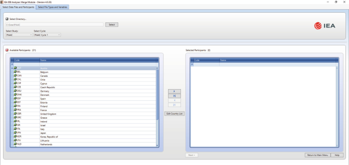

  

  IDB Analyzer merge module: select data files and participants

• 6. Click the countries of interest from the ‘Available Participants’ list and click the right arrow button (▹) to move them to the ‘Selected Participants’ panel on the right. Individual countries can also be moved directly to the ‘Selected Participants’ panel by double-clicking on them. To select multiple countries, hold the CTRL-key of the keyboard when clicking on countries. Click the tab-right arrow button (⊵) to move all countries to the ‘Selected Participants’ panel. For this example, we selected all the countries available.

• 7. Click the ‘Next >’ button to proceed to the next step. The software will open the ‘Select File Types and Variables’ tab of the merge module (see Fig. 6.3), to select the file types and the variables to be included in the merged data file.

• 8. Select the files for merging by checking the appropriate boxes to the left of the window. For example, in Fig. 6.3, the ‘General Response File’ has been selected.⁵ Checking this box will automatically populate the ‘Selected Variables’ panel with the three scores available in PIAAC (i.e. Literacy Scale Score, Numeracy Scale Score, and Problem-Solving Scale Score), as well as with all the ID (e.g. Country ID) and sampling variables (e.g. sampling and replicate weights) needed for the corresponding analyses (Fig. 6.4).

Fig. 6.3

IDB Analyzer merge module: selecting all countries

Fig. 6.4

IDB Analyzer merge module: select data files and participants

• 9. Select the variables of interest from the ‘Available Variables’ list in the left panel. In SPSS, you can right-click on the variable names to open a menu with details about each of the available variables (i.e. variable name, label, measurement level, and value labels). Variables are selected by clicking on them and then clicking the right arrow (▹) button. Clicking the tab-right arrow (⊵) button selects all variables (Fig. 6.5).

  Fig. 6.5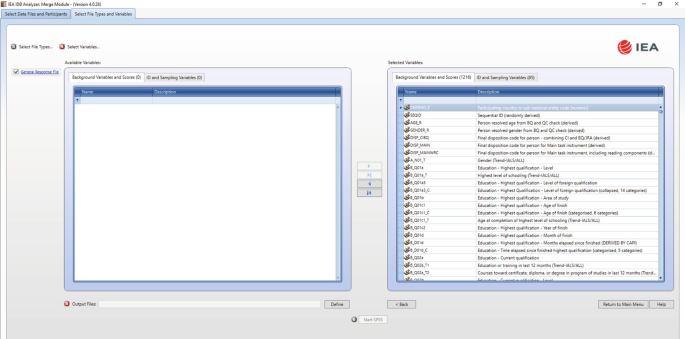

  

  IDB Analyzer merge module: selecting all variables

• 10. When selecting the variables, you can search variables by variable name or by variable label using the filter boxes (blue space between column header and list of variables) in the ‘Available Variables’ list and ‘Selected Variables’ list.

• 11. Note that the IDB Analyzer assumes that files have the same structure and the variables have the same properties (e.g. variables, formats, labels) in each of these files. Any deviation from this can cause unexpected results. Should you want to modify the contents of a file for a country, or a set of countries, it is recommended to do this on the resulting merged file, after the merge is completed.

• 12. In the ‘Output Files’ field, click on the ‘Define’ button to specify the name for the merged data file and the folder where it will be saved. The IDB Analyzer will also create an SPSS syntax file (∗SPS) (or a SAS syntax file, ∗.SAS, if you are using this software) of the same name and in the same folder with the code necessary to perform the merge. In the example shown in Fig. 6.3, the merged data file ‘merge_piaac.sav’ and the syntax file ‘merge_piaac.sps’ both will be created and stored in the folder titled ‘C:\Data\’. The merged data file will contain all the variables listed in the ‘Selected Variables’ panel, and if all available variables were selected, the resulting merge file should be about 622 megabytes in size.

• 13. Click the ‘Start SPSS’ button to create the SPSS syntax file. An SPSS Syntax Editor window with the created syntax code will be automatically opened. The syntax file can be executed by opening the ‘Run’ menu of SPSS and selecting the ‘All’ menu option. Alternatively, you can also submit the code for processing with the keystrokes Ctrl+A (to select all), followed by Ctrl+R (to run the selection). In SAS, the syntax file can be executed by selecting the ‘Submit’ option from the ‘Run’ menu.

Once SPSS or SAS has completed its execution, it is important to check the SPSS output window or SAS log for possible warnings. If warnings appear, they should be examined carefully because they might indicate that the merge process was not performed properly and that the resulting merged data file might not include all the relevant variables or countries.

6.3 Example Analyses with the IDB Analyzer

In the following section, we will describe step-by-step instructions to produce means, percentiles, percentages, linear regressions, correlations, and benchmarks, using the latest PIAAC public-use data files. In each subsection, a sequence of steps will be included as a numbered list. These steps are reiterated for each analysis routine. In this way, each subsection is self-contained, and the reader does not need to consult any other part of the chapter to complete the steps she or he needs to follow to produce means, percentiles, percentages, linear regressions, correlations, or benchmarks.

6.3.1 Means with Plausible Values

In this section, we illustrate how to estimate the means of literacy scores by country. The first example contains a variable with plausible values. In PIAAC there are three variables with plausible values: the literacy scale scores, the numeracy scale score, and the problem-solving scale score. Each of these variables consists of ten different columns of values within the PIAAC dataset. For each test, plausible values are generated as random draws of the posterior distribution of the participant’s proficiency (Wu 2005). To produce population estimates with these scores, the IDB Analyzer computes the results for each plausible value and combines these estimates using Rubin-Shaffer rules (Rutkowski et al. 2010). The following steps produce mean estimates of literacy proficiency by country, for females and males:

• 1. Open the IDB Analyzer.

• 2. Select the statistical software you want to work with (choose between SAS or SPSS).

• 3. Open the Analysis Module of the IDB Analyzer.

• 4. For this example, specify the data file ‘merge_piaac.sav’ as the Analysis File (see Sect. 6.2 in this chapter for details on how this file was created).

• 5. Select ‘PIAAC (using final full sample weight)’ as the Analysis Type.

• 6. Select ‘Percentages and Means’ as the Statistic Type.

• 7. Under the ‘Plausible Values Options’, select ‘Use PVs’.

• 8. Click on the ‘Separate Tables by’ section at the right-hand side of the software window. This section will become active and highlighted in light yellow.

• 9. Go to the ‘Select variables’ section, and click on the ‘GENDER_R’ variable in the fourth row of the name list.

• 10. Drag the ‘GENDER_R’ variable to the ‘Separate Tables by’ section.

• 11. Click on the ‘Plausible Values’ section at the right-hand side of the software window. This section will become active and highlighted in light yellow.

• 12. Go to the ‘Select variables’ section and click on the ‘PVLIT1–10’ variable in the first row of the name list.

• 13. Drag the ‘PVLIT1–10’ variable to the ‘Plausible Values’ section.

• 14. The Weight Variable is automatically selected by the software. SPFTWT0 is selected by default; this variable contains the final sampling weight.

• 15. Specify the name and the folder of the output files in the ‘Output Files’ field by clicking the Define/Modify button. For this example, we use the term ‘mean_with_pv’.

After all these steps, the reached setup should look similar to Fig. 6.6:

Fig. 6.6

Analysis of means by group setup

• 16. Then, click the ‘Start SPSS’ button. This will create an SPSS syntax file and open it in an SPSS editor window.

• 17. To start the computations, one needs to press the following keys combinations: CTRL+A first, to select the entire generated code present in the syntax window, and then CTRL+R to run these commands. The output of these analyses is depicted in Fig. 6.7.

Fig. 6.7

Analysis of mean by group output

In the generated output, the first column contains the list of countries. The second column presents the categorical values of the ‘GENDER_R’ variable: ‘Male’ and ‘Female’. In the third column, the nominal sample size is presented for each group, within each country. In the fourth column, the sum of survey weights is included. These later numbers represent the survey population to which the estimates are projected (Heeringa et al. 2009). Additionally, the IDB Analyzer generates standard errors for the survey population size (sixth column). In the ‘Percent’ column, the estimate of the proportion of each group in the population is presented. These point estimates are accompanied by their standard errors in the ‘Percent (s.e.)’ column. In the column ‘PVLIT (Mean)’, we find the point estimates of the literacy scores. Each country has two values, one for males and one for females. These point estimates present uncertainty, due to measurement error and due to sampling error. This uncertainty is summarised in the ‘PVLIT (s.e.)’ column. Standard deviations of these means are included in the ‘Std.Dev’ column. Similarly to previous estimates, on its right, standard errors of the standard deviations are provided in the column ‘Std.Dev. (s.e.)’. Finally, the last column, ‘pctmiss’, contains the percentage of missing cases in the variables involved in the analysis (‘PVLIT1-10’ and ‘GENDER_R’).

The IDB Analyzer creates six files after an analysis of means with plausible values is complete. Table 6.1 details these files and their content.

Table 6.1 Generated files by an analysis of means

Using the results provided in the file ‘means_with_pvGENDER_R.xlsx’, we created Table 6.2 to present the computed results. Means are presented and their standard errors are included in parenthesis.

Table 6.2 Means of literacy scores for female and males in each country

The IDB Analyzer produces a ‘Table Average’, which contains an overall mean between all countries, with its standard error. These estimates are presented in Table 6.2 in the last row, in the second column. The illustrated routine can be replicated with the numeracy scale scores and with the problem-solving scores present in PIAAC study.

6.3.2 Means with Other Variables

In the following example, which is simpler than its previous counterpart, we compute the mean of total years of schooling in each country. In the PIAAC study, total years of schooling was derived using different responses of participants regarding their educational participation during their lifetime. These values can be found in the ‘YRSQUAL_T’ variable. Using the IDB Analyzer, we need to follow the next steps:

• 1. Open the IDB Analyzer.

• 2. Select the statistical software you want to work with (choose between SAS or SPSS).

• 3. Open the Analysis Module of the IDB Analyzer.

• 4. For this example, specify the data file ‘merge_piaac.sav’ as the Analysis File (see Sect. 6.2 in this chapter for the details of how this file was created).

• 5. Select ‘PIAAC (using final full sample weight)’ as the Analysis Type.

• 6. Select ‘Percentages and Means’ as the Statistic Type.

• 7. Under the ‘Plausible Values Options’, select ‘None Used’.

• 8. Click on the ‘Analysis Variables’ section at the right-hand side of the software window. This section will become active and highlighted in light yellow.

• 9. Go to the ‘Select variables’ section, and under the ‘Description’ heading click on it, and type in ‘total years’. This action would look for all the variables containing ‘total’ and ‘year’ in their description field.

• 10. Specify the variable YRSQUAL_T as the analysis variable by clicking the ‘Analysis Variables’ field to activate it. Select YRSQUAL_T from the list of available variables present in the ‘Select Variables’ section and move it to the ‘Analysis variables’ by clicking the right arrow button in this section.

• 11. The Weight Variable is automatically selected by the software. SPFTWT0 is selected by default; this variable contains the final sampling weight.

• 12. Specify the name and the folder of the output files in the ‘Output Files’ field by clicking the Define/Modify button. For this example, we use the term ‘mean’.

After all these steps, the reached setup should look similar to Fig. 6.8:

Fig. 6.8

Analysis of means setup

• 13. Then, click the ‘Start SPSS’ button. This will create an SPSS syntax file and open it in an SPSS editor window.

• 14. To start the computations, one needs to press the following key combinations: CTRL+A first, to select the entire generated code present in the syntax window, and then CTRL+R to run these commands. The output of these analyses is depicted in Fig. 6.9.

Fig. 6.9

Analysis of means output

Similar to the previous example, the generated output presents several columns. The first column is the list of countries. In the second column is the nominal sample size of each country. Notice that Austria and Germany do not have observations for this variable and present 100% of missing. The third column contains the sum of survey weights, which represents the survey population size (Heeringa et al. 2009), and in the fourth column, the IDB Analyzer includes the standards errors of the survey population size. In the ‘Percent’ column, the proportion of the survey population size is depicted. For example, the United States projects its number of cases (4286) to a survey population of more than 166 million people, and its resulting proportion in the table is of ‘24,13’, whereas Canada has a larger nominal sample of 26,472 cases, yet projected to a survey population of more than 23 million people, and hence its proportion in the table is of ‘3,37’. These percentages are accompanied by their standard errors included in the sixth column. In the seventh column, the estimates of interest are included: the mean of total years of schooling per country, under the heading ‘YRSQUAL_T (Mean)’. Next to it, in the eighth column, we find the standard errors of these estimates, below the heading ‘YRSQUAL_T (s.e.)’. The ‘Std.Dev’ column contains the standard deviations of the analysis variable, and the ‘Std.Dev (s.e.)’ contains the standard deviations standard errors. The last column of the table presents the percentage of missing values of the analysed variable.

When the analysis of means is complete, the IDB Analyzer generates six files. Table 6.3 details these files and their content.

Table 6.3 Generated files by an analysis of means

Using the results provided in the file ‘mean.xlsx’, we created Table 6.4 to present the computed results.

Table 6.4 Means of lifetime years of schooling

Considering that the population average might not be the most informative location parameter to describe the variable’s distribution, in the next section we describe how to obtain percentiles of a continuous variable.

6.3.3 Percentiles

Means and percentiles are different location parameters in a distribution (Wilcox 2017). The arithmetic mean is the expected location of the value with the least difference to the rest of the values within a distribution. In contrast, percentiles are any location under which there is a certain proportion of cases. Means are informative for symmetric distributions, such as the normal distribution. However, when distributions depart from normality, medians (50th percentile) or other location parameters could be of interest. For the following example, we choose the 25th, 50th, and 75th percentile for the same variable. We will repeat Steps 1–3 from the previous routine, but we will change the statistic type.

• 1. Open the Analysis Module of the IDB Analyzer.

• 2. For this example, specify the data file ‘merge_piaac.sav’ as the Analysis File (see Sect. 6.2 in this chapter for the details of how this file was created).

• 3. Select ‘PIAAC (using final full sample weight)’ as the Analysis Type.

• 4. Select ‘Percentiles’ as the Statistic Type.

• 5. Under the ‘Plausible Values Options’, select ‘None Used’.

• 6. Click on the ‘Analysis Variables’ section on the right-hand side of the software window. This section will become active and highlighted.

• 7. Go to the ‘Select variables’ section, and under the ‘Description’ heading, click on it, and type in ‘years’. This action would look for all the variables containing ‘years’ in their description field.

• 8. Specify the variable YRSQUAL_T as the analysis variable by clicking the ‘Analysis Variables’ field to activate it. Select YRSQUAL_T from the list of available variables present in the ‘Select Variables’ section, and move it to the ‘Analysis variables’ by clicking the right arrow button in this section. In this step, it is also possible to select more than one variable in this routine. However, for the sake of simplicity, in this example, we are including only one variable.

• 9. In the ‘Percentiles’ section, type in ‘25 50 75’, all separated by a space.

• 10. Specify the name and the folder of the output files in the ‘Output Files’ field by clicking the ‘Define/Modify’ button. For this example, we use the term ‘percentile’.

The generated setup should be similar to the screenshot presented in Fig. 6.10.

Fig. 6.10

Percentile setup

• 11. Afterwards, click the ‘Start SPSS’ button, run the syntax, and wait for the results to appear in the output window. The output from this routine is presented in Fig. 6.11

  Fig. 6.11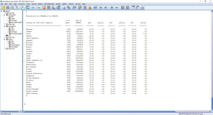

  

  Percentile output

The generated output presents nine columns. The first is the list of countries; the second is the nominal sample size for each country; and in the third column, we find the sum of survey weights, which represents survey population size (Heeringa et al. 2009). In the ‘Percent’ column, the IDB Analyzer includes the proportion that the survey population size represents within the output table. Then, for each requested percentile (p25, p50, p75), we can find the point estimates, and its standard error on its right (p25_se, p50_se, p75_se).

For the computation of percentiles, the IDB Analyzer generates four files. Table 6.5 details these files and their content.

Table 6.5 Generated files by an analysis of percentiles

Using the results provided in the file ‘percentile.xlsx’, we created Table 6.6 to present the computed results. The estimated percentiles are included for each country, alongside their standard errors in parenthesis.

Table 6.6 Percentiles (25th, 50th, and 75th) for total years of schooling by country

From the generated results, we notice that most of the participating countries have a median lifetime of schooling of 12 years. Ireland, the Netherlands, and Norway reach at least 14 years of schooling for half of their population of participants. At the lower end, Italy and Turkey presented a median schooling lifetime of 8 years.

6.3.4 Percentages

In the next example, we will create a new variable, not present in the merged files, to then retrieve percentage estimates at the population level for each country. We will use PIAAC data to estimate the proportion of the population in each participating country that has reached at least upper secondary education. To do this, we first need to recode a derived variable present in the public use file of the study. We will recode variable EDCAT8 into a dummy variable. EDCAT8 contains codes from the International Standard Classification of Education (ISCED) to express the highest level of formal education of the participants (OECD 2015).

Using the following syntax code (see Table 6.4), we can create a dummy variable that differentiates between the participants who hold an upper secondary qualification (coded as one) and the participants who present lower educational qualifications, such as a primary school qualification or an incomplete secondary school qualification (coded as zero).

To include this new variable in the generated merged file, the user needs to open the merged file in SPSS. Then, open a new syntax window; type in the syntax code included in Code 6.1; press CTRL+A and CTRL+R to create this variable. Click on the window with the merged data, and press CTRL+S to save this variable in the merged file.

Code 6.1: Recoding Highest Educational Level to a Dummy Variable

if (EDCAT8 <= 2) edu_usl = 0 .

if (EDCAT8 >= 3) edu_usl = 1 .

execute .

VARIABLE LABELS edu_usl 'Population with upper secondary education (1=yes, 0=no)'.

VALUE LABELS edu_usl

0 'No'

1 'Yes'.

With the merged file closed, one can open the IDB Analyzer and use this new variable for further analysis. In the next example, we will estimate what proportion of the population of the participant countries has at least upper secondary educational qualifications. Similarly to previous examples, we start by opening the IDB Analyzer:

• 1. Open the Analysis Module of the IDB Analyzer.

• 2. For this example, specify the data file ‘merge_piaac.sav’ as the Analysis File (see Sect. 6.2 in this chapter for the details on how this file was created).

• 3. Select ‘PIAAC (using final full sample weight)’ as the Analysis Type.

• 4. Select ‘Percentages only’ as the Statistic Type.

• 5. Click on the ‘Grouping Variables’ section.

• 6. Go to the ‘Select variables’ section, and under the ‘Description’ heading, click on it, and type in ‘upper’. This action would look for all the variables containing ‘upper’ in their description field. This is presented in Fig. 6.12.

  Fig. 6.12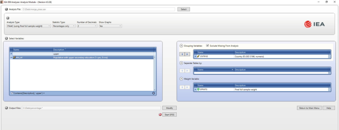

  

  Selecting a newly generated variable

• 7. Drag the variable ‘edu_usl’ to the ‘Grouping variable’ section. By clicking the ‘Analysis Variables’ field to activate it, select ‘edu_usl’ from the list of available variables present in the ‘Select Variables’ section, and move it to the ‘Grouping Variables’ field by clicking the right arrow button in this section.

• 8. Specify the name and the folder of the output files in the ‘Output Files’ field by clicking the ‘Define/Modify’ button. In this example, we will use the term ‘percentage’. This setup is presented in Fig. 6.13.

  Fig. 6.13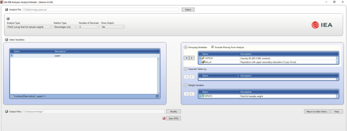

  

  Percentage setup

• 9. Click the ‘Start SPSS’ button to create the SPSS syntax file and open it in an SPSS editor window.

• 10. After the user has executed the generated syntax, by pressing the sequence of keys CTRL+A and CTRL+R, the IDB Analyzer will start to run their macros to compute the requested percentages.

Fig. 6.14

Percentage output

Once the calculations are finished, the SPSS output window would present the following results (see Fig. 6.14).

Similarly to the procedure of means estimation, the procedure to estimate percentages produces six files as outputs. These files and their contents are described in Table 6.7.

Table 6.7 Generated files by percentage analysis

Inspecting the generated output file in excel format, ‘percentage.xlsx’, we can filter and order the results to produce Table 6.8 and display the proportions of participants without upper secondary education for each participating country in PIAAC.

Table 6.8 Proportion of participants without upper secondary education

In the following section, we will use the dummy variable we have created, ‘edu_usl’, and estimate its relation to literacy scores in the population of each country.

6.3.5 Linear Regression

Apart from descriptive estimates such as means, percentiles, and percentages, the IDB Analyzer can also estimate regression models and logistic regression models (IEA 2019). In the following example, we will estimate the relationships between educational qualifications and literacy in each country. Specifically, we will estimate the gap in literacy scores between those who have at least an upper secondary education and the rest of the population. Although this gap can be obtained with a mean comparison, we want to retrieve more estimates than the mean differences between the two groups. We will use the linear regression routine for these purposes and get this difference as a standardised effect while also retrieving a measure of explained variance. These results can answer the question of ‘how much difference in literacy skills is there between those with and without upper secondary education?’. To estimate a regression analysis, we need to follow the next steps in the IDB Analyzer:

• 1. Open the Analysis Module of the IDB Analyzer.

• 2. For this example, specify the data file ‘merge_piaac.sav’ as the Analysis File (see Sect. 6.2 in this chapter for the details of how this file was created).

• 3. Select ‘PIAAC (using final full sample weight)’ as the Analysis Type.

• 4. Select ‘Regression’ as the Statistic Type.

• 5. Under the ‘Plausible Values Options’, select ‘Use PVs’.

• 6. On the right-hand side of the window, click on the area of ‘Dependent variables’. This will become highlighted once it is clicked.

• 7. Then, select ‘Plausible Values’ in the right-hand side window.

• 8. Move the cursor to the left-hand side of the window and click on the ‘PVLIT1–10’ variable to select the literacy scores.

• 9. Go back to the right-hand side and click on the right arrow to move the ‘PVLIT1–10’ variables, to the ‘Dependent Variables’ section.

• 10. Move the cursor to the ‘Independent Variables’ section, and click on the ‘Categorical Variables’ to activate this section.

• 11. Move the cursor to ‘Select Variables’ section on the left. Just right before the variable list, in the first row under the description section, type in ‘upper’. This will filter all present variables from the merged file.

• 12. Select the variable ‘edu_usl’, and move it to the right-hand side, by clicking on the right arrow, under ‘Independent Variables’, specifically using the right arrow from the ‘Categorical Variables’ subsection.

• 13. Specify the name and the folder of the output files in the ‘Output Files’ field by clicking the ‘Define/Modify’ button. In this example, we will name the syntax file as ‘regression’.

Once all these steps have been completed, the regression setup should look like Fig. 6.15.

Fig. 6.15

Regression setup

• 14. Click the ‘Start SPSS’ button. This action will open SPSS and create the syntax to run the regression model.

• 15. To execute the generated syntax, select all the written commands in the syntax editor, and run these commands using the ‘Run Selection’ button. Alternatively, press CTRL+A, to select all the commands, and then press CTRL+R to execute the syntax. This action would make SPSS run the regression analysis.

Because this analysis involves plausible values, it may take considerably longer in comparison with examples without plausible values in their calculations. This is because the regression analysis needs to be computed for each plausible value once, and then these results are synthetically presented using Rubin–Shaffer rules (Rutkowski et al. 2010). As such, this routine may take ten times longer than a regression analysis without the use of plausible values.

Once the regression analysis is done, SPSS will present the results in its output window. Figure 6.16 depicts how these results are displayed.

Fig. 6.16

Regression output

Once the analysis is concluded, the IDB Analyzer will generate eight files. These files include the syntax, the output, the model fit, the coefficients of the regression, and the descriptives of the included variables in the model. Table 6.9 lists the eight generated files and provides a description of their contents.

Table 6.9 Files generated by a regression analysis

Using the estimates present in ‘regression_Coef.xlsx’ and in ‘regression_Model.xlsx’, we created Table 6.10, to show at a glance the general results of the fitted model. These results are ranked in descending order using the R², a measure of explained variance (see, e.g. Field 2013, for more information about regression analysis).

Table 6.10 Standardised regression coefficients and model fit

Inspecting the regression coefficients present in ‘regression_Coef.xlsx’ and their t-values, we can conclude that all estimated differences are above the sampling error and all beta.t are larger than two. Thus, in all countries, those who have at least upper secondary education obtain higher literacy scores in the PIAAC test. The average difference of all participating countries is 0.32 standard deviations of literacy scores. The estimated gap varies between countries. For example, in Singapore, Spain, and Chile, it is larger than 0.45 standard deviations. In contrast, in Lithuania, the Russian Federation, and Poland, this difference is less than or equal to 0.16 standard deviations of literacy scores.

6.3.6 Correlations

In the PIAACe study, literacy, numeracy, and problem solving in technology-rich environments were measured. How are these different skills related to each other? In other words, to what extent do these three variables fluctuate together? In the OECD (2016a) report, ‘Skills Matter’, these variables were reported to be highly and positively correlated, with correlations of 0.86 for literacy and numeracy for the OECD partners (see, e.g. Field 2013, for more information about correlation analysis). In the following example, we will estimate the correlation between proficiency in literacy, numeracy, and problem solving in technology-rich environments. To compute these correlations, we need to follow the next steps:

• 1. Open the Analysis Module of the IDB Analyzer.

• 2. For this example, specify the data file ‘merge_piaac.sav’ as the Analysis File (see Sect. 6.2 in this chapter for the details of how this file was created).

• 3. Select ‘PIAAC (using final full sample weight)’ as the Analysis Type.

• 4. Select ‘Correlations’ as the Statistic Type.

• 5. Under the ‘Plausible Values Options’, select ‘Use PVs’.

• 6. Under the ‘Missing Data’ option, select ‘Pairwise’.

• 7. Click on the ‘Plausible Values’ section on the right-hand side of the software window.

• 8. Go to the ‘Select variables’ section, and select the three plausible values variables.

• 9. Move all the selected variables, by clicking the right arrow in the right-hand side window under the ‘Plausible Values’ subsection.

• 10. Specify the name and the folder of the output files in the ‘Output Files’ field by clicking the ‘Define/Modify’ button. In this example, we define the syntax as ‘correlation’.

The final setup should resemble the setup presented in Fig. 6.17.

Fig. 6.17

Correlation setup

• 11. Then, click the ‘Start SPSS’ button. This will create an SPSS syntax file and open it in an SPSS editor window.

• 12. To start the computations, one needs to press the following key combinations: CTRL+A first, to select the entire generated code present in the syntax window, and then CTRL+R to run these commands. The output of these analyses is depicted in Fig. 6.18.

Fig. 6.18

Correlation output

Because these computations involve the plausible values of the three proficiency scores, its estimation will take longer compared with correlations between variables with no plausible values. When the computations are done, six files are generated. These files are described in Table 6.11.

Table 6.11 Files generated by a correlation analysis

The output of these computations is displayed in Fig. 6.18.

These results match those shown in Table A2.7 of the report ‘Skills Matter: Further Results from the Survey of Adult Skills’ (OECD 2016a). In Table 6.12, we include only the matching countries from the OECD report, and the countries present in the current merged file. Thus, the correlations from Australia, Northern Ireland, and Jakarta (Indonesia) are excluded in the present table.

Table 6.12 Correlations between literacy and numeracy scale scores

6.3.7 Proficiency Levels

The PIAAC study presents proficiency levels—that is, segments of scores used to describe the skills of literacy, numeracy, and problem solving in technology-rich environments at different levels of ability. These are ranges of scores to describe in qualitative terms what participants can do at different levels of proficiency. In general terms, those participants with higher scores in each domain are more likely to resolve more difficult tasks than their counterparts with lower scores (OECD 2016a).

Literacy scale scores have six proficiency levels. These proficiency levels are briefly described in Table 6.13; more details can be found in ‘The Survey of Adults Skills: Reader’s Companion’ (OECD 2016b).

Table 6.13 Levels of proficiency

• 1. Open the Analysis Module of the IDB Analyzer.

• 2. For this example, specify the data file ‘merge_piaac.sav’ as the Analysis File (see Sect. 6.2 in this chapter for the details of how this file was created).

• 3. Select ‘PIAAC (using final full sample weight)’ as the Analysis Type.

• 4. Select ‘Benchmarks’ as the Statistic Type.

• 5. Under the ‘Benchmarks Options’ select ‘Discrete’. This option will retrieve what proportion of the population falls within each proficiency level. Other options include ‘Cumulative’, which computes the proportion of people at or above the cut score, and ‘Discrete with analysis variables’, which permits the user to calculate the mean of an analysis variable for those within each proficiency level. For this example, we will use the ‘Discrete’ option.

• 6. Click on the ‘Plausible Values’ section on the right-hand side of the software window.

• 7. Move the cursor to the left-hand side of the window and click on the ‘PVLIT1–10’ variable to select the literacy scores.

• 8. Move the selected variable, by clicking on the right arrow in the right-hand side window, under the ‘Plausible Values’ subsection.

• 9. Under the ‘Achievement Benchmarks’ section, select the corresponding scores for the literacy scores; these are ‘176 226 276 326 376’.

• 10. Specify the name and the folder of the output files in the ‘Output Files’ field by clicking the ‘Define/Modify’ button. Here we define the syntax as ‘benchmark’.

The setup of this analysis is depicted in Fig. 6.19.

Fig. 6.19

Benchmark setup

• 11. Click the ‘Start SPSS’ button. This action will open SPSS and create the syntax to run the regression model.

• 12. To execute the generated syntax, press CTRL+A to select all the commands, and then press CTRL+R to execute the syntax. Now, SPSS will compute the proportion of cases at each benchmark.

Results are displayed in Fig. 6.20, as they appear in SPSS.

Fig. 6.20

Benchmark output

What do these results mean? We need to consider the procedure the benchmark routine is doing to explain this output. Each cut score is the lower bound value for each defined range (IEA 2019). We used the following cut scores: ‘176 226 276 326 376’. Thus, it computes all the cases below 176 points, all the cases between 176 and 226, between 226 and 276, between 276 and 326, between 326 and 376, and finally all the cases above 376. In the last two columns of the output, the estimates are the percentage of cases and their standard errors that fall into the specified ranges. This procedure generates the following files in the specified location (see Table 6.14).

Table 6.14 Files generated by a correlation analysis

Using the information contained in ‘benchmark.xlsx’, we created Table 6.15. This table displays the proportions of participants who performed below Level 1 in the literacy proficiency scale.

Table 6.15 Percentage of participants below Proficiency Level 1

In Chile, 20% are below Level 1, whereas in Japan, Czech Republic, the Russian Federation, Cyprus, and the Slovak Republic, there are fewer than 2% below Level 1.

6.4 Concluding Remarks

In this chapter, we demonstrated how to perform both simple and complex analysis with PIAAC data using the IEA International Database (IDB) Analyzer. We showed examples of how to combine datasets from more than one country into a single data file for cross-country analyses. We also described and illustrated in a step-by-step fashion how to run descriptive statistical analyses, including means, percentiles, and percentages, as well as inferential analyses, such as correlations and regressions.

Although the examples included in this chapter used data from OECD’s PIAAC study, it is important to mention that the IDB Analyzer can be used to analyse not only PIAAC data but many other international large-scale assessments, such as the OECD’s PISA and TALIS studies, as well as, for example, IEA’s Trends in International Mathematics and Science Study (TIMSS), Progress in International Reading Literacy Study (PIRLS), and International Civic and Citizenship Study (ICCS).

The IDB Analyzer is certainly not the only tool available to obtain correct estimates when analysing PIAAC data, but it is probably the most user-friendly one. As mentioned before, the IDB Analyzer is a Windows-based tool that creates SAS code or SPSS syntax to perform analyses with PIAAC data. The code or syntax generated by the IDB Analyzer automatically takes into account the complex sample (e.g. sampling weights, replicate weights) and complex assessment design (e.g. plausible values) of PIAAC to compute analyses with the correct standard errors. It enables researchers to test statistical hypotheses in the population without having to write any programming code.

References

Field, A. (2013). Discovering statistics using IBM SPSS. London: Sage Publications.
Heeringa, S. G., West, B., & Berglund, P. A. (2009). Applied survey data analysis. Boca Raton: Taylor & Francis Group.
IBM. (2013). IBM SPSS statistics (Version 22.0). Somers: IBM corporation.
IEA. (2019). Help manual for the IEA IDB analyzer (Version 4.0). Hamburg, Germany. Retrieved from www.iea.nl/data.htm
OECD. (2015). Codebook for derived variables for PIAAC public database (with SAS code). Paris: OECD Publishing. Retrieved from http://www.oecd.org/skills/piaac/codebook for DVs 3_16 March 2015.docx.
OECD. (2016a). Skills matter: Further results from the survey of adult skills. Paris: OECD Publishing. https://doi.org/10.1787/9789264258051-en.
OECD. (2016b). The survey of adult skills: Reader’s companion. Paris: OECD Publishing. https://doi.org/10.1787/9789264204256-en.
Rutkowski, L., Gonzalez, E., Joncas, M., & von Davier, M. (2010). International large-scale assessment data: Issues in secondary analysis and reporting. Educational Researcher, 39(2), 142–151. https://doi.org/10.3102/0013189X10363170.
SAS. (2012). SAS system for windows (Version 9.4). Cary: SAS Institute.
Wilcox, R. R. (2017). Understanding and applying basic statistical methods using R. Hoboken: Wiley.
Wu, M. (2005). The role of plausible values in large-scale surveys. Studies in Educational Evaluation, 31(2–3), 114–128. https://doi.org/10.1016/j.stueduc.2005.05.005.
Author information
Authors and Affiliations
Corresponding author
Editor information
Editors and Affiliations
Rights and permissions
Open Access This chapter is licensed under the terms of the Creative Commons Attribution 4.0 International License (http://creativecommons.org/licenses/by/4.0/), which permits use, sharing, adaptation, distribution and reproduction in any medium or format, as long as you give appropriate credit to the original author(s) and the source, provide a link to the Creative Commons license and indicate if changes were made.
The images or other third party material in this chapter are included in the chapter's Creative Commons license, unless indicated otherwise in a credit line to the material. If material is not included in the chapter's Creative Commons license and your intended use is not permitted by statutory regulation or exceeds the permitted use, you will need to obtain permission directly from the copyright holder.
Copyright information
© 2020 The Author(s)
About this chapter
Cite this chapter
Sandoval-Hernandez, A., Carrasco, D. (2020). Analysing PIAAC Data with the IDB Analyzer (SPSS and SAS). In: Maehler, D., Rammstedt, B. (eds) Large-Scale Cognitive Assessment . Methodology of Educational Measurement and Assessment. Springer, Cham. https://doi.org/10.1007/978-3-030-47515-4_6
Download citation
DOI: https://doi.org/10.1007/978-3-030-47515-4_6
Published:
Publisher Name: Springer, Cham
Print ISBN: 978-3-030-47514-7
Online ISBN: 978-3-030-47515-4
eBook Packages: EducationEducation (R0)