A new method for image processing using generalized linguistic neutrosophic cubic aggregation operator

Abstract

Image processing is a technique of scrutinizing an image and extricating important information. Indecisive situations are generally undergone when the picture processes with profuse noise. Neutrosophic set (NS), a part of neutrosophy theory, studies the scope of neutralities and is essential to reasoning with incomplete and uncertain information. However, the linguistic neutrosophic cubic set (LNCS) is one of the extensions of the NS. In LNCS, each element is characterized by the interval-valued and single-valued neutrosophic numbers to handle the data uncertainties. Keeping these features in mind, we apply LNCS for image processing after defining their aggregation operators and operations. In this study, noisy grey-scale images were transformed into the LNCS domain using three membership degrees, then aggregated using aggregation operators. The proposed method clarifies the noise in the Lena image and three other test images. It has justified the utilization of operators based on visual clarity obtained. Suitable comparison analysis and efficiency testing is performed on the proposed theory by considering noise types, such as Gaussian, Poisson, and Speckle. In addition, we have also compared the computational efficiency of our proposed method with existing ones. The results show that our approach consumes less memory and executes quicker than the existing methods. A decision-maker can select a more effective operator to segment the images more effectively using the obtained results.

Introduction

Image processing is a branch in which an image serves as a piece of technical information providing entity holding a vast amount of information in the form of pixel values, dimensions and space used. For processing the information context contained by images, numerable tools and techniques are used to fit them into the desired framework of applicability. One such efficient method is to process the images using a fusion of information providing entities, such as pixels. However, aggregation operators (AOs) work adeptly in operating this information fusion.

Linguistic numbers are the best choice to measure the data in qualitative terms. Apparently, visual processing of the information can enhance the functionality of linguistic terms. Therefore, to combine the aspect of visual clarity, we have applied the proposed work in the field of image processing. The analysis of images involves a lot more optical clarity, and in such cases, we cannot rely on membership and non-membership solely, because noisy images are susceptible to a great deal of indeterminacy. Motivated by this, to analyze in a more detailed manner, we have contemplated the work under the LNCNs. Neutrosophic set is the better way to quantify an image, because subject to real-life scenarios, there may be an extent of indeterminacy in the images. For instance, the medical diagnosis images may not be apparent, or the images acquired from the CCTV footage may have many blur pixels. This aspect uncertainty quantifies by neutrosophic sets in which each pixel is categorized into three factors: the degrees of truth, the degree of falsity and the degree of indeterminacy. The proposed method is competent in aggregating the LNCSs with prospective applications in image processing. The method exhibits the efficient working of the proposed operators in processing the images with noise. It shows promising results by aggregating the noisy pixels of an image and displaying a better output image. The method enhances the visual clarity of the image and expresses the different working efficiencies of other proposed operators. For instance, it shows that edge detection can be done using linguistic neutrosophic cubic weighted Einstein or Hamachar geometric operators etc. With a number of operators proposed, the approach is suitable for various areas of image processing, including edge detection, feature extraction, background detailing, and so on. We have attempted to connect the linguistic scale to the visual variation of color from black to white in connection to it. For instance, in Fig. 1, the color corresponding to 0 is black, and that to 1 is white being passed through various shades of grey in-between. The assignment of discrete linguistic values, such as ‘black’, ‘light black’, ‘light grey’, ‘very light grey’, ‘extremely light grey’ and so on, would significantly improve the ability of an image analyst to capture the particulars of picture regions more accurately. Thus, we have assigned the visual color-coded strip to the numerical scale to classify the shades of grey correspondingly the numerical elements, to give a profound idea of the color variation from black to white.

Fig. 1

Linguistic scale with visual clarity

The main objective of this work is to develop the generalized AOs and apply them to image processing to make it possible to visualize the behaviour of different operators. This goal depends on how efficient LNCS is and how many different AOs can be applied. To achieve it, the primary goals of our work are:

• (1) To utilize the inherited capabilities of LNCSs of having linguistic features and vast uncertainty capturing ability by proposing generalized AOs on it.

• (2) We present generalized linguistic neutrosophic cubic weighted average and geometric AOs denoted by GLNCWA and GLNCWG based on Archimedean norms.

• (3) To construct a fuzzy model and put forth a novel approach for applying the proposed operators in image processing.

• (4) To classify the particularized versions of the proposed generalized AOs in addressing different image processing modes, such as “feature extraction”, “background detailing”, “edge detection”, and so on.

• (5) Validate the superiority of the proposed approach against some of the existing studies and compare the noise handling capabilities of the proposed method.

For achieving the above-listed objectives, the manuscript divides into different folds as “Preliminaries” defines all the concerned definitions regarding NS, NCS and LNCSs. In “Generalized operational laws and aggregation operators for LNCNs”, we proposed the basic operational laws, including GLNCWA and GLNCWG aggregation operators. In “Application of the proposed operators to image processing”, we provide a novel approach based on the proposed operators along with an algorithmic description of converting crisp pixel readings into LNCSs. “Illustrative examples” gives a detailed explanation of the applicability of the proposed operators in image processing and also distinguishes between the working domain of each operator along with its superiority analysis and noise handling efficiency. Finally, a concrete concluded remarks are given in “Conclusions”. For more clarity on the organization of the paper, we are specifying the sectionwise distribution of the manuscript in Fig. 2.

Fig. 2

Structural representation of the manuscript

Literature review

Traditionally, the information context dealt with only crisp numbers, but an escalation in complexities brought an emergent need to expand the analysis from crisp to advanced versions of handling uncertainties. To capture the prevailing uncertainties, fuzzy sets (FSs) [1], intuitionistic fuzzy set (IFSs) [2], interval-valued IFS (IVIFS) [3] theories are successful attempts. Numerous researchers [4,5,6] investigated these environments by proposing several AOs. It is noticeable that neither the FS nor IFS considers the indeterminacy aspect associated with the persisting situation. To overcome this, Smarandache [7] came up with neutrosophic sets (NSs) by adding a new entity named the degree indeterminacy along with membership and non-membership degrees. After its appearance, a concept of interval-valued neutrosophic sets (INSs) [8] and single-valued neutrosophic sets (SVNSs) [9] was introduced to allow the decision-makers to process imprecise and vague information. Due to their significance, several researchers put their efforts to establish the concept of these NSs by proposing a series of information measures [10, 11]. In addition to these measures, we have seen that the operators used to aggregate the various preferences have an underlying effect of encapsulating the information into a single units. In connection to it, there are numerable attempts to propose various AOs under the neutrosophic environment [12,13,14,15,16].

However, in practical decision-making situations, it is sometimes difficult to present the available information by only framing it into one extended FS. Thus, there is a dire need to efficiently hybridize more than one fuzzy environments to handle the unprocessed pieces of uncertain information. Therefore, in [17], authors corroborated a hybrid environment called cubic set (CS) by merging only the truth degrees of the interval-valued FS and FS. Thus, this creation of CS is limited to for the problem solving. To increase the flexibility of CS, authors [18, 19] presented a generalized version of the cubic set, named as cubic intuitionistic fuzzy sets (CIFSs), by integrating the truth and falsity degrees. Furthermore, to cover up the aspect of uncertainty in the hybridization, neutrosophic cubic sets (NCSs) were corroborated by Ali et al. [20]. All these environments evaluate the decision-makers preferences in quantitative terms, i.e., by considering inputs in numerical data. Ye [21] developed a concept of linguistic neutrosophic cubic sets (LNCSs) facilitate qualitative information.

The neutrosophic theory is a well-known theory, and it plays a crucial part in image processing. Numerous researchers [22,23,24,25] have made use of the remarkable properties of the neutrosophic set in the field of image processing. Keeping in mind the benefits of LNCNs, we have proposed a method for image processing aligned to achieve the visual clarity of the proposed operators. Despite using many aggregation norms, there has always been a dilemma related to their situational applicability. There is no way to know which operator needs to be used at what point of time. The purpose of this paper is to explore the use and relevance of a variety of operators in an LNCS environment subjected to image processing. In contrast to the neutrosophic statistics [26], the current work has indeterminacy as a coinciding factor. In the proposed work, as well as in the neutrosophic statistics, indeterminacy plays a vital role. It can enhance the scope of analysis and help in-depth study practical situations. For instance, Chen et al. [27] analyzed the rock joint roughness coefficient based on neutrosophic sets. Aslam et al. [28] gave novel diagnosis tests under neutrosophic statistics for diabetic patients considering the aspect of indeterminacy into account. The current work also includes the indeterminacy factor in image processing.

Noise removal is an essential aspect of image processing. Many deep neural network (DNN) based algorithms and techniques can filter the noise. In the presented work, aggregation operators based on linguistic neutrosophic cubic sets are applied into the field of image processing. The main essence of the work lies in proposing an algorithmic approach for providing the visual clarity of the proposed operators under the LNCS environment. In the literature, various researchers have utilized the features of neutrosophic sets in image processing such as Arulpandy and Pricilla [29] has presented the salt and pepper noise reduction method based on neutrosophic sets. Similarly, Guo et al. [30] also proposed a new approach for image denoising based on the concept of neutrosophic information. On the other hand, under a neutrosophic environment, several researchers [31, 32] have contributed in proposing different aggregation operators. These pioneering researches provided no idea of the visual applicability of varying aggregation operators. So, it was always difficult for a decision-maker to decide the variability of the role of one aggregation operator from the other. In the presented work, we intend to propose a series of aggregation operators based on LNCS and specify their applicability in image processing to overcome this problem. For it, we established a theory involving both the neutrosophic aggregation operators and neutrosophic image processing. We addressed the different roles of proposed aggregation operators based on their visual clarity.

It is evident from the above contributions that a wealth of literature is available on AOs. However, the concern remains regarding the selection of the appropriate operator. To answer this question, we have proposed generalized AOs on LNCSs and investigated them by giving a novel approach to processing different test images. One such considered test image is the famous research-based image called Lena image. It is a standardized $512 \times 512$ pixel dimensionalized picture being used rigorously by the scientists as a test image for testing different image processing techniques. We have also incorporated the proposed AOs on three more test images, first for background detailing, second for edge detection and third one for the minute objects’s detailing. Throughout the literature, many contributions are made in testing various images. For instance, in [33], the authors proposed the fuzzy filtering techniques for mixed noise reduction and used the Lena image as the reference image to conduct their study. In [34], authors gave a fuzzy-based improved image enhancement algorithm and has provided all his test results on Lena image. Apart from it, aligning concepts of fuzzy sets to image processing, mainly based on the NSs, Mohan et al. [35] gave a method for neutrosophic image denoising. MRI denoising using Weiner operators has been done by Mohan et al. [36].Talouki et al. [37] presented a review on all the neutrosophic image processing techniques. In addition to it, [38] worked on edge detection. Guo et al. [39] presented an algorithm based on neutrosophic threshold techniques, while [40] gave a technique for image retriever and classifier. In addition, several image analysts [41,42,43] have developed algorithms for processing images based on collaborating fuzzy rules.

Preliminaries

In this section, we review some basic concepts on NS and linguistic variables over the set ${\mathcal {X}}$.

Definition 1

[44]. A NS (Neutrosophic set) ${\mathcal {N}}$ in ${\mathcal {X}}$ is defined as

$$\begin{aligned} {\mathcal {N}}= \left\{ x, T(x), I(x), F(x) \mid x \in {\mathcal {X}}\right\} \end{aligned}$$

(1)

where $T, I, F: {\mathcal {X}}\rightarrow ]^-0, 1^+[$ represents the acceptance, indeterminacy and the non-acceptance degrees with the condition that “$^-0 \le \sup {T}(x)+ \sup {I}(x)+ \sup {F}(x) \le 3^+$”, where $\sup$ denotes “supremum”.

Definition 2

[9, 44]. A SVNS ${\mathcal {N}}$ in ${\mathcal {X}}$ is stated as

$$\begin{aligned} {\mathcal {N}}= \left\{ (x, T(x), I(x), F(x)) \mid x \in {\mathcal {X}}\right\} \end{aligned}$$

(2)

where $T,I,F\in [0,1]$ and $0 \le T+I+F\le 3$. For convenience, we call a pair ${\mathcal {N}}= (T,I,F)$ as SVN number (SVNN).

Definition 3

[8]. An interval-valued NS ${\mathcal {N}}$ in ${\mathcal {X}}$ is defined as

$$\begin{aligned} {\mathcal {N}}= & {} \left\{ x, \left[ T^L(x), T^U(x)\right] ,\left[ I^L(x), I^U(x) \right] , \right. \nonumber \\&\quad \left. \left[ F^L(x), F^U(x) \right] \mid x \in {\mathcal {X}}\right\} \end{aligned}$$

(3)

where $\left[ T^L(x), T^U(x)\right] , \left[ I^L(x), I^U(x) \right] , \left[ F^L(x), F^U(x) \right] \subseteq [0,1]$ determine the truth, indeterminacy and falsity intervals such that, $0\le T^U(x) + I^U(x) + F^U(x)\le 3$.

The concept of the neutrosophic cubic set was developed by combining SVNSs and INSs as indicated in the following definition:

Definition 4

[20]. A neutrosophic cubic set (NCS) ${\mathcal {C}}$ in ${\mathcal {X}}$ is defined as

$$\begin{aligned} {{\mathcal {C}}=\left\{ x, {\mathcal {A}}(x),\uplambda (x)\mid x \in {\mathcal {X}}\right\} } \end{aligned}$$

(4)

where ${\mathcal {A}}(x)=(x, [T^L(x), T^U(x)], [I^L(x), I^U(x)], [F^L(x)$, $F^U(x)])$ is an INS and $\uplambda (x) = (x,T(x)$, I(x), $F(x) \mid x \in X )$ is a SVNS in ${\mathcal {X}}$.

For sake of simplicity, an element in NCS is represented as

$$\begin{aligned} {\mathcal {C}}=( ([T^L, T^U], [I^L, I^U], [F^L, F^U] ), (T,I,F )) \end{aligned}$$

and is called as neutrosophic cubic number (NCN), where $[T^L,T^U],[I^L,I^U],[F^L,F^U] \subseteq [0,1]$ and $0\le T,I,F \le 1$ satisfying the conditions $0 \le T^U+I^U+F^U\le 3$ and $0\le T+I+F \le 3.$

A linguistic variable (LV) [45] is defined as follows in terms of linguistic features.

Definition 5

[45]. Let $S=\big \{s_{v} \mid v=0,1,2,\ldots ,p \big \}$ with odd cardinality be a linguistic term set (LTS), where $s_{v}$ has the characteristics, such as

• (1) $s_{k}\le s_{v} \Leftrightarrow k\le v$

• (2) Negation$(s_{v}) = s_{p-v}$

• (3) $\max \{s_k,s_v\}=s_{\max (k,v)}$

• (4) $\min \{s_k,s_v\}=s_{\min (k,v)}$

Later on, Xu [46] defined the continuous LTS as

$$\begin{aligned} S_{[0,p]}=\{s_\alpha \mid s_0\le s_\alpha \le s_p, \alpha \in [0,p]\} \end{aligned}$$

Definition 6

[21]. Let $S=\{s_v \mid v \in [0,p] \}$, where $p+1$ is an odd number / cardinality. A LNCN ${\mathcal {L}}= \left( {\mathcal {A}}, \uplambda \right)$, where ${\mathcal {A}}=\left( [s_{T^L}, s_{T^U}],[s_{I^L}, s_{I^U}], [s_{F^L},s_{F^U}] \right)$ is an uncertain linguistic number with truth, indeterminacy and falsity linguistic variables for all $s_{T^L},s_{T^U},s_{I^L},s_{I^U},s_{F^L},s_{F^U} \in S$. Moreover, $T^L \le T^U, I^L \le I^U , F^L \le F^U,$ and $\uplambda =\left( s_T, s_I, s_F\right)$ is a linguistic neutrosophic number with truth, indeterminacy, falsity linguistic variables $s_T, s_I, s_F \in S$.

Noticeably, from Definitions 1 and 6, it is evident that NS and LNCS have a conceptual difference of the scope of consideration. For an element x, NS considers the truth degree, falsity, and indeterminacy. On the other hand, LNCS is the set that attaches the linguistic element to the NCS. LNCS is a more generalized format of NS and NCS incorporating the facility to the decision-maker to provide judgements in linguistic terms.

Definition 7

[21]. For LNCN ${\mathcal {L}}= \left( \left( \left[ s_{T^{L}} , s_{T^{U}} \right] , \left[ s_{I^{L}} , s_{I^{U}} \right] ,\right. \right. \left. \left. \left[ s_{F^{L}} , s_{F^{U}} \right] \right) , \left( s_{T}, s_{I} , s_{F} \right) \right)$, a score function is stated as

$$\begin{aligned} {\mathcal {S}}c\left( {\mathcal {L}}\right) = \frac{1}{9p}\left( \begin{aligned}&(4p+T^L+T^U - I^L - I^U - F^L - F^U) \\&\qquad + \left( 2p+T-I-F \right) \end{aligned} \right) \nonumber \\ \end{aligned}$$

(5)

and accuracy function is

$$\begin{aligned} {\mathcal {H}}\left( {\mathcal {L}}\right) = \frac{1}{3p}\left( \left( T^L+T^U-F^L-F^U \right) +\left( T-F \right) \right) \end{aligned}$$

(6)

Definition 8

[47]. A t-norm is defined as $N: [0,1] \times [0,1] \rightarrow [0,1],$ if it satisfies the conditions viz. boundary, monotonicity, commutativity and associativity, while a function $M(x,y)=1-N(1-x,1-y)$ is called t-conorm.

Definition 9

[47]. A function N (or M) is known as Archimedean t-norm (or t-conorm) if it is a continuous function and $N(x,x)<x$ $(\text {or } M(x,x)<x)$, for $x \in (0,1)$. It is said to be a strict Archimedean t-norm (t-conorm) if it increases strictly in $(0,1) \times (0,1)$. Furthermore, strict Archimedean t-norm (N) and t-conorm (M) can be expressed in form of continuous functions $a,b:(0,1]\rightarrow [0, \infty )$, respectively, as $N(x,y)= b^{-1}\big ( b(x)+b(y) \big )$ and $M(x,y)= a^{-1}\big ( a(x)+a(y) \big )$, where b is a decreasing function with $b(1)=0$; a is an increasing function with $a(0)=0$ and $b(x)=a(1-x)$.

Definition 10

Three color components typically represent an image: red (R), green (G) and blue (B). Images consists of pixels with values between (and including) 0 and 255. The luminance of every pixel varies from black to white, variating through different shades of grey. 0 represents the luminance of the ‘black’ pixel, and 255 represents the ‘white’ one.

Next, we have implemented the definitions according to the available literature, which targets the domain of fuzzy sets together with image processing.

Definition 11

[48]. Edge detection is the process to identify the edges of an image. The points where the image brightness diversifies sharply are named the edges (or boundaries) of the image. It is an important characteristic of an image to separate different regions. Sharp edges may be perceivable in an image with high contrast between different regions in it. A similar definition perspective has been defined by Guo and Sengur [24] under the neutrosophic environment.

Definition 12

[49]. Feature extraction is the process of describing or highlighting the relevant shape information contained in an image. Extracting the features is essential when you have a vast data set and require diminishing the irrelevant data without degrading any pertinent information. In addition, feature extraction accommodates to lessen the amount of unrelated data from the data set. Inline to it, Gaber et al. [50] have worked in utilizing the concept of feature extraction using neutrosophic sets.

Definition 13

[51, 52]. During processing noisy images, it is necessary to tackle the background detailing many times. The primary purpose of this processing is to detect the target object and clean the interior and exterior parts of the image to improve its appearance. In the current study, the test image “cameraman image” has been used to demonstrate it, as it has a vast background area captured that can be processed.

Definition 14

The minute object’s detailing is also one of the essential factors for image processing. In this process, a minute object needs to be identified. It includes specifying those areas of an image that are very thin or delicate in appearance. Such types of images processing are so crucial in many stages under several situations. For instance, image processing for detective purposes often rely on the processing image for the minute objects in it.

Generalized operational laws and aggregation operators for LNCNs

In this section, we define some generalized operational laws and the operators for LNCNs based on Archimedean t-conorm and t-norm (ATT) and state their properties.

Operational laws

The operations laws for LNCNs based on the ATT, are defined as follows.

Definition 15

Let ${\mathcal {L}}_i= (([s_{T_i^L}, s_{T_i^U} ] , [s_{I_i^L}, s_{I_i^U}], [s_{F_i^L}$, $s_{F_i^U}]), (s_{T_i}, s_{I_i}, s_{F_i} ) )$, $i=1,2$ and ${\mathcal {L}}= (([s_{T^L}, s_{T^U} ] ,$ $[s_{I^L} , s_{I^U}], [s_{F^L}, s_{F^U}])$, $(s_{T}$, $s_{I}$, $s_{F}) )$ are three LNCNs and a real number $\delta >0$. Then,

• (1)
  $$\begin{aligned}&{\mathcal {L}}_1 \oplus {\mathcal {L}}_2 = \left( \begin{aligned}&\left( \begin{aligned}&\left[ s_{f\left( T_1^L,T_2^L\right) }, s_{f(T_1^U,T_2^U)}\right] , \left[ s_{g(I_1^L, I_2^L)}, s_{g(I_1^U, I_2^U)}\right] , \\&\qquad \left[ s_{g(F_1^L, F_2^L)}, s_{g(F_1^U, F_2^U)}\right] \end{aligned} \right) , \left( \begin{aligned}&s_{f(T_1, T_2)}, s_{g(I_1, I_2)}, \\&\qquad s_{g(F_1, F_2)} \end{aligned} \right) \end{aligned} \right) \end{aligned}$$
• (2)
  $$\begin{aligned}&{\mathcal {L}}_1 \otimes {\mathcal {L}}_2 = \left( \begin{aligned}&\left( \begin{aligned}&\left[ s_{g(T_1^L,T_2^L)}, s_{g(T_1^U,T_2^U)}\right] , \left[ s_{f(I_1^L, I_2^L)}, s_{f(I_1^U, I_2^U)}\right] , \\&\qquad \left[ s_{f(F_1^L, F_2^L)}, s_{f(F_1^U, F_2^U)}\right] \end{aligned} \right) , \left( \begin{aligned}&s_{g(T_1, T_2)}, s_{f(I_1, I_2)}, \\&\qquad s_{f(F_1, F_2)} \end{aligned} \right) \end{aligned} \right) \end{aligned}$$

where $f(x,y)=a^{-1}(a(x)+a(y))$ and $g(x,y)=b^{-1}(b(x)+b(y))$

• (3)
  $$\begin{aligned}&\delta {\mathcal {L}} = \left( \begin{aligned} \left( \begin{aligned}&\left[ s_{a^{-1} (\delta a (T^L) )} , s_{a^{-1} (\delta a(T^U))} \right] , \left[ s_{b^{-1} ( \delta b(I^L ) )}, \right. \\&\left. s_{b^{-1} ( \delta b(I^U ) )} \right] , \left[ s_{b^{-1} ( \delta b(F^L ) )}, s_{b^{-1} ( \delta b(F^U ) )} \right] , \end{aligned} \right) ,\\ \left( \begin{aligned}&s_{a^{-1} \left( \delta a\left( T \right) \right) } , s_{b^{-1} \left( \delta b\left( {I} \right) \right) } , \\&\qquad s_{b^{-1} \left( \delta b\left( {F} \right) \right) } \end{aligned}\right) \end{aligned} \right) \end{aligned}$$
• (4)
  $$\begin{aligned}&{\mathcal {L}}^\delta = \left( \begin{aligned} \left( \begin{aligned}&\left[ s_{b^{-1} ( \delta b (T^L) )} , s_{b^{-1} ( \delta b(T^U) )} \right] , \left[ s_{a^{-1} ( \delta a(I^L ) )}, \right. \\&\left. s_{a^{-1} ( \delta a(I^U ) )} \right] , \left[ s_{a^{-1} ( \delta a(F^L ) )} , s_{a^{-1} ( \delta a(F^U ) )} \right] , \end{aligned} \right) ,\\ \left( \begin{aligned}&s_{b^{-1} \left( \delta b\left( {T} \right) \right) } , s_{a^{-1} \left( \delta a\left( {I} \right) \right) } , \\&\qquad s_{a^{-1} \left( \delta a\left( {F} \right) \right) } \end{aligned}\right) \end{aligned} \right) \end{aligned}$$

Theorem 1

For LNCNs ${\mathcal {L}}_i$’s and a real $\delta >0$, the operations defined in Definition 15 are also LNCNs.

Proof

Let ${\mathcal {L}}_3 = {\mathcal {L}}_1\oplus {\mathcal {L}}_2$ = $(([s_{T_3^L}, s_{T_3^U}], [s_{I_3^L}, s_{I_3^U}]$, $[s_{F_3^L}, s_{F_3^U}])$, $(s_{T_3}, s_{I_3}, s_{F_3}))$. Using Definition 15, we obtain $T_3^L = a^{-1}(a(T_1^L)+a(T_2^L))$, $T_3^U = a^{-1}(a(T_1^U)+a(T_2^U))$, $I_3^L = b^{-1}(b(I_1^L)+b(I_2^L))$, $I_3^U = b^{-1}(b(I_1^U)+b(I_2^U))$, $F_3^L = b^{-1}(b(F_1^L)+b(F_2^L))$, $F_3^U = b^{-1}(b(F_1^U)+b(F_2^U))$, $T_3 = a^{-1}(a(T_1)+a(T_2))$, $I_3 = b^{-1}(b(I_1)+b(I_2))$, and $F_3 = b^{-1}(b(F_1)+b(F_2))$. Using the nature of the parameters a and b mentioned in Definition 9, it is easily obtained that $0\le T_3^L,T_3^U, I_3^L, I_3^U, F_3^L, F_3^U, T_3, I_3, F_3 \le p$. Furthermore, $T_i^U+I_i^U+F_i^U\le 3p$ for $i=1,2$ and from the fact that the function a, b are increasing and decreasing, respectively, we get, ${\mathcal {L}}_1\oplus {\mathcal {L}}_2$ is LNCN. Similarly, we can prove for other parts. $\square$

Theorem 2

For LNCNs ${\mathcal {L}}$, ${\mathcal {L}}_1$, ${\mathcal {L}}_2$ and real numbers $\delta , \delta _1, \delta _2>0$, we have

• (1) ${\mathcal {L}}_1 \oplus {\mathcal {L}}_2 = {\mathcal {L}}_2 \oplus {\mathcal {L}}_1$

• (2) ${\mathcal {L}}_1 \otimes {\mathcal {L}}_2 = {\mathcal {L}}_2 \otimes {\mathcal {L}}_1$

• (3) $\delta \left( {\mathcal {L}}_1 \oplus {\mathcal {L}}_2 \right) = \delta {\mathcal {L}}_1 \oplus \delta {\mathcal {L}}_2$

• (4) $\left( {\mathcal {L}}_1 \otimes {\mathcal {L}}_2 \right) ^{\delta } = {\mathcal {L}}_1^{\delta } \otimes {\mathcal {L}}_2^{\delta }$

• (5) $\delta _1 {\mathcal {L}}\oplus \delta _2 {\mathcal {L}}= \left( \delta _1 + \delta _2 \right) {\mathcal {L}}$

• (6) ${{\mathcal {L}}}^{\delta _1} \otimes {\mathcal {L}}^{\delta _2} = {\mathcal {L}}^{\delta _1 + \delta _2}$

Proof

We shall prove parts (iii), while others can be followed in the similar way.

For $\delta >0,$ we have

$$\begin{aligned} \delta \left( {\mathcal {L}}_1 \oplus {\mathcal {L}}_2 \right)&= \delta \left( \begin{aligned} \left( \begin{aligned}&\left[ s_{a^{-1}\left( a(T_1^{L}) + a(T_2^{L}) \right) } , s_{a^{-1}\left( a(T_1^{U}) + a(T_2^{U}) \right) } \right] ,\\&\left[ s_{b^{-1}\left( b(I_1^{L}) + b(I_2^{L})\right) } , s_{b^{-1}\left( b(I_1^{U}) + b(I_2^{U}) \right) }\right] ,\\&\left[ s_{b^{-1}\left( b(F_1^{L}) + b(F_2^{L})\right) } , s_{b^{-1}\left( b(F_1^{U}) + b(F_2^{U})\right) } \right] \end{aligned}\right) , \left( \begin{aligned}&s_{a^{-1}\left( a(T_{1}) + a({T_{2}}) \right) } ,\\&s_{b^{-1}\left( b(I_{1}) + b({I_{2}}) \right) } ,\\&s_{b^{-1}\left( b(F_{1}) + b({F_{2}})\right) } \end{aligned}\right) \end{aligned} \right) \\&= \left( \begin{aligned}&\left( \begin{aligned}&\left[ s_{a^{-1} \left( \delta a \left( a^{-1}\left( a({T_1^{L}}) + a({T_2^{L}})\right) \right) \right) }, s_{a^{-1} \left( \delta a \left( a^{-1}\left( a({T_1^{U}}) + a({T_2^{U}}) \right) \right) \right) } \right] ,\\&\left[ s_{b^{-1} \left( \delta b \left( b^{-1}\left( b({I_1^{L}}) + b({I_2^{L}})\right) \right) \right) } , s_{b^{-1} \left( \delta b \left( b^{-1}\left( b({I_1^{U}}) + b({I_2^{U}}) \right) \right) \right) } \right] ,\\&\left[ s_{b^{-1} \left( \delta b \left( b^{-1}\left( b({F_1^{L}}) + b({F_2^{L}}) \right) \right) \right) } , s_{b^{-1} \left( \delta b \left( b^{-1}\left( b({F_1^{U}}) + b({F_2^{U}})\right) \right) \right) } \right] \end{aligned}\right) ,\\&\qquad \qquad \qquad \qquad \left( \begin{aligned}&s_{a^{-1} \left( \delta a \left( a^{-1}\left( a({T_{1}}) + a({T_{2}}) \right) \right) \right) } ,\\&s_{b^{-1} \left( \delta b \left( b^{-1}\left( b({I_{1}}) + b({I_{2}}) \right) \right) \right) } ,\\&s_{b^{-1} \left( \delta b \left( b^{-1}\left( b({F_{1}}) + b({F_{2}})\right) \right) \right) } \end{aligned}\right) \end{aligned} \right) \\&= \left( \begin{aligned}&\left( \begin{aligned}&\left[ s_{a^{-1} \left( \delta \left( a\left( {T_1^{L}}\right) + a\left( {T_2^{L}}\right) \right) \right) } , s_{a^{-1} \left( \delta \left( a\left( {T_1^{U}}\right) + a\left( {T_2^{U}}\right) \right) \right) } \right] ,\\&\left[ s_{b^{-1} \left( \delta \left( b({I_1^{L}}) + b({I_2^{L}}) \right) \right) } , s_{b^{-1} \left( \delta \left( b({I_1^{U}}) + b({I_2^{U}}) \right) \right) } \right] ,\\&\left[ s_{b^{-1} \left( \delta \left( b({F_1^{L}}) + b({F_2^{L}}) \right) \right) } , s_{b^{-1} \left( \delta \left( b({F_1^{U}}) + b({F_2^{U}}) \right) \right) } \right] \end{aligned}\right) , \left( \begin{aligned}&s_{a^{-1} \left( \delta \left( a\left( {T_{1}}\right) + a\left( {T_{2}}\right) \right) \right) },\\&s_{b^{-1} \left( \delta \left( b({I_{1}}) + b({I_{2}}) \right) \right) } ,\\&s_{b^{-1} \left( \delta \left( b({F_{1}}) + b({F_{2}}) \right) \right) } \end{aligned}\right) \end{aligned} \right) \\&=\delta {\mathcal {L}}_1 \oplus \delta {\mathcal {L}}_2 \end{aligned}$$

Proposed generalized linguistic operators

Let $\varOmega$ be the collection of LNCNs. Then, based on the defined operational laws, we describe some generalized aggregation operators on $\varOmega$ as follows:

Definition 16

For a collection of “n” LNCNs ${\mathcal {L}}_i$’s, a generalized linguistic neutrosophic cubic weighted average (GLNCWA) operator is a mapping $\text {GLNCWA} : \varOmega ^n \rightarrow \varOmega$ defined as

$$\begin{aligned} \text {GLNCWA}\left( {\mathcal {L}}_1, {\mathcal {L}}_2, \ldots , {\mathcal {L}}_n \right)&= \omega _1 {\mathcal {L}}_1 \oplus \omega _2 {\mathcal {L}}_2 \nonumber \\&\quad \oplus \ldots \oplus \omega _n {\mathcal {L}}_n \quad \end{aligned}$$

(7)

where $\omega _i$’s be the weight vector of ${\mathcal {L}}_i$ such that $\omega _i>0$ and $\sum _{i=1}^{n}\omega _i=1.$

Theorem 3

For “n” LNCNs ${\mathcal {L}}_i=(([s_{T_i^L}, s_{T_i^U}], [s_{I_i^L}$, $s_{I_i^U}], [s_{F_i^L}, s_{F_i^U}]), (s_{T_i},s_{I_i},s_{F_i}))$, the value obtained through Definition 16 is again an LNCN and is given as

$$\begin{aligned} \text {GLNCWA}\left( {\mathcal {L}}_1,{\mathcal {L}}_2,\ldots ,{\mathcal {L}}_n \right) = \left( \begin{aligned}&\left( \begin{aligned}&\left[ s_{a^{-1} \left( \sum \limits _{i=1}^{n} \omega _i a\left( T_i^L \right) \right) } , s_{a^{-1} \left( \sum \limits _{i=1}^{n} \omega _i a\left( T_i^U \right) \right) } \right] , \left[ s_{b^{-1} \left( \sum \limits _{i=1}^{n} \omega _i b\left( I_i^L \right) \right) } , \right. \\&\left. s_{b^{-1} \left( \sum \limits _{i=1}^{n} \omega _i b\left( I_i^U \right) \right) } \right] , \left[ s_{b^{-1} \left( \sum \limits _{i=1}^{n} \omega _i b\left( F_i^L \right) \right) } , s_{b^{-1} \left( \sum \limits _{i=1}^{n} \omega _i b\left( F_i^U \right) \right) } \right] \end{aligned}\right) , \\&\left( \begin{aligned} s_{a^{-1} \left( \sum \limits _{i=1}^{n} \omega _i a\left( {T_i} \right) \right) }, s_{b^{-1} \left( \sum \limits _{i=1}^{n} \omega _i b\left( {I_i} \right) \right) }, s_{b^{-1} \left( \sum \limits _{i=1}^{n} \omega _i b\left( {F_i} \right) \right) } \end{aligned}\right) \end{aligned} \right) \qquad \end{aligned}$$

(8)

Proof

By implementing the operational laws of LNCNs on Definition 16, Eq. (8) can be easily derived. $\square$

Definition 17

For “n” LNCNs ${\mathcal {L}}_i$, the generalized linguistic neutrosophic cubic weighted geometric (GLNCWG) operator is a mapping $\text {GLNCWG}:\varOmega ^n \rightarrow \varOmega$ defined as

$$\begin{aligned} \text {GLNCWG}\left( {\mathcal {L}}_1, {\mathcal {L}}_2, \ldots , {\mathcal {L}}_n \right) = \bigotimes _{i=1}^n ({\mathcal {L}}_i)^{\omega _i} \end{aligned}$$

(9)

where $\omega _i>0$, $\sum _{i=1}^n \omega _i=1$ is the weight vector of ${\mathcal {L}}_i$.

Theorem 4

The aggregated values of “n” LNCNs ${\mathcal {L}}_i$ using Definition 17 is again LNCN and is given by

$$\begin{aligned} \text {GLNCWG}\left( {\mathcal {L}}_1, {\mathcal {L}}_2,\ldots , {\mathcal {L}}_n \right) = \left( \begin{aligned}&\left( \begin{aligned}&\left[ s_{b^{-1} \left( \sum \limits _{i=1}^{n} \omega _i b\left( T_i^L \right) \right) } , s_{b^{-1} \left( \sum \limits _{i=1}^{n} \omega _i b\left( T_i^U \right) \right) } \right] , \left[ s_{a^{-1} \left( \sum \limits _{i=1}^{n} \omega _i a\left( I_i^L \right) \right) } , \right. \\&\left. s_{a^{-1} \left( \sum \limits _{i=1}^{n} \omega _i a\left( I_i^U \right) \right) } \right] , \left[ s_{a^{-1} \left( \sum \limits _{i=1}^{n} \omega _i a\left( F_i^L \right) \right) } , s_{a^{-1} \left( \sum \limits _{i=1}^{n} \omega _i a\left( F_i^U \right) \right) } \right] \end{aligned}\right) , \\&\left( \begin{aligned} s_{b^{-1} \left( \sum \limits _{i=1}^{n} \omega _i b\left( {T_i} \right) \right) }, s_{a^{-1} \left( \sum \limits _{i=1}^{n} \omega _i a\left( {I_i} \right) \right) }, s_{a^{-1} \left( \sum \limits _{i=1}^{n} \omega _i a\left( {F_i} \right) \right) } \end{aligned}\right) \end{aligned} \right) \qquad \qquad \end{aligned}$$

(10)

Proof

By implementing the operational laws of LNCNs on Definition 16, Eq. (10) can be easily derived. $\square$

The following numerical example illustrates the working of the proposed GLNCWG and GLNCWA operators.

Example 1

Let ${\mathcal {L}}_1=(([s_2,s_3], [s_3$, $s_5], [s_4, s_5]), (s_2, s_4, s_5))$, ${\mathcal {L}}_2=(([s_3, s_4], [s_2$, $s_3], [s_1, s_2])$, $(s_3, s_2, s_1))$, ${\mathcal {L}}_3=(([s_4, s_5], [s_5$, $s_6], [s_1, s_3])$, $(s_5, s_6, s_2))$ and ${\mathcal {L}}_4=(([s_2,s_4], [s_1,s_2], [s_3,s_4])$, $(s_3, s_2, s_4))$ be four LNCNs with $p=8$ and $\omega =(0.4, 0.2, 0.3, 0.1)^T$ be their associated weight vector. To implement the GLNCWA and GLNCWG operators, we utilize the ATT corresponding to $b(x)=-\log (x)$. Based on the given information, we compute

$$\begin{aligned} a^{-1}\left( \sum \limits _{i=1}^4 \omega _i a(T_i^L)\right)= & {} p\left( 1-\prod \limits _{i=1}^4\left( 1-T_i^L/p\right) ^{\omega _i}\right) \\= & {} 8\left( 1-\left( 1-2/8 \right) ^{0.4} \left( 1-3/8 \right) ^{0.2} \right. \\&\quad \left. \left( 1-4/8 \right) ^{0.3} \left( 1-2/8 \right) ^{0.1} \right) \\= & {} 2.8774 \end{aligned}$$

Similarly, we can obtain $a^{-1}\left( \sum _{i=1}^4 \omega _i a(T_i^U)\right) =3.9882$, $b^{-1}\left( \sum _{i=1}^4 \omega _i b(I_i^L)\right) = 2.8890$, $b^{-1}\left( \sum _{i=1}^4 \omega _i b(I_i^U)\right) = 4.3507$, $b^{-1}\left( \sum _{i=1}^4 \omega _i b(F_i^L)\right) {=} 1.9433$, $b^{-1}\left( \sum _{i=1}^4 \omega _i b(F_i^U)\right) = 3.4925$, $a^{-1}\left( \sum _{i=1}^4 \omega _i a(T_i)\right) = 3.3859$, $b^{-1}\left( \sum _{i=1}^4 \omega _i b(I_i)\right) = 3.6693$, $b^{-1}\left( \sum _{i=1}^4 \omega _i b(F_i)\right) = 2.6922$. Hence, by Eq. (8), we get

$$\begin{aligned}&\text {GLNCWA}({\mathcal {L}}_1, {\mathcal {L}}_2, {\mathcal {L}}_3, {\mathcal {L}}_4) \\&\quad = \left( \begin{aligned} \left( \begin{aligned} {}[s_{2.8774},s_{3.9882}], [s_{2.8890}, \\ s_{4.3507}], [s_{1.9433},s_{3.4925}] \end{aligned} \right) , \left( \begin{aligned}&s_{3.3859}, s_{3.6693}, \\&\qquad s_{2.6922} \end{aligned} \right) \end{aligned} \right) \\ \end{aligned}$$

Similarly, by Eq. (10), we get

$$\begin{aligned}&\text {GLNCWG}({\mathcal {L}}_1, {\mathcal {L}}_2, {\mathcal {L}}_3, {\mathcal {L}}_4) \\&\quad = \left( \begin{aligned} \left( \begin{aligned} {}[s_{2.6703},s_{3.8120}], [s_{3.3989}, \\ s_{4.8467}], [s_{2.5891},s_{3.8659}] \end{aligned} \right) , \left( \begin{aligned}&s_{2.9733}, s_{4.3307}, \\&\qquad s_{3.4968} \end{aligned} \right) \end{aligned} \right) \end{aligned}$$

Next, we investigate some properties of the GLNCWA and GLNCWG operators. Let $\omega _i>0$ be the normalized weight vector of ${\mathcal {L}}_i=(([s_{T_i^L}, s_{T_i^U}], [s_{I_i^L}, s_{I_i^U}], [s_{F_i^L}, s_{F_i^U}]), (s_{T_i}, s_{I_i}, s_{F_i}))$.

Property 1

If ${\mathcal {L}}_i = {\mathcal {L}}$ for all i, where ${\mathcal {L}}$ is another LNCN, then

$$\begin{aligned} \text {GLNCWA}({\mathcal {L}}_1, {\mathcal {L}}_2,\ldots , {\mathcal {L}}_n)={\mathcal {L}} \end{aligned}$$

Proof

Let ${\mathcal {L}}=(([s_{T^L}, s_{T^U}], [s_{I^L}, s_{I^U}], [s_{F^L}, s_{F^U}])$, $(s_{T}$, $s_{I}$, $s_{F}))$ be another LNCN. Since ${\mathcal {L}}_i = {\mathcal {L}}$ for all i which implies that $T_i^L={T}^L$, $T_i^U = {T}^U$ and so on. Thus, the terms $a^{-1} \left( \sum _{i=1}^{n} \omega _i a\left( T_i^L \right) \right) = a^{-1} \left( \sum _{i=1}^{n} \omega _i a\left( T^L \right) \right)$ = $a^{-1}\left( a(T^L)\right) = T^L$, $a^{-1} \left( \sum _{i=1}^{n} \omega _i a\left( T_i^U \right) \right) = a^{-1} \left( \sum _{i=1}^{n} \omega _i a\left( T^U \right) \right)$ = $a^{-1}\left( a(T^U)\right) = T^U$. Similarly, we get $b^{-1} \left( \sum _{i=1}^{n} \omega _i b\left( I_i^L \right) \right) = I^L$, $b^{-1} \left( \sum _{i=1}^{n} \omega _i b\left( I_i^U \right) \right) = I^U$, $b^{-1} \left( \sum _{i=1}^{n} \omega _i b\left( F_i^L \right) \right) = F^L$, $b^{-1} \left( \sum _{i=1}^{n} \omega _i b\left( F_i^U \right) \right) = F^U$, $a^{-1} \left( \sum _{i=1}^{n} \omega _i a\left( T_i \right) \right) = T$, $b^{-1} \left( \sum _{i=1}^{n} \omega _i b\left( I_i \right) \right) = I$, and $b^{-1} \left( \sum _{i=1}^{n} \omega _i b\left( F_i \right) \right) = F$. Hence, by Eq. (8), we get $\text {GLNCWA}({\mathcal {L}}_1, {\mathcal {L}}_2,\ldots , {\mathcal {L}}_n)={\mathcal {L}}$. $\square$

Property 2

Let ${\mathcal {L}}_i^* = (([s_{{T_i^*}^L}, s_{{T_i^*}^{U}}], [s_{{I_i^*}^{L}}, s_{{I_i^*}^{U}}], [s_{{F_i^*}^{L}}, s_{{F_i^*}^{U}}]), (s_{T_i^*}, s_{I_i^*}, s_{F_i^*}))$ be another LNCN satisfying $T_i^L \le {T_i^*}^L$, $T_i^U \le {T_i^*}^U$, $I_i^L \ge {I_i^*}^L$, $I_i^U \ge {I_i^*}^U$, $F_i^L \ge {F_i^*}^L$, $F_i^U \ge {F_i^*}^U$, ${T_i} \le {T_i^*}$, ${I_i} \ge {I_i^*}$, and ${F_i} \ge {F_i^*}$ for all i, then

$$\begin{aligned} \text {GLNCWA}({\mathcal {L}}_1, {\mathcal {L}}_2, \ldots , {\mathcal {L}}_n)\le \text {GLNCWA}({\mathcal {L}}_1^*, {\mathcal {L}}_2^*, \ldots , {\mathcal {L}}_n^*) \end{aligned}$$

Proof

Since $T_i^L \le {T_i^*}^L$ for all i and a, b are increasing and decreasing functions, therefore, for $T_i^L \le {T_i^*}^L$, $T_i^U \le {T_i^*}^U$, we have $a(T_i^L) \le a({T_i^*}^L)$, $a(T_i^U) \le a({T_i^*}^U)$. Now, for real number $\omega _i>0$, we have $\sum _{i=1}^n \omega _i a(T_i^L) \le \sum _{i=1}^n \omega _i a({T_i^*}^L)$, $\sum _{i=1}^n \omega _i a(T_i^U) \le \sum _{i=1}^n \omega _i a({T_i^*}^U)$. Hence, using increasing property of t-conorm, we get

$$\begin{aligned} a^{-1}\left( \sum \limits _{i=1}^n \omega _i a(T_i^L)\right) \le a^{-1}\left( \sum \limits _{i=1}^n \omega _i a({T_i^*}^L)\right) , \end{aligned}$$

and

$$\begin{aligned} a^{-1}\left( \sum \limits _{i=1}^n \omega _i a({T_i}^U) \right) \le a^{-1}\left( \sum \limits _{i=1}^n \omega _i a({T_i^*}^U)\right) \end{aligned}$$

Similarly, we can obtain that

$$\begin{aligned}&b^{-1}\left( \sum \limits _{i=1}^n \omega _i b({I_i}^L)\right) \ge b^{-1}\left( \sum \limits _{i=1}^n \omega _i b({I_i^*}^L)\right) , \\&\quad b^{-1}\left( \sum \limits _{i=1}^n \omega _i b({I_i}^U) \right) \ge b^{-1}\left( \sum \limits _{i=1}^n \omega _i b({I_i^*}^U)\right) , \\&b^{-1}\left( \sum \limits _{i=1}^n \omega _i b({F_i}^L)\right) \ge b^{-1}\left( \sum \limits _{i=1}^n \omega _i b({F_i^*}^L)\right) ,\\&\quad b^{-1}\left( \sum \limits _{i=1}^n \omega _i b({F_i}^U) \right) \ge b^{-1}\left( \sum \limits _{i=1}^n \omega _i b({F_i^*}^U)\right) , \\&a^{-1}\left( \sum \limits _{i=1}^n \omega _i b({T_i})\right) \le a^{-1}\left( \sum \limits _{i=1}^n \omega _i b({T_i^*})\right) ,\\&\quad b^{-1}\left( \sum \limits _{i=1}^n \omega _i b({I_i}) \right) \ge b^{-1}\left( \sum \limits _{i=1}^n \omega _i b({I_i^*})\right) , \\&\text {and} b^{-1}\left( \sum \limits _{i=1}^n \omega _i b({F_i}) \right) \ge b^{-1}\left( \sum \limits _{i=1}^n \omega _i b({F_i^*})\right) \end{aligned}$$

Hence, using the score function of LNCN, given in Definition 7, we get

$$\begin{aligned} \text {GLNCWA}({\mathcal {L}}_1, {\mathcal {L}}_2, \ldots , {\mathcal {L}}_n)\le \text {GLNCWA}({\mathcal {L}}_1^*, {\mathcal {L}}_2^*, \ldots , {\mathcal {L}}_n^*) \end{aligned}$$

$\square$

Property 3

Let ${\mathcal {L}}^- = (([s_{T^{L-}}, s_{T^{U-}}], [s_{I^{L+}}, s_{I^{U+}}], [s_{F^{L+}}, s_{F^{U+}}]), (s_{T^-}, s_{I^+}, s_{F^+}))$ and ${\mathcal {L}}^+ = (([s_{T^{L+}}, s_{T^{U+}}]$, $[s_{I^{L-}}$, $s_{I^{U-}}]$, $[s_{F^{L-}}$, $s_{F^{U-}}])$, $(s_{T^+}$, $s_{I^-}$, $s_{F^-}))$ where $s_{x^{y-}}=\min _i\{s_{x_i^y}\}$, $s_{x^{y+}}=\max _i\{s_{x_i^y}\}$, for $x\in \{T,I,F\}$ and $y\in \{L,U\}$. Then, we have ${\mathcal {L}}^- \le \text {GLNCWA}({\mathcal {L}}_1, {\mathcal {L}}_2, \ldots , {\mathcal {L}}_n)\le {\mathcal {L}}^+$.

Proof

Since ${\mathcal {L}}^- \le {\mathcal {L}}_i \le {\mathcal {L}}^+$ for all i, therefore, using above properties, we get

$$\begin{aligned}&\text {GLNCWA}({\mathcal {L}}^-, {\mathcal {L}}^-, \ldots , {\mathcal {L}}^-) \le \text {GLNCWA}({\mathcal {L}}_1, {\mathcal {L}}_2, \ldots , {\mathcal {L}}_n)\\&\quad \le \text {GLNCWA}({\mathcal {L}}^+,{\mathcal {L}}^+,\ldots ,{\mathcal {L}}^+) \end{aligned}$$

which implies that

$$\begin{aligned} {\mathcal {L}}^- \le \text {GLNCWA}({\mathcal {L}}_1, {\mathcal {L}}_2, \ldots , {\mathcal {L}}_n)\le {\mathcal {L}}^+. \end{aligned}$$

Hence, the result. $\square$

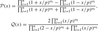
Furthermore, by assigning a different values of the generator $b:(0,1]\rightarrow [0,\infty )$, the proposed GLNCWA operator, given in Eq. (8), is particularized as

$$\begin{aligned}&\text {GLNCWA}\left( {\mathcal {L}}_1,{\mathcal {L}}_2,\ldots ,{\mathcal {L}}_n \right) \nonumber \\&\quad = \left( \begin{aligned} \left( \begin{aligned} {}[s_{p{\mathcal {P}}(T_i^L)}, s_{p{\mathcal {P}}(T_i^U)}], [s_{p{\mathcal {Q}}(I_i^L)}, \\ s_{p{\mathcal {Q}}(I_i^U)}], [s_{p{\mathcal {Q}}(F_i^L)}, s_{p{\mathcal {Q}}(F_i^U)}] \end{aligned} \right) , \left( \begin{aligned}&s_{p{\mathcal {P}}(T_i)}, s_{p{\mathcal {Q}}(I_i)}, \\&\qquad s_{p{\mathcal {Q}}(F_i)} \end{aligned} \right) \end{aligned} \right) \nonumber \\ \end{aligned}$$

(11)

here the function ${\mathcal {P}}$ and ${\mathcal {Q}}$ are defined according to the different functions b as

• (1) If $b(x)=-\log (x), x>0$, then

  $$\begin{aligned} {\mathcal {P}}(x)=1-\prod \limits _{i=1}^{n}\left( 1-x/p \right) ^{\omega _i} \text { and } {\mathcal {Q}}(x)= \prod \limits _{i=1}^{n} \left( x/p\right) ^{\omega _i} \end{aligned}$$

  and hence Eq. (11) is called as linguistic neutrosophic cubic weighted algebraic (LNCWA) operator.

• (2) If $b(x)=\log \left( \frac{2-x}{x} \right) ,$ then

  

  and hence Eq. (11) is called as linguistic neutrosophic cubic weighted Einstein averaging (LNCWEA) operator.

• (3) If $b(x)=\log \left( \frac{\gamma + (1-\gamma )x}{x}\right)$, $\gamma \in (0,\infty )$, then

  
  $$\begin{aligned} {\mathcal {Q}}(x)=\frac{\gamma \prod _{i=1}^{n} (x/p)^{\omega _i} }{\prod _{i=1}^{n}\left( 1+\left( \gamma -1 \right) (1-x/p) \right) ^{\omega _i} + \left( \gamma -1\right) \prod _{i=1}^{n} \left( x/p \right) ^{\omega _i} } \end{aligned}$$

  and hence Eq. (11) is called as linguistic neutrosophic cubic weighted hamachar average (LNCWHA) operator

Remark 1

The proposed LNCNWG operator also satisfies the properties of monotonicity, boundedness and idempotence for LNCNs, with their particular cases summarized similarly to above.

Application of the proposed operators to image processing

In this section, we demonstrate the application of the proposed operators to image processing. The benefit of use of fuzzy logic with that of image processing is an assimilation of various fuzzy approaches, which finally leads to the processed image. The objective of the problem is to fix random noise in the input image corresponding to its grey-scale equivalents of different color channels and aggregate them to process the image according to the need of the decision-maker. We have taken the noisy image and utilized the proposed AOs. As the taken image from the source always contains a lot of uncertainties, the decision-maker may be unable to make a decision accurately. To address it, there is a need for fuzzification onto the image, which convert the image’s pixels to a suitable fuzzy environment. Furthermore, each pixel is usually a real number, but conversion to the corresponding fuzzy number facilitates us to capture the extent of uncertainty in the sureness of the pixel value, as it is expected that, by properly addressing the noisy pixels and their fuzzification, the associated noise can be reduced. Therefore, to handle it, we convert the pixels of an image into LNCNs and process the input image using ‘imread()’ and ‘imshow()’ commands in the MATLAB image processing toolbar.

To completely deal with the uncertainty and process the image using the LNCNs, we state an algorithm whose phases are divided into three main stages: image acquisition, fuzzy model development and process of aggregation as well as defuzzification. The detailed description of each of the stages is described as below:

Phase 1: Image acquisition

The first stage of the approach is the image acquisition phase, where the image pixel data is read into the primary colors, namely, red, green and blue (RGB) channels. These color channels are so efficient that even the grey-scale equivalents of these color channels are used for clear representation of the objects in the image and various image detection algorithms. In the grey-scale, each pixel ranges between 0 to 255, where 0 represents the luminance of the pixel into black and 255 corresponds to the white visibility, while all the values ranging strictly between 0 and 255 show transition from white to black going through different intensities of grayness. Based on it, we took a noisy image at this acquisition stage, and capture the grey-scale pixel values $(r^{(N)}_{ij})$ corresponding to the ‘l’ number color channels in form of $m \times n$ matrices $C^{(N)}_{m \times n}$, where $i=1,2,\ldots ,m$; $j=1,2,\ldots ,n$; $N=1,2,\ldots ,l$, as

(12)

Phase 2: Development of the fuzzy model

For employing the aggregation process, we need to develop the suitable fuzzy model to which the norm operations are to be applied. Motivated by the wide uncertainty capturing capability of LNCNs, we are developing the fuzzy model in which each input pixel having a value belonging to the set of real numbers is converted into an LNCN. Aligning the utilization of LNCNs to image processing, certain guidelines in favor of the environment are followed. One such important consideration is that the cardinality should be between 0 (black color) to p (white color) through various shades of grey, as shown in Fig. 3, where the count 0 to 8 corresponds to $s_0$ to $s_8$. However, during the conversion stage, the pixels of the considered image are normalized using Eq. (13), in accordance to the cardinality ranging between 0 and p.

$$\begin{aligned} \text {Normalized pixel } (s_g) = s_{p * \left( \text {Noisy pixel}/255 \right) } \end{aligned}$$

(13)

Fig. 3

Linguistic scale

As the obtained normalized pixel of the image $s_g$ is too noisy, so there is a need to fuzzify it using the features of the LNCNs to handle the uncertainties in the image. To generate the membership and non-membership degrees of LNCNs from the normalized pixel $(s_g)$ and to widen the extent of pixel reading, we create the membership interval utilizing the greatest as well as the smallest integer value of g. Furthermore, it is noticeable that indeterminacy will also play a dominant role over here. By capturing the membership interval, it may be possible that the pixel reading is somewhat around the membership interval. For instance, if the normalized noisy pixel’s value is $s_g=s_{5.2},$ then using the greatest and smallest integer value of $s_g=s_{5.2}$, we considered the membership interval as $[s_5,s_6]$. To handle the indeterminacy degree around this membership interval $[s_5, s_6]$, we have taken a spread value denoted by ‘sp’, such that $sp \in {\mathbb {R}}$ with the condition that addition of the spread value should not make the linguistic variable to exceed the value p. Hence, $[s_{5+sp},s_{6+sp}],$ represent the indeterminacy interval. W.l.o.g. (Without loss of generality) in our model, we fix $sp=1,$ for the indeterminacy interval. However, taking into account the falsity values, it is evident that, if the actual pixel can be somewhere around or between $[s_5,s_6],$ then it can never be around the complemented value on the linguistic scale of it and hence non-membership interval is considered to be $[s_2,s_3]$. Hence, the formulated LNCN corresponding to pixel $s_g=s_{5.2}$ is obtained as $\left( \left( [s_5,s_6],[s_6,s_7],[s_2,s_3] \right) ,\left( s_{5.2},s_{6.2},s_{2.8} \right) \right) .$

With this idea, the following are key elements summarized during designing the LNCN from a given noisy pixel $s_c$ value.

• (i) If the noisy image contains a pixel value $s_c\in [s_{a_1},s_{a_2}],$ then $[s_{a_1},s_{a_2}]$ is called as membership interval and $s_c$ is the neutrosophic membership value.

• (ii) As the uncertainties always exist during the extraction of the information and hence these can be handled with the help of indeterminacy interval $[s_{a_1+1},s_{a_2+1}]$ and neutrosophic indeterminacy value as $s_d=s_{c+1}$ (for $sp=1$).

• (iii) The non-membership degree interval for the pixel $s_c$ is extracted as a complement w.r.t. the linguistic variable and get $s_{p-c}$. Hence, the non-membership pixel value and its corresponding falsity interval are given as $s_{p-c}$ and $[s_{p-a_2},s_{p-a_1}]$, respectively.

Keeping in mind the assumptions lined above, we formulate an Algorithm 1 for fuzzifying the noisy normalized image pixels to LNCNs. The input image has been taken as a noisy image and a random noise has been applied to it. For it, we have decided a spread value denoted as ‘sp’ in the Algorithm 1.

After implementing the Algorithm 1 to each real number pixel value in different color channel, we formulate the fuzzified decision matrices ${\mathcal {D}}^{(N)}=\left( {\mathcal {L}}^{(N)}_{ij}\right) _{m \times n}$ as

(14)

where ${\mathcal {L}}^{(N)}_{ij} = \left( \left( \left[ s^{(N)}_{T_{ij}^{L}}, s^{(N)}_{T_{ij}^{U}}\right] , \left[ s^{(N)}_{I_{ij}^{L}}, s^{(N)}_{I_{ij}^{U}}\right] , \left[ s^{(N)}_{F_{ij}^{L}}, s^{(N)}_{F_{ij}^{U}}\right] \right) , \right.$ $\left. \left( s^{(N)}_{T_{ij}}, s^{(N)}_{I_{ij}}, s^{(N)}_{F_{ij}}\right) \right)$ is an LNCN corresponding to each color image pixel $s_{g_{ij}}$.

Phase 3: Process of aggregation and defuzzification

After obtaining the information in terms of LNCNs for RGB channels, aggregate the matrices ${\mathcal {D}}^{(N)}=\left( {\mathcal {L}}^{(N)}_{ij} \right) _{m \times n}$ into a collective matrix ${\mathcal {D}}=\left( {\mathcal {L}}_{ij}\right) _{m \times n}$, where ${\mathcal {L}}_{ij}=(([s_{T_{ij}^L}, s_{T_{ij}^U}]$, $[s_{I_{ij}^L}$, $s_{I_{ij}^U}]$, $[s_{F_{ij}^L}$, $s_{F_{ij}^U}])$, $(s_{T_{ij}}$, $s_{I_{ij}}$, $s_{F_{ij}}))$, using the proposed AOs, namely, GLNCWA or GLNCWG with equal weighage to the information. For instance, using GLNCWA operator, we get

$$\begin{aligned}&{\mathcal {L}}_{ij} = \text {GLNCWA}\left( {\mathcal {L}}^{(1)}_{ij}, {\mathcal {L}}^{(2)}_{ij}, \ldots , {\mathcal {L}}^{(l)}_{ij} \right) = \left( \begin{aligned}&\left( \begin{aligned}&\left[ s^{(N)}_{a^{-1} \left( \sum \limits _{N=1}^{l} \omega _j a\left( (T_{ij}^{L}) \right) \right) } , s^{(N)}_{a^{-1} \left( \sum \limits _{N=1}^{l} \omega _j a\left( (T_{ij}^{U}) \right) \right) } \right] , \left[ s^{(N)}_{b^{-1} \left( \sum \limits _{N=1}^{l} \omega _j b\left( (I_{ij}^{L}) \right) \right) } , \right. \\&\left. s^{(N)}_{b^{-1} \left( \sum \limits _{N=1}^{l} \omega _j b\left( (I_{ij}^U) \right) \right) } \right] , \left[ s^{(N)}_{b^{-1} \left( \sum \limits _{N=1}^{l} \omega _j b\left( (F_{ij}^L) \right) \right) } , s^{(N)}_{b^{-1} \left( \sum \limits _{N=1}^{l} \omega _j b\left( (F_{ij}^U) \right) \right) } \right] \end{aligned}\right) , \\&\left( \begin{aligned} s^{(N)}_{a^{-1} \left( \sum \limits _{N=1}^{l} \omega _j a\left( T_{ij} \right) \right) }, s^{(N)}_{b^{-1} \left( \sum \limits _{N=1}^{l} \omega _j b\left( I_{ij} \right) \right) }, s^{(N)}_{b^{-1} \left( \sum \limits _{N=1}^{l} \omega _j b\left( F_{ij} \right) \right) } \end{aligned}\right) \end{aligned} \right) \nonumber \\ \end{aligned}$$

(15)

To defuzzify the process, we utilize the score value of the aggregated LNCNs by Eq. (5) as

$$\begin{aligned} {\mathcal {S}}c\left( {\mathcal {L}}_{ij}\right) =\frac{1}{9p}\left( \begin{aligned}&\left( 4p+T_{ij}^{L}+T_{ij}^{U} - I_{ij}^{L}-I_{ij}^{U}-F_{ij}^{L}-F_{ij}^{U}\right) \\&\qquad + \left( 2p+T_{ij}-I_{ij}-F_{ij} \right) \end{aligned} \right) \nonumber \\ \end{aligned}$$

(16)

Finally, based on these score values, the images are generated using ‘imshow()’ command in MATLAB image processing toolbar.

Fig. 4

Color channel matrices $C^{(1)}$, $C^{(2)}$ and $C^{(3)}$ corresponding to noisy grey-scale Lena image

Procedure of processing a noisy image—summarized steps

In a nutshell, we summarize the above explained procedure of processing a noisy image by aggregating its different color channels using the proposed AOs in the following steps:

• Step 1: By Eq. (12), formulate the matrices $C^{(N)}$ corresponding to ‘l’ different color channels of a noisy image.

• Step 2: Implement the Algorithm 1 to obtain the fuzzified matrices ${\mathcal {D}}^{(N)}$.

• Step 3: Aggregate the information of the matrices ${\mathcal {D}}^{(N)}$ into ${\mathcal {D}}$ using the proposed GLNCWA or GLNCWG operators.

• Step 4: Obtain the score value and their corresponding resultant image.

Illustrative examples

In this section, we examine the output in form of processed images obtained by following the steps in the proposed approach. For it, we have considered the four different test noisy images viz “Lena image”, “Cameraman image”, “Vegetable image” and “Chess-board image”. The proposed approach is based on aggregation operators based on the LNCS domain. The analysis is done on the basis of 4 test images and these test images are not chosen from a particular database. These images are taken into account, keeping in mind the following points:

• (i) The Lena image is used, because in that feature detection (based on the features of face) can be easily located visually.

• (ii) Cameraman image is used for understanding the behavior of the proposed method in the background detailing. For this, the image is considered, because it has wide background area that makes the analysis more convenient and easy to understand.

• (iii) Vegetable image is chosen intended to the analysis of edge detection. For it, each separating edge belonging to different object in the image, provide more clarity with better scope of analysis.

• (iv) Chessboard is considered to check the efficiency of the proposed method in the minute object detailing.

The proposed approach is demonstrated taking the case of “Lena image”. However, the approach is conducted on the three other images. The steps for each “Lena image” are demonstrated and to avoid the repetition of steps for each tested case the results and discussions for other images are discussed.

Case study

We, first, consider a noisy “Lena Image” and implement the proposed approach on it. This image is grey-scale image corresponding to composite of grey-scale images obtained from three color channels of the original image. On this input image, random noise is applied. By applying this noise, the scope of uncertainty of the original pixel is enhanced and noise capturing capability of LNCN is checked. The matrix corresponding to the Lena image is taken as $512 \times 512$ dimensioned, so to demonstrate the approach, we have shown the results, by figures, which represent $3 \times 3$ portion of the complete matrix of order 512. Then, the steps of the proposed approach in processing the Lena image are summarized as follows:

• Step 1: Consider the grey-scale equivalents of three color channels ($l=3$), namely, red, green and blue in which dimensions of each matrix are $512 \times 512$. Corresponding to it, the matrices $C^{(1)}, C^{(2)}$ and $C^{(3)}$ are obtained for the considering noisy Lena image which are shown in Fig. 4.

• Step 2: Normalize each pixel of the channel matrices using Eq. (13) and hence implemented the Algorithm 1 to obtain their corresponding LNCNs ${\mathcal {L}}_{ij}^{(1)}$, ${\mathcal {L}}_{ij}^{(2)}$ and ${\mathcal {L}}_{ij}^{(3)}$. The normalized values and their equivalent fuzzified channel matrices ${\mathcal {D}}^{(1)}$, ${\mathcal {D}}^{(2)}$ and ${\mathcal {D}}^{(3)}$ are shown in Fig. 5. For instance, after implementing the Algorithm 1, we obtain LNCNs as ${\mathcal {L}}^{(1)}_{11} = {\mathcal {L}}^{(1)}_{12}= (([s_7,s_8]$, $[s_6,s_7]$, $[s_0,s_1])$, $(s_{7.07}, s_{6.07}, s_{0.93}))$, ${\mathcal {L}}^{(1)}_{13} = (([s_5,s_6 ]$, $[s_6, s_7]$, $[s_2,s_3])$, $(s_{6.98}$, $s_{7.98}$, $s_{1.02}))$.

• Step 3: Aggregate these obtained LNCNs corresponding to three channels ($l=3$) using proposed operator. Without loss of generality, we have taken GLNCWG operator by taking ATT generator as $b(x)=-\log (x), x>0$ and hence the resultant matrix ${\mathcal {D}}$ is obtained in the form shown in Fig. 6, where

  $$\begin{aligned} {\mathcal {L}}_{11}= & {} (([s_{3.77},s_{4.82}], [s_{5.48},s_{8}], [s_{3.17},s_{4.22}]),\nonumber \\&(s_{4.26},s_{7.40}, s_{3.73})) , \nonumber \\ {\mathcal {L}}_{12}= & {} (([s_{3.97},s_{5.03}], [s_{8},s_{8}], [s_{2.96},s_{4.02}]), \nonumber \\&(s_{4.42},s_{8}, s_{3.58})), \nonumber \\ {\mathcal {L}}_{13}= & {} (([s_{3.97},s_{5.03}], [s_{8},s_{8}], [s_{2.96},s_{4.02}]),\nonumber \\&(s_{4.15},s_{8}, s_{3.84})) \end{aligned}$$

  and so on.

• Step 4: Compute the score values of each element ${\mathcal {L}}_{ij}$ of the resultant matrix ${\mathcal {D}}$ by using Eq. (16) and get ${\mathcal {S}}c({\mathcal {L}}_{11})= {\mathcal {S}}c({\mathcal {L}}_{12})=0.4082$, ${\mathcal {S}}c({\mathcal {L}}_{13})=0.4564$, and so on. Now, with the help of MATLAB image processing toolbar, the image obtained by incorporating these obtained score values is shown in Fig. 7. It can be easily seen from the obtained image that it is more recognizable than the input image with the benefit that all the features of the image have become recognizable.

Fig. 5

Matrices corresponding to normalized and fuzzified color channels by implementing Algorithm 1

Discussion and findings

Fig. 6

Aggregated matrix ${\mathcal {D}}$ by GLNCWG operator

Fig. 7

Processed Lena image by the proposed method

In this section, we have addressed the importance of the proposed operators to classify the different aspects of the image processing. Also, the features and the importance of the different operators on to the image extraction and classification are discussed. In general, the concern of any image analyst always varies under the different circumstances regarding to pay more importance either on “feature extraction”, “background detailing”, “edge detection” and so on. To completely address these aspects, we have carried out an analysis with the proposed operators and processed them into the the four major categories as

• (1) Processing an image for feature extraction

• (2) Processing an image for background detailing

• (3) Processing an image for edge detection

• (4) Processing an image for minute object’s detailing

To explain these categories with the proposed generalized operators, we have taken the four different test images viz “Lena image”, “cameraman image”, “vegetable image” and “chess-board image”. To accomplish the efficiency of operators in feature extraction, we have utilized the “Lena image,” because this image has various facial features which can act as better medium for having clear visual understanding. However, for background detailing, a “cameraman test image” is used as it has vast background area captured which can be processed. To analyze the suitability of operators for edge detection, a “vegetable test image” is used, because it is having different objects lined together, so that edge detection can be understood easily. Finally, a “chess-board image” is used for minute detailing, as in this image, a chess-board is lined all around with small alphabets and numbers which can serve as the visual clarity providers for understanding the small areas’ detailing in the image. All these four categories with their corresponding test images are discussed in the subsections below.

Processing an image for feature extraction

Feature extraction is the process of describing or highlighting the relevant shape information contained in an image. The procedure of extracting the features is essential when you have a huge data set and require to diminish the irrelevant data without degrading any pertinent information. In addition, feature extraction accommodates to lessen the amount of irrelevant data from the data set. To study the image for feature extraction, we utilize the “Lena image” and apply the different proposed operators on it. For it, we have taken the different generator for $b:(0,1]\rightarrow [0,\infty )$ and then the proposed algorithm has been implemented on the noisy Lena image. The results and their impacts corresponding to these different generators are summarized as below

• (1) By taking $b(x)=-\log (x)$ in the proposed GLNCWA operator, we obtain the LNCWA (“linguistic neutrosophic cubic weighted average”) operator as described in Eq. (11). Using this operator to aggregated grey-scale equivalents of red, blue and green channels of images, we implemented the proposed approach and hence the corresponding image is processed as shown in Fig. 8(b). From this result, it has been seen that using the LNCWA operator, the image becomes less noisy as compared to that of before. The black or greyish regions of the image turns lighter in color and the spread noise in form of black dots got eliminated. Moreover, the contrast of the image has got improved and it has become more recognizable than before.

• (2) Instead of taking LNCWA operator, if we utilize the proposed LNCWG (“linguistic neutrosophic cubic weighted geometric”) operator corresponding to the generator $b(x)=-\log (x)$, then the impact of it on to the image extraction is shown in Fig. 8c. From this figure, it is clearly seen that after implementing the LNCWG operator to the noisy image, the noise got reduced and the image appears to be more clear as well as close to real grey-scale version. Hence, it leads to conclusion that it balances between the white and the grey tones leading to the smoothness of pixels in the minute features of the image.

• (3) On the other hand, if we take $b(x)=\log \left( \frac{2-x}{x}\right)$ in the proposed GLNCWA operator, we obtain the LNCWEA (“linguistic neutrosophic cubic weighted Einstein average”) operator as described in Eq. (11). By implementing this operator to aggregate the process of the noisy image during the proposed method, we get the final image which is shown in Fig. 8d. From its analysis, it is observed that the noisy image got more saturated in the areas of scattered grey, white and black pixel illumination. The contrast areas of the image got smoothened and small areas of distinction between the three color intensities are not visible. Overall, the dark areas of the image got a shade darker and the light areas becomes a shade lighter The image has lost its clear boundaries and has got highly smoothen with respect to the fine line containing areas.

• (4) By utilizing the LNCWEG (“linguistic neutrosophic cubic weighted Einstein geometric”) operator instead of LNCWEA operator in the proposed method, the resultant image is summarized in Fig. 8(e) and it can be seen that most of the grey areas have turned black. In addition, the resulting image has lost the white pixels to a greater extent and the image has become highly contrasted bearing a lot of black areas. With the continuous blackening of the smooth areas, it is clearly visible that the edges in the picture are retained as white or the lighter shades than deep black. This analysis gives distinction to the edges and thus this operator can be used for detecting the edges in the image.

• (5) If we take generator $b(x)=\log \left( \frac{\gamma +(1-\gamma )x}{x}\right) , \gamma >(0,\infty )$ to the proposed GLNCWA operator, then we obtain the LNCWHA (“linguistic neutrosophic cubic weighted hamachar average”) operator as a special case of GLNCWA given in Eq. (11). Bringing into effect the working of LNCWHA operator on to the noisy Lena image with the help of proposed method, we get the resultant output shown in Fig. 8f. From this figure, it is concluded that grey areas in darker black shades and the areas having the combined effect of grey and white are saturated enough to the lighter tones.

• (6) By taking LNCWHG (“linguistic neutrosophic cubic weighted hamachar geometric”) operator instead of LNCWHA operator to process the image, we get the output shown in Fig. 8g. This result shows that the edges are being clearly signified.

Fig. 8

Impact of different operators on images with feature extraction

Processing an image for background detailing

Background detailing is the main task which is needed to be tackled many times while processing the noisy images. The main purpose of this processing is to detect the target object and hence clean the interior and exterior parts of the image so as to improve its appearance. In the current study, the test image “cameraman image” has been used for demonstrating it, as it has a vast background area captured which can be processed. The proposed generalized AOs are applied on the image and we have discussed the impact of it on to the background detailing. The analysis on the cameraman test image is summarized below:

• (1) If we utilize LNCWA operator on to the noisy cameraman image and implement the proposed approach, then the overall output of image is obtained and presented in Fig. 9b. From this output, we can see that background of test image has improved a lot. Also, the contrast got fixated and the noise in the lighter sections of the picture, particularly the background areas, have become more visible. The faded nature of the noisy picture has reduced to a great extent. Including the background detailing the considered LNCWA operator has also played a significant role in fixing the foreground objects in the image too.

• (2) In Fig. 9c, addressing the noisy image using LNCWG operator has worked in darkening the background area to a huge level. Although the background of the image has become visible, but the enhancement into the darker intensity in the foreground too has led to the darkening of the image. Therefore, in the case of background detailing the considered operator can intermix the color detailing of the background as well as the foreground and thus can impact the image by covering all the light pixels with dark tones of deep grey and black.

• (3) Analyzing the impact of the LNCWEA operator to check the background detailing of the the cameraman test image, the proposed approach has been executed and the result is shown in Fig. 9d. It can be seen through Fig. 9d that the background detailing of the image has improved as that of the original noisy image. Furthermore, the foreground has got little smoothen and the background got more contrasted. Application of LNCWEA operator has kept the background and foreground intact separately. Although the background visibility has improved, still the objects are still not fully recognizable.

• (4) Bringing into use the LNCWEG operator on to the considered image, the impact of it by the proposed algorithm is shown in Fig. 9e, which clearly stated that the image got largely overhauled by the black intensity. Also, it is observed that the areas in both the background as well as in the foreground have become dark in appearance, but still the distinction between the outline of the objects is intact. It is concluded from the analysis that this operator has played a good role in improving the lighter shade areas but the already dark areas in the image are further darkened making the picture blackish in tone.

• (5) In Fig. 9f, making use of LNCWHA operator, it is noticed that the background’s contrast has got improved, while darkening of the image is upto a desirable level that it does not get intermixed with the foreground objects. However, the objects in the foreground have got saturated a little but the background detailing has improved as compared to the noisy image.

• (6) Finally, the impact of the LNCWHG operator on to the considered test image has been investigated and the results leads to a highly contrasted image, as shown in Fig. 9g. It is observed from the output that the background and the foreground objects have become a lot darker than the input image and the objects in the background have submerged into the layer of black tone. Hence, the objects have lost their clear distinction under the application of the considered operator.

Fig. 9

Impact of different operators on images with background detailing

Processing an image for edge detection

Edge detection is the process to identify the edges of an image. The points, where the image brightness diversifies sharply are named the edges (or boundaries) of the image. It is an important characteristic of an image to separate different regions in the image. Sharp edges may be perceivable in an image with high contrast between different regions in it. Edge detection plays a significant role in image processing. There are a number of real life scenarios in which the edges hold an important place. For example, clear visibility of edges helps in figuring out the cracks in different objects. In industries, the images are processed to analyze the working spare parts to detect any of the cracks or extra edges. Therefore, edge detection has a profound significance in the field of image processing. For it, we have considered a vegetable test image having a number of objects in it. The working of the proposed generalized operators has been checked in detecting the edges and all the observations are summarized below:

• (1) By implementing the proposed LNCWA operator corresponding to generator $b(x)=-\log (x)$, the impact on the considered vegetable test image by the proposed method is shown in Fig. 10b. This figure suggests that the objects have become more clear after utilizing the proposed approach. However, it has also been noted that the areas around the edges are not much contrasted, but the visibility of objects have improved, while their edges are separated by variating shades of grey only.

• (2) Making the use of LNCWG operator in the proposed approach to work on the considered test image, their corresponding result is shown in Fig. 10c. It is noticed from their output that after implementing, clearance of objects is more visible, i.e., the image has become more clear as compared to the original noisy image. Also, it is observed that edges of the objects are also clear but the in the darker objects of the image, the edges are intermixed with the object itself.

• (3) Bringing into the use of LNCWEA operator to the considered test image, the result has been summarized in Fig. 10d. From it, it has been concluded that the scattered pixels of the noisy image have become darker in shades, while rest of the image has become slight grey in color and thus losing the clear edge appearance in some of the areas. Although edges are visible but the sharpness of the visible edges is not there.

• (4) In Fig. 10e, making use of the LNCWEG operator to the proposed approach, it is seen that obtained image is much darker than the input image but the edges are distinctly visible. The variation in the color at the immediate left and right of the edge is highly contrasted. Thus, due to this sharp variation of color in the immediate surrounded region of the edges, they are clearly visible.

• (5) By utilizing the proposed approach with the consideration of LNCWHA operator, it is noted that the impact of LNCWHA operator on to the image that it has attained some contrast as compared to the original one, which is shown in Fig. 10f. The shades of scattered grey pixels have improved to black color and there are slight changes in the normal range of color of the image. The edges are visible but are not sharply distinct in the appearance.

• (6) By taking LNCWHG operator instead of LNCWHA operator in the proposed approach, the extracted test image become extremely dark as compared to the input image but the edges are clearly visible due to high sharpness. This change is shown in Fig. 10(g). In addition, it is noticed that the areas around the edges are highly contrasted and the edge itself is having saturated lighter pixels. This gives clear indication of the edge locations.

Fig. 10

Impact of different operators on images with Edge detection

Processing an image for minute object’s detailing

The minute object’s detailing is also one of the important factors for image processing. In this process, a minute object needs to be identified. It includes specifying those areas of an image that are very thin or delicate in appearance. Such types of images processing is so crucial in many stages under several situation, for instance, image processing for detective purposes often rely on the processing image for the minute objects in it. To address this portion, a “chess-board image” is used for minute detailing, as in this image, a chess-board is lined all around with small alphabets and numbers which can serve as the visual clarity providers for understanding the small areas’ detailing in the image. By applying the proposed aggregation operators on to this image, we summarized all their related finding as below.

• (1) The proposed operator reduces to LNCWA operator when we take the generator $b(x)=-\log (x)$ and hence after implementing the proposed method based on this operator to the considered image of “chess-board” for minute object detection, we obtain the resultant image and presented in Fig. 11b. From this image, it can be seen that the obtained image is much clearer version of the input image. The major highlights of the obtained image through the proposed approach is that the outlines have become clear and the surrounding thin number and alphabets are clearly visible.

• (2) The image shown in Fig. 11c is obtained by implementing the proposed approach through LNCWG operator and it is noticeable that the unnecessary noise from the original image has got removed and the minute numbers are also visible. In addition, the contrast of the obtained image is fixated thus giving clear recognition of the lines and the numbers in it.

• (3) Due to high contrast fixation in Fig. 11d, obtained by applying LNCWEA operator on the input image, the minute objects are clear but the board’s smoothness has got reduced because of high intensity of the induced sharpness. Thus, minute objects are visible including the possible creasing lines of the board too.

• (4) Using the LNCWEG operators in the proposed approach, we analyze the difference between the original image and the obtained one in Fig. 11e. It is found from this figure that when we implemented LNCWEG operator to the given image, then only the edges are distinctively visible but the image has lost its visibility to a great extent. Moreover, the minute detailing of the image got submerged in the surrounding areas and as a result the small letters written on it are not visible.

• (5) In Fig. 11f, it is noticed that after utilizing the LNCWHA operator in the proposed approach, the resultant image has become visible as compared to the original one. Also, it is seen that most of the areas got dark in color and the clarity of the small letters has got improved.

• (6) Finally, when we apply LNCWHG operator to extract the image from the original noisy one then their result is shown in Fig. 11g. From this figure, it can be seen that the darkness has covered all the pixels in which the minute detailing of the image is lost but the broad edges in the image are still intact in appearance.

Fig. 11

Impact of different operators on images with minute object’s detailing

Which aggregation operator is to be applied where?

From the study mentioned above, it has been noticed that all the proposed AOs work efficiently in different fields of image processing to clear out the pixels of the noisy image. However, under real-life circumstances, decision-makers often find difficulty in understanding the other usages of these operators. We support visual information capturing through image processing to overcome this difficulty. The following diagram summarizes a suitable operator for variable situations encountered by decision-makers in a block diagram corresponding to Fig. 12. As a result, an expert needs to use LNCWA operators if he wants to get a sharp image with recognizable features and eliminate noise. Nevertheless, if more balancing between the white and grey areas is needed, and instead of a highly contrasted image, clear tones with moderately accurate features are desired, LNCWG operator would be the best choice. In addition, it provides a balanced foreground color enhancement that helps capture the background. There is a need for highly saturated images with no distinction of the minor featuring points in many cases. For such cases, in which smoothening of the small areas is required, and a clear difference between the dark and light undertones is the main focus of the expert, LNCWEG or LNCWHG operators would be the best fit. However, it is noted that the LNCWHA gives more parameter choosing flexibility to the expert. Therefore, if a specified parameter difference is required, then LNCWHA is to be used. Apart from that, image processing plays an essential role in edge detection. There are many real-life cases in which the main focus on detecting minute features of an image. For such cases, in which there is a requirement of clear distinction and outline of minute objects, an expert can select either LNCWEA or LNCWG operator. Moreover, for more parameter variations, LNCWHG operators serve as the best choice.

Fig. 12

Block diagram to choose operator according to the need of decision-maker

Comparison analysis

Fig. 13

Comparative studies observation

Table 1 Comparative study results

To compare the approach’s superiority, we compare it with existing theories stated by the authors [36, 43, 53,54,55,56]. To explain the performance of the proposed approach for these existing studies, we consider the noisy Lena image as an input of all the processes. The outputs are then checked for visual clarity and comparison is done based on the memory utilization and time taken. The results obtained after implementing the algorithms are shown in Fig. 13. The proposed approach is compared with approaches based on intuitionistic fuzzy sets [53,54,55] and on neutrosophic sets [36, 43, 56]. The analysis on intuitionistic fuzzy set is done to demonstrate the superiority of the neutrosophic set by considering the indeterminacy. However, the comparisons with the neutrosophic approaches [36, 43, 56] highlight the advantage of analyzing the taking the LNCS. On comparing the output of the proposed approach based on the GLNCWG operator with the existing [53] method, as shown in Fig. 13b, we conclude that the output image of the existing theory has led to only slight fixations in the smoothening of the picture. Furthermore, on comparing the proposed approach’s output image with an entropy-based [54] method, it is seen from Fig. 13c that their resulting image leads to a high contrasted picture in which edges remains slightly intact. On the other hand, by checking the working of approach by another image processing entropy introduced by the authors in [55] shown in Fig. 13d, it is seen that the image got smoothened to almost the same level as before. However, with the proposed approach, it is seen that the features in the image got enhanced. The considered approaches include image processing techniques based on $\alpha$ enhancement [43], $\beta$ enhancement [36] and Weiner operations [56]. The method given by Guo and Cheng [43] is based on the $\alpha$ as well as $\beta$ enhancement of the considered neutrosophic image. However, the output result of the considered noisy Lena image does not show any significant improvement. However, with the high contrasted output image, the edges are differentiable. On the other hand, Mohan et al. [36] uses the Weiner method to enhance the noisy input image and gives similar results. The difference lies in slight more fixation of contrast using the Weiner operations. Another approach given by Ali et al. [56] based on neutrosophic sets led to the conversion of images into neutrosophic set. After combining the proposed approach’s steps with the neutrosophic image values from Ali et al. [56] approach, the output image shows slight blur areas as compared to the proposed approach’s results. In contrast to all these comparisons based on the neutrosophic set, it is evident that the proposed method is giving better visual outcomes. This significant difference in this domain is due to the capability of minutely capturing a pixel as a characteristic of the linguistic part of the LNCS domain. The proposed method more efficiently locates the pixel values, because it incorporates the efficiency of the LNCS domain. Therefore, it is clear that it is superior to all the existing methods based on a neutrosophic set.

Fig. 14

Impact of different operators on images with Gaussian noise

Fig. 15

Impact of different operators on images with Poisson noise

Fig. 16

Impact of different operators on images with Speckle noise

In addition, the proposed approach results in the input image appearing more clear and detailed after enhancing its features. These results indicate that the proposed methods for improving the image’s characteristics are superior. The existing approaches work minutely to enhance the contrast and quality of the input image. The time and memory allocation of each of the algorithms based on the proposed LNCWA or LNCWG operators on the considered image are given in Table 1. In our analysis, we have considered the memory-in-use only of the proposed mathematical operators after excluding the Lena image processing. The table signifies that the performance of the proposed approach is also much better than the existing theories [36, 43, 53,54,55,56] in terms of memory usage and time is taken. In the investigates algorithm, rank-ordered filtering or entropy-based methods are applied to fuzzy sets based image processing. According to these algorithms, the image processing is carried out according to a predetermined threshold value. The implementation of these requires more computation complexity than the proposed approach, because loop structures must be executed between each computation. This leads to redundancy of the computed steps to reach the desired value of threshold. In addition to this, the investigated approaches [36, 43, 56] are based on neutrosophic image processing. It is evident from the analysis is that these approaches take comparatively less time in execution than that of the methods [53,54,55] and consume less memory space. It is because the approaches the approaches [36, 43, 56] differ in the methods used for image enhancement, which include $\alpha ,\beta$ and the Weiner operations. Neither of these methods contain a loop structure, thus reducing the execution time as well as memory utilization. As a result, the proposed method has a relatively higher computational complexity than those investigated. In addition, the presented approach does not require any of such pre-decided value for image processing.

Efficiency of proposed operators in noise handling

To check the relevance of the proposed approach in handling the noisy image, we implemented the stated algorithm with different kinds of noises, such as Gaussian noise, Poisson noise, and Speckle noise, into the considered grey-scale input Lena image. The results obtained for such different noises are given in Figs. 14, 15 and 16. In the output images, it is visible that the contrast of the images has improved, and image characteristics have become more visible compared to the noisy image. The stated LNCWA and LNCWG operators have eliminated the introduced noises to the maximum extent compared to all other operators. Furthermore, it can be seen that even after introducing the Gaussian noise, the proposed operators worked in their respective tasks of feature extraction, background detailing, edge detection etc, in a similar manner as they did for other cases. For instance, although the Gaussian, Poisson and Speckle noises are introduced into the input image, still LNCWHG operator performs edge detection efficiently. Thus, after encountering images having different kinds of noises, the proposed operators continue to enhance their visibility efficiently. By analyzing the operators into noise clarity, we have only demonstrated that the proposed operators are capable of de-noising an image. Noticeably, the algorithms based on non-local information and NN-based algorithms are efficient enough in noise clearance, we are not claiming to outperform those approaches. Subsequently, we have just given a description of strengthening our operators’ noise clearing ability without claiming it to be better than anyone.

Conclusions

The key contribution of the work can be summarized below.

• (1) This paper aspires to present some new operators to aggregate the given LNCNs under the diverse fuzzy environment. To handle the uncertainties in the data, an LNCN is utilized in which the linguistic features of both interval-valued consolidate the information along with neutrosophic set. Using the linguistic features, this paper extends the theory of the LNCS by developing an aggregation operators based on the properties of the LNCS.

• (2) Based on ATT operations, two generalized forms of aggregation operators, weighted average and geometric, are proposed to collect the LNCNs. Various desirable characteristics of such operators are also examined. Furthermore, several special cases of the operators are discussed by assigning the different rules to the ATT generator. The major advantages of these operators are that as per the decision maker’s choices and information, the different data are aggregated. The ATT norm will give the flexibility to choose in the decision process.

• (3) An algorithm is presented to extract the image, from the image processing field, based on the proposed operators. In it, an image is initially taken and their pixel data is read into the grey-scale channels ranging between 0 to 255, where 0 represents the pixel’s luminance into black and 255 corresponds to the white visibility. Using the proposed Algorithm 1, an image is converted into the LNCN and their information is aggregated with the help of the proposed operators. The benefit of using fuzzy logic with that of image processing is an assimilation of various fuzzy approaches, which finally leads to the processed image.

• (4) The proposed approach has been implemented to classify the different aspects the image processing, such as “feature extraction”, “background detailing”, “edge detection”, and so on. In addition, the features and the importance of the different operators on the image extraction and classification are discussed over the different images. Furthermore, an analysis has been done which suggests the decision maker to choose the suitable operator as per their need to extract the information from the noisy image.

• (5) A comparison analysis is conducted to demonstrate the proposed approach’s superiority over some of the existing studies. Moreover, to justify the efficiency of the proposed theory, the working of approach in handling different types of noises such as Gaussian, Poisson and Speckle noise has also been investigated.

In the future, we intend to employ the proposed approaches in some other alarming real-life scenarios, such as medical diagnosis, pattern recognition and brain haemorrhage. Furthermore, we plan to utilize the proposed strategies in different real-life scenarios, such as medical diagnosis, pattern recognition and brain haemorrhage. There is also scope for applying the proposed operations into cluster aggregations, solid waste management, face recognition and outlining similar measures to be applied in the clustering algorithms [57, 58].

References

Zadeh LA (1965) Fuzzy sets. Inform Control 8:338–353
Atanassov KT (1986) Intuitionistic fuzzy sets. Fuzzy Sets Syst 20:87–96
Atanassov K, Gargov G (1989) Interval valued intuitionistic fuzzy sets. Fuzzy Sets Syst 31(3):343–349
Xu Z (2007) Intuitionistic fuzzy aggregation operators. IEEE Trans Fuzzy Syst 15(6):1179–1187
Xu Z, Yager RR (2006) Some geometric aggregation operators based on intuitionistic fuzzy sets. Int J Gen Syst 35(4):417–433
Yahya M, Naeem M, Abdullah S, Qiyas M, Aamir M (2021) A novel approach on the intuitionistic fuzzy rough fuzzy aggregation operator-based EDAS method for multicriteria group decision-making. Complexity 2021:5534381. https://doi.org/10.1155/2021/5534381
Smarandache F (1999) A unifying field in logics: Neutrosophic logic. In: Philosophy. American Research Press, pp. 1–141
Wang H, Smarandache F, Zhang YQ, Sunderrman R (2005) Interval neutrosophic sets and logic: theory and applictions in computing. Hexis, Phoenix
Wang H, Smarandache F, Zhang Y, Sunderraman R (2010) Single valued neutrosophic sets. Multisp Multistruct 4:410–413
Ji P, Zhang HY, Wang JQ (2018) A projection-based TODIM method under multi-valued neutrosophic environments and its application in personnel selection. Neural Comput Appl 29:221–234
Sahin R, Liu P (2017) Correlation coefficients of single valued neutrosophic hesitant fuzzy sets and their applications in decision making. Neural Comput Appl 28(6):1387–1395
Garg H (2020) Nancy, Linguistic single-valued neutrosophic power aggregation operators and their applications to group decision-making problems,. IEEE/CAA J Autom Sinica 7(2):546–558
Ye J (2014) A multicriteria decision-making method using aggregation operators for simplified neutrosophic sets. J Intell Fuzzy Syst 26(5):2459–2466
Ye J (2016) Exponential operations and aggregation operators of interval neutrosophic sets and their decision making methods. SpringerPlus 5(1):1488–1506
Fahmi A, Amin F, Khan M, Smarandache F (2019) Group decision making based on Triangular neutrosophic cubic fuzzy Einstein hybrid weighted averaging operators. Symmetry 11(2):180
Mahmood T, Ali Z (2021) Prioritized Muirhead mean aggregation operators under the complex single-valued neutrosophic settings and their application in multi-attribute decision making. J Comput Cogn Eng. https://doi.org/10.47852/bonviewJCCE2022010104
Jun YB, Kim CS, Yang KO (2012) Cubic sets. Ann Fuzzy Math Inform 4(1):83–98
Kaur G, Garg H (2018) Cubic intuitionistic fuzzy aggregation operators. Int J Uncert Quant 8(5):1–23
Kaur G, Garg H (2018) Multi-attribute decision-making based on bonferroni mean operators under cubic intuitionistic fuzzy set environment. Entropy 20(1):65. https://doi.org/10.3390/e20010065
Ali M, Deli I, Smarandache F (2016) The theory of neutrosophic cubic sets and their applications in pattern recognition. J Intell Fuzzy Syst 30:1957–1963
Ye J (2017) Linguistic neutrosophic cubic numbers and their multiple attribute decision-making method. Information 8:110. https://doi.org/10.3390/info8030110
Nguyen GN, Son LH, Ashour AS, Dey N (2019) A survey of the state-of-the-arts on neutrosophic sets in biomedical diagnoses. Int J Mach Learn Cybern 10:1–13. https://doi.org/10.1007/s13042-017-0691-7
Thanh ND, Ali M, Son LH (2017) A novel clustering algorithm in a neutrosophic recommender system for medical diagnosis. Cogn Comput 9:526–544
Guo Y, Sengur A (2014) A novel image edge detection algorithm based on neutrosophic set. Comput Elect Eng 40(8):3–25
Bausys R, Januskeviciene GK, Cavallaro F, Usovaite A (2020) Algorithm selection for edge detection in satellite images by neutrosophic WASPAS method. Sustainability 12:548. https://doi.org/10.3390/su12020548
Smarandache F (2014) Introduction to Neutrosophic Statistics. Sitech & Education Publishing
Chen J, Ye J, Du S (2017) Scale effect and anisotropy analyzed for neutrosophic numbers of rock joint roughness coefficient based on neutrosophic statistics. Symmetry 9(10):208. https://doi.org/10.3390/sym9100208
Aslam M, Arif OH, Sherwani RAK (2020) New diagnosis test under the neutrosophic statistics: an application to diabetic patients. BioMed Res Int 2020:2086185. https://doi.org/10.1155/2020/2086185
Arulpandy P, Pricilla MT (2020) Salt and pepper noise reduction and edge detection algorithm based on neutrosophic logic. Comput Sci 21(2):179–195
Guo Y, Cheng H, Zhang Y (2009) A new neutrosophic approach to image denoising. New Math Natl Comput 5(3):653–662
Ye J (2018) Operations and aggregation method of neutrosophic cubic numbers for multiple attribute decision-making. Soft Comput 2018(22):7435–7444
Liu P, Chu Y, Li Y, Chen Y (2014) Some generalized neutrosophic number hamacher aggregation operators and their application to group decision making. Int J Fuzzy Syst 16(2):242–255
Arnal J, Sacar L (2020) Hybrid filter based on fuzzy techniques for mixed noise reduction in color images. Appl Sci 10(1):243. https://doi.org/10.3390/app10010243
Liu X (2012) An improved image enhancement algorithm based on fuzzy set. Phys Proc 33:790–797
Mohan J, Chandra ATS, Krishnaveni V, Guo Y (2012) Evaluation of neutrosophic set approach filtering technique for image denoising. Int J Multimed Appl 4(4):73–81
Mohan J, Krishnaveni V, Guo Y (2013) A new neutrosophic approach of wiener filtering for MRI denoising. Measur Sci Rev 13(4):177–186
Talouki AG, Koochari A, Edalatpanah SA (2021) Applications of neutrosophic logic in image processing: a survey. J Electr Comput Eng Innov 10(1):243–258
Sert E, Alkan A (2019) Image edge detection based on neutrosophic set approach combined with Chan–Yese algorithm. Int J Pattern Recogn Artif Intell 33(03):1954008
Guo Y, Sengur A, Ye J (2014) A novel image thresholding algorithm based on neutrosophic similarity score. Measurement 58:175–186
Salama A, Eisa M, Fawzy A (2017) A Neutrosophic Image Retrieval Classifier, Infinite Study
Lakshmiprabha S (2008) A new method of image denoising based on fuzzy logic. Int J Soft Comput 3(1):74–77
Alshennawy AA, Aly AA (2009) Edge detection in digital images using fuzzy logic technique, World Academy of Science. Eng Technol 51:178–186
Guo Y, Cheng H-D (2009) New neutrosophic approach to image segmentation. Pattern Recogn 42(5):587-595
Smarandache FN (1998) Neutrosophic probability, set, and logic. ProQuest Information and Learning; Ann Arbor, MI, USA
Herrera F, Martinez L (2001) A model based on linguistic 2-tuples for dealing with multigranular hierarchical linguistic contexts in multi-expert decision-making. IEEE Trans Syst Man Cybern Part B (Cybern) 31(2):227–234
Xu Z (2004) Uncertain linguistic aggregation operators based approach to multiple attribute group decision making under uncertain linguistic environment. Inform Sci 168:171–184
Klir BYGJ (2012) Fuzzy sets and fuzzy logic theory and applications. Prentice Hall of India Private Ltd
Ziou D, Tabbone S et al (1998) Edge detection techniques—an overview. Pattern Recognition and Image Analysis C/C of Raspoznavaniye Obrazov I Analiz Izobrazhenii 8:537–559
Kumar G, Bhatia PK, (2014) A detailed review of feature extraction in image processing systems. In: 2014 Fourth international conference on advanced computing and communication technologies. IEEE: 5–12
Gaber T, Ismail G, Anter A, Soliman M, Ali M, Semary N, Hassanien AE, Snasel V (2015) Thermogram breast cancer prediction approach based on neutrosophic sets and fuzzy c-means algorithm. In: (2015) 37th Annual International Conference of the IEEE Engineering in Medicine and Biology Society (EMBC). IEEE 4254–4257
Guo Y, Sengur A, Tian J-W (2016) A novel breast ultrasound image segmentation algorithm based on neutrosophic similarity score and level set. Comput Methods Prog Biomed 123:43–53
Sengur A, Budak U, Akbulut Y, Karabatak M, Tanyildizi E (2019) A survey on neutrosophic medical image segmentation. In: Neutrosophic set in medical image analysis, Elsevier, pp. 145–165
Vlachos IK, Sergiadis GD (2007) The role of entropy in intuitionistic fuzzy contrast enhancement. In: International Fuzzy Systems Association World Congress, Springer, pp. 104–113
Chaira T (2012) A rank ordered filter for medical image edge enhancement and detection using intuitionistic fuzzy set. Appl Soft Comput 12:1259–1266
Ansari MD, Mishra AR, Ansari FT (2018) New divergence and entropy measures for intuitionistic fuzzy sets on edge detection. Int J Fuzzy Syst 20(2):474–487
Ali SF, El Ghawalby H, Salama A (2015) From image to neutrosophic image. Neutrosophic Sets Syst: 1–13
Barma M, Modibbo UM (2021) Multiobjective mathematical optimization model for municipal solid waste management with economic analysis of reuse/recycling recovered waste materials: solid waste optimization. J Comput Cogn Eng. https://doi.org/10.47852/bonviewJCCE149145
Yang Y, Xing S (2022) Research on face intelligent perception technology integrating deep learning under different illumination intensities. J Computat Cogn Eng. https://doi.org/10.47852/bonviewJCCE19919
Author information
Authors and Affiliations
Corresponding author
Ethics declarations
Conflict of interest
The authors declare no conflict of interest.
Additional information
Publisher's Note
Springer Nature remains neutral with regard to jurisdictional claims in published maps and institutional affiliations.
Rights and permissions
This article is licensed under a Creative Commons Attribution 4.0 International License, which permits use, sharing, adaptation, distribution and reproduction in any medium or format, as long as you give appropriate credit to the original author(s) and the source, provide a link to the Creative Commons licence, and indicate if changes were made. The images or other third party material in this article are included in the article’s Creative Commons licence, unless indicated otherwise in a credit line to the material. If material is not included in the article’s Creative Commons licence and your intended use is not permitted by statutory regulation or exceeds the permitted use, you will need to obtain permission directly from the copyright holder. To view a copy of this licence, visit http://creativecommons.org/licenses/by/4.0/.
About this article
Cite this article
Kaur, G., Garg, H. A new method for image processing using generalized linguistic neutrosophic cubic aggregation operator. Complex Intell. Syst. 8, 4911–4937 (2022). https://doi.org/10.1007/s40747-022-00718-5
Received:
Accepted:
Published:
Issue Date:
DOI: https://doi.org/10.1007/s40747-022-00718-5