Non-Interactive Zero-Knowledge Proofs for Composite Statements

Abstract

The two most common ways to design non-interactive zero-knowledge (NIZK) proofs are based on Sigma protocols and QAP-based SNARKs. The former is highly efficient for proving algebraic statements while the latter is superior for arithmetic representations.

   Motivated by applications such as privacy-preserving credentials and privacy-preserving audits in cryptocurrencies, we study the design of NIZKs for composite statements that compose algebraic and arithmetic statements in arbitrary ways. Specifically, we provide a framework for proving statements that consist of ANDs, ORs and function compositions of a mix of algebraic and arithmetic components. This allows us to explore the full spectrum of trade-offs between proof size, prover cost, and CRS size/generation cost. This leads to proofs for statements of the form: knowledge of x such that $SHA(g^x)=y$ for some public y where the prover’s work is 500 times fewer exponentiations compared to a QAP-based SNARK at the cost of increasing the proof size to 2404 group and field elements. In application to anonymous credentials, our techniques result in 8 times fewer exponentiations for the prover at the cost of increasing the proof size to 298 elements.

C. Ganesh—Work done as an intern at Visa Research.

1 Introduction

Zero-knowledge proofs provide the ability to convince a verifier that a statement is true without revealing the secrets involved. Since their conception in the mid 1980s, zero-knowledge proofs have emerged as a fundamental object in modern cryptography, with connections to the theory of computation [7, 36, 41, 61]. Zero-knowledge proofs (ZKPs) have found numerous applications as a building block in other cryptographic constructions such as identification schemes [32], group signature schemes [19], public-key encryption [55], anonymous credentials [17], voting [23], and secure multi-party computation [42]. Most recently, ZKPs have been used as a core component in digital cryptocurrencies such as ZCash and Monero to make the transactions private and anonymous [8, 56].

Zero-knowledge proofs exist for all languages in $\mathsf {NP}$ [41], but not all such constructions are efficiently implementable. Indeed, a large body of work has been devoted to the design and implementation of efficient ZKPs for a variety of statements. In case of Non-Interactive Zero-Knowledge (NIZK) proofs, which is the focus of this paper, the most practical approaches are based on (i) Sigma protocols (with the Fiat-Shamir transform), (ii) zk-SNARKs and (iii) “MPC-in-the-head" techniques, each with their own efficiency properties, advantages and shortcomings. While the MPC-in-the-head technique [48] has led to (Boolean) circuit-friendly NIZKs [6, 20, 40], this line of work produces large proofs. In this paper we focus on Sigma protocols and zk-SNARKs, and elaborate on these next.

Sigma Protocols. Many of the statements we prove in cryptographic constructions are efficiently representable as algebraic functions over some group $\mathcal {G}$, such as an elliptic-curve group where the discrete-logarithm problem is hard. For example, Alice may want to convince Bob that she knows an x such that $g^x = y$ for publicly known values $g, y \in \mathcal {G}$ (knowledge of discrete log), or she may like to show that x lies between two public integers a and b (range proof).

Sigma protocol-based ZKPs are extremely efficient for such statements. They yield short proof sizes, require a constant number of public-key operations, and do not impose trusted common reference string (CRS) generation [26, 38, 45, 46, 59, 60]. Moreover, they can be made non-interactive, i.e. only a single message from prover to verifier, using the efficient Fiat-Shamir transformation [34].

While Sigma protocols are efficient for algebraic statements, they are significantly slower when it comes to non-algebraic ones. Consider a cryptographic hash function or a block cipher represented by a Boolean or arithmetic circuit C, and suppose Alice wants to show that she knows an input x such that $C(x) = y$ for some public y. Alice can treat each gate of C as an algebraic function and provide a proof that the input and output wires of each gate satisfy the associated algebraic relation, to show that she indeed knows x, but this would be prohibitively expensive. In particular, both the proving/verification time and the proof size would grow linearly with the size of circuit which in case of hash functions and block-ciphers can be tens of thousands of exponentiations and group elements.

zk-SNARKS.There has been a series of works on constructing zero-knowledge Succinct Non-interactive ARguments of Knowledge (zk-SNARKs) [9, 10, 12, 39, 44, 51, 52, 57]. Starting with the construction of Kilian [50] based on probabilistically checkable proofs (PCPs), made non-interactive by Micali [53], there has been further works  [11, 29, 43] that construct succinct arguments by removing interaction in Kilian’s PCP-based protocol. Despite these advances, PCPs remain concretely expensive and current implementations along this line are not yet efficient. A more effective approach for proving statements about functions represented as Boolean or arithmetic circuits is based on Quadratic Arithmetic Programs (QAPs) [39] and throughout the paper, we will be concerned with QAP-based zk-SNARK proofs. Such proofs are very short and have fast verification time. More precisely, the proofs have constant size and can be verified in time that is linear in the length of the input x, rather than the length of the circuit C. Thus, zk-SNARKs are better suited for proving statements about hash functions or block ciphers than (non-interactive) Sigma protocols.

In principle, zk-SNARKs could also be used to prove algebraic statements, such as knowledge of discrete-log in a cyclic group by representing the exponentiation circuit as a QAP. The circuit for computing a single exponentiation is in the order of thousands or millions of gates depending on the group size. In zk-SNARKs based on QAP, the prover cost is linear in the size of circuit and an honestly generated common reference string (CRS) is needed, whose size also grows proportional to the circuit size. This makes them extremely inefficient for algebraic statements. In contrast, Sigma protocols can be used to prove knowledge of discrete-log with a constant number of exponentiations.

Another disadvantage of zk-SNARKs is that the CRS is generated with respect to a particular circuit C and, in the most efficient instantiations, needs to be regenerated when proving a new statement represented with a different circuit $C'$. This is not desirable since in current applications such as ZCash, where CRS is generated using an expensive secure multi-party computation (MPC) protocol in order to guarantee soundness of the proof system [4]. In contrast, Sigma protocols have constant-size untrusted CRSs that can be used to prove arbitrary statements and can be generated inexpensively (without an MPC).

1.1 Composite Statements and Applications

Composite statements that include multiple algebraic and arithmetic components appear in various applications. We discuss three important cases here.

Proof of Solvency. Consider privacy-preserving proofs of solvency for Bitcoin exchanges [27, 62]. Here an exchange wants to prove to its customers that it has enough reserves to cover its liabilities, or, in simple words, that it is solvent. A proof of reserves in the Bitcoin network amounts to showing that the exchange has control over certain Bitcoin addresses. A Bitcoin address is a 160-bit hash of the public portion of a public/private ECDSA keypair [2], where the public portion is derived from the private key by doing an exponentiation operation on the secp256k1 curve [1]¹. Thus the exchange wants to show that it knows the private keys corresponding to some hashed public keys available on the blockchain. Furthermore, the proof should not reveal the public keys themselves otherwise an adversary would be able to track the movement of exchange’s funds.

In particular, the exchange wants to show that it knows a secret x such that $H(g^x) = y$ where H is a hash function such as SHA-256. The statement has both algebraic ($g^x$) and Boolean (hash function H) parts. One can express the composite function (exponentiate then hash) as a purely algebraic or Boolean function and then use a Sigma protocol or zk-SNARK respectively, but, in the former case, the proof size and verification time will be quite large, while in the latter, the proof generation time will increase substantially and a much larger CRS is needed. Ideally, one would like to use a Sigma protocol for the algebraic part and a zk-SNARK for the Boolean part, and then combine the two proofs so that no extra information about x is revealed (beyond the fact that $H(g^x) = y$).

Thus any proof of solvency for a Bitcoin exchange must deal with a zero-knowledge proof that combines both Boolean and algebraic statements. Existing proposals for proofs of solvency get around this problem by assuming (incorrectly) that public keys themselves are available on the blockchain so that Sigma protocols alone suffice [27]. As we will see later, our efficient techniques allow designing NIZKs for proving knowledge of x given $H(g^x)$ that require roughly 500 times fewer exponentiations for the prover compared to proving the same statement using a QAP-based SNARK.

Privacy-Preserving Credentials. Digital certificates (X.509) are commonly used to identify entities over the Internet. They include a message m that may contain various identifying information about a user or a machine, and a digital signature (by a certificate authority) on the message attesting to its authenticity. The signature can then be verified by anyone who holds the public verification key. Typically, certificates reveal the message m and hence the identity of their owner. Anonymous credentials [22] provide the same authentication guarantees without revealing the identifying message, and are widely studied due to their strong privacy guarantees. A main ingredient for making digital certificates anonymous is a ZKP of knowledge of a message m and a signature $\sigma$, where $\sigma$ is a valid signature on message m with respect to the verification key vk. The ZKP ensures that we do not leak any information about m beyond the knowledge of a valid signature. A large body of work has studied anonymous credentials, but only a handful of techniques can turn commonly used X.509 certificates into anonymous credentials. The main challenge is that the ZKP statement being proven is a hybrid statement containing both algebraic (RSA or elliptic-curve operations) and Boolean functions (hashing), since the message is hashed before being algebraically signed. The work of Delignat-Lavaud et al. [30] constructs a proof for such a hybrid statement using only zk-SNARKs which, as discussed earlier, is inefficient for the algebraic component, while the work of Chase et al. [21] design such ZKP proofs in the interactive setting where the prover and verifier exchange multiple messages. Efficient NIZK for composite statements based on both zk-SNARKs and Sigma protocols would yield more efficient anonymous credential systems. Using our techniques for RSA signature results in prover’s work that is about 8 times fewer group exponentiations compared to Cinderella [30].

zk-SNARKs with composable CRSs. Anonymous decentralized digital crypto-currencies such as ZCash use zk-SNARKs to prove a massive statement containing many different smaller components. For example, at a high level, one of the statement being proven in ZCash is of the form: I have knowledge of $x_i$’s such that $H(x_1 || H(x_2 || \ldots H(x_n))) = y$ for a large value of n. The CRS generated for proving this statement is extremely large (about a gigabyte for ZCash [3]) and cannot be reused to prove any other statement. A better alternative is to generate a much smaller CRS for proving a statement of the form: I have knowledge of x, y such that H(x||H(y)), combined with a technique for composing many such proofs. More generally, one can envision a general system with CRSs for small size statements $C_1, \ldots , C_n$ that enables NIZKs for arbitrary composition of these statements without having to generate new CRSs for each new composition. This yields a trade-off between proof size and the CRS size (and its reusability).

1.2 Contributions

Motivated by the above applications, we study the design of NIZKs for composite statements that compose algebraic and arithmetic statements in arbitrary ways. Specifically, we provide new protocols for statements that consist of ANDs, ORs and function compositions of a mix of algebraic and arithmetic components. In doing so, our goal is to maintain the invariant that algebraic components are proven using Sigma protocols, and arithmetic statements using QAP-based zk-SNARKs. This allows us to explore the full spectrum of trade-offs between proof size (verification cost), prover cost, and CRS size (and cost of generation) for composite statements.

More precisely, we propose new NIZKs for proof of knowledge of $x, x_1, x_2, y_1, y_2$ such that

• $f_1 (x_1, f_2(x_2)) = z$,

• $f_1 (x, y_1) = z_1$ AND $f_2 (x, y_2) = z_2$,

• $f_1 (x, y_1) = z_1$ OR $f_2 (x, y_2) = z_2$,

for public values $z, z_1, z_2$, and where $f_1$ and $f_2$ can be either algebraic or arithmetic. Given our NIZKs for these compositions, it is easy to handle arbitrary composite statements. This is the first work that directly addresses the question of non-interactive proofs for composite statements and how disparate techniques can be used to prove them in zero-knowledge efficiently. We note that in this paper we primarily focus on elliptic curves as our algebraic group, as they are the most efficient for instantiating both zk-SNARKs and Sigma protocols.

2 Preliminaries

Notation. Throughout the paper, we use $\kappa$ to denote the security parameter or level. A function is negligible if for all large enough values of the input, it is smaller than the inverse of any polynomial. We use $\mathsf {negl}$ to denote a negligible function. We write $\mathcal {X} _\kappa \equiv \mathcal {Y} _\kappa$ to mean that distributions $\mathcal {X} _\kappa$ and $\mathcal {Y} _\kappa$ are identical. We use [1, n] to represent the set of numbers $\{1, 2, \ldots , n\}$. If $\mathsf {Alg}$ is a randomized algorithm, we use $y \leftarrow \mathsf {Alg}(x)$ to denote that y is the output of $\mathsf {Alg}$ on x. We write $x \overset{R}{\leftarrow } \mathcal {X}$ to mean sampling a value x uniformly from the set $\mathcal {X}$.

We denote an interactive protocol between two parties $\mathsf {A}$ and $\mathsf {B}$ by $\left\langle \mathsf {A}, \mathsf {B}\right\rangle$. $\left\langle \mathsf {A}(x), \mathsf {B}(y) \right\rangle (z)$ denotes a protocol where $\mathsf {A}$ has input x, $\mathsf {B}$ has input y and z is a common input. Also, $\mathsf {view}_{\mathsf {A}}$ denotes the “view” of $\mathsf {A}$ in an interaction with $\mathsf {B}$, which consists of the input to $\mathsf {A}$, its random coins, and the messages sent by $\mathsf {B}$ ($\mathsf {view}_{\mathsf {B}}$ is defined in a similar manner).

Bilinear groups. Let $\mathsf {GroupGen}$ be an asymmetric pairing group generator that on input $1^\kappa$, outputs description of three cyclic groups $\mathbb {G}$, $\widetilde{\mathbb {G}}$, $\mathbb {G}_T$ of prime order $p = \varTheta (2^\kappa )$ equipped with a non-degenerate efficiently computable bilinear map $e: \mathbb {G} \times \widetilde{\mathbb {G}} \rightarrow \mathbb {G}_T$, and generators g and $\tilde{g}$ for $\mathbb {G}$ and $\widetilde{\mathbb {G}}$ respectively. The discrete logarithm assumption is said to hold in $\mathbb {G}$ relative to $\mathsf {GroupGen}$ if for all PPT algorithms $\mathcal {A}$, $\Pr [ x \leftarrow \mathcal {A}(\mathbb {G},p,g,h) \, | \, (\mathbb {G}, \widetilde{\mathbb {G}}, \mathbb {G}_T) \leftarrow \mathsf {GroupGen}; x \overset{R}{\leftarrow } \mathbb {Z} _p; h := g^x ]$ is $\mathsf {negl}(\kappa )$.

In this paper, we primarily consider elliptic curves as our algebraic group. Let E be an elliptic curve defined over a field $\mathbb {F}_t$. The set of points on the curve form a group under the point addition operation, and we denote the group by $E(\mathbb {F}_t )$. For an element $P \in E(\mathbb {F}_t )$ of prime order p, $P_x$ and $P_y$ represent the x and y co-ordinates of the point P respectively. In some constructions, we use additive notation and write $Q = \alpha P$ for a scalar $\alpha \in \mathbb {F}_p$. The discrete logarithm assumption is believed to hold in well chosen elliptic curve groups where group elements are represented with $O(\kappa )$ bits. In our constructions, we use asymmetric bilinear groups where $\mathbb {G} \ne \widetilde{\mathbb {G}}$, and discrete logarithm is hard in $\mathbb {G}$. We also rely on q-type assumptions similar to Parno et al. [57] (but in asymmetric groups).

Zero-knowledge Proofs. Let R be an efficiently computable binary relation which consists of pairs of the form (s, w) where s is a statement and w is a witness. Let $\mathcal {L}$ be the language associated with R, i.e., $\mathcal {L} = \{ s \; | \; \exists w \text { s.t. } R(s, w) = 1 \}$.

A zero-knowledge proof for $\mathcal {L}$ lets a prover P convince a verifier V that $s \in \mathcal {L}$ for a common input s without revealing w. A proof of knowledge captures not only the truth of a statement $s \in \mathcal {L}$, but also that the prover “possesses” a witness w to this fact. We are concerned with non-interactive proofs in this paper where P sends only one message to V, and V decides whether to accept or not based on its input, the message, and any public parameters. We define them formally below.

2.1 Non-interactive Zero-knowledge Proofs

Non-interactive zero-knowledge (NIZK) proofs are usually studied in the common reference string (CRS) model, wherein a string of a special structure is generated in a setup phase, and made available to everyone to prove/verify statements.

Definition 2.1

(Non-interactive Zero-knowledge Argument [13, 33]). A NIZK argument for an NP relation R consists of a triple of polynomial time algorithms $(\mathsf {Setup}, \mathsf {Prove}, \mathsf {Verify})$ defined as follows.

• $\mathsf {Setup}(1^\kappa )$ takes a security parameter $\kappa$ and outputs a CRS $\varSigma$.

• $\mathsf {Prove}(\varSigma , s, w)$ takes as input the CRS $\varSigma$, a statement s, and a witness w, and outputs an argument $\pi$.

• $\mathsf {Verify}(\varSigma , s, \pi )$ takes as input the CRS $\varSigma$, a statement s, and a proof $\pi$, and outputs either 1 accepting the argument or 0 rejecting it.

The algorithms above should satisfy the following properties.

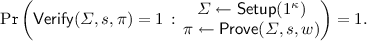
• 1. Completeness. For all $\kappa \in \mathbb {N}$, $(s, w) \in R$,

  

• 2. Computational soundness. For all PPT adversaries $\mathcal {A}$, the following probability is negligible in $\kappa$:

  

• 3. Zero-knowledge. There exists a PPT simulator $(\mathcal {S}_1, \mathcal {S}_2)$ such that $\mathcal {S}_1$ outputs a simulated CRS $\varSigma$ and trapdoor $\tau$; $\mathcal {S}_2$ takes as input $\varSigma$, a statement s and $\tau$, and outputs a simulated proof $\pi$; and, for all PPT adversaries $(\mathcal {A}_1,\mathcal {A}_2)$, the following probability is negligible in $\kappa$:

  

Definition 2.2

(Non-interactive Zero-knowledge Argument of Knowledge). A NIZK argument of knowledge for a relation R is a NIZK argument for R with the following additional extractability property:

• Extraction. For any PPT adversary $\mathcal {A}$, random string $r \overset{R}{\leftarrow }\{0,1\}^{*}$, there exists a PPT algorithm $\mathsf {Ext}$ such that the following probability is negligible in $\kappa$:

  

Definition 2.3

(zero-knowledge Succinct Non-interactive ARgument of Knowledge (zk-SNARK)). A zk-SNARK for a relation R is a non-interactive zero-knowledge argument of knowledge for R with the following additional property:

• Succinctness. For any s and w, the length of the proof $\pi$ is given by $\vert \pi \vert = \mathsf {poly}(\kappa ) \cdot \mathsf {polylog} (\vert s \vert + \vert w \vert )$.

2.2 Sigma Protocols

Sigma protocols are two-party interactive protocols of a specific structure. Let P (the prover) and V (the verifier) be two parties with common input s and a private input w for P. In a Sigma protocol, P sends a message a, V replies with a random $\kappa$-bit string r, P then sends a message e, and V decides to accept or reject based on the transcript (a, r, e). If V accepts (outputs 1), then the transcript is called accepting.

Definition 2.4

(Sigma protocol [28]). An interactive protocol between a prover P and a verifier V is a $\varSigma$ protocol for a relation R if the following properties are satisfied:

• 1. It is a three move public coin protocol.

• 2. Completeness: If P and V follow the protocol then $\Pr [ \left\langle P (w), V \right\rangle (s) = 1] = 1$ whenever $(s, w) \in R$.

• 3. Special soundness: There exists a polynomial time algorithm called the extractor which when given s and two transcripts (a, r, e) and $(a,r',e')$ that are accepting for s, with $r \ne r'$, outputs $w'$ such that $(s,w') \in R$.

• 4. Special honest verifier zero knowledge: There exists a polynomial time simulator which on input s and a random r outputs a transcript (a, r, e) with the same probability distribution as that generated by an honest interaction between P and V on (common) input s.

Fiat-Shamir transform. A $\varSigma$ protocol can be efficiently compiled into a non-interactive zero-knowledge proof of knowledge (in the random oracle model) through the Fiat-Shamir transform [34]. Not only the transformation removes interaction from the protocol, but also makes it zero-knowledge against malicious verifiers. At a high level, the transform works by having the prover compute the verifier’s message by applying an appropriate hash function, modeled as a random oracle in the security proof, to the prover’s first message to obtain a random challenge.

OR composition of $\varSigma$-protocols. In Cramer et al. [26], the authors devise an OR composition technique for Sigma protocols. Essentially, a prover can efficiently show $\left( (x_0 \in \mathcal {L}) \vee (x_1 \in \mathcal {L}) \right)$ without revealing which $x_i$ is in the language. More generally, the OR transform can handle two different relations $R_0$ and $R_1$.

Theorem 2.5

(OR-composition [26]). If $\varPi _0$ is a $\varSigma$-protocol for $R_0$ and $\varPi _1$ a $\varSigma$-protocol for $R_1$, then there is a $\varSigma$-protocol $\varPi _{\mathsf {OR}}$ for the relation $R_{\mathsf {OR}}$ given by $\{ ((x_0,x_1),w): \left( (x_0,w) \in R_0 \right) \vee \left( (x_1,w) \in R_1 \right) \}$.

Pedersen commitment. Throughout the paper, we use algebraic commitment schemes that allow proving linear relationships among committed values. The Pedersen commitment scheme [58] is one such example which gives unconditional hiding and computational binding properties based on the hardness of computing discrete logarithm in a group $\mathcal {G}$, say of order q. Given two random generators $g, h \in \mathcal {G}$ such that $\log _g h$ is unknown, a value $x \in \mathbb {Z}_q$ is committed to by choosing r randomly from $\mathbb {Z}_q$, and computing $g^x h^r$. We write $\mathsf {Com}_q(x)$ to denote a Pedersen commitment to x in a group of order q.

Sigma protocols are known in literature to prove knowledge of a committed value, equality of two committed values, and so on, and these protocols can be combined in natural ways. In particular, linear relationships between Pedersen commitments can be shown through existing techniques [18, 19, 37, 60]. For example, one could show that $y = ax + b$ for some public values a and b, given $\mathsf {Com}_q(x)$ and $\mathsf {Com}_q(y)$.

We use $\mathsf {PK}\lbrace (x,y, \ldots ): statements \text { about }x,y, \ldots \rbrace$ to denote a proof of knowledge of $x, y, \ldots$ that satisfies statements [19]. Other values in statements are public.

2.3 SNARK Construction from QAP

The work of Gennaro et al. [39] showed how to encode computations as quadratic programs. They show how to convert any Boolean circuit into a Quadratic Span Program (QSP) and any arithmetic circuit into a Quadratic Arithmetic Program (QAP). In this work, we will only use the latter definition. Even though QSPs are designed for Boolean circuits, arithmetic split gates defined in Parno et al. [57] translate an arithmetic wire into binary output wires, and Boolean functions may be computed using arithmetic gates. Parno et al. also note that such an arithmetic embedding results in a smaller QAP compared to the QSP of the original Boolean circuit. In the rest of the paper, we assume that Boolean functions are computed by a QAP defined over an arithmetic field, and hence will only be concerned with QAP.

Definition 2.6

(Quadratic Arithmetic Program [39]). A quadratic arithmetic program (QAP) Q over a field $\mathbb {F}$ consists of three sets of polynomials $V = \{ v_k(x) : k \in \{0, \ldots , m \} \}, W = \{ w_k(x) : k \in \{0, \ldots , m \} \}, Y = \{ y_k(x) : k \in \{0, \ldots , m \} \}$ and a target polynomial t(x), all in $\mathbb {F}[X]$.

Let $f: \mathbb {F}^n \rightarrow \mathbb {F}^{n'}$ be a function with input variables labeled $1,\ldots ,n$ and output variables labeled $m-n'+1, \ldots , m$. A QAP Q is said to compute f if the following holds: $a_1, \ldots , a_n, a_{m-n'+1}, \ldots , a_m \in \mathbb {F}^{n+n'}$ is a valid assignment to the input and output variables of f (i.e., $f(a_1, \ldots , a_n ) = (a_{m-n'+1}, \ldots , a_m)$) iff there exist $(a_{n+1}, \cdots , a_{m-n'}) \in \mathbb {F}^{m-n-n'}$ such that t(x) divides p(x), where

$$ p(x) = \left( v_0(x) + \displaystyle \sum _{k=1}^{m} a_k v_k(x) \right) . \left( w_0(x) + \displaystyle \sum _{k=1}^{m} a_k w_k(x) \right) - \left( y_0(x) + \displaystyle \sum _{k=1}^{m} a_k y_k(x) \right) . $$

The size of the QAP Q is m, and degree is deg(t(x)).

The polynomials $v_k(x), w_k(x), y_k(x)$ have degree at most deg$(t(x))-1$, since they can be reduced modulo t(x) without affecting the divisibility check.

3 NIZK on Committed IO for Algebraic Statements

In this section, we design Sigma protocols for knowledge of inputs and outputs of algebraic statements where the inputs and outputs are committed to. In other words, we enable proof of knowledge of $x_i$ given commitments $\mathsf {Com}(x_i)$ to inputs and a commitment $\mathsf {Com}(\varPi g_i^{P_i(x_i)})$ to the output of an algebraic function where $g_i$s are public generators in an elliptic curve group and $P_i$s are public single-variable polynomials. An important ingredient in this is a proof of knowledge of double discrete log which we elaborate on next.

3.1 Proof of Knowledge of Double Discrete Logarithm

Our goal is to prove the equality of a committed value and the discrete logarithm of another committed value. When the commitments are in elliptic curve groups, the known techniques for double discrete logarithm proofs will not work [19, 54]. This is because a group element cannot be naturally interpreted as a field element, as can be done in integer groups. Towards this end, we first describe a protocol to prove that the sum of two elliptic curve points that are committed to, is another public point on the curve.

In this section, we consider the family of curves E given by

$$\begin{aligned} y^2 = x^3 + ax+b, \end{aligned}$$

(1)

where $a,b \in \mathbb {F}_t$, but the techniques we describe below would extend to other curve families like Edwards [31]. The curve sec256k1 used by Bitcoin has the form of Eq. 1 with $a=0, b=7$.

The point addition relation is defined by the point addition equation specific to the curve family. Let $P = (x_1,y_1), Q = (x_2, y_2), P, Q \in E(\mathbb {F}_t)$ for the family E above. For distinct P, Q, $P \ne -Q$, $(x_3, y_3) = P+Q$ is given by

$$\begin{aligned} x_3&= \left( \dfrac{y_2 - y_1}{x_2 - x_1} \right) ^{2} - x_1 - x_2, \end{aligned}$$

(2)

$$\begin{aligned} y_3&= \frac{y_2 - y_1}{x_2 - x_1} (x_1 - x_3) - y_1. \end{aligned}$$

(3)

We use $\mathsf {addFormula}(P,Q)$ to denote $(x_3, y_3)$ computed in this way. When $P = Q$, the operation is doubling of the point P, denoted by $\mathsf {doubleFormula}(P)$. In this case, $(x_3, y_3)$ is given by

$$\begin{aligned} x_3&= \left( \dfrac{3 x_1^2 + a}{2 y_1} \right) ^{2} - 2x_1, \end{aligned}$$

(4)

$$\begin{aligned} y_3&= \frac{3 x_1^2 + a}{2 y_1} (x_1 - x_3) - y_1. \end{aligned}$$

(5)

We could prove the above relations for committed $x_1,x_2, y_1, y_2$ using known Sigma protocol techniques. But since the point addition computation is over $\mathbb {F}_t$, the commitments to the coordinates have to be in a group of order t, which is not necessarily the same as p, the order of the group $E(\mathbb {F}_t)$. The Complex Multiplication (CM) method could be used to find elliptic curve groups of a specific order. However, it is quite inefficient for large orders and would make our protocols impractical. We avoid the CM method by proposing a protocol that does not need to find a group of a given order.

We rewrite the point addition formula (Eqs. 2 and 3) as

$$\begin{aligned} x_3 x_2^{2} + x_3 x_1^{2} + x_1^{3} + x_2^{3} + 2 y_1 y_2&= y_2^{2} + y_1^{2} + x_1^{2} x_2 + x_1 x_2^{2} + 2 x_1 x_2 x_3, \end{aligned}$$

(6)

$$\begin{aligned} x_2 y_3 + x_3 y_2 + x_2 y_1&= x_1 y_2 + x_3 y_1 + x_1 y_3. \end{aligned}$$

(7)

Let $L_x$ and $R_x$ denote the left-hand side and right-hand side respectively of Eq. 6, and $L_y$ and $R_y$ of Eq. 7. That is:

$$\begin{aligned} L_x(x_1,y_1,x_2, y_2 )&= x_3 x_2^{2} + x_3 x_1^{2} + x_1^{3} + x_2^{3} + 2 y_1 y_2, \\ R_x(x_1,y_1,x_2, y_2 )&= y_2^{2} + y_1^{2} + x_1^{2} x_2 + x_1 x_2^{2} + 2 x_1 x_2 x_3, \\ L_y(x_1,y_1,x_2, y_2 )&= x_2 y_3 + x_3 y_2 + x_2 y_1, \\ R_y(x_1,y_1,x_2, y_2 )&= x_1 y_2 + x_3 y_1 + x_1 y_3. \end{aligned}$$

We use Sigma protocols to prove that $L_x, R_x, L_y$ and $R_y$ satisfy the above relations using committed intermediate values. To do so, in addition to linear relationships, our protocol needs to prove that a committed value is the product of two committed values: given $C_1 = \mathsf {Com}(a) = g^a h^{r_1}, C_2 = \mathsf {Com}(b) = g^b h^{r_2}, C_3 = \mathsf {Com}(c) = g^c h^{r_3}$, prove $c=ab$. This can be done by proving knowledge of b such that the discrete logarithm of $C_4$ with respect to $C_1$ is equal to the committed value in $C_2$, and the equality of committed values in $C_4$ and $C_3$, where $C_4 = C_1^b$. The prover computes and sends $C_4 = C_1^b$ with the following proof: $\mathsf {PK}\{ (a,b,c,b',c',r_1,r_2,r_3,r_4 ): C_1 = g^a h^{r_1} \wedge C_2 = g^b h^{r_2} \wedge C_3 = g^c h^{r_3} \wedge C_4 = C_1^{b'} \wedge C_4 = g^{c'} h^{r_4} \wedge b'=b \wedge c'=c \}$. In general, Sigma protocols for polynomial relationships among committed values were given by Camenisch and Michels [18].

Let $G_2$ be an elliptic-curve group of order q such that $q > 2 t^3$, and $P', Q'$ be points in $G_2$. We commit to the coordinates and the intermediate values necessary for the proof in $G_2$, and since the largest intermediate value in Eqs. 6 and 7 is cubic, the choice of q ensures there is no wrap around when the computation is modulo q. Since all computation on committed values will now be modulo q, and the addition equations are to be computed modulo t, we use division with remainder. We prove equality of $L_x$ and $R_x$ modulo q, divide them by t taking away multiples of t, and prove that the remainders are equal. When used together with appropriate range proofs to prove that the remainder does not exceed the divisor, and that the committed coordinates are in the desired range, we get equality modulo t. (There are several known techniques to build range proofs [14, 16], that is, to prove that $x \in [0,S]$ for a public S and committed x, including the recent, very efficient technique called Bulletproof [15].)

The protocol $\mathsf {addition}$ given in Fig. 1 proves that the addition formula holds for committed points P, Q and their sum T. We show that $\mathsf {addition}$ is secure in the full version. The protocol’s cost is dominated by the range proofs in steps 4, 5, 6 and the proof for polynomial relationships in steps 2 and 3. $\mathsf {addition}$ roughly has a proof size of $75+\log \log t$ elements, and prover’s work $60+\log t$ exponentiations.

Fig. 1.

$\mathsf {addition}:\mathsf {PK}\lbrace \left( P = (P_x,P_y), Q=(Q_x, Q_y) \right) : T = (T_x, T_y) = \mathsf {addFormula}(P,Q) \wedge \mathsf {C}_1 = \mathsf {Com}_{q}(P_x) \wedge \mathsf {C}_2 = \mathsf {Com}_{q}(P_y) \wedge \mathsf {C}_3 = \mathsf {Com}_{q}(Q_x) \wedge \mathsf {C}_4 = \mathsf {Com}_{q}(Q_y) \rbrace$

Let $\mathsf {C}_P = \mathsf {Com}_q(P) = (\mathsf {Com}_q(P_x),\mathsf {Com}_q(P_y))$ denote a commitment to a point $P=(P_x,P_y)$.

Theorem 3.1

Let $E(\mathbb {F}_t)$ be an elliptic curve given by Eq. 1, $T \in E$ and $q > 2t^3$. Then, $\mathsf {addition}$ in Fig. 1 is a $\varSigma$-protocol for the relation $R = \{((T, \mathsf {C}_P, \mathsf {C}_Q), (P, Q)): \mathsf {C}_P = \mathsf {Com}_q(P) \wedge \mathsf {C}_Q = \mathsf {Com}_q(Q) \wedge T = \mathsf {addFormula}(P,Q) \wedge P,Q \in E\}$.

Using techniques similar to the above protocol $\mathsf {addition}$, we obtain a protocol $\mathsf {double}$ to prove that doubling formula holds, i.e. $T=\mathsf {doubleFormula}(P)$. Now, we can handle all cases of point addition through the following statement:

This statement can be proved using OR composition of Sigma protocols: protocol $\mathsf {addition}$ for the first part of the OR statement, protocol $\mathsf {double}$ for the second, and simple Sigma protocols for the last component. We denote the proof of point addition of two committed points by $\mathsf {pointAddition}$.

For curves with a complete formula like Edwards, a point addition proof will not have different cases based on the relationship between P and Q.

Theorem 3.2

Let $E(\mathbb {F}_t)$ be an elliptic curve given by Eq. 1, $T \in E$ and $q > 2t^3$. Then, $\mathsf {pointAddition}$ is a $\varSigma$-protocol for the relation $R = \{ ((T, \mathsf {C}_P, \mathsf {C}_Q),$ $(P, Q)) : \mathsf {C}_P = \mathsf {Com}_q(P) \wedge \mathsf {C}_Q = \mathsf {Com}_q(Q) \wedge T = P+Q \wedge P,Q \in E\}$.

We note that the protocol $\mathsf {addition}$ may be modified to prove point addition for a committed point T in the following way. The proofs $\pi _1$ and $\pi _2$ are on committed coordinates $(T_x,T_y)$, and the range proof $\pi _3$ also includes proving the range of coordinates of T. We denote the point addition proof $\mathsf {PK}\lbrace \left( P, Q, T\right) : C_P = \mathsf {Com}_q(P) \wedge C_Q = \mathsf {Com}_q(Q) \wedge C_T = \mathsf {Com}_q(T) \wedge T = P + Q \wedge P, Q, T \in E \rbrace$ on all committed inputs by $\mathsf {comPointAddition}$.

We now construct a protocol to prove the equality of a committed value and the discrete logarithm of another committed value using the point addition proof. The double discrete logarithm proof is given in Fig. 2. (See the full version for a proof of security.) While the prover’s work is dominated by the protocol $\mathsf {pointAddition}$, we note that the range proofs for each challenge bit may be batched [15]. For soundness $2^{-60}$, the protocol $\mathsf {ddlog}$ incurs proof size of about $2370 + \log \log t$ elements and prover’s work of $1800+30 \log t$ exponentiations.

Fig. 2.

$\mathsf {ddlog}:\mathsf {PK}\lbrace (\lambda , x, y, r, r_1, r_2): \mathsf {Com}_{p}(\lambda ) = \lambda P + rQ \wedge \mathsf {Com}_{q}(x) = xP' + r_1 Q' \wedge \mathsf {Com}_{q}(y) = yP' + r_2Q' \wedge (x,y) = \lambda P \rbrace$

Theorem 3.3

Let $E(\mathbb {F}_t)$ be an elliptic curve given by Eq. 1, and $P \in E$ be an element of prime order p. Then, $\mathsf {ddlog}$ is a $\varSigma$-protocol for the relation $R = \{ (P, \mathsf {C}, \mathsf {C}_h,(\lambda , h)) : \mathsf {C} = \mathsf {Com}(\lambda ) \wedge \mathsf {C}_h = \mathsf {Com}(h) \wedge h = \lambda P, 0< \lambda < p \}$ with soundness 1/2.

3.2 Sigma Protocols on Committed Outputs

In this section, we construct Sigma protocols for committed output. First, we note a simpler construction when the output is a single bit. (This simpler variant is used in our OR compositions.) In particular, given an algebraic commitment to private input x, public y and an efficient Sigma protocol to prove that $f(x, y) = 1$, we show how to construct an efficient Sigma protocol to prove $f(x, y) = b$, for a committed bit b. Let $f: \mathbb {Z}_{q}^{n+m} \rightarrow \{0,1\}$, and let C be a commitment to the input x. Let $f_{\mathsf {com}}$ be the relation, $f_{\mathsf {com}}= \{ (y, (x,b) ): ((x,y) \in \mathcal {L}_{f} \wedge b=1) \vee (b=0 ) \}$. The Sigma protocol for the relation $f_{\mathsf {com}}$ is given by the proof $\mathsf {PK}\lbrace (b, x): f(x, y) = b \wedge D_b = g^b h^{r_1} \wedge C = g^{x} h^{r} \rbrace$. Let $\mathcal {G}$ be a group of order q, g a generator of $\mathcal {G}$, and h a random element of $\mathcal {G}$ such that the discrete logarithm of h with respect to g is unknown to the prover. Let $\varPi$ be a $\varSigma$-protocol for the relation f. The $\varSigma$-protocol for $f_{\mathsf {com}}$ is shown in Fig. 3.

Fig. 3.

$\mathsf {comBitSigma}: \mathsf {PK}\lbrace (b, x): f(x, y) = b \wedge D_b = g^b h^{r_1} \wedge C = g^{x} h^{r} \rbrace$

Theorem 3.4

If $\varPi$ is a $\varSigma$-protocol for f, then $\mathsf {comBitSigma}$ is a $\varSigma$-protocol for $f_{\mathsf {com}}$.

To generalize the above to the case where output is a group element and not a single bit, we need one more building block.

Proof of Point Addition and Discrete Log on Committed Points. Suppose we want to prove that a committed point is the sum of two group elements. But the challenge is that the input group elements are secret and are committed to, hence the prover also needs to prove knowledge of discrete logarithms of the input points with respect to a public base. Specifically, our goal is to design a protocol to prove knowledge of discrete logarithms of two committed points such that their sum is another committed point which we do using $\mathsf {comPointAddition}$. Let E be an elliptic curve defined over $\mathbb {F}_t$, and let $P \in E$ be an element of prime order p. Let $q > 2 t^3$ be a prime. The protocol $\mathsf {comSum}: \mathsf {PK}\lbrace (\gamma ,\alpha ,\beta ,x_1,x_2): \gamma = \alpha + \beta \wedge \alpha = x_1 P \wedge \beta = x_2 P \rbrace$ for $0< x_1,x_2 < p$ is shown in Fig. 4.

Fig. 4.

$\mathsf {comSum}: \mathsf {PK}\lbrace (\gamma ,\alpha ,\beta ,x_1,x_2 ): \gamma = \alpha + \beta \wedge \alpha = x_1 P \wedge \beta = x_2 P \rbrace$

When Committed Output is a Group Element. In the following discussion, similar to before, for a group element $\alpha = (\alpha _x, \alpha _y)$, where $\alpha _x, \alpha _y$ are the two coordinates of the elliptic curve point, the commitment to the point is performed by committing to its two coordinates in the proper group, i.e. $\mathsf {Com}(\alpha ) = (\mathsf {Com}(\alpha _x), \mathsf {Com}(\alpha _y))$.

We observe that given the above-mentioned building blocks i.e. $\mathsf {ddlog}$ and $\mathsf {comSum}$, we can construct Sigma protocol on a committed output group element for algebraic statements of the form $f(x_1, \ldots , x_n) = \varPi g_i^{P_i(x_i)}$. We sketch the ideas at a high-level for some simple functions. Let $f: \mathbb {Z} _p^{n} \rightarrow \mathcal {G}$, where $\mathcal {G}$ is a group $E(\mathbb {F}_t)$ of order p. When $f(x) = g^{x}$, then this reduces to the $\mathsf {ddlog}$ proof. For $f(x_1,x_2) = g_1^{x_1} g_2^{x_2}$, it suffices to commit to $g_1^{x_1}$ and $g_2^{x_2}$ separately and call the $\mathsf {comSum}$ proof. To consider higher degree polynomials in the exponent let us consider $f(x) = g^{x^2}$. To construct a proof $\mathsf {PK}\lbrace (x,y): g^{x^2} = y \wedge \mathsf {C}_1 = \mathsf {Com}(x) \wedge \mathsf {C}_2 = \mathsf {Com}(y) \rbrace$, the prover computes the commitments $C_1 = \mathsf {Com}_p(x)$, $C_2 = \mathsf {Com}_p(x^2)$ and $C_3 = \mathsf {Com}_q(k) = (\mathsf {Com}_q(k_x), \mathsf {Com}_q(k_y) )$, where $k = g^{x^2} = (k_x,k_y)$, for the choice of q as discussed in Sect. 3.1. Now, the prover gives the following proofs. $\mathsf {PK}\lbrace (x_2,k): k = g^{x_2} \wedge C_2 = \mathsf {Com}_p(x_2) \wedge C_3 = \mathsf {Com}_q(k) \rbrace$ using $\mathsf {ddlog}$, and a Sigma protocol for $\mathsf {PK}\lbrace (x_1,x_2): x_2 = x_1^2 \wedge C_1 = \mathsf {Com}_p(x_1) \wedge C_2 = \mathsf {Com}_p(x_2) \rbrace$. Given the above building blocks, it is easy to see that we can extend the techniques to devise proofs $\mathsf {comSigma}$ for $f(x_1, \ldots x_n) = \varPi g_i^{P_i(x_i)}$ .

4 NIZK on Committed IO for Non-Algebraic Statements

In this section we instantiate the following two building blocks which are critical for our NIZKs for composite statements.

• zk-SNARK on committed input. Given an algebraic commitment $C = g^x h^r$, and a circuit f, a zk-SNARK proof that $f(x, z) = b$.

• zk-SNARK on committed input and output. Given algebraic commitments $C_1 = g^x h^r, C_2 = g^b h^r$, and a circuit f, a zk-SNARK proof that $f(x, z) = b$.

We first give a brief high-level description of our central ideas. Our starting point is a SNARK where the proof consists of multi-exponentiation that resembles a Pedersen commitment. We identify what part of the proof allows commitments to a private input (witness) and private output (for hiding intermediate values of a larger computation) by suitably separating the input/output wires so there are corresponding distinct proof elements in the SNARK. We then commit to the private input and output of the SNARK proof independently using Pedersen commitment, and show equality of the committed values and the values in the multi-exponentiation proof element. While this observation has been used in prior works in verifiable computation [24, 35], it has been in different contexts and for different purposes. We briefly discuss how our ideas relate to two such ideas.

In [24], the authors present a verifiable computation scheme called Geppetto where the prover can share state across proofs. They generalize QAPs to create MultiQAPs which allow one to commit to data, and use it in many proofs. But crucially, all the proofs are for statements still represented as circuits while we also utilize the commitment to switch to sigma protocol proofs.

In [35], certain proof elements of a SNARK act as “accumulated” value of inputs in the context of large data size. The multi-exponentiations computed by the verifier in [35] act as a hash on data and different computations may be performed (verifiably) on it. The verifier computes the hash, and the proof verification involves checking the proof is consistent with the hash along with checks that the computation was performed correctly on the data using only the hash that was computed. On the other hand, in our setting, the multi-exponentiation is part of the proof, and computed by the prover, whose consistency across proofs must be shown. Additionally, these proofs could be different sigma protocols proving a variety of algebraic relations among some subset of the input used in the SNARK. Though our idea of exploiting a proof element with a certain structure is similar to the above works, we use it towards a different end.

For concreteness, we describe our protocol using the verifiable computation protocol Pinocchio [57] as a starting point. But our techniques carry over to other SNARK constructions as well. The key property we need from a SNARK construction is that the proof contains a multi-exponentiation of the input/output. Given this, we separate the circuit wires and obtain in a non-blackbox way, commitments as part of the SNARK proof.

Before giving the description of the above building blocks, we introduce an important ingredient: a protocol for proving equality of the discrete logarithms $(a_1, \ldots , a_n)$ in $y= \prod _{i=1}^n G_i^{a_i}$ and individual algebraic commitments to them. Using the standard notation, we denote the protocol by $\mathsf {PK}\lbrace (a_1, \ldots , a_n, r_1, \ldots , r_n): y = \prod _{i=1}^{n}G_i^{a_i} \wedge C_1 = g^{a_1} h^{r_1} \wedge \cdots \wedge C_n = g^{a_n} h^{r_n} \rbrace$. We include the steps of the protocol in the full version.

4.1 zk-SNARK on Committed Inputs

Recall that at a high level, each polynomial of the quadratic program (Definition 2.6), say, $v_k(x) \in \mathbb {F}[x]$ is mapped to an element in a bilinear group, $g^{v_k(s)}$, where s is a secret value chosen during CRS generation. Given these group elements and the values $a_i$ on the circuit wires which are the coefficients of the quadratic program, the prover can compute “in the exponent” to obtain $g^{v(s)}$, where $v(s) = \sum a_i v_k(s)$. The verifier uses the bilinear map to verify that the divisibility check of the QAP holds. We assume the computations are over large fields, that is, the QAP is defined over $\mathbb {F}_p$ for a large p. The size of the field is exponential in the security parameter. We omit p in all further descriptions of the field.

Let $f: \mathbb {F}^{N} \rightarrow \mathbb {F}^{n'}$ be a function with input/output values from $\mathbb {F}$, computed by an arithmetic circuit C with input wires labeled $1,\ldots ,N$, output wires labeled $m-n'+1, \ldots , m$. Let $\mathcal {Q}$ be a QAP of size m and degree d corresponding to C. We separate the circuit wires I into private input, public input, intermediate values, and output wires. Let $I_{com} \subseteq \{1, \ldots , N\}$ be the set of indices corresponding to the private inputs $a_1, \ldots , a_n$, $I_{pub}$ the indices for the public input wires, and $I_{out}$ the indices for the public output. Then let $I_{mid} = \{1, \ldots , m\} \setminus (I_{pub} \cup I_{com} \cup I_{out})$ be the indices of the intermediate wires. This way there are separate CRS elements corresponding to the private input and public input allowing the prover to compute corresponding proof elements. The divisibility check can still proceed, and we include additional span checks for the new proof elements. Now, we bind the multi-exponentiation corresponding to the private input in the proof to the value committed to in a Pedersen commitment using the protocol $\mathsf {comEq}$. Let $C_i = g^{a_i} h^{r_i}$ be a Pedersen commitment to the ith input $a_i$. The construction $\mathsf {comInSnark}: \mathsf {PK}\lbrace (a_1, \ldots , a_n, r_1, \ldots , r_n): f(a_1, \ldots a_n, z_1, \ldots , z_{N-n}) = (b_1, \ldots , b_{n'}) \wedge C_1 = g^{a_1} h^{r_1} \wedge \cdots \wedge C_n = g^{a_n} h^{r_n} \rbrace$ is given in Fig. 5.

Fig. 5.

$\mathsf {comInSnark}: \mathsf {PK}\lbrace (a_1, \ldots , a_n, r_1, \ldots , r_n): f(a_1, \ldots a_n, z_1, \ldots , z_{N-n}) = (b_1, \ldots , b_{n'}) \wedge C_1 = g^{a_1} h^{r_1} \wedge \ldots \wedge C_n = g^{a_n} h^{r_n} \rbrace$

Zero-knowledge. We make our construction zero-knowledge, and obtain zk$\mathsf {comInSnark}$, by randomizing the elements in the proof $\pi$ such that the checks verify and the proof is statistically indistinguishable from random group elements. Specifically, the prover chooses random $\delta _{v}, \delta _{w}, \delta _{y} \leftarrow \mathbb {F}$, and adds $\delta _{v} t(s)$ in the exponent to $v_{com}(s)$, $v_{mid}(s)$; $\delta _{w} t(s)$ to $w_{com}(s)$, $w_{mid}(s)$; and $\delta _{y} t(s)$ to $y_{com}(s)$, $y_{mid}(s)$. It is easy to see that the modified value of p(x) remains divisible by t(x). The following terms are added to $\mathsf {crs}$: $g_v^{t(s)}$, $\tilde{g}_w^{t(s)}$, $g_y^{t(s)}$, $g_v^{\alpha _v t(s)}$, $g_w^{\alpha _w t(s)}$, $g_y^{\alpha _y t(s)}$, $g_v^{\beta t(s)}$, $g_w^{\beta t(s)}$, $g_y^{\beta t(s)}$ ($g_v^{t(s)}$ is also added to $\mathsf {shortcrs}$). Prover can now compute the new values in $\pi$ from $\mathsf {crs}$, and they are verified in the same manner as before. The proof $\pi _{in}$ now proves a slightly different statement: $\mathsf {PK}\lbrace (a_1, \ldots , a_n, \delta , r_1, \ldots , r_n): y = H^{\delta } \prod _{i=1}^{n}G_i^{a_i} \wedge C_1 = g^{a_1} h^{r_1} \wedge \ldots \wedge C_n = g^{a_n} h^{r_n} \rbrace$. To verify it, the verifier uses $g_v^{t(s)}$ from $\mathsf {shortcrs}$.

Theorem 4.1

If q-PDH, 2q-SDH and d-PKE assumptions hold for $\mathsf {GroupGen}$ for $q \ge 4d+4$, then zk-$\mathsf {comInSnark}$ instantiated with a QAP of degree d is secure under Definition 2.2.

A proof of Theorem 4.1 can be found in the full version. Similarly, by separating the circuit wires into private input, public input, intermediate values and private output, we obtain zk-SNARK on committed input and output. We state the theorem below.

Theorem 4.2

If q-PDH, 2q-SDH and d-PKE assumptions hold for $\mathsf {GroupGen}$ for $q \ge 4d+4$, and discrete logarithm assumption holds in $\mathbb {G}$, then zk-$\mathsf {comIOSnark}$ instantiated with a QAP of degree d is secure under Definition 2.2.

5 Constructions for Compound Statements

In this section we use the building blocks we constructed in Sects. 4 and 3, to devise proofs for compound statements. In the following, we distinguish between functions that have an efficient algebraic representation versus functions that are efficiently represented as an arithmetic circuit over a field. Of course, any algebraic function can be written as a circuit over some field. But certain functions, modular exponentiation for instance, have a large circuit size and hence it is more desirable to not use a circuit in computing them. Therefore, when we say algebraic or arithmetic for functions below, we really mean the efficient representation of the function for computation. We say a function f is $\mathsf {arithmetic}$ if an arithmetic circuit is used to compute f, and say f is $\mathsf {algebraic}$ if it is represented algebraically. In this section, we show how to prove compound statements involving function compositions, OR, and AND. In our compositions, the SNARK used for the circuit could use a group whose order does not match with the group of the sigma protocol for the algebraic part. We construct a building block $\mathsf {Eq}$ to prove equality of committed values in different groups, given in the full version, which we use in our compositions.

5.1 Function Composition

We assume that the commitments we use in the following are in groups of correct order for the computation, so as to focus on the ideas for the composition. Wlog., our compositions hold even when the scalar field of the elliptic curve group, the field the curve is defined over and the field of the arithmetic circuit are all different, since we can prove equality of committed values in different groups using the protocol $\mathsf {Eq}$. We present the interactive variant for ease of presentation but note that all our constructions can be made non-interactive by running all the proofs in parallel and invoking the standard Fiat-Shamir transform (see Sect. 2.1). The constructions below also easily generalize to functions that have more input/output elements than shown, i.e. we can obtain constructions for statements of the form $\mathsf {PK}\lbrace (x_1,\ldots , x_n, y_1, \ldots , y_m): f_1(x_1,\ldots ,x_n,f_2(y_1, \ldots , y_m)) = z\rbrace$ where $f_1$, $f_2$ may each be arithmetic or algebraic. We give constructions $\mathsf {composition}$ by elaborating on the four possible compositions next:

• 1. $f_1$ and $f_2$ are functions represented as arithmetic circuits. Let $f_1: \mathbb {F}_p^2 \rightarrow \mathbb {F}_p$, and $f_2: \mathbb {F}_p \rightarrow \mathbb {F}_p$, and we want to prove knowledge of secrets $x_1,x_2$ such that $f_1(x_1,f_2(x_2)) = z$ for a public z. An example is proof of knowledge of $x_1$ and $x_2$ such that $H(x_1 || H(x_2)) = z$ where H is a collision resistant hash function such as SHA256. Such a composition can help reduce the size of CRS by composing the same or a few SNARK systems multiple times to obtain more complex statements without an increase in CRS size.

  

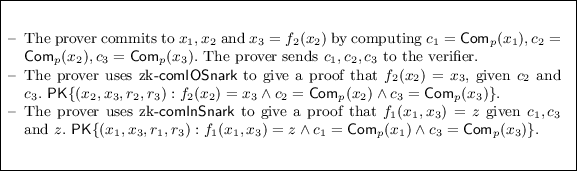
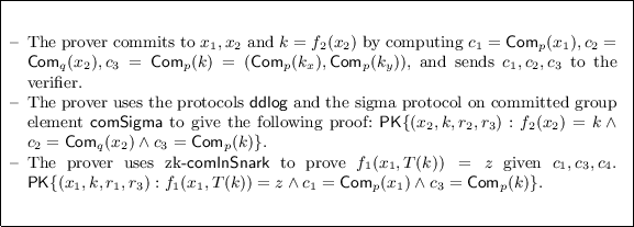
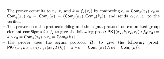
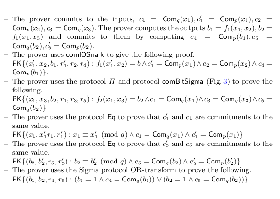
• 2. $f_1$ is an arithmetic circuit and $f_2$ is algebraic. Let $f_1: \mathbb {F} _p^{3} \rightarrow \mathbb {F} _p, f_2: \mathbb {Z} _q \rightarrow \mathcal {G}$ and $T: \mathcal {G} \rightarrow \mathbb {F} _p^{2}$. In this proof, we assume the algebraic function is over an elliptic curve group and assume the natural transformation for mapping an elliptic curve point to a tuple of field elements, i.e. its coordinates. Let $\mathcal {G}$ be an elliptic curve group of prime order q, and let $T(k) = (k_x, k_y)$ for $k \in \mathcal {G}$, where $(k_x, k_y)$ are the coordinates of the elliptic curve point. The following is a protocol for $\mathsf {PK}\lbrace (x_1, x_2): f_1 (x_1, T (f_2 (x_2))) = z \rbrace$. An example is proving knowledge of x such that $H(g^x) = z$.

  

• 3. $f_1$ is algebraic, and $f_2$ is an arithmetic circuit. Let $f_1: \mathbb {Z} _q^2 \rightarrow \mathcal {G}, f_2: \mathbb {F} _p \rightarrow \mathbb {F} _p$. Let $\varPi$ be a $\varSigma$-protocol for $f_1$. The following is a protocol for $\mathsf {PK}\lbrace (x_1, x_2): f_1 (x_1, f_2 (x_2)) = z \rbrace$. An example is proving knowledge of x such that $g^{H(x)} = z$ where H is a hash function. This composition commonly appears when proving knowledge of a digitally signed message.

  

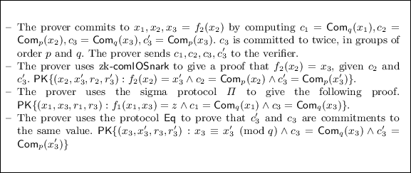
• 4. $f_1$ and $f_2$ are algebraic. Let $f_1: \mathbb {Z} _p^3 \rightarrow \mathcal {G} _1, f_2: \mathbb {Z} _q \rightarrow \mathcal {G} _2$, where $\mathcal {G} _1$ and $\mathcal {G} _2$ are elliptic curve groups of prime order p and q respectively. Let $T(k) = (k_x, k_y)$ for $k \in \mathcal {G} _2$, where $(k_x, k_y)$ are the coordinates of the elliptic curve point. Let $\varPi _1$ be a $\varSigma$-protocol for $f_1$. Let $x_1 \in \mathbb {Z} _p, x_2 \in \mathbb {Z} _q$. An example is proving knowledge of x such that $g_1^{T(g_2^x)}$ for generators $g_1$ and $g_2$ for two different groups and a valid transformation T for mapping from one group to another. These statements often occur in anonymous credential constructions or proving statements about accumulators but the only previous constructions are for RSA groups.

  

Theorem 5.1

(Function Composition). The constructions $\mathsf {composition}$ are non-interactive zero-knowledge arguments $\mathsf {PK}\lbrace (x_1,\ldots , x_n, y_1, \ldots , y_m): f_1(x_1,\ldots , x_n, f_2(y_1, \ldots , y_m)) = z\rbrace$, as per Definition 2.2, for any $f_1, f_2 \in \{ \mathsf {algebraic}, \mathsf {arithmetic} \}$ assuming the security of zk-$\mathsf {comInSnark}$, zk-$\mathsf {comIOSnark}$, $\mathsf {ddlog}$, $\mathsf {Eq}$.

5.2 OR Composition

Consider the OR composition where a prover wants to show that $f_1 (x_1, x_2) = 1$ or $f_2(x_1,x_3) = 1$ but without revealing which one is true. We give constructions $\mathsf {compoundOR}: \mathsf {PK}\lbrace (x_1, x_2, x_3): f_1 (x_1, x_2) \vee f_2(x_1,x_3) = 1 \rbrace$, where the $f_i$s could have either an arithmetic or algebraic representation, and could have shared secret inputs.

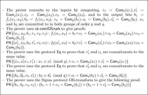
• 1. $f_1$ and $f_2$ are functions represented as arithmetic circuits. Let $f_1: \mathbb {F}_p^2 \rightarrow \{0,1\}$, and $f_2: \mathbb {F}_q^2 \rightarrow \{0,1\}$, $q<p$. An example is composing proofs for two SNARK systems that work over different elliptic curve groups.

  

• 2. One of them is an arithmetic circuit and the other is an algebraic relation. Wlog., $f_1$ is represented as an arithmetic circuit and $f_2$ is an algebraic statement. Let $f_1: \mathbb {F} _p^{2} \rightarrow \{0,1\}, f_2: \mathbb {Z} _q^{2} \rightarrow \{0,1\}, q < p$. Let $\varPi$ be a $\varSigma$-protocol for $f_2$. An example is proving knowledge of x such that $H(x) = y$ OR $g^x = z$.

  

Let $f_{\mathsf {OR}}$ be the relation given by $f_{\mathsf {OR}} = \{ ((f_1, f_2), (x_1,x_2, x_3)): \left( (x_1,x_2) \in R_{f_1} \right)$ $\vee \left( (x_1, x_3) \in R_{f_2} \right) \}$.

Theorem 5.2

(OR Composition). The constructions $\mathsf {compoundOR}$ are non-interactive zero-knowledge arguments $\mathsf {PK}\lbrace (x_1, x_2, x_3): f_1 (x_1, x_2) \vee f_2(x_1,x_3) = 1 \rbrace$, as per Definition 2.2, for the relation $f_{\mathsf {OR}}$, for any $f_1, f_2 \in \{ \mathsf {algebraic}, \mathsf {arithmetic} \}$, assuming the security of zk-$\mathsf {comInSnark}$, zk-$\mathsf {comIOSnark}$, $\mathsf {comBitSigma}$, $\mathsf {Eq}$.

5.3 AND Composition

Techniques shown in Sect. 5.2 extend for proofs of the form, $\mathsf {PK}\lbrace (x_1, x_2, x_3): f_1 (x_1, x_2) \wedge f_2(x_1,x_3) = 1 \rbrace$ for all combinations of $f_1$ and $f_2$ being arithmetic and algebraic. In particular, to prove the AND of multiple statements, we use our building blocks $\mathsf {comInSnark}$ for the arithmetic part, $\varSigma$-protocol for the algebraic part, and $\mathsf {Eq}$ to switch between groups.

6 Applications

6.1 Privacy-preserving Audits of Bitcoin Exchanges

In this section, we show how to use our constructions for proving composite statements in zero-knowledge to build a privacy-preserving proof of solvency for Bitcoin exchanges. A proof of solvency demonstrates that an exchange controls sufficient reserves to settle each customer’s account. If the exchange loses a large amount of money in an attack, it would not be able to provide such a proof. Thus customers will find out about the attack very soon and take necessary actions.

A proof of solvency consists of three components:

• A proof of liabilities that allows customers to verify that their accounts are included in the total.

• A proof of assets which shows that the exchange has a certain amount of reserves.

• A proof that the reserves cover the liabilities to an acceptable degree.

Let g, h be fixed public generators of a group G of order q. For a Bitcoin public key y, $x \in \mathbb {Z}_q$ is the corresponding secret key such that $y = g^{x}$. In the proof of assets below, for a group element $k=(k_x,k_y)$, we write $\mathsf {Com}(k)$ to mean a commitment to the coordinates of k, i.e. $\mathsf {Com}(k) = (\mathsf {Com}(k_x),\mathsf {Com}(k_y))$. The Bitcoin address corresponding to a key y is given by $\mathsf {h} = H(y)$, where H hashes y to a more compact representation. We denote the balance associated with an address $\mathsf {h}$ by $\mathsf {bal}(\mathsf {h})$.

Proof of assets. We give the proof of assets in Fig. 6, which allows an exchange to generate a commitment to its total assets along with a zero-knowledge proof that the exchange knows the private keys for a set of Bitcoin addresses whose total value is equal to the committed value. The exchange creates a set of hashes $\mathcal {PK}$ to serve as an anonymity set: $\mathcal {PK} = \{ \mathsf {h}_1, \cdots , \mathsf {h}_n \}$ from the public data available on the blockchain. Let $x_1, \cdots , x_n$ be the corresponding secret keys, so that $\mathsf {h}_i = H(g^{x_i})$, $s_i$ indicates whether the exchange knows the ith secret key. The total assets can now be expressed as $\mathsf {Assets} = \sum _{i=1}^{n} s_i \cdot \mathsf {bal}(\mathsf {h}_i)$. The public data available on the blockchain is $\mathsf {h}_i = H(y_i), p_i = g^{\mathsf {bal}(\mathsf {h}_i)}$ for all $i \in [1, n]$.

Fig. 6.

Proof of assets

Zero-knowledge and soundness of the proof of assets follow from properties of our constructions for compound statements (Theorems 5.1 and 5.2) and properties of the Sigma protocols used. Proofs of liabilities and solvency have been moved to the full version because they are very similar to Provisions. We compare the trade-off between proof size and prover’s work in our approach versus Provisions and a full SNARK solution in Table 1 in Appendix A.

6.2 Privacy-Preserving Credentials

Another application of our compositions for compound statements is in privacy-preserving verification of credentials. A credential system allows a user to obtain credentials from an organization or a Certificate Authority, and later prove to a verifier that she has been given appropriate credentials. Typically, the user’s credentials will contain a set of attributes, and the verifier will require that the user prove that the attributes in his credential satisfy certain policy. Many different constructions have been proposed for anonymous credential systems built around sigma protocols. The signatures used, therefore, are specially designed so that a sigma protocol can be used to prove knowledge of the signature on a committed message. If we want to base anonymous credentials on standard signatures, like RSA signatures, we will need to prove a compound statement involving an algebraic relation (for the exponentiation), and a circuit-based statement (for the hash function). The recent work of [30] achieves privacy-preserving verification of X.509 certificates by using zk-SNARKs, and this involves representing the exponentiation in an RSA group as a circuit. Here, we use our composition constructions to build an efficient proof avoiding expensive circuit representation of algebraic statements.

Given a SHA hash digest of a message m, a candidate RSA signature $\sigma$, and an RSA modulus N, verification involves checking whether $\sigma ^{e} \mod n = h$, where $h = \mathsf {padding}(\mathsf {SHA}(m))$. The construction given in Fig. 7 achieves privacy-preserving verification for credentials based on RSA signatures. We compare the trade off between the proof size and prover’s work in our approach versus other methods in Table 2 in Appendix A. Our compositions and similar techniques extend to yield efficient privacy-preserving verification for credentials based on existing infrastructure like standard RSA-PSS, RSA-PKCS etc.

Fig. 7.

RSA signature verification

A Efficiency

We briefly discuss the estimated cost of some of the building blocks. The $\mathsf {ddlog}$ proof is dominated by the cost of the range proofs in steps 4, 5, 6 of $\mathsf {pointAddition}$ protocol in Fig. 1. In a recent work [15], it was shown how to prove that a committed value is in a range using only a number of field elements that is logarithmic in the bit length of the range. Using these proofs to instantiate all the necessary range proofs in protocol $\mathsf {pointAddition}$, the prover’s work is $30 \log t+1800$ group exponentiations, the verifier’s work is $10 \log t$ exponentiations, and the proof size is $2370+ \log \log t$ elements where the proof is for a curve defined over $\mathbb {F}_t$. The cost of $\mathsf {comInSnark}$ is the cost of the $\mathsf {comEq}$ in addition to the cost incurred by separating the wires in the underlying SNARK construction. The proof size of $\mathsf {comInSnark}$ is 15 group elements, and 2 field elements for every committed value (input/output). In the case of our following applications, the proof size is 17 elements. The prover’s work is the number of exponentiations for computing the SNARK proof and an additional 2 exponentiations for the $\mathsf {comEq}$ proof. The verifier’s work is 2 exponentiations and 21 pairings. Similarly, $\mathsf {comIOSnark}$ has proof size 26 elements, the prover’s work, in addition to the exponentiations for the SNARK proof is 4 exponentiations and the verifier’s work is 4 exponentiations and 30 pairings.

Proof of solvency. In Table 1, we compare the proof size and prover’s work of Provisions with our protocol and a solution that uses zk-SNARK for the entire statement. The proof size and prover’s work are dominated by the range proofs; the numbers below give only the dominating terms ignoring small constants and are assuming that the range proofs are realized using Bulletproofs.

Table 1. Comparison of prover work and proof sizes for proof of solvency using different methods. n is the size of the anonymity set, c is the number of customer accounts, m is $\lceil \log \mathsf {Max} \rceil = 51$, p is the bit length of the modulus for exponentiation (size of the field over which the curve is defined). For $n=500,000$ and $c = 2$ million, the proof size and prover’s work in Provisions is $5*10^{6}$ and $4*10^{7}$ respectively. For the same parameters, our approach gives proof size of $10^{9}$ and prover’s work $10^{10}$, while also achieving the additional pay-to-hash functionality. A fully zk-SNARK solution requires prover’s work roughly $10^{13}$. (Exp. stands for exponentiations.)

Privacy preserving credentials. In Table 2, we compare the proof size and prover’s work in privacy-preserving credentials for Cinderella, the interactive protocol of [21], and our composition.

Table 2. Comparison of prover work and proof sizes for credential verification using different methods. p is the order of the group in which commitments are computed, $\vert m \vert$ is the bit length of the message. For $e = 65537, \log p= 256, \vert H \vert =23785$, we note an 87% decrease in prover’s work compared to Cinderella at the cost of increasing the proof size to 298 from 7 group elements. (Exp. stands for exponentiations.)