Finer Resolution Mapping of Marine Aquaculture Areas Using WorldView-2 Imagery and a Hierarchical Cascade Convolutional Neural Network

 , ,
, ,
Abstract
:
1. Introduction
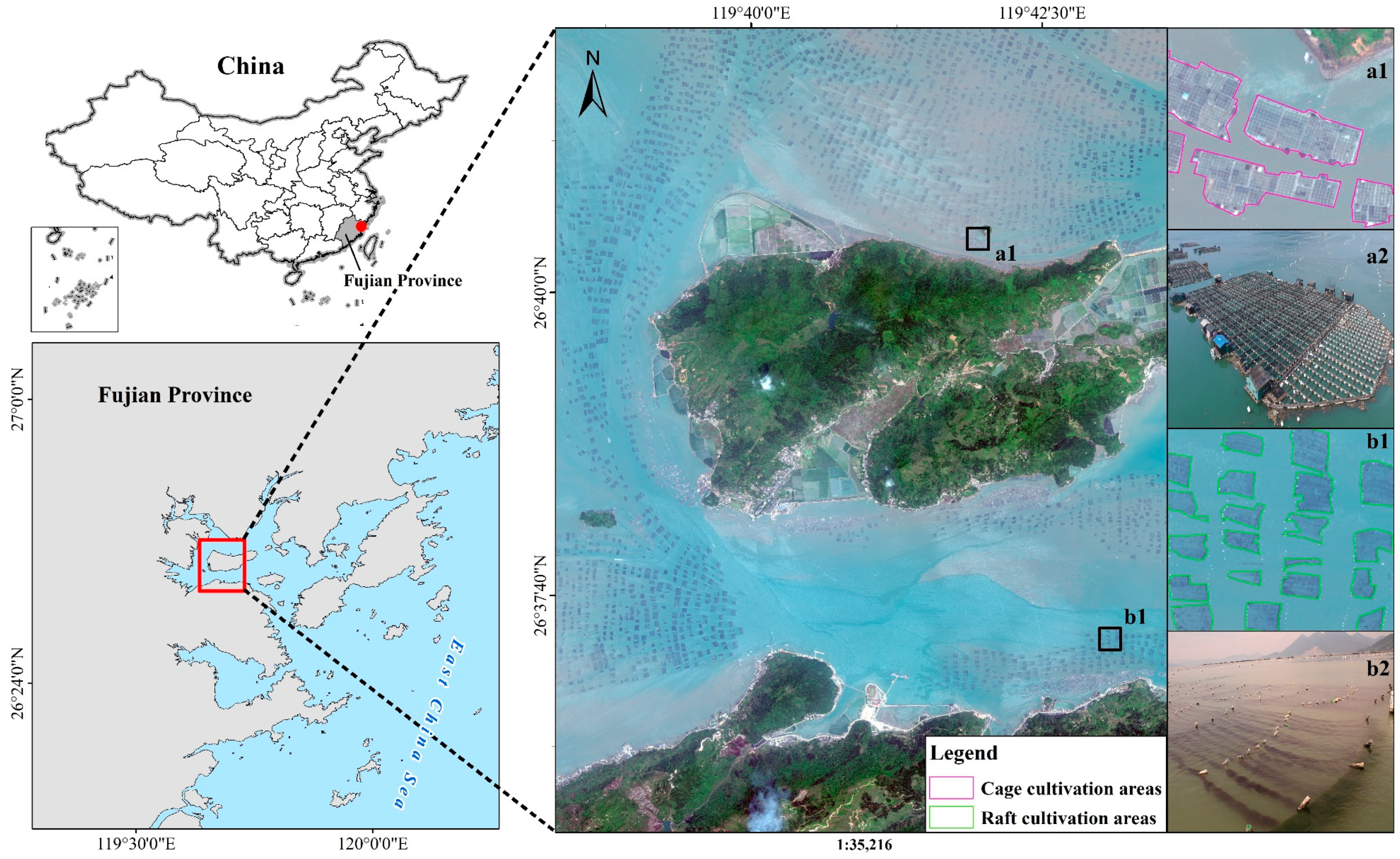
2. Study Area
3. Materials and Methods
3.1. Data and Preprocessing
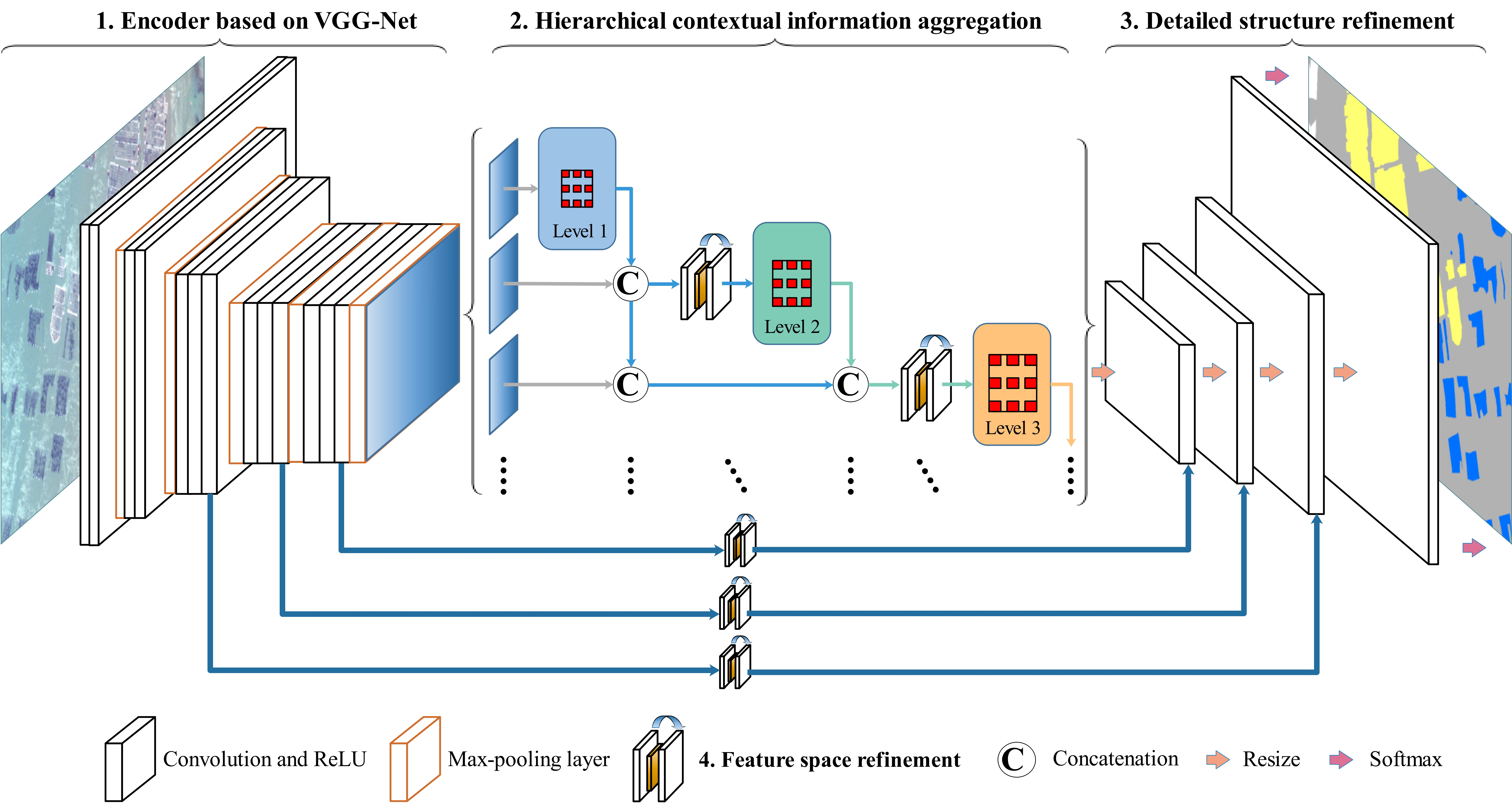
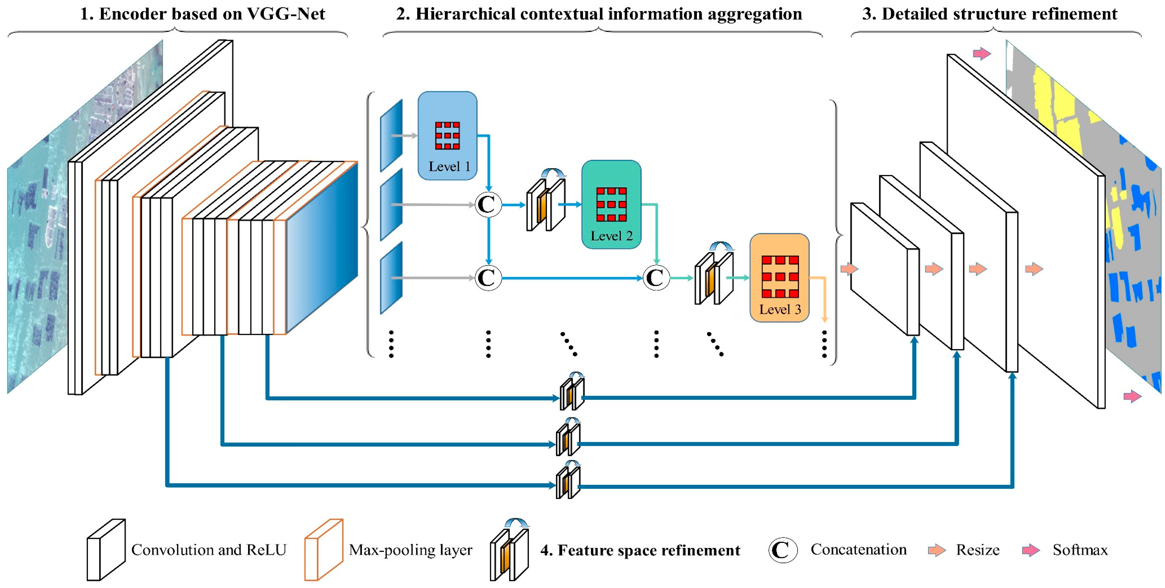
3.2. Hierarchical Convolutional Neural Network
3.2.1. Encoder Based on VGG-Net
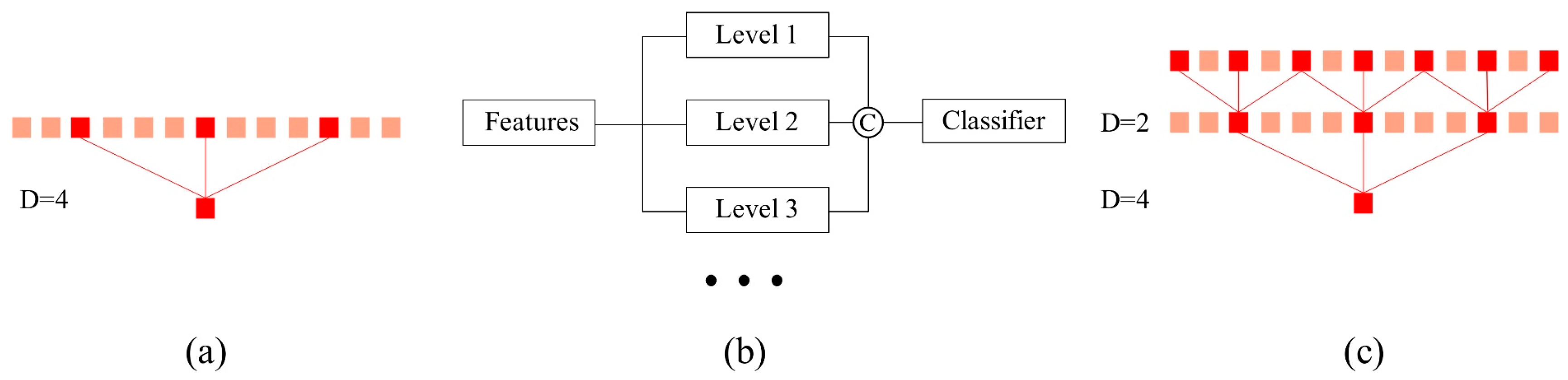
3.2.2. Hierarchical Contextual Information Aggregation
3.2.3. Detailed Structure Refinement
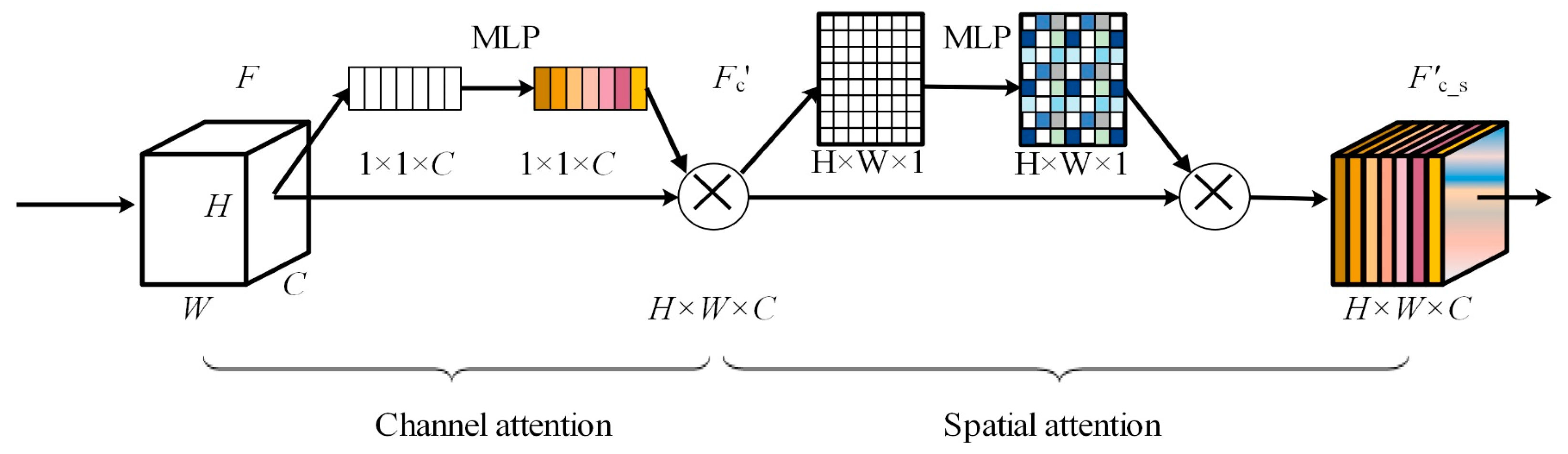
3.2.4. Feature Space Refinement
3.3. Implementation Details
3.4. Comparison Methods
3.4.1. Object-Based Support Vector Machine (SVM) Classification
3.4.2. FCN-Based Methods
3.5. Accuracy Assessment and Comparison
4. Results and Comparison
4.1. Classification Results and Accuracy Assessment
4.2. Accuracy Comparison
5. Discussion
5.1. OBIA vs. Our Approach
5.2. Conventional FCN-Based Methods vs. Our Approach
5.3. Ablation Analysis
5.4. Potential Applications and Limitations
6. Conclusions
Author Contributions
Funding
Acknowledgments
Conflicts of Interest
References
- Gentry, R.R.; Froehlich, H.E.; Grimm, D.; Kareiva, P.; Parke, M.; Rust, M.; Gaines, S.D.; Halpern, B.S. Mapping the global potential for marine aquaculture. Nat. Ecol. Evol. 2017, 1, 1317–1324. [Google Scholar] [CrossRef] [PubMed]
- Campbell, B.; Pauly, D. Mariculture: A global analysis of production trends since 1950. Mar. Policy 2013, 39, 94–100. [Google Scholar] [CrossRef]
- Burbridge, P.; Hendrick, V.; Roth, E.; Rosenthal, H. Rosenthal Social and economic policy issues relevant to marine aquaculture. J. Appl. Ichthyol. 2001, 17, 194–206. [Google Scholar] [CrossRef]
- FAO. The State of World Fisheries and Aquaculture; FAO: Rome, Italy, 2004; ISBN 9251051771. [Google Scholar]
- FAO. The State of World Fisheries and Aquaculture; FAO: Rome, Italy, 2018; ISBN 9789251305621. [Google Scholar]
- Grigorakis, K.; Rigos, G. Aquaculture effects on environmental and public welfare—The case of Mediterranean mariculture. Chemosphere 2011, 85, 899–919. [Google Scholar] [CrossRef] [PubMed]
- Cao, L.; Wang, W.; Yang, Y.; Yang, C.; Yuan, Z.; Xiong, S.; Diana, J. Environmental impact of aquaculture and countermeasures to aquaculture pollution in China. Environ. Sci. Pollut. Res. 2007, 14, 452–462. [Google Scholar]
- Tovar, A.; Moreno, C.; Mánuel-Vez, M.P.; García-Vargas, M. Environmental impacts of intensive aquaculture in marine waters. Water Res. 2000, 34, 334–342. [Google Scholar] [CrossRef]
- Lillesand, T.; Kiefer, R.W.; Chipman, J. Remote Sensing and Image Interpretation, 5th ed.; John Wiley & Sons: Hobokan, NJ, USA, 2004; ISBN 0471152277. [Google Scholar]
- Fan, J.; Chu, J.; Geng, J.; Zhang, F. Floating raft aquaculture information automatic extraction based on high resolution SAR images. In Proceedings of the 2015 IEEE International Geoscience and Remote Sensing Symposium (IGARSS), Milan, Italy, 26–31 July 2015; pp. 3898–3901. [Google Scholar]
- Lu, Y.; Li, Q.; Du, X.; Wang, H.; Liu, J. A Method of Coastal Aquaculture Area Automatic Extraction with High Spatial Resolution Images. Remote Sens. Technol. Appl. 2015, 30, 486–494. [Google Scholar] [CrossRef]
- Zheng, Y.; Wu, J.; Wang, A.; Chen, J. Object-and pixel-based classifications of macroalgae farming area with high spatial resolution imagery. Geocarto Int. 2017, 33, 1048–1063. [Google Scholar] [CrossRef]
- Fu, Y.; Deng, J.; Ye, Z.; Gan, M.; Wang, K.; Wu, J.; Yang, W.; Xiao, G. Coastal aquaculture mapping from very high spatial resolution imagery by combining object-based neighbor features. Sustainability 2019, 11, 637. [Google Scholar] [CrossRef]
- Wang, M.; Cui, Q.; Wang, J.; Ming, D.; Lv, G. Raft cultivation area extraction from high resolution remote sensing imagery by fusing multi-scale region-line primitive association features. ISPRS J. Photogramm. Remote Sens. 2017, 123, 104–113. [Google Scholar] [CrossRef]
- Shi, T.; Xu, Q.; Zou, Z.; Shi, Z. Automatic Raft Labeling for Remote Sensing Images via Dual-Scale Homogeneous Convolutional Neural Network. Remote Sens. 2018, 10, 1130. [Google Scholar] [CrossRef]
- Blaschke, T.; Hay, G.J.; Kelly, M.; Lang, S.; Hofmann, P.; Addink, E.; Queiroz Feitosa, R.; van der Meer, F.; van der Werff, H.; van Coillie, F.; et al. Geographic Object-Based Image Analysis—Towards a new paradigm. ISPRS J. Photogramm. Remote Sens. 2014, 87, 180–191. [Google Scholar] [CrossRef] [PubMed]
- Farabet, C.; Couprie, C.; Najman, L.; Lecun, Y. Learning hierarchical features for scene labeling. IEEE Trans. Pattern Anal. Mach. Intell. 2013, 35, 1915–1929. [Google Scholar] [CrossRef] [PubMed]
- LeCun, Y.; Bottou, L.; Bengio, Y.; Haffner, P. Gradient-based learning applied to document recognition. Proc. IEEE 1998, 86, 2278–2324. [Google Scholar] [CrossRef] [Green Version]
- Arel, I.; Rose, D.; Karnowski, T. Deep machine learning-A new frontier in artificial intelligence research. IEEE Comput. Intell. Mag. 2010, 5, 13–18. [Google Scholar] [CrossRef]
- Schmidhuber, J. Deep Learning in neural networks: An overview. Neural Netw. 2015, 61, 85–117. [Google Scholar] [CrossRef]
- Dong, Z.; Wu, Y.; Pei, M.; Jia, Y. Vehicle Type Classification Using a Semisupervised Convolutional Neural Network. IEEE Trans. Intell. Transp. Syst. 2015, 16, 2247–2256. [Google Scholar] [CrossRef]
- Hu, F.; Xia, G.S.; Hu, J.; Zhang, L. Transferring deep convolutional neural networks for the scene classification of high-resolution remote sensing imagery. Remote Sens. 2015, 7, 14680–14707. [Google Scholar] [CrossRef]
- Sharma, A.; Liu, X.; Yang, X.; Shi, D. A patch-based convolutional neural network for remote sensing image classification. Neural Netw. 2017, 95, 19–28. [Google Scholar] [CrossRef]
- Santara, A.; Mani, K.; Hatwar, P.; Singh, A.; Garg, A.; Padia, K.; Mitra, P. Bass net: Band-adaptive spectral-spatial feature learning neural network for hyperspectral image classification. IEEE Trans. Geosci. Remote Sens. 2017, 55, 5293–5301. [Google Scholar] [CrossRef]
- Lagrange, A.; Le Saux, B.; Beaupere, A.; Boulch, A.; Chan-Hon-Tong, A.; Herbin, S.; Randrianarivo, H.; Ferecatu, M. Benchmarking classification of earth-observation data: From learning explicit features to convolutional networks. In Proceedings of the International Geoscience and Remote Sensing Symposium (IGARSS), Milan, Italy, 26–31 July 2015; pp. 4173–4176. [Google Scholar]
- Maggiori, E.; Tarabalka, Y.; Charpiat, G.; Alliez, P. Convolutional Neural Networks for Large-Scale Remote-Sensing Image Classification. IEEE Trans. Geosci. Remote Sens. 2017, 55, 645–657. [Google Scholar] [CrossRef]
- Audebert, N.; Le Saux, B.; Lefèvre, S. How Useful is Region-based Classification of Remote Sensing Images in a Deep Learning Framework? In Proceedings of the 2016 IEEE International Geoscience and Remote Sensing Symposium (IGARSS), Beijing, China, 10–15 July 2016; pp. 5091–5094. [Google Scholar]
- Zhang, C.; Sargent, I.; Pan, X.; Li, H.; Gardiner, A.; Hare, J.; Atkinson, P.M. An object-based convolutional neural network (OCNN) for urban land use classification. Remote Sens. Environ. 2018, 216, 57–70. [Google Scholar] [CrossRef] [Green Version]
- Fu, Y.; Liu, K.; Shen, Z.; Deng, J.; Gan, M.; Liu, X.; Lu, D.; Wang, K. Mapping Impervious Surfaces in Town-Rural Transition Belts Using China’s GF-2 Imagery and Object-Based Deep CNNs. Remote Sens. 2019, 11, 280. [Google Scholar] [CrossRef]
- Long, J.; Shelhamer, E.; Darrell, T. Fully convolutional networks for semantic segmentation. In Proceedings of the IEEE Computer Society Conference on Computer Vision and Pattern Recognition, Boston, MA, USA, 7–12 June 2015; pp. 3431–3440. [Google Scholar]
- Eigen, D.; Fergus, R. Predicting depth, surface normals and semantic labels with a common multi-scale convolutional architecture. In Proceedings of the IEEE International Conference on Computer Vision (ICCV), Santiago, Chile, 7–13 December 2015; pp. 2650–2658. [Google Scholar]
- Zhao, W.; Du, S. Learning multiscale and deep representations for classifying remotely sensed imagery. ISPRS J. Photogramm. Remote Sens. 2016, 113, 155–165. [Google Scholar] [CrossRef]
- Liu, Y.; Zhong, Y.; Fei, F.; Zhang, L. Scene semantic classification based on random-scale stretched convolutional neural network for high-spatial resolution remote sensing imagery. In Proceedings of the 2016 IEEE International Geoscience and Remote Sensing Symposium (IGARSS), Beijing, China, 10–15 July 2016; pp. 763–766. [Google Scholar]
- Chen, L.-C.; Papandreou, G.; Kokkinos, I.; Murphy, K.; Yuille, A.L. DeepLab: Semantic Image Segmentation with Deep Convolutional Nets, Atrous Convolution, and Fully Connected CRFs. IEEE Trans. Pattern Anal. Mach. Intell. 2018, 40, 834–848. [Google Scholar] [CrossRef] [PubMed]
- He, K.; Zhang, X.; Ren, S.; Sun, J. Spatial Pyramid Pooling in Deep Convolutional Networks for Visual Recognition. IEEE Trans. Pattern Anal. Mach. Intell. 2015, 37, 1904–1916. [Google Scholar] [CrossRef] [PubMed] [Green Version]
- Zhao, H.; Shi, J.; Qi, X.; Wang, X.; Jia, J. Pyramid scene parsing network. In Proceedings of the 2017 IEEE Conference on Computer Vision and Pattern Recognition (CVPR), Honolulu, HI, USA, 21–26 July 2017; pp. 6230–6239. [Google Scholar]
- Audebert, N.; Le Saux, B.; Lefèvre, S. Semantic segmentation of earth observation data using multimodal and multi-scale deep networks. In Proceedings of the Asian Conference on Computer Vision (ACCV16), Taipei, Taiwan, 20–24 November 2016; pp. 180–196. [Google Scholar]
- Ronneberger, O.; Fischer, P.; Brox, T. U-Net: Convolutional Networks for Biomedical Image Segmentation. In Proceedings of the Medical Image Computing and Computer-Assisted Intervention (MICCAI 2015), Munich, Germany, 5–9 October 2015; pp. 234–241. [Google Scholar]
- Hariharan, B.; Arbeláez, P.; Girshick, R.; Malik, J. Hypercolumns for object segmentation and fine-grained localization. In Proceedings of the 2015 IEEE Conference on Computer Vision and Pattern Recognition (CVPR), Boston, MA, USA, 7–12 June 2015; pp. 447–456. [Google Scholar]
- Pinheiro, P.O.; Lin, T.Y.; Collobert, R.; Dollár, P. Learning to refine object segments. In Proceedings of the European Conference on Computer Vision, Amsterdam, The Netherlands, 8–16 October 2016; pp. 75–91. [Google Scholar]
- Noh, H.; Hong, S.; Han, B. Learning deconvolution network for semantic segmentation. In Proceedings of the IEEE International Conference on Computer Vision (ICCV), Santiago, Chile, 7–13 December 2015; pp. 1520–1528. [Google Scholar]
- Badrinarayanan, V.; Kendall, A.; Cipolla, R. SegNet: A Deep Convolutional Encoder-Decoder Architecture for Image Segmentation. IEEE Trans. Pattern Anal. Mach. Intell. 2017, 39, 2481–2495. [Google Scholar] [CrossRef] [PubMed]
- Bertasius, G.; Shi, J.; Torresani, L. Semantic Segmentation with Boundary Neural Fields. In Proceedings of the 2016 IEEE Conference on Computer Vision and Pattern Recognition (CVPR), Las Vegas, NV, USA, 26 June–1 July 2016; pp. 3602–3610. [Google Scholar]
- Marmanis, D.; Schindler, K.; Wegner, J.D.; Galliani, S.; Datcu, M.; Stilla, U. Classification with an edge: Improving semantic image segmentation with boundary detection. ISPRS J. Photogramm. Remote Sens. 2018, 135, 158–172. [Google Scholar] [CrossRef] [Green Version]
- Wolf, A. Using WorldView 2 Vis-NIR MSI Imagery to Support Land Mapping and Feature Extraction Using Normalized Difference Index Ratios. In Algorithms and Technologies for Multispectral, Hyperspectral, and Ultraspectral Imagery; SPIE: Baltimore, MD, USA, 2012; Volume 8390, p. 83900N. [Google Scholar]
- Lin, C.; Wu, C.C.; Tsogt, K.; Ouyang, Y.C.; Chang, C.I. Effects of atmospheric correction and pansharpening on LULC classification accuracy using WorldView-2 imagery. Inf. Process. Agric. 2015, 2, 25–36. [Google Scholar] [CrossRef] [Green Version]
- Karen, S.; Andrew, Z. Very Deep Convolutional Networks for Large-Scale Image Recognition. In Proceedings of the International Conference on Learning Representations, San Diego, CA, USA, 7–9 May 2015. [Google Scholar]
- Zeiler, M.D.; Fergus, R. Visualizing and Understanding Convolutional Networks. In Computer Vision—ECCV 2014; Springer: Zurich, Switzerland, 2014; pp. 818–833. [Google Scholar] [Green Version]
- Chen, L.-C.; Papandreou, G.; Kokkinos, I.; Murphy, K.; Yuille, A.L. Semantic Image Segmentation with Deep Convolutional Nets and Fully Connected CRFs. In Proceedings of the International Conference on Learning Representations (ICLR), San Diego, CA, USA, 7–9 May 2015. [Google Scholar]
- Zhang, Y.; Qiu, Z.; Yao, T.; Liu, D.; Mei, T. Fully Convolutional Adaptation Networks for Semantic Segmentation. In Proceedings of the 2018 IEEE/CVF Conference on Computer Vision and Pattern Recognition, Salt Lake City, UT, USA, 18–23 June 2018; pp. 6810–6818. [Google Scholar]
- Mountrakis, G.; Im, J.; Ogole, C. Support vector machines in remote sensing: A review. ISPRS J. Photogramm. Remote Sens. 2011, 66, 247–259. [Google Scholar] [CrossRef]
- Drǎguţ, L.; Csillik, O.; Eisank, C.; Tiede, D. Automated parameterisation for multi-scale image segmentation on multiple layers. ISPRS J. Photogramm. Remote Sens. 2014, 88, 119–127. [Google Scholar] [CrossRef] [PubMed]
- eCognition Developer. Trimble eCognition Developer 9.0 Reference Book; Trimble Germany GmbH: Munich, Germany, 2014. [Google Scholar]
- Fan, R.; Chen, P.; Lin, C. Working Set Selection Using Second Order Information for Training Support Vector Machines. J. Mach. Learn. Res. 2005, 6, 1889–1918. [Google Scholar]
- Blaschke, T. Object based image analysis for remote sensing. ISPRS J. Photogramm. Remote Sens. 2010, 65, 2–16. [Google Scholar] [CrossRef] [Green Version]
- Zhang, L.; Zhang, L.; Du, B. Deep learning for remote sensing data: A technical tutorial on the state of the art. IEEE Geosci. Remote Sens. Mag. 2016, 4, 22–40. [Google Scholar] [CrossRef]
- Zhu, X.X.; Tuia, D.; Mou, L.; Xia, G.S.; Zhang, L.; Xu, F.; Fraundorfer, F. Deep Learning in Remote Sensing: A Comprehensive Review and List of Resources. IEEE Geosci. Remote Sens. Mag. 2017, 5, 8–36. [Google Scholar] [CrossRef] [Green Version]
- Fu, G.; Liu, C.; Zhou, R.; Sun, T.; Zhang, Q. Classification for high resolution remote sensing imagery using a fully convolutional network. Remote Sens. 2017, 9, 498. [Google Scholar] [CrossRef]
- Lu, Z.; Im, J.; Rhee, J.; Hodgson, M. Building type classification using spatial and landscape attributes derived from LiDAR remote sensing data. Landsc. Urban Plan. 2014, 130, 134–148. [Google Scholar] [CrossRef]
- Fauvel, M.; Benediktsson, J.A.; Chanussot, J.; Sveinsson, J.R. Spectral and spatial classification of hyperspectral data using SVMs and morphological profiles. IEEE Trans. Geosci. Remote Sens. 2008, 46, 3804–3814. [Google Scholar] [CrossRef]
- Song, J.; Lin, T.; Li, X.; Prishchepov, A.V. Mapping Urban Functional Zones by Integrating Very High Spatial Resolution Remote Sensing Imagery and Points of Interest: A Case Study of Xiamen, China. Remote Sens. 2018, 10, 1737. [Google Scholar] [CrossRef]
- Zheng, X.; Wu, B.; Weston, M.V.; Zhang, J.; Gan, M.; Zhu, J.; Deng, J.; Wang, K.; Teng, L. Rural settlement subdivision by using landscape metrics as spatial contextual information. Remote Sens. 2017, 9, 486. [Google Scholar] [CrossRef]
- Cordts, M.; Omran, M.; Ramos, S.; Rehfeld, T.; Enzweiler, M.; Benenson, R.; Franke, U.; Roth, S.; Schiele, B. The Cityscapes Dataset for Semantic Urban Scene Understanding. In Proceedings of the 2016 IEEE Conference on Computer Vision and Pattern Recognition (CVPR), Las Vegas, NV, USA, 26 June–1 July 2016; pp. 3213–3223. [Google Scholar]
- Ha, Q.; Watanabe, K.; Karasawa, T.; Ushiku, Y.; Harada, T. MFNet: Towards real-time semantic segmentation for autonomous vehicles with multi-spectral scenes. In Proceedings of the IEEE International Conference on Intelligent Robots and Systems, Vancouver, BC, Canada, 24–28 September 2017. [Google Scholar]
- Torres-Sánchez, J.; López-Granados, F.; Serrano, N.; Arquero, O.; Peña, J.M. High-throughput 3-D monitoring of agricultural-tree plantations with Unmanned Aerial Vehicle (UAV) technology. PLoS ONE 2015, 10, e0130479. [Google Scholar] [CrossRef] [PubMed]
- Nguyen, K.; Bredno, J.; Knowles, D.A. Using contextual information to classify nuclei in histology images. In Proceedings of the 2015 IEEE 12th International Symposium on Biomedical Imaging (ISBI), New York, NY, USA, 16–19 April 2015; pp. 995–998. [Google Scholar]
- Wei, X.; Li, W.; Zhang, M.; Li, Q. Medical Hyperspectral Image Classification Based on End-to-End Fusion Deep Neural Network. IEEE Trans. Instrum. Meas. 2019, 1–12. [Google Scholar] [CrossRef]
- Sousa, A.M.; Machado, I.; Nicolau, A.; Pereira, M.O. Improvements on colony morphology identification towards bacterial profiling. J. Microbiol. Methods 2013, 95, 327–335. [Google Scholar] [CrossRef] [PubMed] [Green Version]
- Turra, G.; Conti, N.; Signoroni, A. Hyperspectral image acquisition and analysis of cultured bacteria for the discrimination of urinary tract infections. In Proceedings of the 2015 37th Annual International Conference of the IEEE Engineering in Medicine and Biology Society (EMBC), Milan, Italy, 25–29 August 2015; pp. 759–762. [Google Scholar]
- Signoroni, A.; Savardi, M.; Baronio, A.; Benini, S. Deep Learning Meets Hyperspectral Image Analysis: A Multidisciplinary Review. J. Imaging 2019, 5, 52. [Google Scholar] [CrossRef]
- Li, H.; Kadav, A.; Durdanovic, I.; Samet, H.; Graf, H.P. Pruning Filters for Efficient ConvNets. In Proceedings of the International Conference on Learning Representations, Toulon, France, 24–26 April 2017; pp. 1–13. [Google Scholar]
- Zhang, X.; Zou, J.; He, K.; Sun, J. Accelerating Very Deep Convolutional Networks for Classification and Detection. IEEE Trans. Pattern Anal. Mach. Intell. 2016, 38, 1943–1955. [Google Scholar] [CrossRef] [PubMed]
- Venkatesh, G.; Nurvitadhi, E.; Marr, D. Accelerating Deep Convolutional Networks using low-precision and sparsity. In Proceedings of the 2017 IEEE International Conference on Acoustics, Speech and Signal Processing (ICASSP), New Orleans, LA, USA, 5–9 March 2017; pp. 2861–2865. [Google Scholar]
- Yim, J.; Joo, D.; Bae, J.; Kim, J. A gift from knowledge distillation: Fast optimization, network minimization and transfer learning. In Proceedings of the 2017 IEEE Conference on Computer Vision and Pattern Recognition (CVPR), Honolulu, HI, USA, 21–26 July 2017; pp. 1063–6919. [Google Scholar]


| Feature Type | Features |
|---|---|
| Spectral features | Brightness; Maximum difference; Mean layer i (i = 1, 2, 3, 4, 5, 6, 7, 8); Standard deviation layer i (i = 1, 2, 3, 4, 5, 6, 7, 8) |
| Geometry features | Area; Asymmetry; Border index; Border length; Compactness; Density; Elliptic fit; Length/width; Length; Main direction; Rectangular fit; Roundness; Shape index; Width; Volume |
| Textural features | GLCM ang.2nd moment; GLCM contrast; GLCM dissimilarity; GLCM entropy; GLCM homogeneity; GLCM mean; GLDV ang.2nd moment; GLCM correlation; GLDV contrast; GLDV entropy; GLDV mean; GLCM standard deviation |
| Predicted Class | Ground Truth | |||||
|---|---|---|---|---|---|---|
| Sea Area | Land Area | RCA | CCA | Sum | UA: | |
| Sea area | 38394007 | 350996 | 355428 | 34576 | 39135007 | 98.1% |
| Land area | 240583 | 34755462 | 9996 | 2922 | 35008963 | 99.3% |
| RCA | 256058 | 3131 | 5009423 | 0 | 5268612 | 95.1% |
| CCA | 33990 | 3706 | 335 | 1027595 | 1065626 | 96.4% |
| Sum | 38924638 | 35113295 | 5375182 | 1065093 | ||
| PA: | 98.6% | 99.0% | 93.2% | 96.5% | ||
| Overall accuracy: | 98.4% | |||||
| Kappa coefficient: | 0.97 | |||||
| Experimental Details | OB-SVM | FCN-32s | U-Net | DeeplabV2 | Ours-HCNet |
|---|---|---|---|---|---|
| learning rate | - | 0.0001 | 0.0001 | 0.0001 | 0.0001 |
| batch size | - | 4 | 4 | 4 | 4 |
| platform | CPU | GPU | GPU | GPU | GPU |
| time (ms) | 184.4 | 80.0 | 30.1 | 35.8 | 28.5 |
| Methods | RCA | CCA | Mean | |||
|---|---|---|---|---|---|---|
| F1 | IoU | F1 | IoU | Mean F1 | Mean IoU | |
| OB-SVM | 87.43% | 77.67% | 90.70% | 82.98% | 89.07% | 80.33% |
| FCN-32s | 89.76% | 81.42% | 92.15% | 85.44% | 90.95% | 83.43% |
| U-Net | 92.12% | 85.39% | 95.49% | 91.38% | 93.81% | 88.38% |
| DeeplabV2 | 92.75% | 86.84% | 94.87% | 90.24% | 93.91% | 88.54% |
| Ours-HCNet | 94.13% | 88.91% | 96.46% | 93.15% | 95.29% | 91.03% |
| Methods | RCA | CCA | Mean | |||
|---|---|---|---|---|---|---|
| F1 | IoU | F1 | IoU | Mean F1 | Mean IoU | |
| Baseline | 91.67% | 84.62% | 94.01% | 88.70% | 92.84% | 86.66% |
| +Mul | 93.11% | 87.10% | 93.10% | 87.10% | 93.11% | 87.10% |
| +Mul+HCI | 93.01% | 86.93% | 95.33% | 91.08% | 94.17% | 89.00% |
| +Mul+HCI+DSR | 93.61% | 87.98% | 96.45% | 93.14% | 95.03% | 90.56% |
| +Mul+HCI+DSR+FSR | 94.13% | 88.91% | 96.46% | 93.15% | 95.29% | 91.03% |
© 2019 by the authors. Licensee MDPI, Basel, Switzerland. This article is an open access article distributed under the terms and conditions of the Creative Commons Attribution (CC BY) license (http://creativecommons.org/licenses/by/4.0/).
Share and Cite
Fu, Y.; Ye, Z.; Deng, J.; Zheng, X.; Huang, Y.; Yang, W.; Wang, Y.; Wang, K. Finer Resolution Mapping of Marine Aquaculture Areas Using WorldView-2 Imagery and a Hierarchical Cascade Convolutional Neural Network. Remote Sens. 2019, 11, 1678. https://doi.org/10.3390/rs11141678
Fu Y, Ye Z, Deng J, Zheng X, Huang Y, Yang W, Wang Y, Wang K. Finer Resolution Mapping of Marine Aquaculture Areas Using WorldView-2 Imagery and a Hierarchical Cascade Convolutional Neural Network. Remote Sensing. 2019; 11(14):1678. https://doi.org/10.3390/rs11141678
Chicago/Turabian StyleFu, Yongyong, Ziran Ye, Jinsong Deng, Xinyu Zheng, Yibo Huang, Wu Yang, Yaohua Wang, and Ke Wang. 2019. "Finer Resolution Mapping of Marine Aquaculture Areas Using WorldView-2 Imagery and a Hierarchical Cascade Convolutional Neural Network" Remote Sensing 11, no. 14: 1678. https://doi.org/10.3390/rs11141678