Impacts of Climate and Supraglacial Lakes on the Surface Velocity of Baltoro Glacier from 1992 to 2017

Abstract

The Baltoro Glacier is one of the largest glaciers in the Karakoram mountain range. Long-term monitoring of glacier dynamics provides key information on glacier evolution in a changing climate, which is essential for regional water resource and natural hazard management. On large glaciers, detailed field based mass balance is not feasible. Ice dynamic variations quantify changes in mass transport and possibly the influence of environmental parameters on the evolution of the glacier. Although velocity variations of Baltoro Glacier during winter and summer are linked to seasonally enhanced basal sliding, little is known about differences in timing and magnitude of (intra-)seasonal velocity variations and their determining mechanisms. We present time series of annual, seasonal, and intra-seasonal glacier surface velocities by means of intensity offset tracking applied on multi-mission Synthetic Aperture Radar (SAR) data for a period of 25 years from 1992 to 2017. Supraglacial lakes forming on the downstream glacier surface in summer were mapped from 1991 to 2017 based on the Normalized Difference Water Index (NDWI), calculated from multi-spectral Landsat and ASTER (Advanced Spaceborne Thermal Emission and Reflection Radiometer) imagery. Additionally, precipitation data of the Tropical Rainfall Measurement Mission (TRMM) and temperature data of ERA-Interim were used to derive the Standardized Precipitation Index (SPI) and Standardized Temperature Index (STI) from 1998 to 2017. Linking surface velocities to the SPI confirmed a strong correlation between heavy precipitation events in winter and the magnitude and the timing of glacier acceleration in summer. Downstream extensions of summer acceleration that have been found since 2015 may be explained by additional water draining from an increased number of supraglacial lakes through crevasses that have been formed in consequence of higher initial velocities, evoked by strong winter precipitation. The warmer melt seasons observed in the years 2015 to 2017 additionally affects the formation of a supraglacial lake, so stronger summer acceleration events in recent years may be indirectly related to global warming.

1. Introduction

Glaciers are subject to annual and seasonal dynamics, influenced by regional climate, geology, and topography [1,2]. One of the key parameters of glacier dynamics, which is also driven by mass balance, is the glacier surface velocity. A precise knowledge of the spatial-temporal characteristics of surface velocity, its variations, as well as its connection to climatic and regional conditions improves our understanding of its role in mountain geodynamics, its response, and sensitivity to climate variations [2,3]. Spanning a glaciated area of more than 16,600 km² and being home of four of the largest glaciers (Biafo, Siachen, Hispar, and Baltoro Glaciers) outside the polar regions, the Karakorum serves as a freshwater source for more than one billion people [4,5]. Since major changes in glacier mass balance and runoff due to global warming are expected [6], long term monitoring of temporal variations in ice flux can provide important information for future water resources and natural hazard management. Several studies investigated surface velocity variations at the Baltoro Glacier. Based on in-situ GPS-measurements, Mayer et al. [7] found that velocities in summer are up to two times higher than in winter, with the largest differences occurring in the ablation zone. This indicates that basal sliding dominates the ice flow of Baltoro Glacier during the melt season. The spatial and temporal variations in ice motion are not necessarily synchronous across the glacier [8]. Between 1993 and 2016, annual velocities were characterized by a quiet phase from 2006 to 2008 and speed-ups in 2005, from 2008 to 2011, and from 2015 to 2016, with an increase of approximately 50–60% at Concordia [3,9,10,11].

Long-term remote sensing data with high temporal and spatial resolution allow to monitor annual, seasonal, and short-term (intra-seasonal) glacier movement [2,3]. Most of the multi-temporal analyzes conducted so far at Baltoro Glacier focused firstly on short periods of a few years and secondly only on seasonal and annual velocity variations [3,7,8,10]. Results were mostly derived by feature tracking on consecutive satellite images separated by long temporal baselines (>100 d). For example, Quincey et al. [9] obtained mean glacier summer velocities from SAR image pairs of which the master was acquired at the beginning and the slave at the end of the summer season. This data selection averages intra-seasonal velocity variations and does not identify the timing or magnitude of short-term velocity events. In a recent study, Usman and Furuya [11] used a time series of consecutive ALOS PALSAR-1 (2006-2011) and ALOS PALSAR-2 (2014-2015) acquisitions to derive multiple velocity fields in a season, which confirmed the summer speed-ups at Baltoro Glacier found by previous publications. However, data gaps and temporal baselines of 46 days may hamper the observation of short-term velocity events, as well as their exact timing. Therefore, detailed investigations of the mechanisms determining the magnitude and the timing of summer speedup-events at Baltoro Glacier are still missing.

In our study, we utilize a dense time series of available Synthetic Aperture Radar (SAR) data acquired by ERS-1/2, Envisat ASAR, ALOS PALSAR-1, TerraSAR-X, TanDEM-X, and Sentinel-1 with a minimum repeat pass interval of 11 days. in order to analyze (intra-)seasonal and annual surface velocities of Baltoro Glacier from 1992 to 2017. As basal sliding, controlled by seasonal water supply at the glacier base, very likely dominates the ice flow of the Baltoro Glacier during the melt season, we investigated the connection between surface velocity, distribution, and persistence of supraglacial lakes, precipitation, and temperature. For this analysis, we derive the total number and area of supraglacial lakes for the period of investigation, based on multi-spectral Landsat and ASTER (Advanced Spaceborne Thermal Emission and Reflection Radiometer) imagery, and analyzed precipitation data of TRMM (Tropical Rainfall Measurement Mission) [12], and temperature data of ERA-Interim [13].

2. Study Site

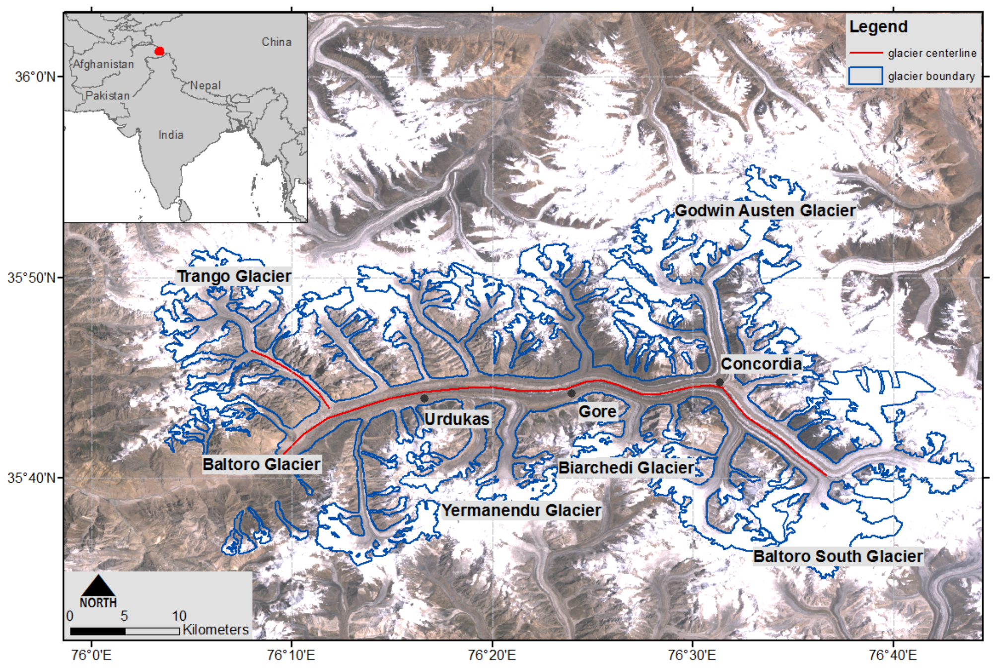
Baltoro Glacier is located in the Karakoram Range in Northern Pakistan, close to the border to China. Together with its tributaries it covers an area of approximately 660 km² (Figure 1) [7]. Above Concordia (4600 m a.s.l.), Baltoro South Glacier and Godwin Austen Glacier converge to the main Baltoro Glacier, which flows in the east-west-direction to its terminus at 3410 m a.s.l. In total, the glacier has a length of about 63 km. Surface velocities range between 120–240 m a⁻¹ at Concordia (33 km distance from terminus) and 10–40 m a⁻¹ within a 3 km distance from the terminus. Approximately 38% of Baltoro Glacier is debris covered with a thin layer of 5–15 cm at Concordia, a layer of 30–40 cm at Urdukas, and and an approximately 1 m thick layer of debris [7,9]. Debris-covered glaciers are often characterized by the existence of supraglacial lakes and ice cliffs, which at Baltoro Glacier frequently occur on the lower tongue [7,14,15,16,17]. Additionally, there exists ice sails over a large part of the ablation area. Ice sails are defined as isolated clean ice melt features with clearly defined ridges and broadly flat faces, which protrude from the debris-covered glacier for several years [7,16]. Baltoro Glacier is a dendritic glacier and is nourished from short high-elevation basins above 5400 m and avalanches from steep valley slopes [7,18].

The Karakoram is characterized by a mid-latitude high-mountain climate with cold winters and mild summers and is mainly dominated by three different climate systems: (1) the westerlies with dominant snowfall during winter and spring, contributing two-thirds of the yearly snowfall in high altitudes, (2) the Indian summer monsoon with increasing precipitation, decreasing temperatures, and increasing cloud coverage during the summer monsoon season (June to September), contributing to snow accumulation in the higher reaches of the glacier, and (3) the usually rather stable Tibetan Anticyclone [1]. In case of an irregular weakening of this system, incursions of the Indian summer monsoon with large amounts of precipitation in the central Karakoram are possible [1,5]. The mean annual precipitation is about 1600 mm a⁻¹ at 5300 m a.s.l. in the Godwin Austen region and at 5500 m a.s.l. in the Baltoro South region. As the mean daytime temperature during summer is close to the freezing point at 5400 m a.s.l., most of the precipitation deposits as snow above this elevation [7].

3. Data

For the calculation of surface velocities we used sequences of SAR images in single look complex (SLC) format, acquired by ERS-1/2, ENVISAT ASAR, ALOS PALSAR-1, TerraSAR-X, TanDEM-X, and Sentinel-1 (

Table 1. Overview of the SAR sensor characteristics and the parameters used for the velocity tracking. The pass directions are abbreviated as A for Ascending and D for Descending. Pixel spacings in range (r) and azimuth (az) refer to the raw data and are approximate values. The tracking patch and step size are given in number of pixels (p).

	ERS-1/2	ENVISAT ASAR	ALOS PALSAR-1	TerraSAR-X/TanDEM-X	Sentinel-1
Mode	Image Mode	Image Mode	Fine Mode	StripMap	Interferometric
	(IMS)	(IMS)	(FBS and FBD)	(SM)	Wide Swath (IW)
Pixel Spacing (r × az)	20 × 4 m	20 × 4 m	7 × 3 m	<2 × 2 m	>2 × 14 m
Acquisition Period	1992–1999	2003–2010	2007–2011	2009–2016	2014–2017
Number of Acquisitions	7	35	15	62	41
Min. Temporal Baseline (d)	35	35	46	11	24/12
Orbit	377	377	526	75/98/151	27/34
Pass Direction	D	D	A	D/A/D	A/D
Tracking patch size (p × p)	64 × 320	64 × 320	64 × 192	256 x 256	320 x 64
Tracking step size (p × p)	5 × 25	5 × 25	10 × 30	25 × 25	25 × 5

). For the Karakoram, the first SAR acquisitions were available from ERS-1/2 in winter 1992, winter 1993, and summer 1999. The ENVISAT mission provides a continuous time series of image pairs between 2003 and 2010 that has been filled by data of ALOS PALSAR-1, acquired during 2006–2011. Since 2012, TerraSAR-X and TanDEM-X have provided repeat pass imagery at temporal baselines of up to 11 days, and Sentinel-1 has regularly mapped the region every 24 (2014–2017) and 12 days (since 2017), which enables detailed observations of short-term surface velocity changes. A summary of the specifications of the SAR sensors is given in Table 1. The 90 m C-band digital elevation model (USGS release 2.0) acquired during the Shuttle Radar Topography Mission (SRTM) in February 2000 served as a topographic reference for geocoding and ortho-rectification of the surface velocity maps.

Supraglacial lakes were mapped from multi-spectral Landsat-5 Thematic Mapper (TM), Landsat-7 Thematic Mapper Plus (ETM+), and Landsat-8 Operational Land Imager (OLI) Level-2 data (path 148, row 35) with a spatial resolution of 30 m, and ASTER (Advanced Spaceborne Thermal Emission and Reflection Radiometer) Level-1 Precision Terrain Corrected Registered At-Sensor Radiance (AST_L1T) imagery with a spatial resolution of 15 m. Hence, both data sets are atmospherically corrected. Furthermore, only data without cloud coverage over Baltoro Glacier are used. Between 1991 and 2017, 23 scenes acquired in the summer season (June to September) are available. The time series is not continuous and for some years data gaps exist. However for 2000, 2002, 2004, and 2011 two, and for 2016 even three, acquisitions are available.

In order to analyze the connection between surface velocities and meteorological conditions, monthly accumulated precipitation data of the Tropical Rainfall Measurement Mission (TRMM_3B43, Version 7) and re-analysis temperature data of ERA-Interim were used [12,13]. Both data span the period from 1998 to 2017 and are available in a 0.25${}^{\circ }$× 0.25${}^{\circ }$ grid (WGS84).

4. Methodology

4.1. Surface Velocities

Surface velocities were calculated by applying an intensity offset tracking algorithm to consecutive pairs of co-registered SAR intensity images [19]. Here, the horizontal ice displacement was derived by determining the intensity cross correlation peaks between patches of an image pair using a moving window approach. In contrast to interferometry, intensity offset tracking does not require phase coherence, but relies on the presence of nearly identical features in two subsequent SAR intensity images (feature tracking). This makes the technique also applicable in cases of longer temporal baselines between both acquisitions (e.g., >100 days). However, if phase coherence is maintained over shorter temporal baselines, the speckle pattern of the images is correlated and intensity offset tracking is performed at higher accuracy (speckle tracking). Depending on the temporal baseline, the sensor specifications, and the expected displacement, data-specific tracking patch sizes and step sizes have to be defined (Table 1). Velocity estimates of low confidence were discarded during the tracking procedure using a cross-correlation coefficient threshold of 0.1. The resulting velocity fields were smoothed by applying a 7 × 7 median filter [20,21]. Profiles of surface velocities were obtained by extracting the values along the glacier’s centerline (Figure 1, red line). The methodology of deriving surface velocity from multi-mission SAR data is explained in more detail in Rankl et al. [10] and Friedl et al. [22].

4.2. Accuracy Assessment of Surface Velocities

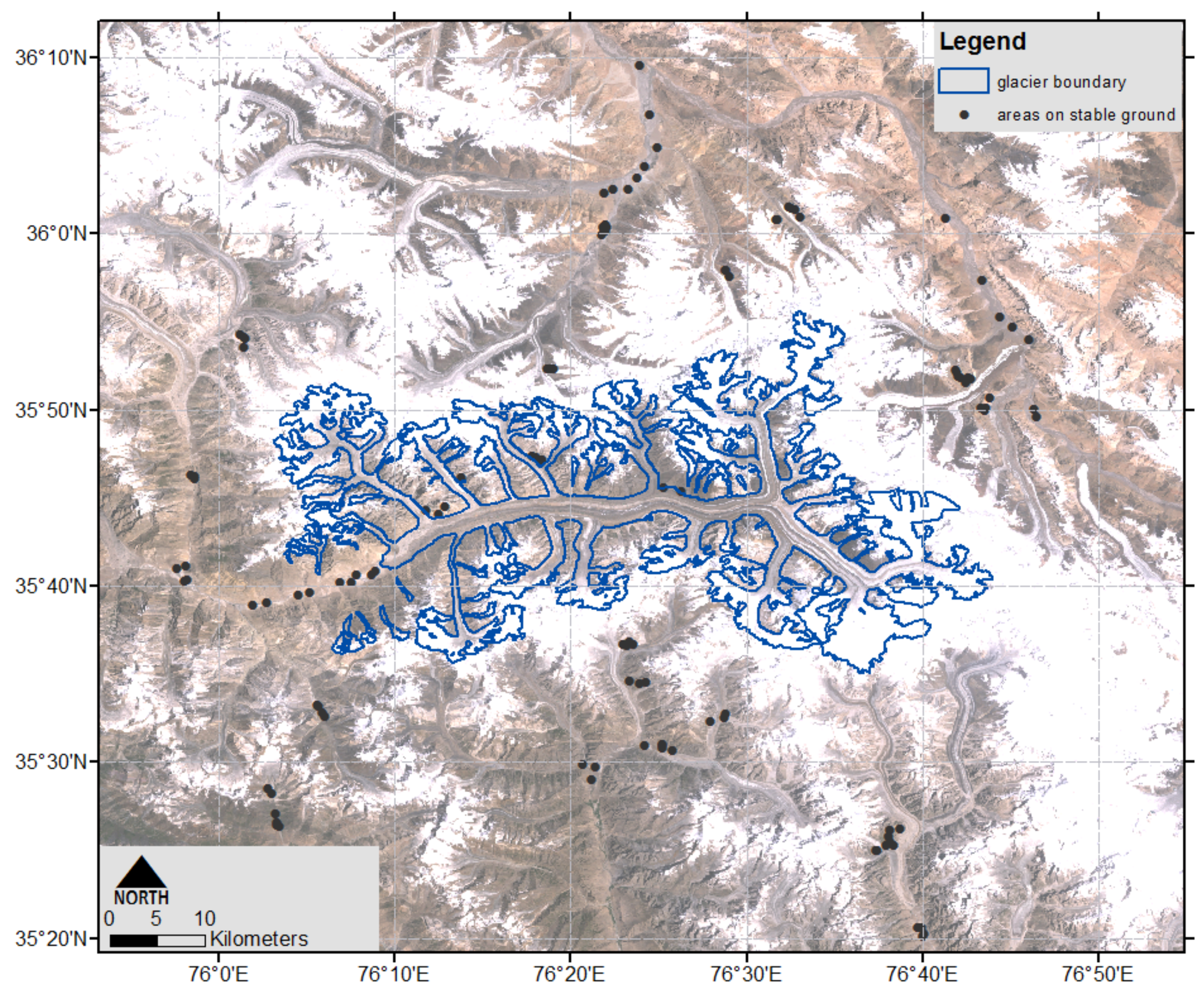
The accuracy of the calculated surface velocities mainly depends on the characteristics of the glacier, the intensity offset tracking algorithm, and the SAR data. The first includes glacier topography, roughness, and feature stability, the second includes tracking patch size, step size, search radius, temporal baseline, and co-registration accuracy and the latter acquisition includes geometry, orbit, pass direction, spatial resolution, and wavelength. Similar to Rankl et al. [10], the accuracy of surface velocities was estimated by extracting displacement values at 121 well distributed stable (non-moving) points over non-glaciated ground (Figure A1). The number of control points varied between 10 for TerraSAR-X and 72 for Sentinel-1 due to different spatial coverages of the data. For each displacement field, the mean accuracy and the corresponding standard deviation (±1$\sigma$) were calculated (

Table A1. Accuracy assessment (m a⁻¹) and the standard deviation (sd) ±1$\sigma$ of the processed surface velocities with $\Delta$t in days as the time interval in days between repeat SAR acquisitions. As TerraSAR-X and TanDEM-X data are identical in construction, both data sets are categorized as TerraSAR-X. The table is continued on the following pages.

Date	Sensor	Orbit	$\mathbf{\Delta }$ t (d)	Accuracy (m a−1)	sd (±1$\mathit{\sigma }$)
19.11.1992–24.12.1992	ERS-1/2	377	35	26.61	21.40
24.12.1992–28.01.1993	ERS-1/2	377	35	27.93	18.58
28.01.1993–04.03.1993	ERS-1/2	377	35	15.06	16.62
04.03.1993–08.04.1993	ERS-1/2	377	35	32.36	15.15
16.05.1999–20.06.1999	ERS-1/2	377	35	20.43	12.79
31.10.2004–05.12.2004	Envisat ASAR	377	35	12.37	12.28
09.01.2005–13.02.2005	Envisat ASAR	377	35	24.43	28.64
13.02.2005–20.03.2005	Envisat ASAR	377	35	22.73	30.20
24.04.2005–29.05.2005	Envisat ASAR	377	35	42.68	27.99
29.05.2005–03.07.2005	Envisat ASAR	377	35	44.97	27.19
03.07.2005–11.09.2005	Envisat ASAR	377	70	15.94	13.61
11.09.2005–16.10.2005	Envisat ASAR	377	35	17.69	17.81
16.10.2005–20.11.2005	Envisat ASAR	377	35	12.22	15.67
20.11.2005–25.12.2005	Envisat ASAR	377	35	11.48	19.91
29.01.2006–05.03.2006	Envisat ASAR	377	35	45.04	32.91
05.03.2006–14.05.2006	Envisat ASAR	377	70	11.01	13.63
14.05.2006–18.06.2006	Envisat ASAR	377	35	10.00	10.54
18.06.2006–23.07.2006	Envisat ASAR	377	35	28.85	26.13
23.07.2006–27.08.2006	Envisat ASAR	377	35	23.3	14.55
27.08.2006–10.12.2006	Envisat ASAR	377	105	10.29	9.50
10.12.2006–18.02.2007	Envisat ASAR	377	70	10.62	22.11
23.12.2006–07.02.2007	ALOS PALSAR-1	526	46	28.25	15.07
07.02.2007–10.08.2007	ALOS PALSAR-1	526	184	20.44	13.45
18.02.2007–25.03.2007	Envisat ASAR	377	35	32.14	26.03
25.03.2007–29.04.2007	Envisat ASAR	377	35	37.71	24.54
10.08.2007–25.09.2007	ALOS PALSAR-1	526	46	4.47	7.38
16.09.2007–25.11.2007	Envisat ASAR	377	70	8.11	4.62
25.09.2007–26.12.2007	ALOS PALSAR-1	526	92	5.76	6.18
26.12.2007–10.02.2008	ALOS PALSAR-1	526	46	51.07	23.99
10.02.2008–27.03.2008	ALOS PALSAR-1	526	46	9.96	9.04
27.03.2008–27.06.2008	ALOS PALSAR-1	526	92	35.33	19.08
12.05.2008–27.06.2008	ALOS PALSAR-1	526	46	86.83	46.88
27.06.2008–28.12.2008	ALOS PALSAR-1	526	184	23.77	14.81
28.12.2008–12.02.2009	ALOS PALSAR-1	526	46	22.85	11.13
18.01.2009–22.02.2009	Envisat ASAR	377	35	16.92	18.59
12.02.2009–30.06.2009	ALOS PALSAR-1	526	138	6.95	4.39
22.02.2009–29.03.2009	Envisat ASAR	377	35	31.99	26.32
07.06.2009–20.09.2009	Envisat ASAR	377	105	4.75	3.27
30.06.2009–15.08.2009	ALOS PALSAR-1	526	46	95.45	55.51
15.08.2009–31.12.2009	ALOS PALSAR-1	526	138	15.41	8.90
20.09.2009–25.10.2009	Envisat ASAR	377	35	33.75	21.58
25.10.2009–29.11.2009	Envisat ASAR	377	35	12.59	15.97
29.11.2009–14.03.2010	Envisat ASAR	377	105	6.27	5.73
31.12.2009–15.02.2010	ALOS PALSAR-1	526	46	18.49	8.74
14.03.2010–23.05.2010	Envisat ASAR	377	70	9.50	13.68
03.07.2010–18.08.2010	ALOS PALSAR-1	526	46	16.46	16.46
18.08.2010–03.01.2011	ALOS PALSAR-1	526	138	18.40	11.24
03.01.2011–18.02.2011	ALOS PALSAR-1	526	46	40.38	21.37
12.11.2011–04.12.2011	TerraSAR-X	75	22	0.75	0.60
04.12.2011–06.01.2012	TerraSAR-X	75	33	0.42	0.16
06.01.2012–06.05.2012	TerraSAR-X	75	121	0.63	0.29
20.02.2012–26.04.2012	TerraSAR-X	98	66	6.45	2.57
06.05.2012–07.10.2012	TerraSAR-X	75	154	1.08	0.44
07.10.2012–27.02.2013	TerraSAR-X	75	143	0.45	0.24
08.10.2012–27.05.2013	TerraSAR-X	98	231	2.54	0.73
09.01.2013–07.04.2013	TerraSAR-X	75	88	0.54	1.76
27.02.2013–10.03.2013	TerraSAR-X	75	11	1.24	5.01
27.02.2013–12.04.2013	TerraSAR-X	75	44	1.96	0.59
10.03.2013–12.04.2013	TerraSAR-X	75	33	2.68	0.92
22.03.2013–21.07.2013	TerraSAR-X	98	121	2.51	1.91
12.04.2013–26.05.2013	TerraSAR-X	75	44	0.81	1.52
27.08.2013–07.09.2013	TerraSAR-X	151	11	26.63	14.43
19.03.2014–10.04.2014	TerraSAR-X	75	22	6.78	3.79
19.03.2014–24.05.2014	TerraSAR-X	75	66	0.61	1.39
30.03.2014–24.05.2014	TerraSAR-X	75	55	5.45	2.04
10.04.2014–24.05.2014	TerraSAR-X	75	44	3.14	1.32
11.04.2014–05.06.2014	TerraSAR-X	98	55	8.06	2.25
11.04.2014–23.09.2014	TerraSAR-X	98	165	1.17	1.75
22.04.2014–16.06.2014	TerraSAR-X	98	55	17.38	9.52
03.05.2014–27.06.2014	TerraSAR-X	98	55	11.24	6.37
05.06.2014–23.09.2014	TerraSAR-X	98	110	1.59	1.85
18.12.2014–11.01.2015	Sentinel-1	27	24	3.86	8.52
11.01.2015–04.02.2015	Sentinel-1	27	24	5.56	16.07
29.04.2015–23.05.2015	Sentinel-1	27	24	5.31	7.22
23.05.2015–16.06.2015	Sentinel-1	27	24	5.68	6.29
16.06.2015–10.07.2015	Sentinel-1	27	24	4.51	8.21
12.08.2015–23.08.2015	TerraSAR-X	151	11	13.30	7.95
02.10.2015–26.10.2015	Sentinel-1	27	24	8.44	10.26
19.11.2015–13.12.2015	Sentinel-1	27	24	9.76	7.71
13.12.2015–06.01.2016	Sentinel-1	27	24	8.38	10.24
06.01.2016–30.01.2016	Sentinel-1	27	24	13.46	13.68
30.01.2016–23.02.2016	Sentinel-1	27	24	10.6	14.08
23.02.2016–18.03.2016	Sentinel-1	27	24	10.00	15.03
18.03.2016–11.04.2016	Sentinel-1	27	24	10.17	14.62
19.03.2016–30.03.2016	TerraSAR-X	151	11	14.83	10.89
30.03.2016–13.05.2016	TerraSAR-X	151	44	4.34	1.43
10.04.2016–24.05.2016	TerraSAR-X	151	44	6.60	14.68
11.04.2016–05.05.2016	Sentinel-1	27	24	9.85	12.83
21.04.2016–18.07.2016	TerraSAR-X	151	88	2.03	2.69
05.05.2016–29.05.2016	Sentinel-1	27	24	10.47	5.96
13.05.2016–26.06.2016	TerraSAR-X	151	44	1.67	1.59
18.05.2016–11.06.2016	Sentinel-1	34	24	3.75	2.60
24.05.2016–07.07.2016	TerraSAR-X	151	44	1.71	1.42
11.06.2016–29.07.2016	Sentinel-1	34	48	3.19	1.70
26.06.2016–09.08.2016	TerraSAR-X	151	44	2.32	1.58
07.07.2016–20.08.2016	TerraSAR-X	151	44	1.36	0.54
16.07.2016–09.08.2016	Sentinel-1	27	24	3.51	6.05
18.07.2016–31.08.2016	TerraSAR-X	151	44	1.85	0.81
09.08.2016–02.09.2016	Sentinel-1	27	24	6.59	5.17
09.08.2016–11.09.2016	TerraSAR-X	151	33	0.97	0.52
20.08.2016–22.09.2016	TerraSAR-X	151	33	3.20	3.63
31.08.2016–03.10.2016	TerraSAR-X	151	33	6.85	2.11
02.09.2016–26.09.2016	Sentinel-1	27	24	9.24	7.63
11.09.2016–14.10.2016	TerraSAR-X	151	33	6.68	6.85
22.09.2016–25.10.2016	TerraSAR-X	151	33	1.15	0.97
26.09.2016–20.10.2016	Sentinel-1	27	24	3.61	6.89
03.10.2016–05.11.2016	TerraSAR-X	151	33	1.93	1.01
14.10.2016–16.11.2016	TerraSAR-X	151	33	2.98	2.10
20.10.2016–13.11.2016	Sentinel-1	27	24	2.84	2.46
25.10.2016–27.11.2016	TerraSAR-X	151	33	3.16	3.66
05.11.2016–08.12.2016	TerraSAR-X	151	33	3.65	2.37
13.11.2016–07.12.2016	Sentinel-1	27	24	5.42	12.76
07.12.2016–31.12.2016	Sentinel-1	27	24	3.38	6.92
31.12.2016–24.01.2017	Sentinel-1	27	24	4.53	10.48
24.01.2017–05.02.2017	Sentinel-1	27	12	15.76	26.81
05.02.2017–17.02.2017	Sentinel-1	27	12	10.85	17.88
17.02.2017–01.03.2017	Sentinel-1	27	12	14.72	19.18
01.03.2017–13.03.2017	Sentinel-1	27	12	9.44	15.43
13.03.2017–06.04.2017	Sentinel-1	27	24	17.25	13.09
06.04.2017–18.04.2017	Sentinel-1	27	12	32.28	50.22
18.04.2017–30.04.2017	Sentinel-1	27	12	11.21	22.68
30.04.2017–12.05.2017	Sentinel-1	27	12	8.71	18.70
12.05.2017–24.05.2017	Sentinel-1	27	12	11.57	13.14
24.05.2017–05.06.2017	Sentinel-1	27	12	9.67	5.94
29.06.2017–11.07.2017	Sentinel-1	27	12	8.80	8.04
11.07.2017–23.07.2017	Sentinel-1	27	12	7.71	4.65
23.07.2017–04.08.2017	Sentinel-1	27	12	8.22	8.58
04.08.2017–16.08.2017	Sentinel-1	27	12	11.92	6.40
16.08.2017–28.08.2017	Sentinel-1	27	12	6.71	4.51
28.08.2017–09.09.2017	Sentinel-1	27	12	9.71	8.87
09.09.2017–21.09.2017	Sentinel-1	27	12	4.53	5.62
21.09.2017–03.10.2017	Sentinel-1	27	12	4.86	2.91
03.10.2017–15.10.2017	Sentinel-1	27	12	7.91	7.63
15.10.2017–27.10.2017	Sentinel-1	27	12	6.78	4.61
27.10.2017–08.11.2017	Sentinel-1	27	12	6.56	4.87
08.11.2017–20.11.2017	Sentinel-1	27	12	5.86	3.27
20.11.2017–02.12.2017	Sentinel-1	27	12	7.02	8.06
02.12.2017–14.12.2017	Sentinel-1	27	12	9.42	9.49
14.12.2017–26.12.2017	Sentinel-1	27	12	8.36	7.06
26.12.2017–07.01.2018	Sentinel-1	27	12	9.82	7.49

). Based on these values, total mean accuracies for each sensor and orbit are provided in

Table 2. Accuracy of surface velocities (m a⁻¹) and standard deviation (sd) ±1$\sigma$, averaged for each sensor and orbit.

	ERS-1/2	ENVISAT ASAR	ALOS PALSAR-1	TerraSAR-X/TanDEM-X	Sentinel-1
Orbit	377	377	526	75/98/151	27/34
Accuracy (m a−1± 1$\sigma$)	26.6 ± 6.7 m a−1	16.4 ± 12.6 m a−1	20.4 ± 26.3 m a−1	1.1 ± 2.0 m a−1/4.5 ± 5.7 m a−1/3.0 ± 4.7 m a−1	8.4 ± 4.8 m a−1/3.5 ± 0.4 m a−1

.

4.3. Supraglacial Lakes Detection

Supraglacial lakes were classified by applying a threshold on the the Normalized Difference Water Index (NDWI) calculated for Landsat and ASTER imagery, acquired in 1991–2017:

$$\begin{array}{c}\hfill NDWI=\left(\frac{GREEN-NIR}{GREEN+NIR}\right)\end{array}$$

(1)

For the Landsat acquisitions, the NDWI is based on the ratio between the reflectance of the green (Band 2 with 0.52 $\mathsf{\mu }$m–0.60 $\mathsf{\mu }$m for Landsat-5 and 7, Band 3 with 0.533 $\mathsf{\mu }$m–0.673 $\mathsf{\mu }$m for Landsat-8, respectively) and the near-infrared band (Band 4 with 0.77 $\mathsf{\mu }$m–0.90 $\mathsf{\mu }$m for Landsat-5 and 7, Band 5 with 0.851 $\mathsf{\mu }$m–0.879 $\mathsf{\mu }$m for Landsat-8, respectively) [23]. For the ASTER imagery, Band 1 (0.52 $\mathsf{\mu }$m–0.60 $\mathsf{\mu }$m) is the green band and Band 3 (0.76 $\mathsf{\mu }$m–0.86 $\mathsf{\mu }$m) is the near-infrared band [24,25].

Applying the band combinations SWIR and NIR [26], SWIR and Green [27], and green and SWIR [28] led to similar results. In addition, ASTER lacks the blue band and the ASTER data of 30 May 2011 and 20 August 2012 lacks the SWIR band. Since we aimed at a consistent comparison of lakes derived from Landsat and ASTER data, we finally chose the combination of green and NIR, which is the most common used band combination [24,25]. According to McFeeters et al. [23], all pixels with an NDWI >0 can be assigned to the land cover type “water.” Empirical analysis in our region of interest showed that, for Landsat imagery, an NDWI threshold of 0.1 is well suited for water detection, as it reduces the misclassification of snow. Since all Landsat scenes were acquired in the same orbit geometry, a uniform threshold was used for all Landsat scenes. The data gap since 2003 due to the failure of the Scan Line Corrector of Landsat-7 ETM+ was filled with available ASTER data. Compared to the 30 m spatial resolution of Landsat data, ASTER has a higher spatial resolution (15 m), which allows for a better detection of small ponds. As ASTER scenes were acquired at different orbit geometries and varying acquisition times, an individual threshold between 0.03 and 0.18 was applied to every scene. Misclassified snow cover on the tributaries Yermanendu Glacier and Biarchedi Glacier, as well as ice sails [16] were manually removed. For each resulting lake-mask, the total number of supraglacial lakes and their overall total area were determined. Potential lakes smaller than 1800 m${}^2$ (2 pixels in area for Landsat and 8 pixels in area for ASTER) were omitted in order to minimize the possibility of false positives. The classification results were visually compared with the corresponding optical data of Landsat, ASTER, and the calculated NDWI, respectively. Due to the sparse stock of optical data, a meaningful accuracy assessment was not possible. Though Bolch et al. compared NDWI-derived supraglacial lakes from IKONOS and ASTER imagery and determined a deviation of less than 10% for the lake area due to small ponds, which were not detectable in acquisitions of coarser resolutions [25].

4.4. Precipitation and Temperature

One of the most common measures of precipitation surpluses and deficits (droughts) is the Standardized Precipitation Index (SPI) [29]. The calculation of the SPI for a certain location is based on a long-term precipitation record that is fitted to a probability distribution and subsequently transformed into a normal distribution. Hence, the mean SPI for a specific location and desired period is zero. SPI values from −0.99 to +0.99 indicate near normal precipitation. Surpluses are expressed by positive SPI values, whereas SPI values from +1.0 to +1.49 denote moderately wet, SPI values from +1.5 to +1.99 very wet, and SPI values >+2.0 extremely wet periods. Droughts are indicated by a negative SPI. Values between −1.0 and −1.49 indicate moderately dry phases, whereas SPI values from −1.5 to −1.99 and <−2.0 denote severely and extremely dry periods, respectively [29,30,31,32]. The reliability of the TRMM data for the Karakoram had been previously confirmed by Quincey et al. [9]. The temperature anomaly can be described with the Standardized Temperature Index (STI). The STI bases on the same principle as SPI. STI values from −0.99 to +0.99 indicate near normal temperatures. Warm periods are represented by positive STI values, whereas STI values from +1.0 to +1.49 mean moderately hot, STI values from +1.5 to +1.99 very hot, and STI values >+2.0 extremely hot periods. Cold periods are presented by a negative STI. Values between −1.0 and −1.49 indicate moderately cold periods, whereas STI values from −1.5 to −1.99 and <−2.0 mean very and extremely cold periods, respectively [33]. In our study, we aggregated precipitation and temperature over a period of 3 months, as this reflects short- and medium-term moisture conditions and provides a seasonal estimation of precipitation [34].

5. Results

5.1. Annual Surface Velocities

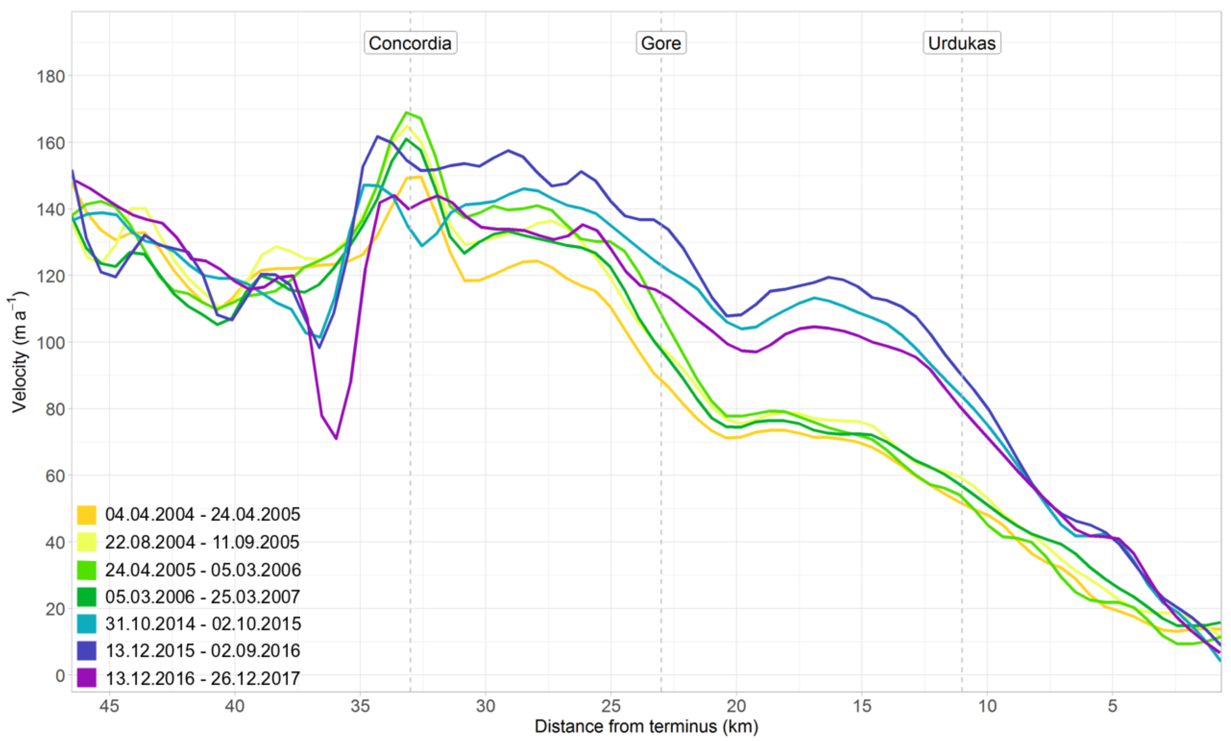
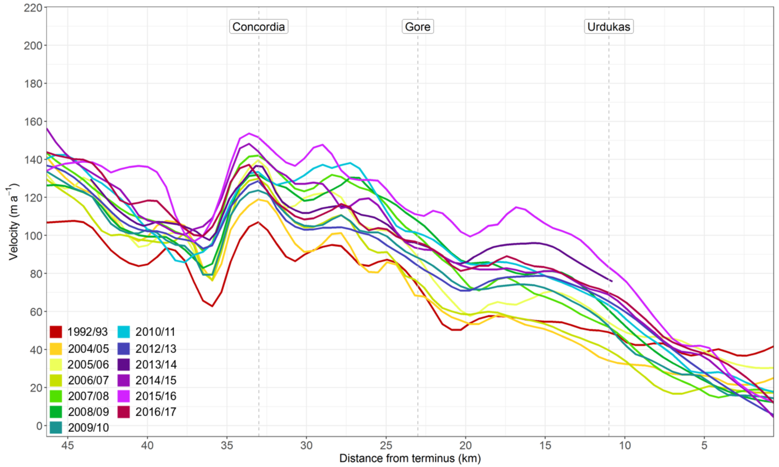
Annual centerline velocities, calculated for 2004–2017, represent recent long-term annual velocity variations of the glacier (Figure 2). To minimize seasonal effects, only data pairs acquired in the same season were used for the calculations. In order to compare our results with Quincey et al. [9], we used the same datasets for the timespan between 2004 and 2007. Unfortunately, at the time of processing, the ERS-1/2 data from 20 April 1996 and the ENVISAT ASAR data from 03 August 2003 and 13 April 2008 were not available in the ESA data archive anymore. Hence, the respective annual pairs from 8 April 1993 to 20 April 1996, from 3 August 2003 to 22 August 2004, and from 5 March 2006 to 13 April 2008 presented in Quincey et al. [9] are missing in our study. Thus, the annual displacements from 4 April 2004 to 24 April 2005, from 22 August 2004 to 11 September 2005, from 24 April 2005 to 5 March 2006, and from 5 March 2006 to 25 March 2007 were derived from ERS-1/2 scenes with an accuracy of 3.5 ± 2.7 m a⁻¹. Additionally, the annual velocities from 31 October 2014 to 2 October 2015, 13 December 2015 to 2 September 2016, as well as 31 December 2016 to 26 December 2017 were calculated from Sentinel-1 acquisitions with an accuracy of 1.1 ± 0.5 m a⁻¹.

The velocity profiles reveal a characteristic general pattern, which is similar for all investigated annual periods. Peak velocities of up to ~ 170 m a⁻¹ are found at Concordia (33 km distance from terminus), which decrease to slightly lower, but almost steady values of up to ~160 m a⁻¹ between Concordia and Gore (29–25 km). The generally higher velocities at Concordia are due to the confluence of the two glacier branches Godwin Austin from the north and Baltoro South from the south as well as the resulting higher mass flux. Between Gore and Urdukas (24–20 km), velocities decrease quite rapidly to maximum values of ~110 m a⁻¹. The lower part of the glacier (approximately the last 15 km distance to the glacier snout) is characterized by continuously decreasing velocities trending towards zero. The annual surface velocities from 2004 to 2007 were very similar to those derived by Quincey et al. [9] (maximum velocity differences of ~20 m a⁻¹), documenting the validity of our approach. However, significant differences in the velocity pattern between the periods 2004–2007 and 2014–2017 were evident: (1) at Concordia (33 km) surface velocities decreased by 20–40 m a⁻¹, (2) between Concordia and Gore (29–25 km) velocities increased by up to 30 m a⁻¹, (3) between Gore and Urdukas (23–11 km) the glacier accelerated by up to 40 m a⁻¹, and (4) at the terminus (11–0 km) an increase by 10–20 m a⁻¹ as well as a steeper gradient were detected.

5.2. Summer and Winter Surface Velocities

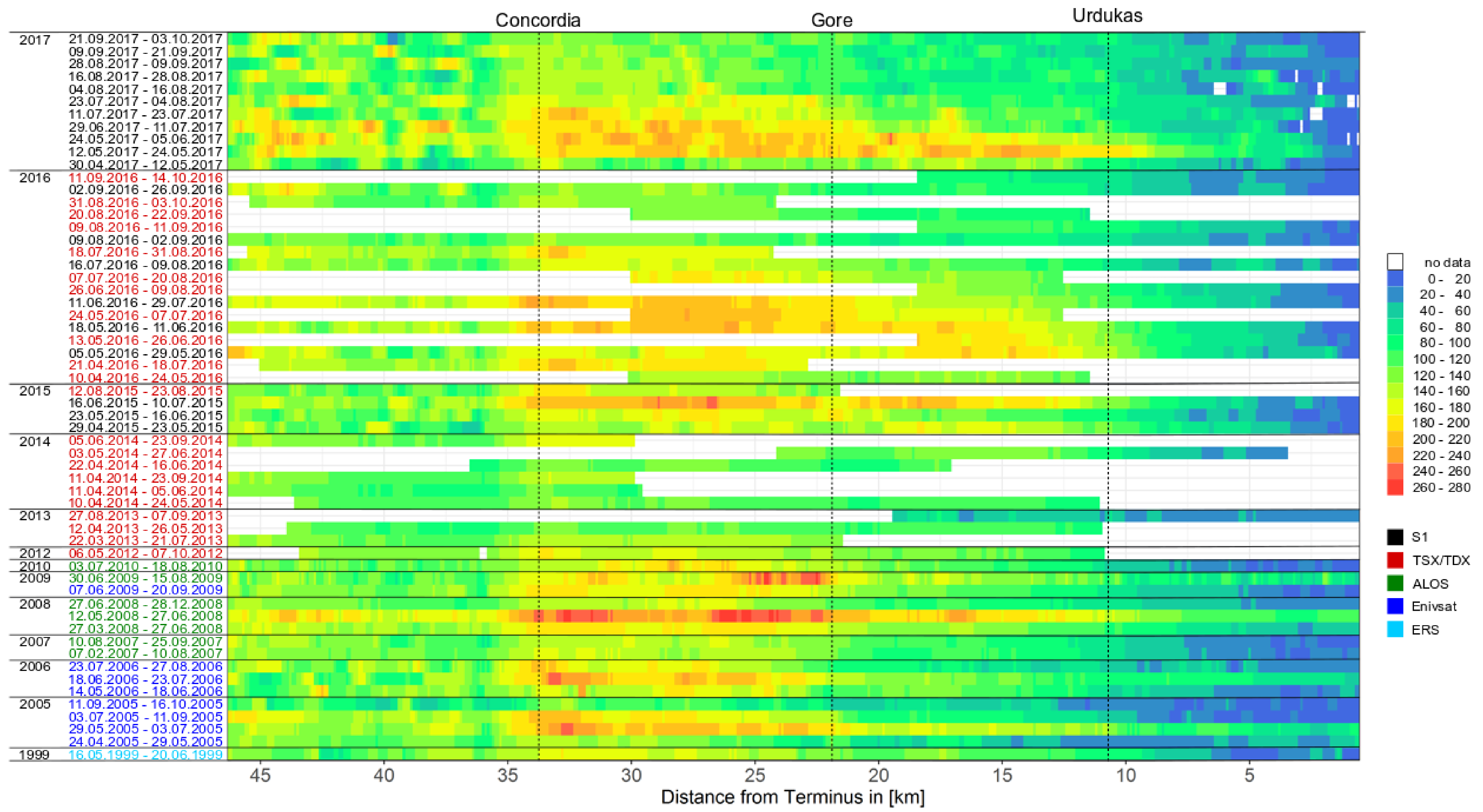
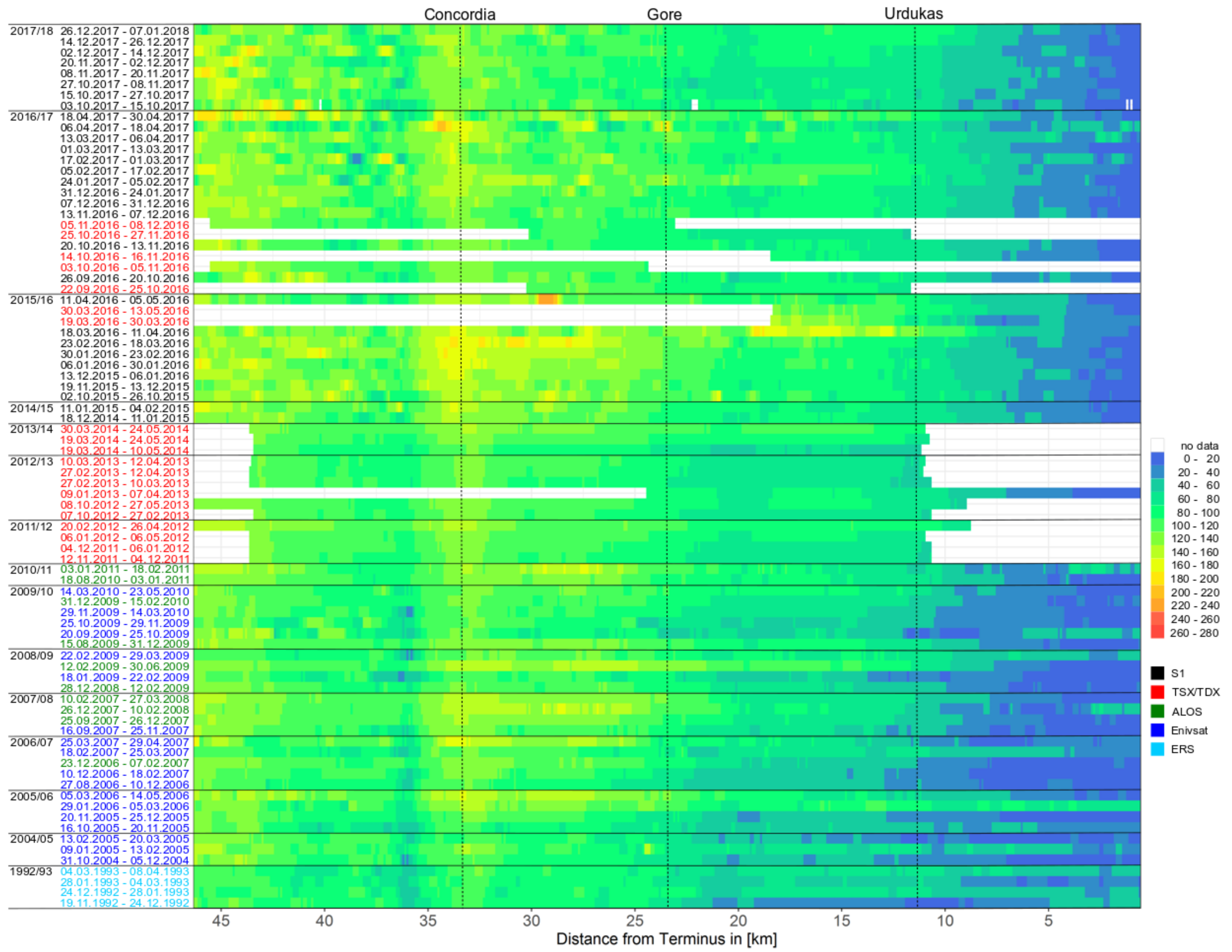
In order to investigate seasonal differences between 1992 and 2017, we calculated mean summer (Figure 3) and winter surface velocities (Figure 4). Therefore, all available velocities were averaged to profiles of mean summer (Figure 3) and winter velocities (Figure 4) in dependence of the acquisition date. Velocity fields were assigned to a season according to the center date of the corresponding image pair. Based on the general occurrence and absence of melt conditions, the summer season was defined to range from May to September and the winter season from October to April, respectively. Averaging a stack of multiple velocity fields to a single velocity field utilizes the redundancy of information, bridges data gaps, minimizes outliers, and delivers a more robust result [20]. However, it must be noted that number and dates of acquisitions may influence the result. For example, summer velocities in 2007 are based on just one velocity field (10 August to 25 September 2007). Since this late summer period is usually characterized by lower velocities, the mean summer velocities of 2007 may be underestimated. In contrast, mean summer velocities for the year 2017 were based on a continuous time series of eleven surface velocity fields, covering the entire summer season from May to September. Figure 5 and Figure 6 show the number and dates of acquisitions used to calculate the mean summer and winter velocities for each year, as well as the corresponding sensors.

In general, the seasonal velocities show a higher variability in summer (Figure 3) than in winter (Figure 4). Along Baltoro South Glacier (47–35 km distance from terminus), summer velocities range between 100 and 160 m a⁻¹, with a local minimum of 87 m a⁻¹ at 42 km in 1999. At Concordia (33 km), summer velocities increased to up to 140–200 m a⁻¹ with the highest values found in 2005, 2006, 2008, 2009, and 2016 and the lowest values in 2010, 2013, and 2014. Downstream of Concordia, the velocity decreased towards the terminus to values of 110–205 m a⁻¹ between Concordia and Gore (27–23 km), and 60–160 m a⁻¹ between Gore and Urdukas (17–13 km). Maximum summer velocities were up to 205 m a⁻¹ between Concordia and Gore in 2006, 2008, 2009, and 2010, and 120–160 m a⁻¹ between Gore and Urdukas in 2015.

No clear overall trend was recognizable for the averaged summer velocities over the last twenty years. In contrast, year to year variations with considerable ranges seem to dominate (Figure 3). At Concordia, the lowest summer mean velocities were observed in 2013 and 2014 and the highest velocities were measured in 2005, 2006, 2008, 2009, and 2016. Between Concordia and Gore, higher velocities were observed in 2006, 2008, 2009, and 2010, with exceptional high values of >200 m a⁻¹ at Gore in 2010. In 2015, the summer velocities between Concordia and Urdukas were almost constant above 160 m a⁻¹, with a strong decrease downstream of Urdukas was found. Higher summer velocities between Concordia and Urdukas were also observed in 2016 and 2017. However, due to the higher temporal resolution of the Sentinel-1 data, the averaged summer velocity of both years was attenuated. For 2015–2017, a steeper gradient of the surface velocity at the terminus (7–0 km) was recognizable, which can be also seen in Figure 2.

The winter velocities (Figure 4) are generally lower (<160 m a⁻¹) and show a more homogeneous and smooth shape. Along Baltoro South Glacier (47–35 km), the velocities ranged between 60 and 155 m a⁻¹ with a local minimum of 60–110 m a⁻¹ just upstream of Concordia (35 km). At Concordia, the velocities increased to 113–155 m a⁻¹ with minimum values in 1992/1993 and 2013/14 and peak values in 2014/2015 and 2015/2016. At Gore (23 km), the displacement rate decreased to 80–130 m a⁻¹ and at Urdukas to 40–85 m a⁻¹. In winter 2015/2016, the peak between Gore and Urdukas with values of 117 m a⁻¹ was much higher than the average. Since 2012, a trend towards higher velocities between Gore and the terminus as well as a steeper gradient of the deceleration at the terminus (7–0 km) was recognizable.

The averaged summer and winter velocities indicate how seasonal velocities varied since 1992. However, information on intra-seasonal velocity variations is blurred by the averaging method. Therefore, we present seasonal heat maps containing all single summer and winter velocities (Figure 5 and Figure 6). Here, the characteristic pattern of lower velocities just upstream of Concordia (35 km), maximum velocities at Concordia, and decreasing velocities towards the terminus are well recognizable. Figure 5 shows that increased velocities were typically observed between May and July, with highest values in 2005 (180–255 m a⁻¹), 2006 (180–255 m a⁻¹), 2008 (200–280 m a⁻¹), 2009 (180–280 m a⁻¹), 2015 (220–250 m a⁻¹), 2016 (180–240 m a⁻¹), and 2017 (200–240 m a⁻¹). Figure 5 illustrates that in 2008, 2009, 2015, 2016, and 2017 higher velocities ranged from Concordia to Urdukas, whereas in 2005 and 2006 acceleration was only found between Concordia and Gore. Due to the high temporal resolution of the Sentinel-1 data, surface velocities in 2017 can be analyzed in detail: from 12 May to 24 May the velocity increased from 110–146 to 180–220 m a⁻¹ between Concordia and Urdukas, from 24 May to 11 July the velocities remained stable in a range of 145–220 m a⁻¹, whereas the extent of high velocities decreased and was restricted to Concordia and Gore. From 11 July to 4 August the velocities slowed down to 90–145 m a⁻¹ and after 4 August the glacier returned to its average velocity of 70–110 m a⁻¹. In addition, since 2010, an increase of the velocities from 0–20 to 20–40 m a⁻¹ on the lower glacier tongue (10–5 km) is recognizable.

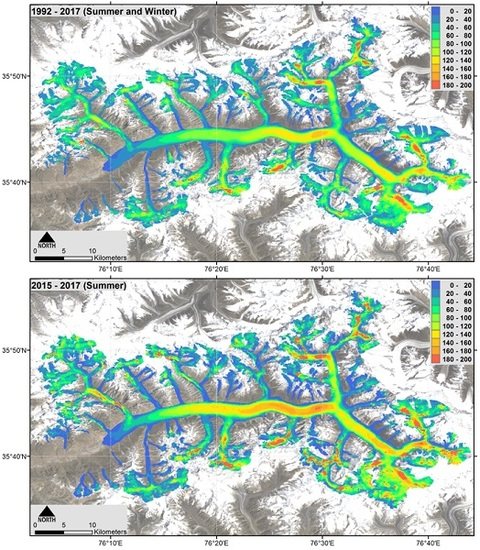
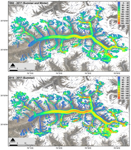
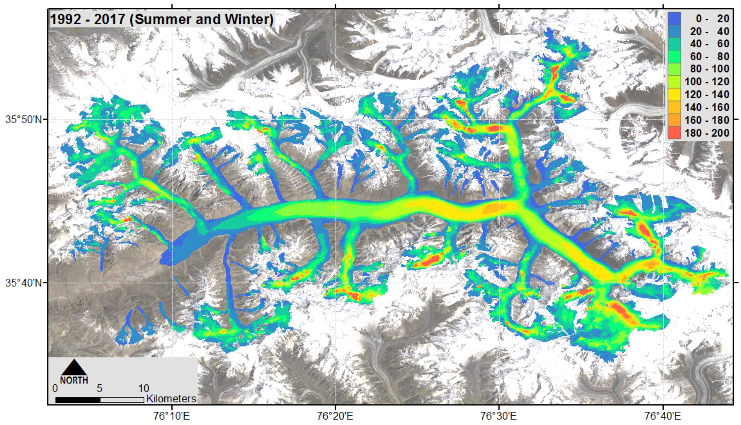
Additionally, the averaged velocity fields for both periods 1992–2017 (summer and winter) and 2015–2017 (summer) are displayed in Figure A2 and Figure A3 in the supplementary material. Both figures show the impressive increase in the surface velocity from 80–150 m a⁻¹ to 120–190 m a⁻¹ between Urdukas and Concordia in the years 2015 to 2017.

The high resolution time series of summer and winter velocities additionally indicated accelerations of the Trango Glacier (

Table 3. Time period and the mean value of the accelerations (m a⁻¹) of Trango Glacier as extracted along the profile shown in Figure 1. Note that the date refers to the acquisition date of the SAR pair used for the calculation of the displacement field.

Time Period	Surface Velocity (m a−1)
12.10.2003–16.11.2003	165–255
10.08.2007–25.09.2007	140–220
26.12.2007–27.03.2008	110–170
03.01.2011–18.02.2001	180–255
09.09.2012–25.11.2012	220–255
09.01.2013–07.04.2013	200–255
27.08.2013–07.09.2013	200–255
16.06.2015–10.07.2015	200–255
19.03.2016–14.10.2016	165–255
12.05.2017–24.05.2017	146–220

). As these accelerations affect the surface velocity of Baltoro Glacier, they appear in Figure 2, Figure 3 and Figure 4 as small velocity peaks near the terminus of Baltoro Glacier (5 km).

5.3. Supraglacial Lakes

Table 4. Total number and lake area (km${}^2$) of the supraglacial lakes for the years 1991–2017.

Date	Sensor	Total Number	Lake Area (km${}^2$)
02.07.1991	TM	216	1.62
07.07.1993	TM	202	1.40
26.07.1994	TM	153	0.99
01.09.1996	TM	74	0.51
18.07.1997	TM	178	1.38
07.09.1998	TM	168	1.07
16.06.2000	ETM+	170	1.27
27.08.2000	TM	152	1.23
21.07.2001	ETM+	86	0.58
22.06.2002	ETM+	228	1.88
09.08.2002	ETM+	160	1.11
14.08.2004	ASTER	292	1.91
15.09.2004	ASTER	171	0.96
14.06.2008	TM	202	1.46
04.08.2009	TM	153	1.42
30.05.2011	ASTER	176	1.00
10.08.2011	TM	120	0.87
20.08.2012	ASTER	297	1.84
14.07.2013	OLI	192	1.46
15.06.2014	OLI	340	2.72
04.07.2015	OLI	215	1.61
04.06.2016	OLI	294	2.28
20.06.2016	OLI	208	1.83
08.09.2016	OLI	195	1.45
23.06.2017	OLI	257	2.09

lists the total number and area of supraglacial lakes as mapped from multi-spectral satellite imagery during summer for the period 1991 to 2017. The number of lakes ranged from 74 to 340 with a total area between 0.51 and 2.72 km² for individual years. Both parameters differ from year to year: periods with less than 200 lakes and a total area of less than 1.4 km² were recognized in 1994, 1996, 1997, 1998, 2000, 2001, 2009, 2011 and 2013, and phases with more than 200 lakes and a total area of 1.4 km² occurred in 1991, 1993, 2002, 2004, 2008, 2012, 2013, and 2015. Additionally, in 2014, 2016, and 2017, the lake area significantly increased to more than 2.0 km². For the years 2000, 2002, 2004, and 2011 two optical satellite acquisitions and for 2016 three acquisitions, were available. However, the number and total area of the lakes classified from the first acquisition was always larger than the one of the later acquisition. It seems that number and total area had its maximum at the beginning of June and decreased before the development of an efficient sub-glacial drainage system. Hence, the supraglacial lakes changed from month to month, which means that for the inter-annual comparison, the intra-seasonal variability had to be taken into account.

The animation in the supplementary material shows the formation, distribution, and persistence of the lakes for the entire observation period. Until 2012, most of the lakes emerged between the glacier tongue and the confluence of Yermanendu (20 km distance from terminus, see Figure 1 for location). Though, in June 2014, 2016, and 2017, the area between the confluence of Yermanendu and Biarchedi Glacier (20–30 km) increased by 120–150% compared to June 2002.

5.4. Relationship between Glacier Activity, Supraglacial Lakes Formation, and Climate

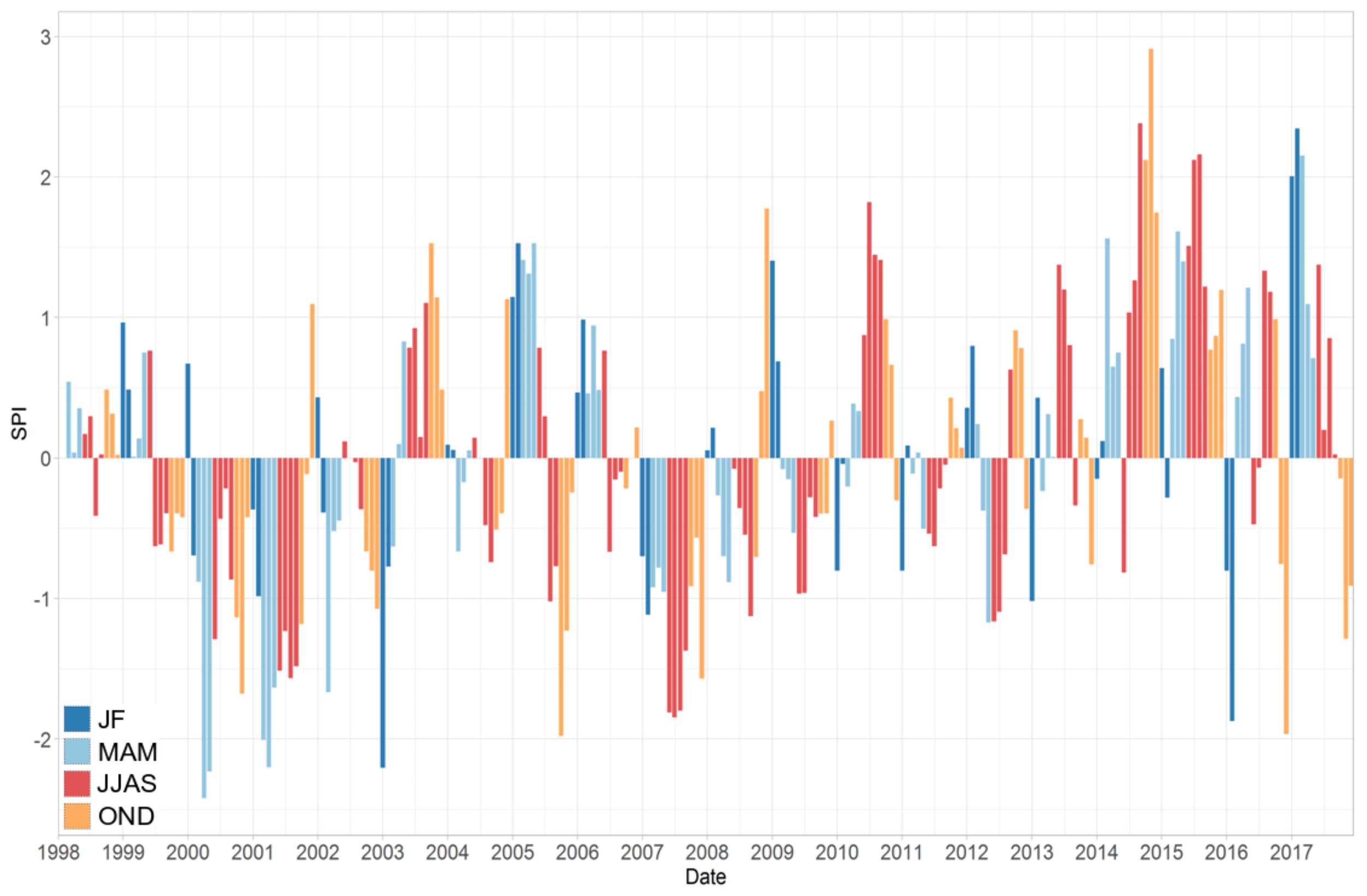
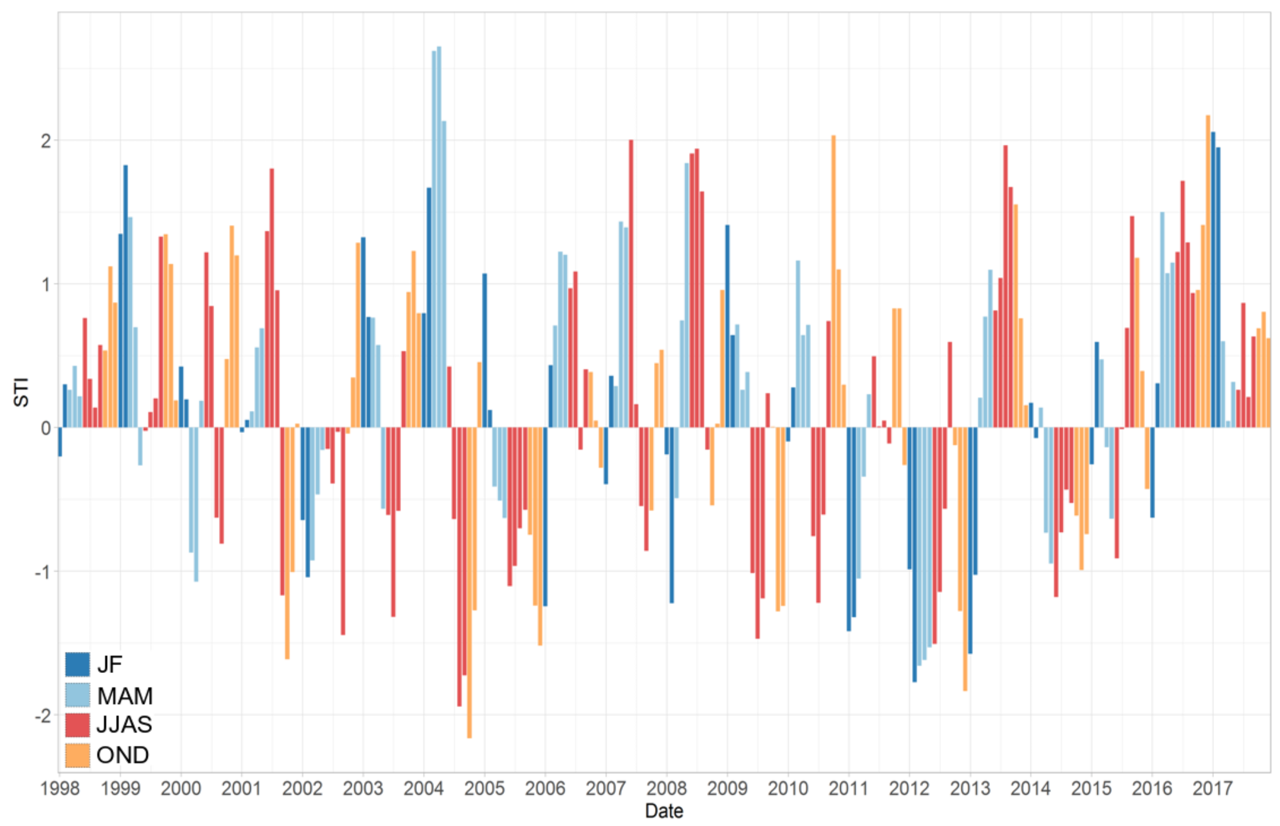
The mass balance and thus also the ice flux of Baltoro Glacier are influenced by melt and snow precipitation, which particularly deposits on high-elevation basins and slopes and redistributes by wind into the firn fields, or reaches the glacier via avalanches [7,35]. The supraglacial lakes arise if precipitation or melt water accumulates in depressions of the debris cover. Thus, both precipitation and melt are a potential driver of higher glacier velocities and evolution of supraglacial lakes. Therefore, the SPI index which is an indicator for precipitation surpluses and deficits (droughts) is analyzed for the period 1998 until 2017 (Figure 7). The color scheme in Figure 8 indicates the seasonal distribution in January and February (JF), from March to May (MAM), from June to September (JJAS), and from October to December (OND). The SPI index shows that the years 2006, 2008, 2010, 2014, 2015, and 2017 with a higher surface velocity are affected by higher winter precipitation. The years 2002, 2004, 2012, 2014, 2015, 2016, and 2017 with a higher number of supraglacial lakes are influenced by higher spring and early summer precipitation. Furthermore, for the period 1998–2014, a 3–4 year cycle in the amounts of precipitation can be recognized, whereas wet conditions persisted from 2014 to 2017. A positive correlation exists between precipitation and surface velocity as well as between precipitation and formation of supraglacial lakes. However, there are exceptions: in 2008, we identified an increase of supraglacial lakes despite normal precipitation (SPI index −0.1–−1.1). Hence, a general statement on which amount of precipitation over a specific period is required to provoke a certain surface velocity or number of supraglacial lakes, cannot be made. Additionally, the STI index as an indicator for temperature anomaly is analyzed for the period 1998 until 2017 (Figure 8). The color scheme in Figure 8 is adapted to Figure 7. For the periods with higher and lower glacier velocities, a clear trend is not visible. The years 2002, 2012, 2014, and 2015 with a higher number of supraglacial lakes are characterized by a cold early melt season (April to June), whereas the years 2004, 2013, 2016, and 2017 by a warm early melt season. Our data show a weak relationship between temperature and evolution of lakes, which is only visible in 2004, 2013, 2016, and 2017. Nevertheless, the SPI index shows a continuous warm period between August 2015 and December 2017. For a better readability, the SPI and STI indexes for the periods with divergent glacier velocities and supraglacial are listed in

Table 5. SPI and STI indexes divided into phases with higher and lower glacier velocities and into fewer and more supraglacial lakes.

	Date	SPI Index	STI Index
Periods with higher glacier velocity	01.12.2004–01.05.2005	1.1–1.5	−0.6–1.1
	01.01.2006–31.05.2006	0.5–1.0	−1.2–1.2
	01.02.2008–29.02.2008	0.2	−1.2
	01.11.2008–28.02.2009	0.5–1.8	0–1.4
	01.04.2010–31.05.2010	0.3–0.4	0.6–0.7
	01.10.2014–31.03.2015	0.6–2.9	−1.0–0.6
	01.10.2015–31.12.2015	0.8–1.2	−0.4–1.1
	01.01.2017–31.05.2017	0.7–2.3	0–2.0
Periods with lower glacier velocity	01.12.2012–31.01.2013	−0.4–−1.0	−1.8–1.6
	01.12.2013–31.01.2014	0.1–−0.8	0.1–0.2
Periods with more supraglacial lakes	01.06.2002–31.07.2002	0.1–0.0	−0.1–−0.4
	01.05.2004–31.07.2004	0.2–0.1	−0.6–2.1
	01.03.2008–30.09.2008	−0.1–−1.1	−0.5–1.9
	01.03.2012–31.03.2012	1.7	0.2
	01.04.2013–30.09.2013	0.3–1.4	0.7–1.9
	01.03.2014–30.09.2014	0.6–2.4	−1.1–0.1
	01.04.2015–30.09.2015	0.9–2.1	−0.9–1.5
	01.04.2016–30.09.2016	0.4–1.3	0.9–1.7
	01.04.2017–31.08.2017	2.1–1.4	0–0.8
Periods with fewer supraglacial lakes	01.06.2000–31.09.2000	−0.2–−1.3	−0.8–1.2
	01.06.2001–31.09.2001	−1.2–−1.6	0.9–1.8
	01.06.2009–31.09.2009	−0.2–−1.0	−1.5–0.2
	01.06.2011–31.09.2011	−0.0–−0.6	−0.1–0.5

.

6. Discussion

6.1. Surface Velocity

The SAR data cover a considerably long period from 1993 to 2017. However, in the early 1990s and 2000s, no continuous data acquisition was carried out and thus only snapshots for glacier conditions are available. Since 2014, Sentinel-1A has has provided continuous global monitoring with a temporal resolution of 12 days and a complete coverage of mountain glaciers worldwide, including Baltoro Glacier. After the launch of Sentinel-1B, Baltoro Glacier has been mapped every 12 days since 2017. Hence, the time series is inhomogeneous regarding the number of acquisitions and acquisition dates, which has to be considered for the comparison between different years. We identify a cyclical variability of the averaged summer surface velocity of the Baltoro Glacier with velocity lows in 2010, 2013, and 2014 and velocity highs in 2005, 2006, 2009, and 2015. Since 2015, the spatial pattern of the summer surface velocity has changed: in 2005 and 2006, the high surface velocities are concentrated between Concordia and Gore, whereas after 2015 the glacier acceleration extends further downstream to Urdukas (10 km). This phenomenon may be linked to the increasing formation of lakes, especially in the upstream part, which is explained in more detail in Section 6.3.

Some previous studies are based on different time periods or scientific foci, for example, [8,10], which hampers a direct comparability with our study. Quincey et al. [9] calculated annual surface velocities for 1993–2008, summer velocities for 1996–2005, and winter velocities for 1997–2006 based on ERS-1/2 and Envisat ASAR images. The comparison of annual surface velocities for the period 2004–2006 with our results showed only minor differences, which are most likely due to the usage of different glacier centerlines, coordinates for the terminus, and tracking patch sizes. Our summer velocities of 2005 are generally lower compared to Quincey et al. [9], due to a different length of the observation period and our approach to average multiple velocity fields to a single velocity field. However, Quincey et al. [9] proposed that high surface velocities during summer 2005 were induced by a peak of precipitation in the previous winter, which is consistent with our findings. For the period 2006–2008, Quincey et al. [9] reported a velocity decrease. Though, in our case, the summer velocities from 2006 to 2008 had higher rates, as we used additional ALOS PALSAR-1 data from 2007 and 2008 covering the time period with higher surface velocities. Sun et al. [3] analyzed the annual velocities over the central Karakoram for the period 1999–2003 using Landsat-7 ETM+ imagery and for the period 2007–2011, whereas the latter period has also been investigated by Rankl et al. [10]. Sun et al. [3] observed a 50% higher average velocity between 2007 and 2011 in comparison to the period 1999–2003, whereas Quincey et al. observed a speed-up of 15–20% from 2006 to 2008 [9]. Hence, Sun et al. [3] suggested a slight speed-up of the glacier from 2008 to 2011. This conclusion agrees with our observed glacier acceleration in 2008 and 2009. For 2010–2011, we only had two SAR acquisitions available (14 May 2010 and 23 May 2010), which restricts further investigations about the nature and duration of this speed-up. Usman and Furuya [11] investigated the spatio-temporal velocity variability based on ALOS PALSAR-1/2 data, acquired in the periods 2007–2011 and 2014–2015. They found a speed-up in 2008, a slowdown between 2009 and 2010, and an overall speed-up between 35 and 25 km distance from the terminus in 2015. The last displacement result bases on ALOS PALSAR-2 data, which covers only the upstream part of the glacier. Due to different acquisition orbits, just a single acquisition is required to cover the whole Baltoro Glacier with ALOS PALSAR-1 data, whereas with ALOS PALSAR-2 data, at least four acquisitions are needed to ensure a full coverage of the glacier. Nevertheless, their results confirm our observed glacier acceleration in 2008 and 2009, as well as the higher displacement between Concordia and Gore in 2015. Previous studies focused only on single events and short time series. Our study, based on a continuous, long-term time series from 1992–2017, is the first to enable an investigation of the detailed magnitude and timing of the summer speed-up events and to confirm that the events underlie a 3–4-year cycle.

6.2. Supraglacial Lakes

The lakes undergo a 3–4-year cycle, which varies between phases with fewer than 200 lakes and a total lake area of less than 1.4 km² and phases with more than 200 lakes and a lake area of 1.4–1.9 km². In 2014, 2016, and 2017, the total lake area was significantly larger than 2.0 km². The increasing formation of supraglacial lakes correlates with the high amount of precipitation in spring and early summer. Both, the supraglacial lakes and the precipitation reflect the 3–4 year cycle and the large increase since 2012. Due to the absence of snow on the glacier surface during summer, only Landsat and ASTER data acquired between June and August were used. Hence, the annual comparisons may be biased by different acquisition dates. The classification results of the years with two optical satellite acquisitions show a high variability within one season and prove that most of the lakes disappear, but a few lakes arise or even persist during the summer season. Using images acquired at exactly the same time of year or a denser time series in order to better reflect the variability within one season and between years is unfortunately not possible due to low data inventory, cloud coverage, and missing data (e.g., failure of the Scan Line Corrector of Landsat-7).

Veettil et al. [36] mapped the lakes from four images acquired in July 1978 (1.145 km²), July 1993 (1.948 km²), June 2002 (2.395 km²), and June 2014 (2.164 km²) based on Landsat imagery. They observed an increase of lakes from the late 1970s towards the late 2000s and a stable state between 2002 and 2014. Furthermore, they identified a connection between the increase of lakes and the Pacific Decadal Oscillation (PDO) and El Niño-Southern Oscillation (ENSO), respectively. The formation and the expansion of the lakes occur during the warm regime of PDO, particularly during the wet conditions between January and April affected by El Niño [36]. Unfortunately, the large increase of lakes from 2012 to 2017 invalidate their assumption: 2014/2015 and 2015/2016 were affected by the wet conditions of El Niño, whereas 2011/2012 and 2016/2017 were influenced by the dry conditions of La Niña [37]. Gibson et al. [38] analyzed the supraglacial lakes between 2001 and 2012 based on three images acquired in 29 August 2001 (0.66 km²), 14 August 2004 (1.79 km²), and 20 August 2012 (2.04 km²), observing an increasing number of lakes between 2001 and 2012 and particularly between 2001 and 2004, which can be attributed to changes in precipitation since 2000 [38]. Our results differ by ±0.5 km² from the results of Veettil et al. [36] and ±0.2 km² at maximum from Gibson et al. [38]. The differences can be explained by the usage of different thresholds and spectral bands. Yet, the former studies are based on multiple timestamps with only one image every 3–9 years. A low amount of data does not allow to describe the annual or seasonal variability and can lead to a misinterpretation of the lake behavior. Our study is based on all available optical data of Landsat and ASTER in order to support a dense time series and hence to analyze, describe, and understand better the high variability of the supraglacial lakes.

6.3. Relationship between Summer Surface Velocities, Supraglacial Lakes, and Climate

The analysis of the SPI index indicates a linkage between precipitation and surface velocity: heavy winter precipitation evokes glacier acceleration in summer. Quincey et al. [9] have already stated the direct relationship between winter precipitation and summer velocity for the period 1993–2008. Hence, our study confirms their observation for a longer time period. The winter precipitation particularly accumulates in the high elevation basins and steep valley slopes as snow and redistributes by wind into the firn field or reaches the glacier via avalanches. Both deposition mechanisms are the main source of mass for the formation and hence of the higher summer surface velocities. For the period 1998–2014, the winter precipitation is characterized by a duration of a few months only, with a moderate total amount (SPI between +1.0 and +1.5). From 2014 to 2017, the winter precipitation changed: (1) it persists longer, (2) it starts as early as fall, and (3) it shows a larger intensity (4 months with an SPI index >+2.0).

Additionally, the SPI index shows a connection between precipitation and evolution of supraglacial lakes: a higher spring and early summer precipitation might be responsible for an increase of supraglacial lake number and area, as precipitation—rainfall or snow melt—accumulates in the depressions of the hummocky and debris-covered surface topography of the lower part of the glacier. The upper part has a smoother surface with fewer depressions and existing drainage channels, which supports a fast water run-off and thus a less likely generation of ponds. However, the area on which lakes arise has enlarged: Until 2012, most of the lakes developed between the glacier termini and the confluence of Yermanendu Glacier (20 km), whereas from 2014 to 2017, the area between the glacier terminus and the confluence of Biarchedi Glacier (30 km) was affected. This change has an impact on the surface velocity. In 2005, 2006, and 2009, the glacier had its highest surface velocities only in the upper part between Concordia and Gore. However, in 2015, 2016, and 2017, we identified higher surface velocities between Concordia and Urdukas as well. We hypothesize that the higher availability of surface water stored in the lakes enables increased basal sliding, if the water is able to drain from the lakes through the glacier. The higher velocities very likely lead to increased crevassing. Though this cannot be detected in our remote sensing imagery due to coarse spatial resolution, this phenomenon has already been observed in several studies [39,40,41]. Therefore, we hypothesize that the increase of cracks and crevasses enable a more intense deep drainage of the melt water towards the glacier base. The surface velocity increase during early melt season due to subglacial drainage systems followed by a late summer slow-down with a mature subglacial drainage system has been already observed for example on glaciers in Greenland, the Alps, and Pamir [42,43,44,45]. The STI index offers no influence of the temperatures on the evolution of the supraglacial lakes. Though, for the years 2015–2017 a warmer melting seasons is observed, which probably induced a higher number of lakes during that time and raised the amount of melt water.

Table 6. Chronological process of surface velocities, supraglacial lakes, and precipitation.

	Beginning	Event
1.Phase	January/February	strong winter precipitation
	End of May/Mid of June	initial glacier acceleration
2.Phase	May/June	strong spring and summer precipitation
		formation of supraglacial lakes
3.Phase	Begin/Mid of June	formation of crevasses due to first glacier acceleration
		drainage of lake water through crevasses off to the ground
		forcing basal sliding for the lower part of the glacier
		continuing glacier acceleration

summarizes the process. It should be noted that the events mostly occur in parallel, so an exact termination is not possible.

Why did more lakes develop between 2014 and 2017 extending more than 10 km further up-glacier than before? Increasing supraglacial lakes lead to a surface lowering [38]. If the lake water warms up by incoming solar radiation, this energy will be used for melting and the extension of the small depressions, leading to an undulated topography. This in turn promotes, in case of higher precipitation as well as increased melting, the formation of supraglacial lakes [38,46,47]. Dobreva et al. [1] reported that, during their fieldwork in July 2005, the glacier surface topography changed rapidly within a week due to the ice dynamics induced by sediment fluxes, supraglacial fluvial processes, and the evolution of supraglacial lakes and ice cliffs. Unfortunately, we have no information about the supraglacial lakes in 2005 due to missing Landsat and ASTER data. However, the high SPI index of 0.3–1.5 from 1 March 2005 to 31 July 2005 (Figure 7) suggests an increase of supraglacial lakes, which confirms their observation. Due to the large total area of supraglacial lakes and thereby the absorption of solar radiation, we presume a warming of the air temperature and a transformation of a smooth to a hummocky surface in the 10 km further up-glacier. Additionally, the long and continuous precipitation period from 2014 to 2017 with a high SPI index of >+1.0 indicates an intensification of the westerlies and the Indian summer monsoon.

7. Conclusions

The dense time series of available SAR data acquired by ERS-1/2, Envisat ASAR, ALOS PALSAR-1, TerraSAR-X, TanDEM-X, and Sentinel-1 are used to analyze the annual and (intra-)seasonal surface velocity evolution of Baltoro Glacier from 1992 to 2017. As basal sliding, controlled by seasonal water supply at the glacier base, dominates the ice flow, we investigate the potential correlation between glacier surface velocity, the occurrence of supraglacial lakes, seasonal precipitation intensity, and temperature. We mapped the total number and area of supraglacial lakes from multi-spectral Landsat and ASTER imagery and evaluated the precipitation data from TRMM for the same period. Our study shows that the surface velocity of Baltoro Glacier underlies a 2–7 year cycle with summer speed-ups in 2005, 2006, 2008, and 2010 and persistent high velocities from 2015 to 2017. In addition, we show that the supraglacial lake evolution underlies a 3–4 year cycle, with a total lake area of more than 1.4 km² in 1991, 1993, 2002, 2004, and 2008, but continuously large lake areas in the ablation seasons of 2012 to 2017. Both, the velocity speed-ups and the supraglacial lakes area fluctuations are influenced by the precipitation intensity: high winter precipitation is very likely linked to glacier speed-ups starting from end of May to early June, whereas heavy spring and early summer precipitation induces an increase of supraglacial lakes at the beginning of June. In only a few years, the higher temperatures during the early melt season additionally influenced the evolution of lakes and hence the raise of melt water on the glacier. However, the continuous warm period from 2015 to 2017 effectuated the increase of surface velocities between Gore and terminus and the higher number of lakes between the confluence of Yermanendu and Biarchedi Glacier (20–30 km). We postulate that higher amounts of water stored in the supraglacial lakes caused increased basal sliding and thus an additional mobilization of the glacier between Gore and Urdukas. The initial glacier acceleration induced by the increased winter precipitation led to more crevasses, which acted as pathways for the drainage of lake water (e.g., through hydro-fracturing) and enhanced the basal sliding. The increase in supraglacial lakes changed the spatial pattern of surface velocity: during the summer speed-ups in 2005, 2006, and 2009, higher velocities were concentrated between Concordia and Gore, whereas in 2015 the glacier acceleration affected the glacier between Concordia and downstream to Urdukas. Furthermore, in 2015, 2016, and 2017, the acceleration of the Trango Glacier influenced the surface velocity of the Baltoro Glacier. It is likely that, after the acceleration, the Trango Glacier stretched the Baltoro Glacier and thus induced the generation of crevasses on the Baltoro Glacier. This again provoked the drainage of the supraglacial lakes upwards of the tributary and led to a steeper velocity gradient near the terminus (10–5 km).

Due to the complex nature of glaciers, only the consideration of all major influencing factors such as precipitation, glacial characteristics, and their connection allows for an understanding of the glacier behavior and its dynamics. However, a long-term and continuous time series over 2 or 3 decades enables the analysis of annual and (intra-)seasonal processes as well as the determination of magnitude and timing of short-term events - dependent on the availability and acquisition date of remote sensing data. There is no simple relationship between precipitation, glacier dynamics, and supraglacial lakes that would allow one to derive the amount of precipitation needed to produce a higher summer speed-up or a larger increase of lake numbers and area. Moreover, in some years a summer speed-up occur despite a low winter precipitation (e.g., 2008). Nevertheless, an intensification of both precipitation and the formation of supraglacial lakes is clearly recognizable, which changed the ice dynamic of the Baltoro Glacier considerably in recent years.

References

- Dobreva, I.D.; Bishop, M.P.; Bush, A.B.G. Climate–Glacier Dynamics and Topographic Forcing in the Karakoram Himalaya: Concepts, Issues and Research Directions. Water 2017, 9, 405. [Google Scholar] [CrossRef]
- Shroder, J.F.; Bishop, M.P. Glaciers of Pakistan. In Satellite Image Atlas of Glaciers of the World: Asia; Professional Paper 1386-F; US Government Printing Office: Washington, DC, USA, 2010; pp. 201–257. [Google Scholar]
- Sun, Y.; Jiang, L.; Liu, L.; Sun, Y.; Wang, H. Spatial-Temporal Characteristics of Glacier Velocity in the Central Karakoram Revealed with 1999–2003 Landsat-7 ETM+ Pan Images. Remote Sens. 2017, 9, 1064. [Google Scholar] [CrossRef]
- Kaser, G.; Großhauser, M.; Marzeion, B. Contribution potential of glaciers to water availability in different climate regimes. Proc. Natl. Acad. Sci. USA 2010, 107, 20223–20227. [Google Scholar] [CrossRef] [PubMed]
- Bolch, T.; Kulkarni, A.; Kääb, A.; Huggel, C.; Paul, F.; Cogley, J.; Frey, H.; Kargel, J.S.; Fujita, K.; Scheel, M. The State and Fate of Himalayan Glaciers. Science 2012, 336, 310–314. [Google Scholar] [CrossRef] [PubMed] [Green Version]
- Huss, M.; Hock, R. Global-scale hydrological response to future glacier mass loss. Nat. Clim. Chang. 2018, 8, 135–140. [Google Scholar] [CrossRef] [Green Version]
- Mayer, C.; Lambrecht, A.; Belo, M.; Smiraglia, C.; Diolaiutt, G. Glaciological characteristics of the ablation zone of Baltoro glacier, Karakoram, Pakistan. Ann. Glaciol. 2006, 43, 123–131. [Google Scholar] [CrossRef]
- Copland, L.; Pope, S.; Bishop, M.P.; Shroder, J.F.; Clendon, P.; Bush, A.; Kamp, U.; Seong, Y.B.; Owem, L.A. Glacier velocities across the central Karakoram. Ann. Glaciol. 2009, 50, 41–49. [Google Scholar] [CrossRef]
- Quincey, D.J.; Copland, L.; Mayer, C.; Bishop, M.; Luckman, A.; Belò, M. Ice velocity and climate variations for Baltoro Glacier, Pakistan. J. Glaciol. 2009, 55, 1061–1071. [Google Scholar] [CrossRef]
- Rankl, M.; Kienholz, C.; Braun, M. Glacier changes in the Karakoram region mapped by multimission satellite imagery. Cryosphere 2014, 8, 977–989. [Google Scholar] [CrossRef] [Green Version]
- Usman, M.; Furuya, M. Interannual modulation of seasonal glacial velocity variations in the Eastern Karakoram detected by ALOS-1/2 data. J. Glaciol. 2018, 64, 465–476. [Google Scholar] [CrossRef] [Green Version]
- Greenbelt, M.D. Tropical Rainfall Measuring Mission (TRMM), TRMM (TMPA/3B43) Rainfall Estimate L3 1 Month 0.25 Degree x 0.25 Degree V7; Goddard Earth Sciences Data and Information Services Center (GES DISC): Greenbelt, MD, USA, 2011. [Google Scholar]
- Dee, D.P.; Uppala, S.M.; Simmons, A.J.; Berrisford, P.; Poli, P.; Kobayashi, S.; Andrea, U.; Balmaseda, M.A.; Balsamo, G.; Bauer, P.; et al. The ERA-Interim reanalysis: Configuration and performance of the data assimilation system. Q. J. R. Meteorol. Soc. 2011, 137, 553–597. [Google Scholar] [CrossRef]
- Mihalcea, C.; Mayer, C.; Diolaiutt, G.; D’Agata, C.; Smiraglia, C.; Lambrecht, A.; Vuillermoz, E.; Tartari, G. Spatial distribution of debris thickness and melting from remote-sensing and meteorological data, at debris-covered Baltoro glacier, Karakoram, Pakistan. Ann. Glaciol. 2008, 48, 49–57. [Google Scholar] [CrossRef]
- Kraaijenbrink, P.D.A.; Bierkens, M.F.P.; Lutz, A.F.; Immerzeel, W.W. Impact of a global temperature rise of 1.5 degrees Celsius on Asia’s glaciers. Nature 2017, 549, 257–263. [Google Scholar] [CrossRef] [PubMed]
- Evatt, G.W.; Mayer, C.; Mallinson, A.; Abrahams, I.D.; Heil, M.; Nicholson, L. The secret life of ice sails. J. Glaciol. 2017, 63, 1049–1062. [Google Scholar] [CrossRef]
- Juen, M.; Mayer, C.; Lambrecht, A.; Han, H.; Liu, S. Impact of varying debris cover thickness on ablation: A case study for Koxkar Glacier in the Tien Shan. Cryosphere 2014, 8, 377–386. [Google Scholar] [CrossRef] [Green Version]
- Hobbs, W.H. Characteristic of Existing Glaciers; Macmillan: New York, NY, USA, 1922. [Google Scholar]
- Strozzi, T.; Luckman, A.; Murray, T.; Wegmuller, U.; Werner, C.L. Glacier motion estimation using SAR offset-tracking procedures. IEEE Trans. Geosci. Remote Sens. 2002, 40, 2384–2391. [Google Scholar] [CrossRef] [Green Version]
- Dehecq, A.; Gourmelen, N.; Trouve, E. Deriving large-scale glacier velocities from a complete satellite archive: Application to the Pamir–Karakoram–Himalaya. Remote Sens. Environ. 2015, 162, 55–66. [Google Scholar] [CrossRef] [Green Version]
- Lüttig, C.; Neckel, N.; Humbert, A. A Combined Approach for Filtering Ice Surface Velocity Fields Derived from Remote Sensing Methods. Remote Sens. 2017, 9, 1062. [Google Scholar] [CrossRef]
- Friedl, P.; Seehaus, T.C.; Wendt, A.; Braun, M.H.; Höppner, K. Recent dynamic changes on Fleming Glacier after the disintegration of Wordie Ice Shelf, Antarctic Peninsula. Cryosphere 2018, 12, 1347–1365. [Google Scholar] [CrossRef]
- McFeeters, S.K. The use of Normalized Difference Water Index (NDWI) in the delineation of open water features. Int. J. Remote Sens. 1996, 17, 1425–1432. [Google Scholar] [CrossRef]
- Wessels, R.L.; Kargel, J.S.; Kieffer, H.H. ASTER measurement of supraglacial lakes in the Mount Everest region of the Himalaya. Ann. Glaciol. 2002, 34, 399–408. [Google Scholar] [CrossRef]
- Bolch, T.; Buchroithner, M.F.; Peters, J.; Baessler, M.; Bajracharya, S. Identification of glacier motion and potentially dangerous glacial lakes in the Mt. Everest region/Nepal using spaceborne imagery. Nat. Hazards Earth Syst. Sci. 2008, 8, 1329–1340. [Google Scholar] [CrossRef] [Green Version]
- Gao, B. NDWI—A normalized difference water index for remote sensing of vegetation liquid water from space. Remote Sens. Environ. 1996, 58, 257–266. [Google Scholar] [CrossRef]
- Xu, H. Modification of normalised difference water index (NDWI) to enhance open water features in remotely sensed imagery. Int. J. Remote Sens. 2006, 27, 3025–3033. [Google Scholar] [CrossRef]
- Lacaux, J.; Tourre, Y.; Vignolles, C.; Ndione, J.; Lafaye, M. Classification of ponds from high-spatial resolution remote sensing: Application to Rift Valley Fever epidemics in Senegal. Remote Sens. Environ. 2007, 106, 66–74. [Google Scholar] [CrossRef]
- McKee, T.B.; Doesken, N.J.; Kleist, J. The relationship of drought frequency and duration to time scales. In Proceedings of the 8th Conference on Applied Climatology, Anaheim, CA, USA, 17–22 January 1993; Volume 17, pp. 179–183. [Google Scholar]
- Svoboda, M.; Hayes, M.; Wood, D. Standardized Precipitation Index User Guide; WMO-No. 1090; World Meteorological Organization: Geneva, Switzerland, 2012; pp. 399–408. [Google Scholar]
- Edwards, D.C.; McKee, T.B. Characteristics of 20th century drought in the United States at multiple time scales. Climatol. Rep. 1997, 97, 1049–1062. [Google Scholar]
- Shah, R.; Mishra, V. Evaluation of the Reanalysis Products for the Monsoon Season Droughts in India. J. Hydrometeorol. 2014, 15, 1575–1591. [Google Scholar] [CrossRef]
- Schöne, B.R. A ‘clam-ring’ master-chronology constructed from a short-lived bivalve mollusc from the northern Gulf of California, USA. Holocene 2003, 13, 39–49. [Google Scholar] [CrossRef]
- Winkler, K.; Gessner, U.; Hochschild, V. Identifying Droughts Affecting Agriculture in Africa Based on Remote Sensing Time Series between 2000–2016: Rainfall Anomalies and Vegetation Condition in the Context of ENSO. Remote Sens. 2017, 9, 831. [Google Scholar] [CrossRef]
- Von Wissmann, H. Die heutige Vergletscherung und Schneegrenze in Hochasien. Akad. Wiss. Lit. Mainz Abh. Math.-Naturw. Kl. 1959, 14, 1101–1407. [Google Scholar]
- Veettil, B.K.; Bianchini, N.; Bremer, U.F.; Maier, E.L.B.; Simões, J.C. Recent variations of supraglacial lakes on the Baltoro Glacier in the central Karakoram Himalaya and its possible teleconnections with the pacific decadal oscillation. Geocarto Int. 2016, 31, 109–119. [Google Scholar] [CrossRef]
- NOAA—National Oceanic and Atmospheric Administration. National Weather Service. 2018. Available online: http://origin.cpc.ncep.noaa.gov/products/analysismonitoring/ensostuff/ONIv5.php (accessed on 30 August 2018).
- Gibson, M.J.; Glasser, N.F.; Quincey, D.J.; Mayer, C.; Rowan, A.V.; Irvine-Fynna, T.D.L. Temporal variations in supraglacial debris distribution on Baltoro Glacier, Karakoram between 2001 and 2012. Geomorphology 2017, 295, 572–585. [Google Scholar] [CrossRef]
- Copland, L.; Sharp, M.J.; Nienow, P.W. Links between short-term velocity variations and the subglacial hydrology of a predominantly cold polythermal glacier. J. Glaciol. 2003, 49, 337–348. [Google Scholar] [CrossRef]
- Benn, D.; Gulley, J.; Luckman, A.; Adamek, A.; Glowacki, P.S. Englacial drainage systems formed by hydrologically driven crevasse propagation. J. Glaciol. 2009, 55, 513–523. [Google Scholar] [CrossRef]
- Gong, Y.; Zwinger, T.; Åström, J.; Altena, B.; Schellenberger, T.; Gladstone, R.; Moore, J.C. Simulating the roles of crevasse routing of surface water and basal friction on the surge evolution of Basin 3, Austfonna ice cap. Cryosphere 2018, 12, 1563–1577. [Google Scholar] [CrossRef] [Green Version]
- Joughin, I.; Smith, E.; Howat, I.M.; Floricioiu, D.; Alley, R.B.; Truffer, M.; Fahnestock, M. Seasonal to decadal scale variations in the surface velocity of Jakobshavn Isbræ, Greenland: Observation and model-based analysis. J. Geophys. Res. 2012, 117, 1–20. [Google Scholar] [CrossRef]
- Anderson, R.S.; Anderson, S.P.; MacGregor, K.R.; Waddington, E.D.; O’Neel, S.; Riihimaki, C.A.; Loso, M.G. Strong feedbacks between hydrology and sliding of a small alpine glacier. J. Geophys. Res. 2004, 109, 1–17. [Google Scholar] [CrossRef]
- Bevana, L.S.; Luckmana, A.; A.Khan, S.; Murraya, T. Seasonal dynamic thinning at Helheim Glacier. Earth Planet. Sci. Lett. 2015, 415, 47–53. [Google Scholar] [CrossRef] [Green Version]
- Lambrecht, A.; Mayer, C.; Aizen, V.; Floricioiu, D.; Surazakov, A. The evolution of Fedchenko glacier in the Pamir, Tajikistan, during the past eight decades. J. Glaciol. 2014, 60, 233–244. [Google Scholar] [CrossRef] [Green Version]
- Sakai, A.; Takeuchi, N.; Fujita, K.; Nakawo, M. Role of supraglacial ponds in the ablation process of a debris-covered glacier in the Nepal Himalayas. In Debris-Covered Glaciers, Proceedings of an International Workshop, Seattle, WA, USA, 2000; Volume 264, pp. 119–132.
- Leeson, A.A.; Shepherd, A.; Briggs, K.; Howat, I.; Fettweis, X.; Morlighem, M.; Rignot, E. Supraglacial lakes on the Greenland ice sheet advance inland under warming climate. Nat. Clim. Chang. 2015, 5, 51–55. [Google Scholar] [CrossRef]
Figure 1.
Overview of Baltoro Glacier, Pakistan, with the glacier boundaries (blue) and the glacier centerline (red). The background image is a Landsat-7 scene acquired on 12 July 2010, which has been also used for derivation of the glacier boundaries based on the Normalized Difference Snow index (NDSI) and manual editing.
Figure 2.
Annual surface velocities (m a−1) along the glacier centerline.
Figure 3.
Averaged summer surface velocities (m a−1) along the glacier’s centerline.
Figure 4.
Averaged winter surface velocities (m a−1) along the glacier’s centerline.
Figure 5.
Heatmap of summer surface velocities (m a−1) from May to September along the glacier centerline for 1999–2017.
Figure 6.
Heatmap of winter surface velocities (m a−1) from October to April along the glacier centerline.
Figure 7.
SPI from 1998 to 2017 for the monthly precipitation intensity, color-coded for the seasonal distribution: January and February (JF) in dark blue, March to May (MAM) in light blue, June to September (JJAS) in red, and October to December (OND) in orange.
Figure 8.
STI from 1998 to 2017 for the monthly temperature anomaly, color-coded for the seasonal distribution: January and February (JF) in dark blue, March to May (MAM) in light blue, June to September (JJAS) in red, and October to December (OND) in orange.