Seasonality of the Physical and Biogeochemical Hydrography in the Inflow to the Arctic Ocean Through Fram Strait

1. Introduction

The rapid environmental changes occuring in the Arctic Ocean in recent decades include a process in the Atlantic sector sometimes referred to as “Atlantification.” Although it is currently not entirely clear whether this strengthened inflow of water from the North Atlantic is due to a climatic cycle, with data commonly going back to at most the late 1990s (e.g., Årthun et al., 2012; Polyakov et al., 2017), it is sometimes taken to express a fundamental shift of the Arctic Arctic to a new marine climate (Polyakov et al., 2017). In essence, “Atlantification” entails a replacement of water masses formed and advected from the central Arctic by water of Atlantic origin (Årthun et al., 2012), flowing northward along the shelf slope (West Spitsbergen Current, Fram Strait Branch) as a boundary current, and through the Barents Sea (Barents Sea Branch), later joining the Fram Strait Branch at St. Anna Trough. Because the highly saline Atlantic Water (AW) is temperature-stratified, its weak water column stability is easily overcome by thermal convection. As opposed to the permanently salt-stratified central Arctic, this allows for efficient replenishment of upper-ocean nutrients early in winter over the shelf slope (Randelhoff et al., 2015). The release of large amounts of heat during winter exerts a strong control on the location of the ice edge (Untersteiner, 1988). This sea ice is usually advected from the Kara Sea (Pfirman et al., 1997), rather than formed locally. Reports of increasing AW temperatures throughout the Arctic (Polyakov et al., 2012) suggest that this heat has probably driven the bulk of the sea ice loss north of Svalbard in recent decades (Onarheim et al., 2014). When sea ice comes close to the heat stored in the AW, it melts and forms a near-surface layer of fresh, cold water, a crucial ingredient that shapes the planktonic ecosystem bustling and blooming in the summer months. One immediate implication is that near-surface AW penetrating further and further east has the capability to relieve both nutrient and light limitation on the shelf slope north-east of Svalbard, leading to increased productivity. Indeed, Slagstad et al. (2015) project that in the northern Barents and Kara seas, primary production might increase locally by up to 40–80 g C m⁻² year⁻¹ by 2,100.

Winter is traditionally undersampled in the Arctic Ocean. Only recently has the extreme loss of winter sea ice north of Svalbard mentioned above enabled research vessels to easily visit the area in the depth of winter, leading to new insights such as on ecosystem functioning during the longer polar night (Berge et al., 2015). Given the control Atlantic Water exerts on the heat (Rudels et al., 2015) and nutrient (Torres-Valdés et al., 2013) budgets of the Arctic Ocean, there is also the need for comprehensive and concurrent measurements of the key physical and biogeochemical elements in the AW inflow region. And even though the absence of light means no photosynthesis and thus no primary production, it is exactly in winter that the ecosystem is preconditioned for the next spring and summer, for example by setting up nutrient inventories. The Arctic ecosystem is therefore hinged on how these are modified through the annual cycle and as they travel from the Fram Strait and into the AO along the continental slope. In this study we summarize and discuss the key physical and biogeochemical changes occurring in the Fram Strait Atlantic Water inflow to the AO through a full annual cycle, and doing so form a basis for discussion and interpretation of the biological results obtained simultaneously during five field campaigns in 2014 and published in this special issue.

2. Data and Methods

2.1. Data Set

The data presented here were collected during five cruises in January, March, May, August and November 2014 west and north of Spitsbergen as part of the CarbonBridge and MicroPolar projects. We discuss a total of five transects across the AW core (January, May, August) and six 30-h process stations (May and August), where comprehensive sampling of the lower trophic level ecosystem in addition to biogeochemical and physical measurements were conducted. These observations are supplemented with observations of physical and biogeochemical parameters during March and November (sampled as part of the MicroPolar project) to increase temporal coverage and resolution of the region.

Parameters discussed in this study include:

• Conductivity-temperature-depth (CTD) profiles

• Inorganic nutrients: Nitrate+nitrite (${\text{NO}}_2^{-}$+${\text{NO}}_3^{2-}$), silicic acid (Si(OH)₄, often called silicate and abbreviated as silica, Si), phosphate (${\text{PO}}_4^{3-}$), and ammonium (${\text{NH}}_4^{+}$)

• Chlorophyll-a concentration

• Fugacity of CO₂ (fCO₂)

• Photosynthetically available radiation (PAR)

It was desirable to sample as far east and north as possible (downstream the AW flow and into the ice), but unusually heavy ice cover around Svalbard during much of 2014 only allowed repetition of one May process station in August. The following is an overview over all occupied stations described and analyzed in this study (for a more detailed overview, see Figure 1 and Table S1).

• Transect D (January, May and August): 79°N, 4–10°E

• Transect B (January): across the shelf slope north of Spitsbergen, approximately 20°E

• Process stations in May: P1, P3, P4

• Process stations in August: P5, P6, P7, where P6 and P7 were across the shelf slope north of Spitsbergen, approximately 15°E

• Supplemented by: One station north of Spitsbergen, March 2014, and three stations situated along the D transect in November 2014.

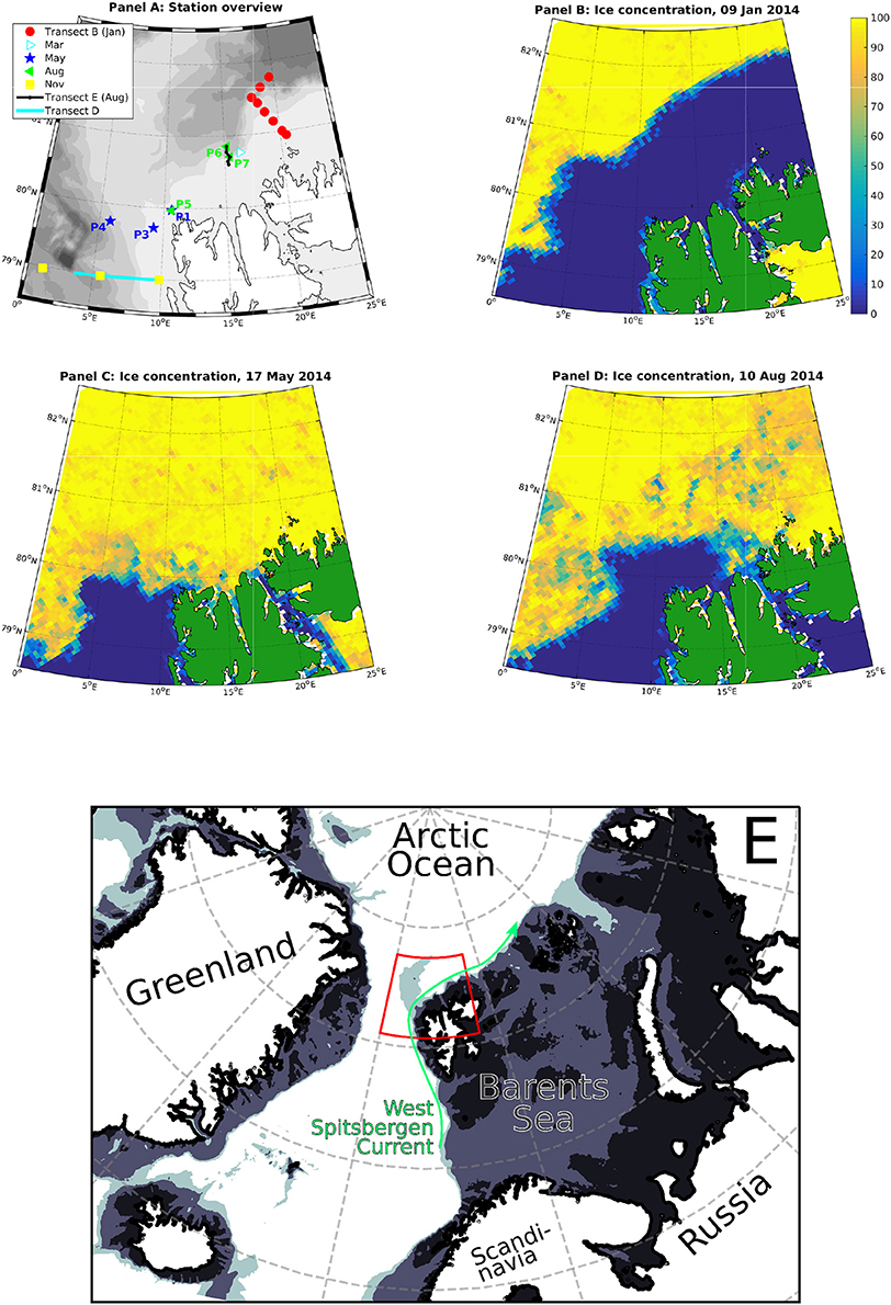
Figure 1. Map of the study area (A) in its larger geographic context (E; red outline: study area), and ice charts for the January, May and August cruises (B–D). Transect D was sampled in January, May, August and November. Every cruise featured some additional stations further north, in particular transect B in January and transect E in August (which includes P6 and P7). All stations sampled in March and November were ice-free.

2.2. CTD System

Water samples were collected from 8-L Niskin bottles mounted on a General Oceanics 12-bottle rosette equipped with a Conductivity-Temperature-Depth sensor system (CTD, Seabird SBE-911 plus), including a Seapoint Fluorometer. Water was collected at a total of 11–14 depths during the first CTD profiles at each station. Samples were taken from surface to 1,000 m depth (or limited by station depth), with highest resolution in the upper 100 m. Subsamples for biological and chemical characterization such as Chlorophyll a (Chl-a) and nutrients were taken. Chl-a fluorescence was used to determine the depth of the chl-a maximum for bottle samples, and calibrated afterwards using chl-a bottle samples. Bottle samples were also collected to check conductivity cell drift. Salinity errors were small, on the order of 0.01, which agreed with the post-cruise slope correction. No corrections beyond standard SeaBird data processing routines routines were deemed necessary.

2.3. Water Masses

Water masses have been classified as follows (see also Figure 2). Atlantic Water (AW) is defined by salinity S > 34.92 and T > 2°C, for straightforward comparison with other data sets from the Fram Strait area (Walczowski, 2013, and references therein). We further delineate cold Atlantic Water (cAW) with 0 < T < 2 °C and Intermediate Water (IW) T < 0 °C (as in de Steur et al., 2014), both with S > 34.9 as the second defining limit. To identify water in the upper part of the column with characteristics typical of water that has undergone freshening and cooling inside the Arctic Ocean, we define Arctic Water (ArW) as having density ρ_θ > 27.7 kg m⁻³ and S < 34.92 (or 34.9 when cooler than 2°C). It is important to note that not all water thus classified as ArW necessarily originates from the Arctic Ocean interior, but it has undergone similar modification processes and so deserves to be classified as such for easier comparison with earlier literature. Surface Water (SW) is delimited by density ρ_θ < 27.7 kg m⁻³ (as in Marnela et al., 2013) and S < 34.92 to allow warm near-surface AW to remain in its original water mass (Beszczynska-Möller et al., 2012).

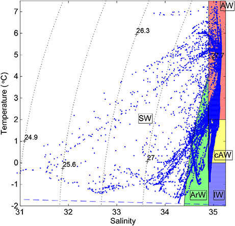
Figure 2. Temperature plotted against salinity based on the full-depth profiles from the onboard CTD system (see Section 2.2) including water mass definitions: Atlantic Water (AW), Cold Atlantic Water (cAW), Intermediate Water (IW), Arctic Water (ArW), and Surface Water (SW). For definitions in terms of temperature-salinity properties, see Section 2.3.

2.4. Sample Analysis and Data Processing

2.4.1. Calculation of Mixed-Layer Depth

For the purposes of this study, the depth of the mixed layer is defined as the depth where potential density (σ_θ) crosses 20% of the density difference between a surface layer density (3–5 m) and deeper (reference depth interval 50–60 m) values.

The reasoning behind this is that the upper ocean stratification observed during the summer cruises was often strong, yet shallow, not permitting the identification of a mixed layer in the classical sense of an actual well-mixed layer. Also note that whenever the density is homogeneous from the ocean surface to the bottom of the mixed layer, our algorithm gives results very similar to more standard methods, because all the density change happens in a rather thin pycnocline. Our method to study mixed layer depths was developed in more detail by Randelhoff et al. (2017).

Mixed layer depths were derived from CTD profiles measured by a MSS-90L microstructure sonde (ISW Wassermesstechnik, Germany) that was deployed multiple times at all process stations. Ice cover permitting, the MSS was deployed from the ice at some distance from the ship, otherwise it was deployed from the ship and special care was taken to declutch the propeller and have the ship drift freely. Thus, these measurements permit resolving the upper 10 m of the water column more accurately than standard casts with a rosette, due to less disturbance of the measurements by the ship's presence, which is important in the summer marginal ice zone where melting is intense and can lead to strong near-surface stratification.

2.4.2. Nutrients

Water samples for analysis of nutrients (${\text{NO}}_2^{-}$+${\text{NO}}_3^{-}$, Si(OH)₄, ${\text{PO}}_4^{3-}$) were frozen until analysis. They were analyzed by standard seawater methods using a Flow Solution IV analyzer from O.I. Analytical, USA. The analyzer was calibrated using reference seawater from Ocean Scientific International Ltd. UK. Three parallels were analyzed for each sample. Note that since ${\text{NO}}_2^{-}$ levels are assumed to be low (see e.g., Codispoti et al., 2005), we use the sum ${\text{NO}}_2^{-}$ + ${\text{NO}}_3^{-}$ instead of the ${\text{NO}}_3^{-}$ concentration.

Ammonium (${\text{NH}}_4^{+}$) concentrations were measured manually with the sensitive fluorometric method (Holmes et al., 1999). Reagents were added within minutes of sample collection.

2.4.3. Chlorophyll-a

For Chl-a analysis, triplicate subsamples (0.05-0.30 L) were filtered onto GF/F filters, and extracted by methanol over night in dark and cold conditions, before analysis using a Turner 10-AU fluorometer (calibrated using Chl-a, Sigma C6144) before and after acidification with 5 % HCl (Holm-Hansen and Riemann, 1978).

2.4.4. fCO₂

We used C_T, A_T (analysis described in the Supplementary Material), salinity, and temperature for each sample as input parameters in a CO₂-chemical speciation model (CO2SYS program, Pierrot et al., 2006) to calculate CO₂ fugacity (fCO₂) in the water column. We used the ${\text{HSO}}_4^{-}$ dissociation constant of Dickson (1990) and the CO₂-system dissociation constants ($K_1^{*}$ and $K_2^{*}$) estimated by Mehrbach et al. (1973), refit by Dickson and Millero (1987).

2.4.5. Calculation of the Euphotic Zone Depth

Continuous profiles of photosynthetically available radiation (PAR; radiation at wavelengths between 400 and 700 nm) in the upper ocean were measured at the process stations using a RAMSES radiometer (TriOS, Germany) with a wavelength spectrum of 190–575 nm. Because of data quality issues at wavelengths greater than 575 nm, an estimate of PAR was computed by integrating radiation data between 400 and 575 nm. The euphotic zone depth (Z_eu) was then defined as the depth at which downwelling PAR reached 1 % of its value just below the surface (Kirk, 2010). To derive Z_eu, the diffuse attenuation coefficient of downwelling PAR (K_d) was first calculated by fitting an exponentially decreasing function to each profile,

where E₀ is the irradiance below the surface, z corresponds to depth (positive downwards), and E_z is the irradiance at depth. K_d was then used to calculate the depth of the euphotic zone Z_eu by solving

2.4.6. Sea Ice Concentration Data

Sea ice concentration data were derived for AMSR-2 sea ice concentration data with grid cell size of 3.125 km (Spreen et al., 2008) were downloaded from http://www.iup.uni-bremen.de:8084/amsr2data/asi_daygrid_swath/n3125/. Ice concentrations were gridded on a stereographic grid centered about the position of the ship at that time, and averaged over 6.25 km, i.e., over a radius of 2 grid cells, effectively. This scale is representative of the distance covered by ship or ice drift during a 24 h-process station and so can be regarded as a reasonable horizontal resolution.

3. Results and Discussion

In general, our observations are consistent with was known about the study area in that the large-scale inflow of AW dominates the picture (for a recent study focusing on the hydrography, see Koenig et al., 2017; Meyer et al., 2017), as we will show shortly. For instance, all nutrient samples showed a ${\text{PO}}_4^{3-}$:${\text{NO}}_3^{-}$ slope and offset (Figure S1) consistent with the North Atlantic being the dominant source. This is not surprising since Pacific Water, the other major source of water in the Arctic Ocean, is not expected to be present in this area (Jones et al., 1998).

However, the warm Atlantic Water is obviously modified upon entering the cold Arctic Ocean, and the layering of the individual water masses crucially influences the timing and extent of primary production and other biogeochemical processes. Before going into seasonal dynamics and geographic distribution of sea ice meltwater, nutrient uptake, carbonate system and euphotic zone depth, we will therefore discuss the water masses in the purely physical hydrographic terms laid out in Section 2.3.

3.1. Hydrography

3.1.1. Water Masses

In both January and May 2014, AW was confined to the shelf slope and reached up to the surface between 6 and 8°E at transect D, with maximum temperatures of 5 and 3.5°C in the surface 50 m, respectively (Figure 3 and Figure S2). Closer to the ice edge, colder, lower-salinity surface waters (~ 27.5 kg m⁻³) were observed west of 5°E both in January and May. In August 2014, a fresher (S < 34) surface layer extended over most of transect D, with surface temperatures ranging from 7.5°C in the east to 1°C west of 4°E (Figure 4).

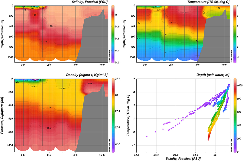
Figure 3. Hydrography during May 2014, transect D: Temperature, practical salinity, density.

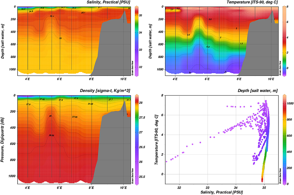
Figure 4. Hydrography during August 2014, transect D: Temperature, practical salinity, density.

The AW core at transect D was much less well confined in temperature and salinity in August than in January and May. In January 2014, transect B at roughly 20°E showed subduction of the AW core below slightly colder and fresher water (Figure 5). Colder and fresher waters (S = 34.4, T = −1°C, thus classified as SW) were present in the surface at bottom depths greater than 1000 m, indicating influence of polar water masses. May process stations repeated the pattern sampled on transect D during May (Figure 6). On-shelf (P1), surface waters were generally warmer and more saline (S > 34.6, T > 1°C), as opposed to stations further off-shelf (P4, S < 34.0, T < −0.5°C). Transect E and P6 and P7 showed warm AW of T > 5°C confined to the shelf slope at water depths < 200 m subducted under fresher, colder surface waters (Figure S3). Further off-shelf (water depths >200 m, north of 80.7°N), temperatures at intermediate depths (100–600 m) quickly dropped below 3°C, while still S > 34.92, indicating cooled AW.

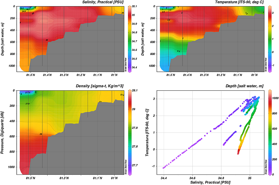
Figure 5. Hydrography during January 2014, transect B: Temperature, practical salinity, density.

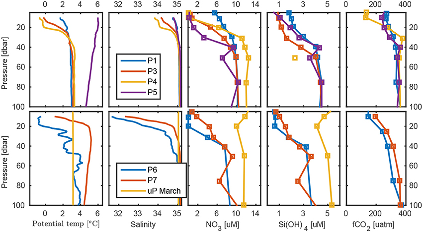
Figure 6. Temperature, salinity, ${\text{NO}}_3^{-}$, Si(OH)₄, and fCO₂ at process stations P1-P7 and the March station. The continental shelf is located toward the right (East), and Fram Strait to the left (West).

The six process stations and the March station are shown in Figure 6 (see also Figure S4). The evolution of hydrographic properties from P1 to P5 exemplifies the evolution of the shelf water mass distribution during summer. While the salinity profile was virtually unchanged, presumably due to an approximate balance between ice melt and advection of saline waters, the water column at P5 was warmed due to less cooling during the northward transport. A similar evolution was mirrored in the evolution from the March station to P6 and P7. March showed a deeply-mixed winter profile with AW extending completely up to the surface. The August profiles, in comparison, showed a warmer AW core below approximately 20 m and a transition layer to the cold, fresh meltwater above.

3.1.2. Inorganic Nutrients and Chlorophyll-a

The distribution of nutrients along the D transect in January (Figure 7) reflected the water mass distribution, with maximum concentrations at depths larger than 800 m for nitrate (${\text{NO}}_3^{-}$), phosphate (${\text{PO}}_4^{3-}$) and silicate (Si(OH)₄). Maximum concentrations of the different nutrients measured were 15.7 μM ${\text{NO}}_3^{-}$ and 11.9 μM Si(OH)₄ (both at 1,000 m, 8°E) and 1.07μM ${\text{PO}}_4^{3-}$ (1,000 m, 7°E). Also in May, maximum concentrations observed were 14.0 μM ${\text{NO}}_3^{-}$ (1,000 m, 6 °E), 1.10 μM ${\text{PO}}_4^{3-}$ and 9.76 μM Si(OH)₄ (both at 1,000 m, 5°E).

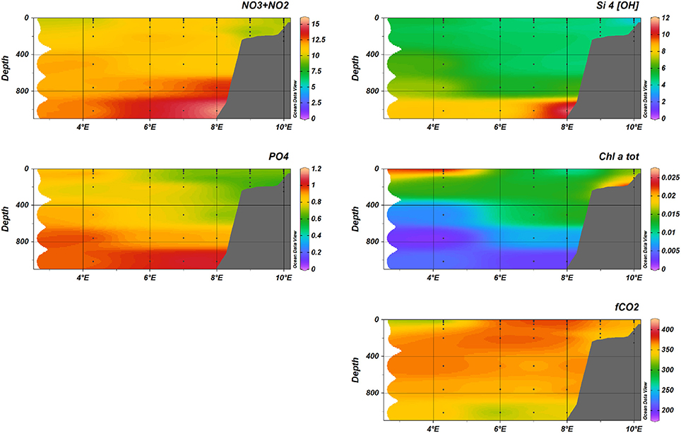
Figure 7. Nutrients (${\text{NO}}_3^{-}$+${\text{NO}}_2^{-}$, Si(OH)₄, ${\text{PO}}_4^{3-}$), fCO₂, and total Chlorophyll-a during January 2014, transect D.

At transect B in January (see Figure 8), the nutrient distribution in January indicated low concentrations in the SW off the shelf, compared to the water masses on and along the shelf. Also north of the Svalbard shelf, maximum concentrations of nutrients were found at >800 m depth.

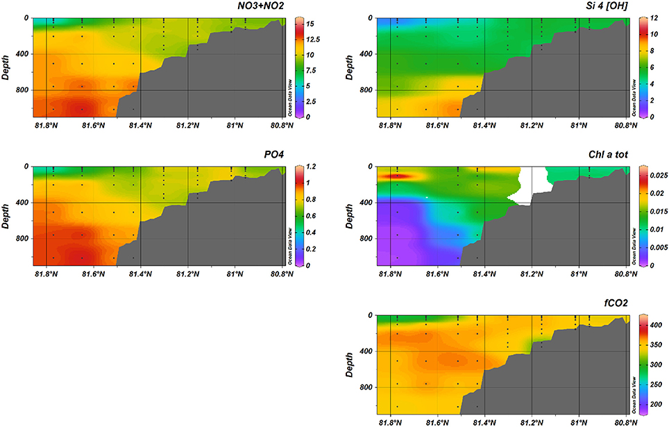
Figure 8. Nutrients (${\text{NO}}_3^{-}+$${\text{NO}}_2^{-}$, Si(OH)₄, ${\text{PO}}_4^{3-}$), fCO₂, and total Chlorophyll-a during January 2014, transect B.

The nutrient data also revealed two distinct regimes in the water masses present (Figure S1). Water above the AW (S maximum, NO₃≈10 μM, Si(OH)₄≈4.5 μM) followed a slope of approximately 1:2 in Si(OH)₄:${\text{NO}}_3^{-}$, while water below the AW-associated salinity maximum continued from there with a slope rather close to 2:1, indicating a different stochiometry in the remineralized nutrients accumulated in the deep.

3.2. Surface Layer Variability

3.2.1. Ice Cover and Mixed-Layer Evolution

Ice cover during the January, May and August cruises is plotted as ice concentrations in Figure 1. Table 1 lists ice concentrations for the process stations. All process stations (except for the ice-free P5) were conducted in ice conditions typical of the Marginal Ice Zone over the AW inflow, with ice concentrations varying between 25 and 90 %. They were therefore subject to rapid ice melt, and there was no clearly defined surface mixed layer, but rather a thin layer of fresher water, separated from the underlying water by a shallow (~10–15 m) pycnocline (see Table 1 and Figure S5). Since the photic zone extended deeper than these freshwater layers, photosynthesis may occur across the whole seasonal pycnocline, as we will see in Section 3.4. Essentially, this decoupled mixed layer nutrient budgets from productivity (Randelhoff et al., 2016).

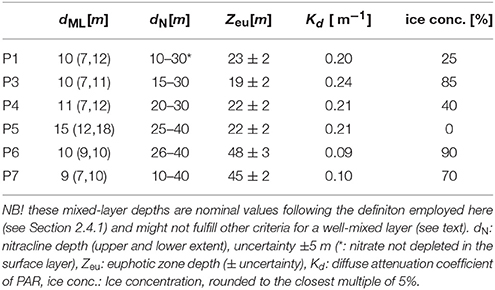
Table 1. Process station data. d_ML[m]: Median mixed-layer depth (in parentheses: observed range).

The temporal evolution of hydrographic properties at the D transect (Figure 9) demonstrates the contrast between the seasonality off and on the shelf slope. Off the shelf, seasonal stratification was stronger, had an earlier onset and was eroded later as distance from the shelf slope increases. A general pattern emerges where off-slope stations (e.g., the deeper parts of transect D and B) were stratified earlier and stronger than the stations on the upper shelf slope, which were unstratified even in January. Only in August a distinctly fresher surface layer was observed throughout the D transect. The relevant coordinate was the location with respect to both upper shelf slope (where the AW inflow lies) and the ice edge (where the meltwater input originates), seeing that a similar pattern was observed at P1-4.

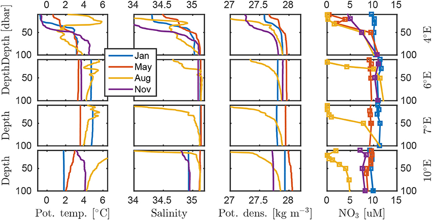
Figure 9. Temporal evolution of the hydrography on the D transect. The AW core is located closest to the 7°E station. The 4°E profile in November is from 2°E. Full-depth profiles of these data are found in Figure S11.

3.2.2. Nutrient Uptake Dynamics

As expected, Chl-a concentrations in January were negligible at < 0.025 mg Chl-a m⁻³. In May (see Figure 10), ${\text{NO}}_3^{-}$ was depleted at < 0.5 μM in the surface waters at the western part of transect D (4°E), increasing to ~2 μM at 7.5°E, reflecting a strong spring bloom with Chl-a concentrations >11 mg Chl-a m⁻³ in the surface waters. Chl-a concentrations >1 mg Chl-a m⁻³ were present to 50 m depth in this region. Further east (>8°E), higher nutrient concentrations and lower Chl-a concentrations indicated that the bloom along and above the shelf started later compared to the central Fram Strait this year.

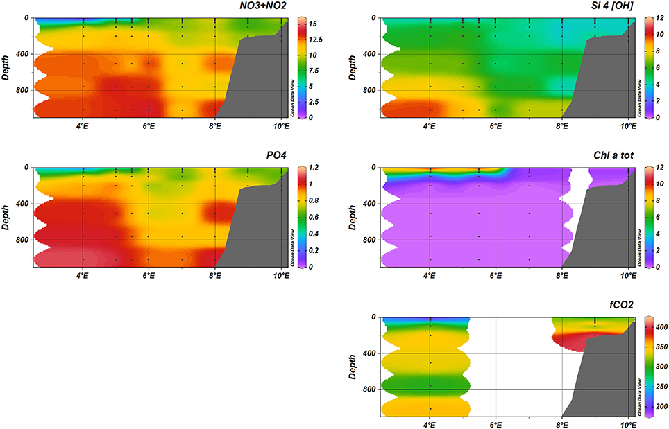
Figure 10. Nutrients (${\text{NO}}_3^{-}$+${\text{NO}}_2^{-}$, Si(OH)₄, ${\text{PO}}_4^{3-}$), fCO₂, and total Chlorophyll-a during May 2014, transect D.

In August (see Figure 11), elevated chl-a concentrations were observed in the surface waters across transect D, but with maximum values of 6 mg Chl-a m⁻³.

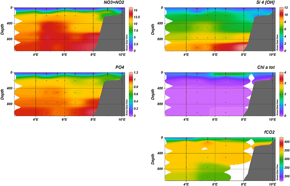
Figure 11. Nutrients (${\text{NO}}_3^{-}$+${\text{NO}}_2^{-}$, Si(OH)₄, ${\text{PO}}_4^{3-}$), fCO₂, and total Chlorophyll-a during August 2014, transect D.

${\text{NH}}_4^{+}$ levels in May were generally low, barely exceeding 0.5 μM under the pycnocline close to and in the MIZ (Figure 12, Figure S6). On-shelf on transect D, ${\text{NH}}_4^{+}$ levels were slightly elevated (>0.3 μM). August had a similar pattern, with elevated levels of ${\text{NH}}_4^{+}$ under the pycnocline (>0.5 μM) and increasing toward the shelf (P5, >1.5 μM and on-shelf on transect D, >2.5 μM; Figures S7, S8). In winter, ${\text{NH}}_4^{+}$ levels were low (mostly < 0.2 μM), apart from the (stratified) parts of transect B out into the basin, where values reached to a maximum of 0.75 μM at 10 m below the surface (data not shown).

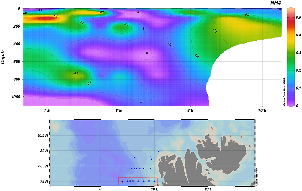
Figure 12. Ammonium ${\text{NH}}_4^{+}$ during May 2014, transect D.

The overall increase in ammonium values from May to August suggests that remineralization has started to take place and the community shifted toward a nutrient-recycling state. Notably, in the most stratified parts of transect B out into the basin, not all ${\text{NH}}_4^{+}$ has been removed. We hypothesize that this is related to the persisting stratification. To pinpoint the exact mechanism conclusively, further studies are needed; however, it seems plausible that the stratification inhibited downward mixing of the ${\text{NH}}_4^{+}$ left after the summer, possibly in concert with ongoing heterotrophic activity.

The timing of the mixed layer evolution coincides with the evolution of the water column nutrient inventory. All across the data set presented here we observe that the start of nutrient drawdown is closely tied to the development of a seasonal pycnocline. An interesting feature is that while nutrient drawdown starts earlier off-shelf (May drawdown of nitrate larger off-shelf than on-shelf), the trend in August drawdown is reversed (Figure 13; see also Figure S11). With some modifications (a general intensification of both horizontal and vertical gradients in hydrography) due to the ice edge overlaying the shelf slope, this picture is valid across the inflow region (data not shown due to lack of measurements of winter profiles) – assuming a winter concentration equal to the “deep” concentration homogeneous with depth, the same is valid for P1 to P4 (Figure 6; see also Figure S4) and another transect slightly north of transect D that has not been presented in this study due to its similarity to D).

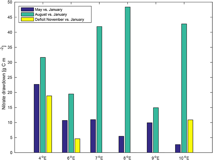
Figure 13. Temporal evolution of the upper ocean nitrate deficit (converted to carbon mass using the Redfield ratio) relative to the January values. The November deficit at 4°E was calculated using the 2°E November profile (cf. Figure 9). Note that advection is not taken into account here.

This is consistent with earlier reports of enhanced turbulent mixing over the shelf slope (Steele et al., 2012; Sarkar et al., 2015) which would ensure enhanced nutrient supply once the spring bloom is triggered, but we attempt no quantification beyond this qualitative observation.

Overall, Si was not entirely depleted in any of the samples, while ${\text{NO}}_3^{-}$ frequently was limiting. The straight mixing line in Si:${\text{NO}}_3^{-}$ space between the AW core and the surface suggests that the surface area represents an end member (i.e., a water mass) with NO₃ = 0 μM and Si(OH)₄≈0 μM. This would indicate a balance between overall drawdown of Si and N, that is an overall regional balance between the nutrient uptake of diatoms and of species that do not consume Si (like Phaeocystis), because Si:N ratios commonly observed in marine diatoms (Brzezinski, 1985) are around twice to three times as much as the observed Si:N slope of approximately 0.5 observed here.

3.3. CO₂ Fugacity

The fugacity of CO₂ (fCO₂) showed a clear spatial and temporal variability going from the shelf in the East to the deeper part of the Fram Strait further west. In January (see Figure 7), fCO₂ was relatively uniformly distributed with highest values of about 375 μatm in the upper 300 meters between 6 °E to 8 °E. On the shelf (9–10 °E) and west of 6 °E, values decreased likely due to colder water lowering fCO₂. At 4°E, we encountered the ice edge and the lowest values of 320 μatm may have been influenced by a combination of low temperatures and sea-ice melt water. Surrounding this water of higher fCO₂ in the core of the Atlantic water were relatively uniform values of about 350–375 μatm and lower values in the surface at about 4°E which coincided with the location of the ice edge. In May (see Figure 10), the lowest fCO₂ values were observed extending across the whole water column except for the highest values of 375 μatm that persisted in the AW core waters. The surface water (upper 30 meters) showed the most pronounced decrease and reached fCO₂ minima of about 225 μatm in the top 30 meters extending close to the shelf (8°E).

At the process stations, the surface waters showed fCO₂ undersaturation of about 150 μatm relative to the atmospheric values of about 400 μatm. We found large variability between 150 and 350 μatm in the upper 100 meters for all stations in May and August (Figure S9A). Below 200 meters, the fCO₂ showed similar values and little change between May and August. In the Intermediate Water (IW), below the core of the Atlantic Water, observed fCO2 values were about 350 μatm (Figure S9B). The off shelf values (P4) were about 125 μatm lower compared to the shelf fCO₂ (P1) values in the upper 30 meters (Figure S9B). The lower surface water fCO₂ off the shelf may have been due to stronger CO₂ uptake by phytoplankton than on shelf production, since the temperature was about 2°C higher at P1 (Figure 6), which only accounts for about 20 % of the fCO₂ increase on-shelf relative to the off-shelf value. Seasonal variability on the shelf (P1 and P5) showed decreased fCO₂ of about 25 μatm from May to August in the upper 30 meters. Below that depth the fCO₂ values were similar (Figure 6).

The low values in the surface water from May decreased and extended throughout the whole transect in August. Since temperature increased, this was likely due to biological CO₂ drawdown during phytoplankton production. This is supported by the strong decrease in nitrate and the increase in chlorophyll a between January and May in the same area and depth range. In August, increasing fCO₂ values were likely due to warming and a decline in the phytoplankton bloom. The increase may also partly have been due to net fCO₂ production from respiration of organic matter. In the Fram Strait, the strongest seasonal fCO₂ variability was not observed on the shelf (near Svalbard) but near the area of seasonal sea ice cover.

The range of fCO₂ levels in the surface water from this study can be compared with locations further east in the Arctic Ocean using data from ACSYS96 expedition (M. Chierici, unpublished data) and publicly available data from the Surface Ocean Carbon Dioxide Atlas (SOCAT, Bakker et al., 2016). In August in the northern Kara Sea at St. Anna Trough, fCO₂ ranges between 250 μatm to 390 μatm, which is similar to the fCO₂ levels we found both north and west of Svalbard. This is also similar to the values reported by SOCAT for the Laptev Sea. However, fCO₂ values are substantially lower in the surface waters in the East Siberia Sea and on the Chuckhi Sea shelf. Here, fCO₂ values were lower than 100 μatm in August 2005, which was explained to be due to substantial CO₂ uptake by phytoplankton (Fransson et al., 2009).

3.4. Depth of the Euphotic Zone

Euphotic zone depth (Z_eu) at spring 2014 stations were shallow, ranging between 19 and 23 m (Table 1, Figure S10). While a shallow Z_eu was also encountered in the summer at station P5 (Z_eu = 222 m, Table 1), euphotic zone depth at stations occupied north of Svalbard were overall deeper, ranging between 45 and 48 m. Calculated diffuse attenuation coefficients (K_d) showed a moderate positive relationship with mean water column chl-a concentration across all sampling stations (r² = 0.69; Figure S10);

The depth of the euphotic zone, where 1% of the incident radiation reaches the phytoplankton, was always deeper than the shallow meltwater lens that defines the mixed layer (Table 1). The vertical distribution of phytoplankton was also deeper than the mixed layer depth, with highest concentrations at the surface and starting to decrease at Z_eu. In this way, the irradiance profiles, and in particular Z_eu, reflected the seasonal phytoplankton development. Stations P1, P3, and P4 had shallow Z_eu with high surface chlorophyll concentrations; the euphotic zone deepened in the late summer coinciding with lower phytoplankton biomass, with the exception of P5 that maintained high chlorophyll at the surface. Lower chlorophyll concetrations translated to deeper Z_eu, twice as deep as in the spring, both in Arctic waters (P6) and Atlantic waters (P7) north of Svalbard. These latter two stations had similar optical properties and chlorophyll profiles than those reported by Granskog et al. (2015) for Atlantic Waters and the ice edge in the Fram Strait at 79°N, sampled a few weeks later in the same season. The Atlantic waters showed a broad subsurface chlorophyll maximum between 20 and 30 m depth, while the Ice Edge stations have a sharp and pronounced chlorophyll maximum at 25 m. This similarity indicates that the phytoplankton distribution in the Atlantic waters is maintained from West to North of Svalbard in late summer (i.e., from approximately 79°N, 0 to 9°E to 80° 41.12N, 14° 14.53E).

The diffuse attenuation coefficient (K_d), ranging from 0.09 to 0.24 m⁻¹ across the sampling stations, reflects the clarity of upper ocean waters. In our stations the magnitude of this parameter increases as the average euphotic zone chl-a concentration increases: K_d = 0.1229+0.0099·(chl-a), r² = 0.691 (Table 1, Figure S12A), with chl-a concentrations in turn significantly positively correlated with optical measured of turbidity (Figure S12B). While confirming the impact of phytoplankton on ocean optical properties, the positive intercept in Figure S12A also provides evidence for absorption by non-algal particles.

Previous sampling of the region by Pavlov et al. (2015) showed that absorption in the West Spitsbergen Current at 79°N in late summer (September) is dominated by particles, of which phytoplankton constituted a significant component. The K_d values of 0.15 and 0.17 m⁻¹ reported for the WSC, and euphotic depths of 37.4 and 41.9 m, indicate that waters upstream of the Carbon Bridge study area had somewhat higher phytoplankton concentration than the Atlantic inflow north of Svalbard (station P7).

3.5. Thermal Convection in Winter

The surface mixed layer over the shelf-slope was replete with nitrate on all stations in January 2014. Mooring data from earlier years at the shelf slope further downstream (30°E) confirm that this is part of a larger pattern, whereby the seasonal expansion of AW inflow along the shelf (Ivanov et al., 2009) slope breaks down the summer stratification as early as in December (Randelhoff et al., 2015), and preconditions deep-reaching (150–200 m) convection events, as was suggested by Aagaard et al. (1987) on the basis of a rather limited observational data set. The section B is located about 100 nautical miles upstream from those moorings, and therefore this specific feature of winter vertical thermohaline structure could be expected to be more pronounced here. However, in January 2014 the warming impact of AW on local hydrographic conditions was anomalously strong. In fact, AW reached the ocean surface over a distance of approximately 35 nautical miles across the shelf-slope (Figure 5). The warm water (with maximum temperature over 3°C) at the ocean surface contributed to keeping ice-free conditions (see Figure 1) and air temperature between zero and a few degrees below zero (data not shown). During the January survey, vertical thermal convection was still developing at the deep stations, while at the shallow stations (less than 200 m) convection had already reached the seabed. This is indicated by depth-uniform vertical distributions of temperature and salinity on shelf. Intensive vertical mixing aided replenishment of the nutrient pool in the photic zone, cf. Randelhoff et al. (2015).

Some reports claim evidence for wintertime, wind-driven upwelling in this area, and link this to primary productivity (e.g., Falk-Petersen et al., 2014). We have not found any indications to that effect during our sampling campaigns. For a more detailed description of the issue of wind-driven upwelling in Arctic shelfbreak areas, see Randelhoff and Sundfjord (2018). All else aside, even actual upwelling in winter would not enhance productivity in our study area since, as we have shown, the surface mixed layer is already replete by that time and well before the onset of the next spring bloom.

Vertical homogeneity in oxygen saturation also suggests a possible oxygenation of intermediate waters. However, attempts at answering this issue using our data set remain inconclusive since the difference between values of oxygen saturation at the surface and at 400 m depth inferred from a CTD-mounted SBE43 dissolved oxygen sensor (transect E, summer: approximately 75%, transect B, winter: approximately 79%) was small, and because we lack sufficiently precise Winkler oxygen measurements. In a more general context, the large heat content of inflowing AW in combination with depleted ice cover in the fall of 2013 provided a long-living anomaly of ice concentration north and north-east of Svalbard in winter 2014 (Ivanov et al., 2016). This anomaly in ice cover might have impacted both processes in the ocean and in the atmosphere.

4. Synthesis and Conclusions

The Atlantic inflow area west and north of Svalbard is a dynamic one, where warm, saline AW meets Arctic Water and sea ice, leading to an influx of fresh and cold meltwater. Both sea ice and Atlantic Water are continually being advected into the area. This tug of war leads to a fine balance in the development of the shallow, strongly stratified seasonal pycnocline in summer and its erosion in winter. Seasonal, light-dominated biological processes therefore take place at the fringes of the large-scale hydrography and are not easily represented by large-scale, long-time averages. Understanding seasonal and local aspects of stratification and mixing processes is thus necessary in order to correctly couple biology and biogeochemistry to their physical drivers.

Based on the data presented in this study, we make the following conclusions: (1) Atlantic Water (AW) and cold Atlantic Water (cAW) are the dominant water masses in the area. While this finding is hardly new, it is worth keeping in mind that most samples acquired during the CarbonBridge campaign are taken from waters of Atlantic origin that are cooled and freshened on a seasonal basis as opposed to originating from the central Arctic Ocean. (2) Northward penetration of temperature-stratified AW permits thermal convection in winter and thus high heat fluxes, potentially keeping the area ice-free in winter. The AW influence documented here and elsewhere thus permits rapid replenishment of nutrients around the shelf slope. (3) The timing of nutrient and fCO₂ drawdown is closely linked to the development of a seasonal pycnocline (see also Marit Reigstad et al., “Bloom stage characteristics in an Atlantic-influenced Arctic marine ecosystem and implications for future productivity pathways,” this issue). However, for nitrate, the seasonally integrated drawdown can depend on other parameters and tends to be larger on than off the shelf.

Ice extent in our study area is notoriously dominated by the wind field from seasonal to interannual scales (e.g., Koenigk et al., 2009), and we do therefore not assume that the exact distribution (i.e., based on latitude-longitude-referenced maps) of the parameters that we found in our data set is exactly reproduced during other years. However, patterns should be similar interannually when referenced to the relative positions of the AW core, the ice edge and the seasonal freshwater layer, which in our data set are tightly coupled to the biogeochemistry.

We summarized our central conclusions about the seasonal and geographic distribution of hydrography, mixing, and consequently biogeochemistry in a schematic: see Figure 14.

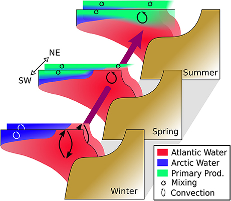
Figure 14. Schematic summarizing the major seasonal and spatial hydrographic patterns described in this study. Shown are the water masses, mixing processes, and primary priduction in six conceptual cross-shelf transects. For each season (in our data represented by the months January, May, August), there are two transects, one further south and west (in our data: transect D) and one further north and east (our transects B, E, and various process stations; see Figure 1). Further northeast, more ice is present, stratifying the Atlantic inflow earlier, with a concomitant earlier bloom. Once the Atlantic inflow is stratified and the spring bloom has started also further southwest (see the “Summer” transect), the nutrient consumption even reaches deeper, presumably due to weaker stratification, hence deeper mixing.

All of these findings indicate that under a scenario of increased “Atlantification” of the shelf slope north of Svalbard, this area will indeed likely become a regional hotspot with increased primary production due to efficient transport and vertical supply of nutrients coupled with decreased light limitation due to oceanic heat.

Author Contributions

AR: led the overall data analysis and writing of the paper; MR: led the analysis of the nutrient and chlorophyll-a data; MCh: led the analysis of the fCO₂ data; MCa: led the analysis of the radiation profiles; MR, MCh, AS, VI, MCa, MV, J-ÉT, and GB: contributed to the writing; MR, MCh, AS, and MCa: helped produce the figures. All authors contributed to data analysis.

Conflict of Interest Statement

The authors declare that the research was conducted in the absence of any commercial or financial relationships that could be construed as a potential conflict of interest.

Acknowledgments

This study was funded by the Norwegian Research Council projects CARBON BRIDGE, a Polar Programme (project 226415) funded by the Norwegian Research Council, and MicroPolar (NRC no. 225956/E10).

MCa was supported by NASA Headquarters under the NASA Earth and Space Science Fellowship Program grant NNX12AN48H. We also thank funding from the US National Science Foundation award PLR-071443733 to MV. Jorun Karin Egge contributed with chlorophyll data for March and November. We are also grateful to Elena Perez and University of Tromsø technician Hans Dybvik for help in the field. We thank captain and crew of R/Vs Helmer Hanssen and Lance and all scientists aboard for their help during the field campaigns. VI's contribution was supported by the RFBR grant#17-05-00558.

All data are made available to the public, see PANGEA (https://www.pangaea.de), the Norwegian Polar Data Centre (https://data.npolar.no) (for hydrographic data), the Norwegian Marine Data Centre (https://www.nmdc.no) and GLODAP (Global Ocean Data Analysis Project for Carbon, https://climatedataguide.ucar.edu/climate-data/glodap-global-ocean-data-analysis-project-carbon), the latter two for carbonate system data.

Supplementary Material

The Supplementary Material for this article can be found online at: https://www.frontiersin.org/articles/10.3389/fmars.2018.00224/full#supplementary-material

References

Aagaard, K., Foldvik, A., and Hillman, S. R. (1987). The west spitsbergen current: disposition and water mass transformation. J. Geophys. Res. 92:3778. doi: 10.1029/JC092iC04p03778
Årthun, M., Eldevik, T., Smedsrud, L. H., Skagseth, O., and Ingvaldsen, R. B. (2012). Quantifying the Influence of Atlantic Heat on Barents Sea Ice Variability and Retreat. J. Climate 25, 4736–4743. doi: 10.1175/JCLI-D-11-00466.1
Bakker, D. C. E., Pfeil, B., Landa, C. S., Metzl, N., O'Brien, K. M., Olsen, A., et al. (2016). A multi-decade record of high-quality fco2 data in version 3 of the surface ocean co2 atlas (socat). Earth Syst. Sci. Data 8, 383–413. doi: 10.5194/essd-8-383-2016
Berge, J., Renaud, P. E., Darnis, G., Cottier, F., Last, K., Gabrielsen, T. M., et al. (2015). In the dark: a review of ecosystem processes during the arctic polar night. Progr. Oceanogr. 139, 258–271. doi: 10.1016/j.pocean.2015.08.005
Beszczynska-Möller, A., Fahrbach, E., Schauer, U., and Hansen, E. (2012). Variability in Atlantic water temperature and transport at the entrance to the Arctic Ocean, 1997-2010. ICES J. Mar. Sci. 69, 852–863. doi: 10.1093/icesjms/fss056
Brzezinski, M. A. (1985). The Si:C:N ratio of marine diatoms: interspecific variability and the effect of some environmental variables. J. Phycol. 21, 347–357. doi: 10.1111/j.0022-3646.1985.00347.x
Codispoti, L., Flagg, C., Kelly, V., and Swift, J. H. (2005). Hydrographic conditions during the 2002 SBI process experiments. Deep Sea Res. II Top. Stud. Oceanogr. 52, 3199–3226. doi: 10.1016/j.dsr2.2005.10.007
de Steur, L., Hansen, E., Mauritzen, C., Beszczynska-Möller, A., and Fahrbach, E. (2014). Impact of recirculation on the east greenland current in fram strait: Results from moored current meter measurements between 1997 and 2009. Deep Sea Res. I Oceanogr. Res. Pap. 92, 26–40. doi: 10.1016/j.dsr.2014.05.018
Dickson, A., and Millero, F. (1987). A comparison of the equilibrium constants for the dissociation of carbonic acid in seawater media. Deep Sea Res. A Oceanogr. Res. Pap. 34, 1733–1743. doi: 10.1016/0198-0149(87)90021-5
Dickson, A. G. (1990). Standard potential of the reaction: AgCl(s) + 12H2(g) = Ag(s) + HCl(aq), and the standard acidity constant of the ion in synthetic sea water from 273.15 to 318.15 K. J. Chem. Thermodyn. 22, 113–127. doi: 10.1016/0021-9614(90)90074-Z
Falk-Petersen, S., Pavlov, V., Berge, J., Cottier, F., Kovacs, K. M., and Lydersen, C. (2014). At the rainbow's end: high productivity fueled by winter upwelling along an Arctic shelf. Polar Biol. 38, 5–11. doi: 10.1007/s00300-014-1482-1
Fransson, A., Chierici, M., and Nojiri, Y. (2009). New insights into the spatial variability of the surface water carbon dioxide in varying sea ice conditions in the Arctic Ocean. Contin. Shelf Res. 29, 1317–1328. doi: 10.1016/j.csr.2009.03.008
Granskog, M. A., Pavlov, A. K., Sagan, S., Kowalczuk, P., Raczkowska, A., and Stedmon, C. A. (2015). Effect of sea-ice melt on inherent optical properties and vertical distribution of solar radiant heating in arctic surface waters. J. Geophys. Res. Oceans 120, 7028–7039. doi: 10.1002/2015JC011087
Holm-Hansen, O., and Riemann, B. (1978). Chlorophyll a determination: improvements in methodology. Oikos 30, 438–447. doi: 10.2307/3543338
Holmes, R. M., Aminot, A., Kérouel, R., Hooker, B. A., and Peterson, B. J. (1999). A simple and precise method for measuring ammonium in marine and freshwater ecosystems. Can. J. Fish. Aqua. Sci. 56, 1801–1808. doi: 10.1139/f99-128
Ivanov, V., Alexeev, V., Koldunov, N. V., Repina, I., Sandø, A. B., Smedsrud, L. H., et al. (2016). Arctic Ocean heat impact on regional ice decay-a suggested positive feedback. J. Phys. Oceanogr. 46, 1437–1456. doi: 10.1175/JPO-D-15-0144.1
Ivanov, V. V., Polyakov, I. V., Dmitrenko, I. A., Hansen, E., Repina, I. A., Kirillov, S. A., et al. (2009). Seasonal variability in Atlantic Water off Spitsbergen. Deep Sea Res. I Oceanogr. Res. Pap. 56, 1–14. doi: 10.1016/j.dsr.2008.07.013
Jones, E. P., Anderson, L. G., and Swift, J. H. (1998). Distribution of Atlantic and Pacific waters in the upper Arctic Ocean: implications for circulations. Geophys. Res. Lett. 25, 765–768. doi: 10.1029/98GL00464
Kirk, J. T. O. (2010). Characterizing the underwater light field. Light Photosynth. Aquat. Ecosyst. 114, 133–152. doi: 10.1017/CBO9781139168212.007
Koenig, Z., Provost, C., Villacieros-Robineau, N., Sennéchael, N., Meyer, A., Lellouche, J.-M., et al. (2017). Atlantic waters inflow north of Svalbard: insights from IAOOS observations and Mercator Ocean global operational system during N-ICE2015. J. Geophys. Res. Oceans 122, 1254–1273. doi: 10.1002/2016JC012424
Koenigk, T., Mikolajewicz, U., Jungclaus, J. H., and Kroll, A. (2009). Sea ice in the Barents Sea: seasonal to interannual variability and climate feedbacks in a global coupled model. Climate Dyn. 32, 1119–1138. doi: 10.1007/s00382-008-0450-2
Marnela, M., Rudels, B., Houssais, M.-N., Beszczynska-Möller, A., and Eriksson, P. B. (2013). Recirculation in the Fram Strait and transports of water in and north of the Fram Strait derived from CTD data. Ocean Sci. 9, 499–519. doi: 10.5194/os-9-499-2013
Mehrbach, C., Culberson, C. H., Hawley, J. E., and Pytkowicx, R. M. (1973). Measurement of the apparent dissociation constants of carbonic acid in seawater at atmospheric pressure. Limnol. Oceanogr. 18, 897–907. doi: 10.4319/lo.1973.18.6.0897
Meyer, A., Sundfjord, A., Fer, I., Provost, C., Villacieros Robineau, N., Koenig, Z., et al. (2017). Winter to summer oceanographic observations in the Arctic Ocean north of svalbard. J. Geophys. Res. Oceans 122, 6218–6237. doi: 10.1002/2016JC012391
Onarheim, I. H., Smedsrud, L. H., Ingvaldsen, R. B., and Nilsen, F. (2014). Loss of sea ice during winter north of svalbard. Tellus A 114–66. doi: 10.3402/tellusa.v66.23933
Pavlov, A. K., Granskog, M. A., Stedmon, C. A., Ivanov, B. V., Hudson, S. R., and Falk-Petersen, S. (2015). Contrasting optical properties of surface waters across the fram strait and its potential biological implications. J. Mar. Syst. 143, 62–72. doi: 10.1016/j.jmarsys.2014.11.001
Pfirman, S. L., Colony, R., NÃrnberg, D., Eicken, H., and Rigor, I. (1997). Reconstructing the origin and trajectory of drifting Arctic sea ice. J. Geophys. Res. Oceans 102, 12575–12586. doi: 10.1029/96JC03980
Pierrot, D., Lewis, E., and Wallace, D. (2006). MS Excel program developed for CO2 system calculations. ORNL/CDIAC-105a. Carbon Dioxide Information Analysis Center; Oak Ridge National Laboratory; US Department of Energy; Oak Ridge, TN.
Polyakov, I. V., Pnyushkov, A. V., Alkire, M. B., Ashik, I. M., Baumann, T. M., Carmack, E. C., et al. (2017). Greater role for Atlantic inflows on sea-ice loss in the Eurasian Basin of the Arctic Ocean. Science 356, 285–291. doi: 10.1126/science.aai8204
Polyakov, I. V., Pnyushkov, A. V., and Timokhov, L. A. (2012). Warming of the intermediate Atlantic water of the Arctic Ocean in the 2000s. J. Climate 25, 8362–8370. doi: 10.1175/JCLI-D-12-00266.1
Randelhoff, A., Fer, I., and Sundfjord, A. (2017). Turbulent upper-ocean mixing affected by meltwater layers during Arctic summer. J. Phys. Oceanogr. 47, 835–853. doi: 10.1175/JPO-D-16-0200.1
Randelhoff, A., Fer, I., Sundfjord, A., Tremblay, J.-E., and Reigstad, M. (2016). Vertical fluxes of nitrate in the seasonal nitracline of the Atlantic sector of the Arctic Ocean. J. Geophys. Res. Oceans 121, 5282–5295. doi: 10.1002/2016JC011779
Randelhoff, A., and Sundfjord, A. (2018). Short commentary on marine productivity at arctic shelf breaks: upwelling, advection and vertical mixing. Ocean Sci. 14, 293–300. doi: 10.5194/os-14-293-2018
Randelhoff, A., Sundfjord, A., and Reigstad, M. (2015). Seasonal variability and fluxes of nitrate in the surface waters over the Arctic shelf slope. Geophys. Res. Lett. 42, 3442–3449. doi: 10.1002/2015GL063655
Rudels, B., Korhonen, M., Schauer, U., Pisarev, S., Rabe, B., and Wisotzki, A. (2015). Circulation and transformation of Atlantic water in the Eurasian Basin and the contribution of the Fram Strait inflow branch to the Arctic Ocean heat budget. Progr. Oceanogr. 132, 128–152. doi: 10.1016/j.pocean.2014.04.003
Sarkar, S., Sheen, K. L., Klaeschen, D., Brearley, J. A., Minshull, T. A., Berndt, C., et al. (2015). Seismic reflection imaging of mixing processes in Fram Strait. J. Geophys. Res. Oceans 120, 6884–6896. doi: 10.1002/2015JC011009
Slagstad, D., Wassmann, P. F. J., and Ellingsen, I. (2015). Physical constrains and productivity in the future arctic ocean. Front. Mar. Sci. 2:85. doi: 10.3389/fmars.2015.00085
Spreen, G., Kaleschke, L., and Heygster, G. (2008). Sea ice remote sensing using AMsr-e 89-GHz channels. J. Geophys. Res. 113:C02S03. doi: 10.1029/2005JC003384
Steele, E., Boyd, T., Inall, M., Dumont, E., and Griffiths, C. (2012). Cooling of the West Spitsbergen Current: AUV-based turbulence measurements west of Svalbard. 2012 IEEE/OES Autonomous Underwater Vehicles (AUV) (Southampton).
Torres-Valdés, S., Tsubouchi, T., Bacon, S., Naveira-Garabato, A. C., Sanders, R., McLaughlin, F. A., et al. (2013). Export of nutrients from the Arctic Ocean. J. Geophys. Res. Oceans 118, 1625–1644. doi: 10.1002/jgrc.20063
Untersteiner, N. (1988). On the ice and heat balance in Fram Strait. J. Geophys. Res. Oceans 93, 527–531. doi: 10.1029/JC093iC01p00527
Keywords: Arctic Ocean, Atlantic water, hydrography, shelf slope, nutrients, carbon, fram strait, barents sea
Citation: Randelhoff A, Reigstad M, Chierici M, Sundfjord A, Ivanov V, Cape M, Vernet M, Tremblay J-É, Bratbak G and Kristiansen S (2018) Seasonality of the Physical and Biogeochemical Hydrography in the Inflow to the Arctic Ocean Through Fram Strait. Front. Mar. Sci. 5:224. doi: 10.3389/fmars.2018.00224
Received: 23 March 2018; Accepted: 11 June 2018;
Published: 29 June 2018.
Edited by:
Dorte Krause-Jensen, Aarhus University, DenmarkReviewed by:
Kalle Olli, University of Tartu, EstoniaWilliam Gerald Ambrose Jr., Bates College, United States
Copyright © 2018 Randelhoff, Reigstad, Chierici, Sundfjord, Ivanov, Cape, Vernet, Tremblay, Bratbak and Kristiansen. This is an open-access article distributed under the terms of the Creative Commons Attribution License (CC BY). The use, distribution or reproduction in other forums is permitted, provided the original author(s) and the copyright owner(s) are credited and that the original publication in this journal is cited, in accordance with accepted academic practice. No use, distribution or reproduction is permitted which does not comply with these terms.
*Correspondence: Achim Randelhoff, achim.randelhoff@takuvik.ulaval.ca