

Abstract
Only meters below our feet, shallow aquifers serve as sustainable energy source and provide freshwater storage and ecological habitats. All of these aspects are crucially impacted by the thermal regime of the subsurface. Due to the limited accessibility of aquifers however, temperature measurements are scarce. Most commonly, shallow groundwater temperatures are approximated by adding an offset to annual mean surface air temperatures. Yet, the value of this offset is not well defined, often arbitrarily set, and rarely validated. Here, we propose the usage of satellite-derived land surface temperatures instead of surface air temperatures. 2 548 measurement points in 29 countries are compiled, revealing characteristic trends in the offset between shallow groundwater temperatures and land surface temperatures. Here it is shown that evapotranspiration and snow cover impact on this offset globally, through latent heat flow and insulation. Considering these two processes only, global shallow groundwater temperatures are estimated in a resolution of approximately 1 km × 1 km. When comparing these estimated groundwater temperatures with measured ones a coefficient of determination of 0.95 and a root mean square error of 1.4 K is found.
Export citation and abstract BibTeX RIS

Original content from this work may be used under the terms of the Creative Commons Attribution 3.0 licence.
Any further distribution of this work must maintain attribution to the author(s) and the title of the work, journal citation and DOI.
1. Introduction
Sustainable water resources and energy supply are two of the main challenges in today's society (e.g. Gleeson et al 2012, Gleeson et al 2016, Jaramillo and Destouni 2015), (Potocnik 2007, Kammen and Sunter 2016). Shallow groundwater temperatures play a crucial role in both of these challenges. For example, they affect microbial activity in aquifers thus, giving a unique insight into oxygen depletion in huge quantities of the Earth's water supply (Danielopol et al 2003), and are the key factor to determining the usability and the potential of shallow geothermal energy (Stauffer et al 2013, Zhu et al 2010, Rivera et al 2017). Additionally, the temperatures of the surface and subsurface are closely linked. The coupling between both is utilized to reconstruct ground surface temperature histories using both borehole temperature data (Taniguchi et al 2005, Beltrami et al 2015) and noble gas temperatures (Cey 2009), and to analyze the impact of climate change on the subsurface (Taylor et al 2012, Menberg et al 2014, Pollack et al 1998). There is growing interest in understanding the effect of the thermal and hydrogeological regime of the subsurface on climate (Maxwell and Kollet 2008). A main hurdle, however, is the uncertainty of shallow groundwater temperature (GWT) distribution. Since direct measurements are scarce and measurement points are limited, GWT is typically estimated by adding an offset to annual mean surface air temperatures. While the existence of this offset has long been discussed (Kappelmeyer and Haenel 1974), its value has yet to be validated on a larger scale.
In a closed system without latent heat, the surface energy balance predicts near surface temperatures and shallow subsurface temperatures to be in equilibrium. Studies in warm or moderate climates have shown the offset between these to be close to zero (Čermák et al 2014), however on the global scale it is highly variable. Latent heat flow caused by evapotranspiration (ET) plays a key role in the surface energy balance. Its effects on surface climate have been thoroughly discussed (Shukla and Mintz 1982) and it has been determined that an increase in ET will decrease measured surface temperatures (Sun et al 2016). Additionally, ET is closely linked to natural precipitation and recharge (Scanlon et al 2002). This effect is most often discussed in regards to groundwater availability in changing climates (Döll 2009, Shah 2009); however recharge also affects shallow GWTs directly (Anderson 2005). Still, the effect of ET on the offset between land surface temperature (LST) and GWT is unknown.
In higher and colder latitudes the offset is often dominated by snow. Here, with its low thermal conductivity, the snow cover functions as an insulator and prevents the conduction of cold surface temperatures into the subsurface layer (Zhang 2005). Studies set in northern regions found subsurface temperatures to be significantly warmer than surface temperatures (Banks et al 2004, Hachem et al 2012).
On a regional scale, shallow GWT is also influenced by a multitude of factors such as anthropogenic heat flux (Benz et al 2015), geothermal hot spots, groundwater flow, and groundwater depth (Fan et al 2013) since temperature typically increases with depth.
In this study the offset between surface and subsurface temperatures is analyzed on a global scale. Since annual mean surface air temperatures are only available in areas, where long-term monitoring stations are installed, we propose the use of satellite-derived land surface temperatures (LST) instead. By comparing a global dataset of measured GWT with decadal mean LST, we determine and analyze the offset ΔT = GWT − LST and quantify the influence from evapotranspiration (ET) and snow cover. Other more regional influences cannot be addressed globally. Finally, the offset and therefore GWTs are estimated on a global scale using only satellite-derived data.
2. Material and methods
2.1. Groundwater temperatures
Overall, 2548 shallow measurement points in 29 countries and two overseas territories were compiled that provide (multi)-annual mean groundwater temperatures (GWT) without a seasonal bias (figure 1, table S1 stacks.iop.org/ERL/12/034005/mmedia). The distribution of GWT data is uneven and has a bias towards the northern hemisphere, with only 14% of all measurement points being located south of the equator. However, this is not considered crucial since the offset between GWT and land surface temperature (LST) in both hemispheres show similar behavior for equal latitudes (figure S1). Because all measurement points are south of 61° latitude, GWTs closer to the polar region are not addressed. Following the commonly used land cover classification system (LCCS) and GlobCover (2009) data, we find that 53% of all measurement points are located in cultivated terrestrial areas and managed lands, 37% in natural and semi-natural terrestrial vegetation, and 9% in artificial surfaces. A study in Germany found GWTs under artificial surfaces and cultivated lands to be elevated compared to their rural surrounding by approximately 2.0 ± 0.7 K and 0.2 ± 0.8 K, respectively (Benz et al 2017).

Figure 1 Global map of land surface temperature (LST) and shallow groundwater temperature (GWT). LST is given as the 10 year mean (01/2005–12/2014) of daily MODIS products MOD11A1 and MYD11A1. The bias towards cloud free days was corrected in respect to seasonal cloud cover variations. (Multi)-annual mean GWTs were collected during the same time period in a depth of down to 60 m below ground.
Download figure:
Standard image High-resolution imageAll measurements were performed in a depth of less than 60 m, including springs, since this is the minimum depth that a temperature signal penetrates in 10 years (Taylor and Stefan 2009, Whittington et al 2009). However, the majority of the points correspond to measurements in a depth of no less than 30 m. At each measurement point, GWTs were read at least once in the time frame of 01/Jan/2005 to 31/Dec/2014. While temperatures measured in a depth of more than 20 m generally do not indicate any seasonal influences (Beltrami and Kellman 2003), temperatures measured above this depth do (Taylor and Stefan 2009). Hence, the temperatures have to be measured uniformly over the span of the various seasons to generate a bias-free mean. To estimate whether the mean temperature of a measurement location is biased by seasonal temperature variations, a variable called seasonal radius r is introduced. It determines whether measurements were taken uniformly over the span of the seasons (r = 0) or if all measurements were taken in the same month (r = 1). To determine r, every measurement of a time series is first converted to a vector with a length of 1.0 and a direction corresponding to the month of measurements. Next, the mean of all measurement-vectors of a single measurement point is determined. The length of the resulting mean vector is the seasonal radius. Figure S2(a) gives an example of a well that was measured twice, once in November and once in June. Figure S2(b) depicts the seasonal radii of all analyzed measurement points with a measurement depth of less than 20 m located in France and its overseas territories (table S1). The influence of this seasonal radius on GWTs was analyzed and it was found that measurement points with a seasonal radius ≤ 0.25 can be considered bias free (figure S3). Hence, the following rules for measurement point selection were determined:
- The maximum measurement depth is 60 m.
- If the measurement depth is ≤20 m, only points that have a seasonal radius of ≤0.25 were considered.
- If the measurement depth is not known, only points that have a well depth ≤60 m and a seasonal radius ≤0.25 were considered.
- If neither measurement depth nor well depth are known but the raw data show seasonal variations of more than 1 K, points with a seasonal radius ≤0.25 were considered.
- If temperatures were taken after pumping, only points with a well depth between 20 m and 60 m were considered.
2.2. Land surface temperatures
To determine the 10 year arithmetic mean (01/2005–12/2014) of land surface temperatures (LST) we used MODIS daily products MOD11A1 and MYD11A1 (Wan and Dozier 1996, Wan 1999), as obtained from NASA's TERRA and AQUA satellites, courtesy of the NASA Land Processes Distributed Active Archive Center (LP DAAC), USGS/Earth Resources Observation and Science (EROS) Center, Sioux Falls, South Dakota, https://lpdaac.usgs.gov. Each satellite views the entire planet twice daily giving four LST measurements a day. MODIS-derived LSTs have been previously validated by several studies (Ermida et al 2014, Guillevic et al 2014, Wan et al 2002, Trigo et al 2008). Because LSTs are only retrieved for clear sky observations, they have a bias towards non cloudy days. Due to the seasonal cycle of cloud cover (Wylie and Menzel 1999), this 'clear sky'-bias displays in part as a seasonal bias. To consider this bias, the 10 year mean was determined in three steps. First, the mean temperature of each month was determined for the years 2005 to 2014. Out of these, the 10 year mean for each month was determined before combining them to a single 10 year mean map. This was performed using Google Earth Engine and was exported in a resolution of approximately 1 km × 1 km (0.009° × 0.009°) (figure 1).
Over the analyzed 10 year time period no significant change in global LST is observed (figure S4). Hence, climate change was not consider when comparing 10 year mean LSTs with GWTs that were often measured only towards the end of the late analyzed 10 year time period.
2.3. Evapotranspiration
Evapotranspiration data were gathered from the Noah 2.7.1 model in the Global Land Data Assimilation System (GLDAS) data products Version 1 (Rodell et al 2004) (spatial resolution: 0.24°). These evapotranspiration data have previously been validated by several studies (Rodell et al 2011, Mueller et al 2011, Wang et al 2011, Kato et al 2007). In this study, the decadal mean (01/2005–12/2014) evapotranspiration (ET) was determined using the Google Earth Engine and was exported in a resolution of approximately 1 km × 1 km.
2.4. Snow days
Information on snow days was derived from MODIS Terra and Aqua Snow Cover Daily L3 Global 500 m Grid, Version 5 (Hall et al 2006), products MOD10A1 and MYD10A1, courtesy of the National Snow and Ice Data Center (NSIDC). The data have previously been validated by several studies (Gladkova et al 2012, Klein and Stroeve 2002, Tekeli et al 2006). Using Google Earth Engine, the percentage of snow days in the 10 years from 01/2005 to 12/2014 was determined by dividing the number of days classified as 'snow' by the sum of the days classified as either 'no snow' or 'snow'. The data were exported in a resolution of approximately 1 km × 1 km.
2.5. Estimating groundwater temperatures
In this study GWTs are estimated using satellite-derived data only. Two distinct effects on the offset between GWT and LST are quantified: snow cover insulates warm groundwater temperatures and latent heat flux, caused by evapotranspiration, factors into the surface energy balance, thus decreasing LSTs. The total offset,  can be described as the superposition of the offsets caused by evapotranspiration (
 ) and the offsets caused by the duration of snow cover (
 ). The latter is quantified as the percentage of snow days during the analyzed 10 years. Because both pairs (ET and latent heat, and snow days and insulation) are linearly dependent, a linear fit
  is used to estimate the global offset. Fitting was performed in MATLAB R2013a with the function 'nlinfit' for nonlinear regression. The coefficients are estimated using iterative least squares estimation. Initial values are
  and
and  . The 95% prediction interval half-width for a new observation was determined using the function 'nlpredci'.
3. Results and discussion
The compiled ten year mean land surface temperatures (LST) and (multi)-annual mean groundwater temperatures (GWT) are displayed in figure 1. For 83% of all measurement points, GWTs are warmer than LST. The average offset  is 1.2 ± 1.5 K (figure S6). The influence of GWT measurement depth on the offset was analyzed for all measurement points with a known measurement depth (Austria, France and its overseas territories, table S1). It revealed an increase in temperature by only 0.02 K m−1 (figure S5), agreeing well with other reported values such as the average UK geothermal gradient of 0.026 K m−1 (Busby et al 2009) and a simulate gradients of 024 K m−1 for a realistic geothermal heat flux of 0.05 W m−2 (Wagner et al 2012). Consequently, the impact of depth on mean groundwater temperature (GWT) was disregarded.
Overall the lowest offset is −6.1 K (LST: 16.5 °C; GWT: 10.5 °C, daily measurements from 01/2013 to 05/2014) in a spring in the Black Rock Desert—High Rock Canyon Emigrant Trails National Conservation Area, Nevada, USA (figure S7(b), table S1). The highest offset of 11.0 K (LST: 2.0 °C; GWT: 13 °C, one measurement in 06/2005 at a depth in between 21 and 40 m below ground) is measured in Erdenet, Mongolia (figure S7(c), table S1). It is plausible that the high GWT is caused by the subsurface urban heat island phenomenon (Menberg et al 2013), where GWTs are raised by anthropogenically induced heat flow (Benz et al 2015) from underground structures such as buildings or, in this specific case, the local copper-molybdenum mine (Battogtokh et al 2013).
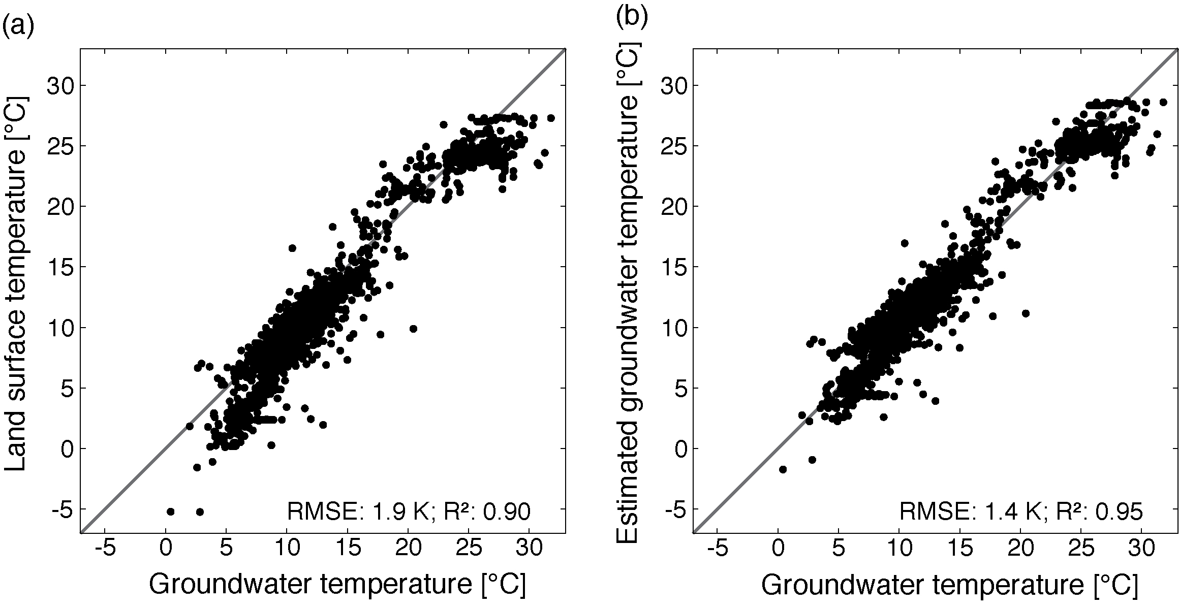
Despite these extreme examples, global GWT and LST values correlate well, with a Pearson correlation coefficient of 0.97, a coefficient of determination (R2) of 0.90 and a root mean square error (RMSE) of 1.9 K (figure 2(a)). As expected, the data indicate that GWTs are elevated compared to LSTs for the coldest and warmest temperatures. These differences are caused by the two distinct effects discussed previously: in areas with lower temperatures snow cover insulates warm groundwater temperatures during the winter month raising the annual mean; in warmer and more humid areas latent heat flux caused by evapotranspiration (ET) factors into the surface energy balance, thus decreasing LSTs. Several measurement points located in moderate climate regions are affected by both factors (figure S8). Hence, the offset between GWT and LST is discussed as a superposition of an offset caused by ET and an offset caused by snow cover ( ).
).

Figure 2 Relationship between (a) groundwater temperature (GWT) and land surface temperature (LST) and (b) estimated and measured GWT. The line of equality is given in dark grey.
Download figure:
Standard image High-resolution image3.1. Estimating groundwater temperatures
The influence of evapotranspiration (ET) on the offset is displayed in figure 3(a). As expected, an increase in ET raises  . However, measurement points in arid regions such as Chile, the western USA, and the Arabian Peninsula with a low ET have a negative offset, indicating colder GWTs than LSTs (figure S8(a)). Since the surface energy balance predicts equilibrium between the surface and subsurface temperatures in the absence of latent heat, additional local causes such as irrigation must be at play here. However, additional local studies are required to fully understand the offset between GWT and LST in these arid regions.
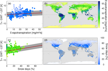
Figure 3 Evapotranspiration (ET) and snow influence the offset ΔT between groundwater temperature (GWT) and land surface temperature (LST). (a) The influence of ET on ΔT. Color coding shows the percentage of snow days at each measurement point (figure 3(d)). The red line gives the fitted offset  . The 95% prediction interval (for 0% snow days) is given in grey. (b) Global map of ET. (c) The influence of snow on ΔT. Color coding shows the corresponding ET (figure 3(b)). The red line gives the fitted offset
  , in grey the 95% prediction interval (for 0 mg m−2 s−1 ET). (d) Global map of the percentage of snow days.
Download figure:
Standard image High-resolution imageFigure 3(c) and figure S8(b) depict the influence of surface snow cover on the offset between GWT and LST. The data show that the percentage of snow days increases annual mean GWTs and therefore raises the offset  .
.
The best fit is obtained by the following solution:
The half width of the confidence interval is given as the uncertainty. The RMSE of the fit is 1.4 K. Figures 3(a) and (c) display  and
and  separately, and a surface plot of
  is given in figure S9. This fit implies an increase in the offset of 0.035 ± 0.002 K per mg m2 s−1 of ET and an increase of 0.066 ± 0.003 K for each percent in snow days. The determined
  is added to LST to estimate GWTs for all analyzed measurement points (figure 2(b), figure S10). As expected, GWTs from urban areas such as the data from Mikkeli, Finland (table S1, figure S11(e)) are severely underestimated, on average by 3.8 K, as heat flux from buildings has to be considered as well (Benz et al 2016) for an accurate estimation. Additionally, measured GWTs in (semi-)arid regions with only minor ET, such as the Lower Jordan Valley (figure S11(b)), are on average 2.3 K lower than estimated GWTs. Here irrigation is assumed to be the main source of recharge (Zemann et al 2014). In spite of these local discrepancies, estimated and measured GWT agree well. While they correlate the same as LST and GWT (Pearson correlation coefficient: 0.97), R2 increases by 0.05 to 0.95, and the RMSE (1.4 K) is improved by 0.5 K compared to the one between GWT and LST.
By applying this method to global datasets of decadal mean evapotranspiration and snow days (figures 3(b) and 3(d)), a global map of the expected offset was created (figure 4(a)). It ranges from 0 K in the arid regions such as Northern Africa, the Arabian Peninsula and central Australia to more than 6 K in the polar regions. However, with no available measurement points in such high latitudes, further research is needed to validate these findings. The average half-width of the 95% prediction interval is 2.76 ± 0.03 K (figure S12). By adding the estimated offset to the measured LSTs, shallow global groundwater temperature is estimated (figure 4(b)).

Figure 4 (a) Estimated offset between land surface temperatures (LST) and shallow groundwater temperatures (GWT). Shown are the total offset  as well as the individual offsets caused by evapotranspiration (
 ) and snow cover (
 ). (b) Estimated shallow GWTs.
Download figure:
Standard image High-resolution image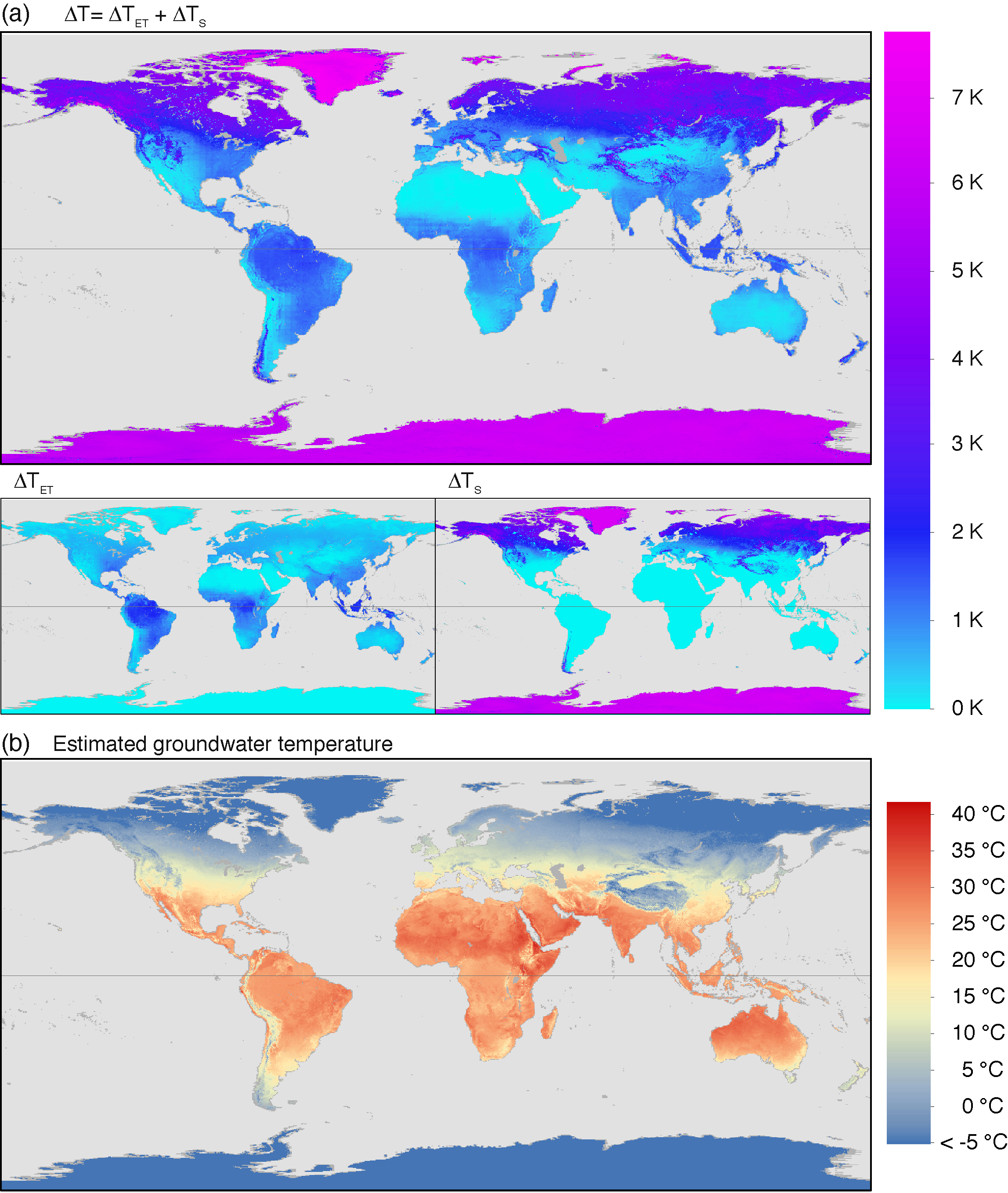
4. Conclusion
The main focus of this study was on the global scale offset between 10 year mean groundwater temperatures (GWT) and satellite-derived land surface temperatures (LST). A total of 2 548 shallow GWT measurement points in 29 countries and two overseas territories are utilized to analyze the offset  . We find that GWTs are warmer than LST in 83% of all measurement points. The average offset is 1.2 ± 1.5 K with highest differences between GWT and LST in both the warmest and coldest areas of Earth. These high offsets are linked to evapotranspiration, which alters the latent heat flow and therefore surface energy balance, and snow cover, which insulates warm GWTs during the winter. We are able to quantify the influence from ET and snow cover and to describe the global offset between GWT and LST as a superposition of both effects. Hence, global shallow groundwater temperatures can be estimated using only satellite-derived data. However, it is important to note that groundwater flow is not yet considered. A previous study by Benz et al (2016) found that, on a city scale, the Pearson correlation coefficient between GWT and LST can be increased by 6% to 10%, if groundwater flow is scrutinized. Additionally, GWT anomalies caused by other regional effects such as geothermal hotspots, fossil groundwater and subsurface urban heat islands cannot be resolved with the presented method. Still, the proposed estimation technique provides shallow global GWTs with a RMSE of only 1.4 K and a coefficient of determination R2 of 0.95.
Additionally, the found link between the offset, snow cover and evapotranspiration can be applied to future climate scenarios. With above ground temperatures rising due to climate change (IPCC 2013) GWTs are expected to increase as well. However, climate change also impacts snow cover and evapotranspiration and we can therefore assume that GWTs will increase at a different rate than LSTs. In areas where snow cover is decreasing, our results imply that the offset between GWT and LST will decrease and GWT will increase at a slower rate than LST. In areas where the offset is predominantly dictated by evapotranspiration (ET), declining ET will decrease the offset and thus reduce GWT increase, whereas rising ET will increase the offset and thus amplify the overall GWT increase.
Acknowledgments
The financial support for SA Benz from the German Research Foundation (DFG) under grant number BL 1015/4-1 and the Swiss National Science Foundation (SNSF) under grant number 200021L 144288 is gratefully acknowledged. Additionally we would like to thank Tanja Liesch, Anna Ender, Moritz Zemann, Julian Xanke, Tobias Kling, and Elisabeth Eiche (KIT), Erich Fischer (BMLFUW, Austria), Susanne Reimer (Tiefbauamt Karlsruhe), Michael Kramel (Geo_t, Germany), Stefan Terzer (IAEA), Jean Michel Lemieux (Université Laval), Dr Hussein Abed Jassas (GEOSURV, Iraq), Teppo Arola (Golder), Harold Wilson Tumwitike Mapoma (China University of Geosciences; University of Malawi), Mauricio Muñoz (Andean Geothermal Centre of Excelence, Chile), Yuliya Vystavna (OM Beketov National University of Urban Economy at Kharkiv, Ukraine), and Martina Maisch (LUBW, Germany) for their information and groundwater temperature data. We acknowledge support by Deutsche Forschungsgemeinschaft and Open Access Publishing Fund of Karlsruhe Institute of Technology. Finally, we would like thank the two anonymous reviewers for their helpful comments.
Input data and results (3.4 GB) are made available in the supplementary material.
An extensive list of all GWT sources can be found in table S1. All Code written for Google Earth Engine is available and can be run to generate all data under the following URLs (google account needed):
LST: https://code.earthengine.google.com/4a1bc64dbc3351a1e364490758d4cf2d.
ET: https://code.earthengine.google.com/cf262aa371c68704c5b059d574498510.
Snow days: https://code.earthengine.google.com/82cca1edb8f025027ef1e7b7573f16e3.