
Topic models with elements of neural networks: investigation of stability, coherence, and determining the optimal number of topics
- Published
- Accepted
- Received
- Academic Editor
- Davide Chicco
- Subject Areas
- Data Mining and Machine Learning, Data Science, Natural Language and Speech, Text Mining, Neural Networks
- Keywords
- Topic modeling, Neural topic models, Stability, Coherence, Optimal number of topics, Renyi entropy, Word embeddings
- Copyright
- © 2024 Koltcov et al.
- Licence
- This is an open access article distributed under the terms of the Creative Commons Attribution License, which permits unrestricted use, distribution, reproduction and adaptation in any medium and for any purpose provided that it is properly attributed. For attribution, the original author(s), title, publication source (PeerJ Computer Science) and either DOI or URL of the article must be cited.
- Cite this article
- 2024. Topic models with elements of neural networks: investigation of stability, coherence, and determining the optimal number of topics. PeerJ Computer Science 10:e1758 https://doi.org/10.7717/peerj-cs.1758
Abstract
Topic modeling is a widely used instrument for the analysis of large text collections. In the last few years, neural topic models and models with word embeddings have been proposed to increase the quality of topic solutions. However, these models were not extensively tested in terms of stability and interpretability. Moreover, the question of selecting the number of topics (a model parameter) remains a challenging task. We aim to partially fill this gap by testing four well-known and available to a wide range of users topic models such as the embedded topic model (ETM), Gaussian Softmax distribution model (GSM), Wasserstein autoencoders with Dirichlet prior (W-LDA), and Wasserstein autoencoders with Gaussian Mixture prior (WTM-GMM). We demonstrate that W-LDA, WTM-GMM, and GSM possess poor stability that complicates their application in practice. ETM model with additionally trained embeddings demonstrates high coherence and rather good stability for large datasets, but the question of the number of topics remains unsolved for this model. We also propose a new topic model based on granulated sampling with word embeddings (GLDAW), demonstrating the highest stability and good coherence compared to other considered models. Moreover, the optimal number of topics in a dataset can be determined for this model.
Introduction
Topic modeling is widely used in various areas that require big data clustering, especially when analyzing text collections. In practice, however, many topic models generate uninterpretable topics that require users to measure the coherence of the model. Moreover, many topic models possess a certain level of semantic instability, which means that different runs of the algorithm on the same source data lead to different solutions, and this problem is still open. Furthermore, not for every model, it is possible to determine the correct number of topics in a dataset. However, the model parameter ‘number of topics’, which determines the level of granularity of the cluster solution, has to be set manually in an explicit form. Recent research (Koltcov et al., 2021; Koltcov et al., 2020) has shown that models supporting an automatic setting of the number of topics perform poorly and depend on other hidden parameters, for example, the concentration parameter. Nevertheless, using domain knowledge, for example, word embeddings or combinations of neural network layers, seems promising in solving the above problems. Currently, several topic models with neural network elements have been proposed. However, systematic research of such models in terms of quality measures, such as interpretability and stability, and the possibility of determining the correct number of topics, was not conducted. Commonly, researchers concentrate only on interpretability ignoring the problems of stability and the problem of the number of topics. The tuning of topic models is usually based on empirical criteria, which have not been tested on labeled datasets. Thus, the main goal of this work is to fill this gap partially and to test four well-known and available to a wide range of users neural topic models such as (1) embedded topic model (ETM) (Dieng, Ruiz & Blei, 2020), (2) Gaussian Softmax distribution (GSM) model (Miao, Grefenstette & Blunsom, 2017), (3) Wasserstein autoencoders with Dirichlet prior (W-LDA) (Nan et al., 2019), and (4) Wasserstein autoencoders with Gaussian Mixture prior (WTM-GMM) (https://zll17.github.io/2020/11/17/Introduction-to-Neural-Topic-Models/#WTM-GMM). Moreover, we propose and test a new topic model called a granulated topic model with word embeddings (GLDAW). To test the models, we consider three labeled test datasets and two levels of their pre-processing. Also, we investigate the influence of six different word embeddings (three in Russian and three in English) on ETM and GLDAW models. To estimate the different features of the models, we calculate three measures: coherence, stability, and Renyi entropy.
To simplify the structure of this work, an overview of topic models with elements of neural networks is provided in Appendix A. An overview of different types of word embeddings is presented in Appendix B. Let us note that word embeddings have become an important tool in the field of natural language processing (NLP) allowing translation of text data into numeric vectors that can be further processed by various algorithms.
The rest of our work consists of the following parts. ‘Measures in the field of topic modeling’ describes measures that we use to estimate models under study. ‘Granulated topic model with word embeddings’ describes the new proposed granulated model with word embeddings. This model is an extension of the ‘granulated topic model’ (Koltcov et al., 2016a), which additionally incorporates a semantic context contained in word embeddings. ‘Computational experiments’ contains the description of the datasets and types of used word embeddings and outlines the design of our computer experiments for each of the considered models. ‘Results’ describes the results of computer experiments for each model in terms of the chosen quality measures. ‘Discussion’ compares the obtained results for each model. ‘Conclusions’ summarizes our findings.
Measures in the field of topic modeling
To estimate considered topic models, we focus on three measures that reflect different model properties: coherence, stability, and Renyi entropy. An extensive overview of different quality measures in the field of topic modeling can be found in works Rüdiger et al. (2022) and Chauhan & Shah (2021). Below, each of the chosen measures is described in more detail.
Coherence
Coherence allows one to evaluate the consistency of the model, i.e., how often the most probable words of a topic co-occur in the documents. In other words, it evaluates how strongly the words in the topic are related to each other. Thus, coherence reflects the interpretability of the inferred topics. We have used the “u_mass” version of the coherence measure. This measure can be expressed as follows (Mimno et al., 2011): is a list of M most probable words in topic t, D(v) is the number of documents containing word v, and D(v, v′) is the number of documents where words v and v′ co-occur. Thus, coherence is the sum of logs of the ratio of the number of documents with two co-occurring words to the total number of documents with one of the two evaluated words. In other words, if there are highly probabilistic words in a topic, that have a high co-occurrence in highly probabilistic documents, coherence is large, and the topic is well interpretable. In our numerical experiments, we use Gensim library for the calculation of coherence (Rehurek & Sojka, 2010).
Stability
Prior to defining the stability of a topic model, it is necessary to define the similarity of two topics. We use the definition proposed in Koltcov, Koltsova & Nikolenko (2014). The computation of similarity is based on the normalized Kullback–Leibler divergence: where Max is the maximum value of symmetric Kullback–Leibler divergence, K is symmetric Kullback–Leibler divergence, which is expressed as for topics t1 and t2, ϕ⋅t1 is the probability distribution of words in the first topic, ϕ⋅t2 is the probability distribution of words in the second topic. As demonstrated in Koltcov, Koltsova & Nikolenko (2014), two topics can be considered semantically similar if Kn > 90%, meaning that the most probable 50–100 words of these topics are the same. In our work, a topic is considered stable if it is reproduced in three runs of the model with the same number of topics and normalized Kullback–Leibler divergence is not less than 90%. Then, the number of such stable topics is counted. This number depends on the model architecture, the total number of topics, which is a model parameter, and the type of used word embeddings. Therefore, in our experiments, we varied these factors.
Renyi entropy
The complete derivation of Renyi entropy can be found in Koltcov (2017) and Koltcov (2018). In this article, we give the basic idea behind the deformed Renyi entropy for determining the optimal number of topics. The matrix of distribution of words in topics is one of the results of topic modeling. In practice, researchers work with the most probable words in every topic. These highly probabilistic words can be used to compute the following quantities: (1) Density-of-states function, ρ = N/(WT), where N is the number of words with high probabilities, W is the number of words in the vocabulary, and T is the number of topics. We define “high probability” as a probability larger than 1/W. (2) Energy of the system , where the summation is over all highly probabilistic words and all topics. Renyi entropy can be expressed as follows: where the deformation parameter q = 1/T is the inverse number of topics (Koltcov, 2018). Since entropy can be expressed in terms of information of the statical system (S = -I (Beck, 2009)), a large value of deformed entropy corresponds to a small amount of information and vice versa. Due to the fact that the set of highly probabilistic words in different topic solutions changes with a variation in the total number of topics and other model hyperparameters, Koltcov, Ignatenko & Koltsova (2019) and Koltcov et al. (2020) discovered the following. First, a small number of topics leads to a very large Renyi entropy, meaning that such a model is poor in terms of information. Second, a significant increase in the number of topics leads to a large entropy as well because topic modeling generates solutions with almost uniform distributions, i.e., topics are indistinguishable. Therefore, the information of such a system is small as well. Experiments have shown that Renyi entropy has a minimum at a certain number of topics, which depends on the particular dataset. Moreover, experiments on labeled datasets have shown that this minimum corresponds to the number of topics obtained with manual labeling. Thus, Renyi entropy can be used to determine the optimal number of topics. It should be noted that this approach is suitable for the datasets with a “flat topic structure” and for the datasets with a hierarchical structure (Koltcov et al., 2021).
Granulated topic model with word embeddings
Before describing our proposed topic model, it is necessary to introduce basic notations and assumptions. Let D be a collection of documents, and let be the set of all words (vocabulary). Each document d is represented as a set of words w1, ...wnd, . The key assumption of probabilistic topic models is that each word w in a document d is associated with some topic , and the set of such topics is finite. Further, the set of documents is treated as a collection of random independent samples (wi, di, zi), i = 1 ..n, from a discrete distribution p(w, d, z) on the finite probability space . Words and documents are observable variables, and the topic of every word occurrence is a hidden variable. In topic models, documents are represented as bags of words, disregarding the order of words in a document and the order of documents in the collection. The basic assumption here is that specific words occurring in a document depend only on the corresponding topic occurrences and not on the document itself. Thus, it is supposed that p(w|d) can be represented as p(w|d) = p(w|t)p(t|d) = ϕwtθtd, where ϕwt = p(w|t) is the distribution of words by topics and θtd = p(t|d) is the distribution of topics by documents. Therefore, to train a topic model on a set of documents means to find the set of topics , and more precisely, to find the distributions and θtd, d ∈ D. Let us denote by matrix Φ = {ϕwt} the set of distributions of words by topics and by matrix Θ = {θtd} the set of distributions of topics in the documents. There are two major approaches to finding Φ and Θ. The first approach is based on an algorithm with expectation–maximization inference. The second approach is based on an algorithm that calculates probabilities via the Monte-Carlo method. A detailed description of the models and types of inferences can be found in the recent reviews of topic models (Helan & Sultani, 2023; Chauhan & Shah, 2021).
Granulated latent Dirichlet allocation model
The granulated topic model is based on the following ideas. First, there is a dependency between a pair of unique words, but unlike the convolved Dirichlet regularizer model (Newman, Bonilla & Buntine, 2011), this dependency is not presented as a predefined matrix. Instead, it is assumed that a topic consists of words that are not only described by a Dirichlet distribution but also often occur together; that is, we assume that words that are characteristic for the same topic are often collocated inside some relatively small window (Koltcov et al., 2016a). That means all words inside a window belong to one topic or a small set of topics. As previously described in Koltcov et al. (2016a), each document can be treated as a grain surface consisting of granules, which, in turn, are represented as sequences of subsequent words of some fixed length. The idea is that neighboring words usually are associated with the same topic, which means that topics in a document are not distributed independently but rather as grains of words belonging to the same topic.
In general, the Gibbs sampling algorithm for local density of the distribution of words in topics can be formulated as follows:
-
Matrices Θ and Φ are initialized.
-
Loop on the number of iterations
-
For each document d ∈ D repeat |d| times:
-
sample an anchor word wj ∈ d uniformly at random
-
sample its topic t as in Gibbs sampling (Griffiths & Steyvers, 2004)
-
set ti = t for all i such that |i − j| ≤ l, where l is a predefined window size.
-
-
In the last part of the modeling, after the end of sampling, the matrices Φ and Θ are computed from the values of the counters. Thus, the local density function of words in topics and the size of the window work as a regularization. The main advantage of this model is that it has very high stability and outperforms other models such as ARTM (Vorontsov, 2014), LDA (E-M algorithm) (Blei, Ng & Jordan, 2003), LDA with Gibbs sampling algorithm (Griffiths & Steyvers, 2004) and pLSA (Hofmann, 1999) in terms of stability (Koltcov et al., 2016b).
Granulated latent Dirichlet allocation with word embeddings
A significant disadvantage of the GLDA model is that the Renyi entropy approach for determining the number of topics is not accurate for this model (Koltcov, 2018). In this work, we propose a new granulated model (GLDAW), which takes into account information from word embeddings. The GLDAW model is realized with Gibbs sampling algorithm as follows. There are three stages of the algorithm. In the first stage, we form a matrix of the nearest words by given word embeddings. At this stage, the algorithm checks if the vocabularies of the dataset and word embeddings match. If a word from the given set of word embeddings is missing from the dataset’s vocabulary, then its embedding is deleted. This procedure reduces the size of the set of word embeddings and speeds up the computation at the second stage. Then, the matrix of the nearest words in terms of their embedding vectors is built. The number of the nearest words is set manually by the “window” parameter. In fact, this parameter is analogous to the “window” parameter in GLDA.
In the second stage, the computation is similar to Granulated LDA Gibbs sampling with the choice of an anchor word from the text and the attachment of this word to a topic. The topic is computed based on the counters. However, unlike the granulated version, where the counters of the nearest words (to the current anchor word) in the text were increased, this algorithm increases the counters of the words corresponding to the nearest embeddings. Thus, running through all the documents and all the words, we create the matrix of the counters of words taking into account their embeddings.
In the third stage, the resulting matrix of counters is used to compute the probabilities of all words as in the standard LDA Gibbs sampling: , , where nwt equals how many times word w appeared in topic t, nt is the total number of words assigned to topic t, ntd equals how many times topic t appeared in document d. Thus, this procedure of sampling resembles the standard LDA Gibbs sampling, for which the Renyi entropy approach works accurately, but it also has the features of granulated sampling leading to the high stability of the model. It should be noted that the proposed sampling does not have any artificial assumptions about the distribution of topics, as in ‘Embedded topic model’ (Dieng, Ruiz & Blei, 2020), for example, where the topics are sampled from a categorical distribution with parameters equal to the dot product of the word and topic vectors. The proposed sampling procedure uses only information about the closeness of word embeddings.
Computational experiments
A short description of the models (ETM, GSM, W-LDA, WTM-GMM, and GLDAW) used in computational experiments is given in Table 1. For a more detailed description of the models, we refer the reader to Appendix A.
| Model | Short description | Word embeddings |
|---|---|---|
| ETM | A log-linear model that takes the inner product of the word embedding matrix (ρ) and the topic embedding (αk): proportions of topics θd ∼ LN(0, I) (LN means logistic-normal distribution), topics zdn ∼ Cat(θd) (Cat means categorical distribution), words wdn ∼ softmax(ρTαzdn). The architecture of the model is a variational autoencoder. | yes |
| GSM | Proportions of topics (θd) are set with Gaussian softmax, topics zdn ∼ Multi(θd) (Multi refers to the multinomial distribution), words wdn ∼ Multi(βzdn) (βzdn is the distribution of words in topic zdn.) The architecture of the model is a variational autoencoder. | no |
| W-LDA | The prior distribution of the latent vectors z is set as Dirichlet distribution, while the variational distribution is regulated under the Wasserstein distance. The architecture is a Wasserstein autoencoder. | no |
| WTM-GMM | An improved model of the original W-LDA. The prior distribution is set as Gaussian mixture distribution. The architecture is a Wasserstein autoencoder. | no |
| GLDAW | It is assumed that words in a topic not only follow Dirichlet distribution but also that the words with near embeddings often co-occur together. The inference is based on Gibbs sampling. | yes |
To test the above models, the following datasets were used:
-
The ‘Lenta’ dataset is a set of 8,630 news documents in Russian language with 23,297 unique words. The documents are manually marked up into 10 classes. However, some of the topics are close to each other and, therefore, this dataset can be described by 7–10 topics.
-
The ‘20 Newsgroups’ dataset is a collection of 15,425 news articles in English language with 50,965 unique words. The documents are marked up into 20 topic groups. According to Basu, Davidson & Wagstaff (2008), 14–20 topics can describe the documents of this dataset, since some of the topics can be merged.
-
The ‘WoS’ dataset is a class-balanced dataset, which contains 11,967 abstracts of published papers available from the Web of Science. The vocabulary of the dataset contains 36,488 unique words. This dataset has a hierarchical markup, where the first level contains seven categories, and the second level consists of 33 areas.
The datasets with lemmatized texts used in our experiments are available at https://doi.org/10.5281/zenodo.8407610. For experiments with Lenta dataset we have used the following Russian-language embeddings: (1) Navec are compact Russian embeddings (the part of “Natasha project” https://github.com/natasha/navec), (2) 300_wiki embeddings are fastText embeddings for Russian language(https://fasttext.cc/docs/en/pretrained-vectors.html, Bojanowski et al., 2017), (3) Rus_vectors embeddings (RusVectores project) are available at https://rusvectores.org/en/. For experiments with 20 Newsgroups and WoS datasets, we have used the following English-language embeddings: (1) Crawl-300d-2M (fastText technology), available at https://fasttext.cc/docs/en/english-vectors.html (Mikolov et al., 2018), (2) Enwiki_20180420_win10_100d are word2vec embeddings(https://pypi.org/project/wikipedia2vec/0.2/, version 0.2) (Yamada et al., 2016) (3) wiki_news_300d-1M are fastText embeddings (https://fasttext.cc/docs/en/english-vectors.html (Mikolov et al., 2018)).
Numerical experiments were carried out as follows. Every dataset has gone through two levels of pre-processing. At the first level, the words consisting of three or fewer letters were removed. At the second level, additionally, the words that appear less than five times were removed. Thus, the size of Lenta dataset after the first stage of pre-processing is 17,555 unique words and after the second stage of pre-processing is 11,225 unique words. The size of 20 Newsgroups dataset is 41,165 and 40,749 unique words, correspondingly. The size of WoS dataset is 31,725 and 14,526 unique words for two levels of pre-processing. For two types of pre-processing, the experiments have been carried out separately.
For the ETM and GLDAW models, three Russian-language and three English-language word embeddings were used. In the ETM model, pre-trained word embeddings can be trained additionally during the process of modeling. Therefore, this model was tested with and without additional training of word embeddings. The window size for GLDAW model was varied as follows: 10, 50, and 100 for Lenta and 20 Newsgroups datasets; 10, 30, and 50 for WoS dataset.
The number of topics was varied in the range [2; 50] in increments of one topic for all models. All three chosen measures were calculated as a mean of three runs of each model. Source codes of our computational experiments are available at https://doi.org/10.5281/zenodo.8410811.
Results
Numerical results are described according to the chosen measures. So, in the first part, we describe the results of all five models in terms of coherence. The second part analyzes the stability of the models. In the third part, we assess the possibility of determining the true number of topics. Finally, in the fourth part, we present the computational speed of each model on an example of WoS dataset.
Results on coherence
As discussed, the ETM model was trained according to two schemes: (1) with pre-trained word embeddings and (2) with additionally trained embeddings. Figure 1 demonstrates the results of ETM model with different types of word embeddings in terms of coherence measure. Let us note that for some numbers of topics, there is no coherence value for pre-trained embeddings on the first level of pre-processing for WoS dataset, which means that the model performs poorly with these settings.
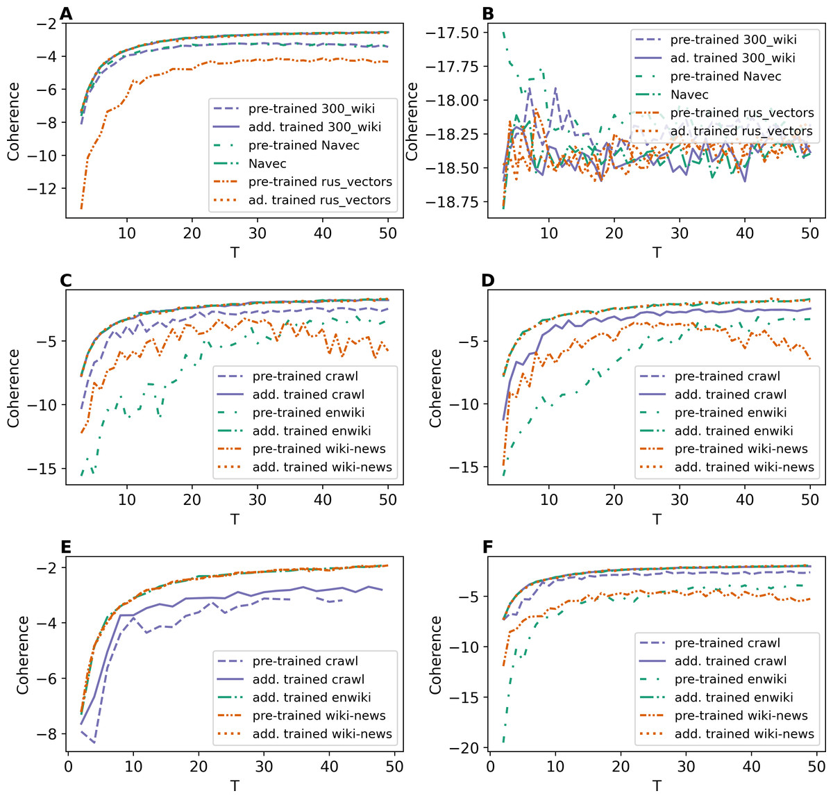
Figure 1: Dependence of coherence on the number of topics (ETM model).
(A) Lenta dataset: first level of pre-proccessing. (B) Lenta dataset: second level of pre-proccessing. (C) 20 Newsgroups dataset: first level of pre-processing. (D) 20 Newsgroups dataset: second level of pre-processing. (E) WoS dataset: first level of pre-processing. (F) WoS dataset: second level of pre-processing.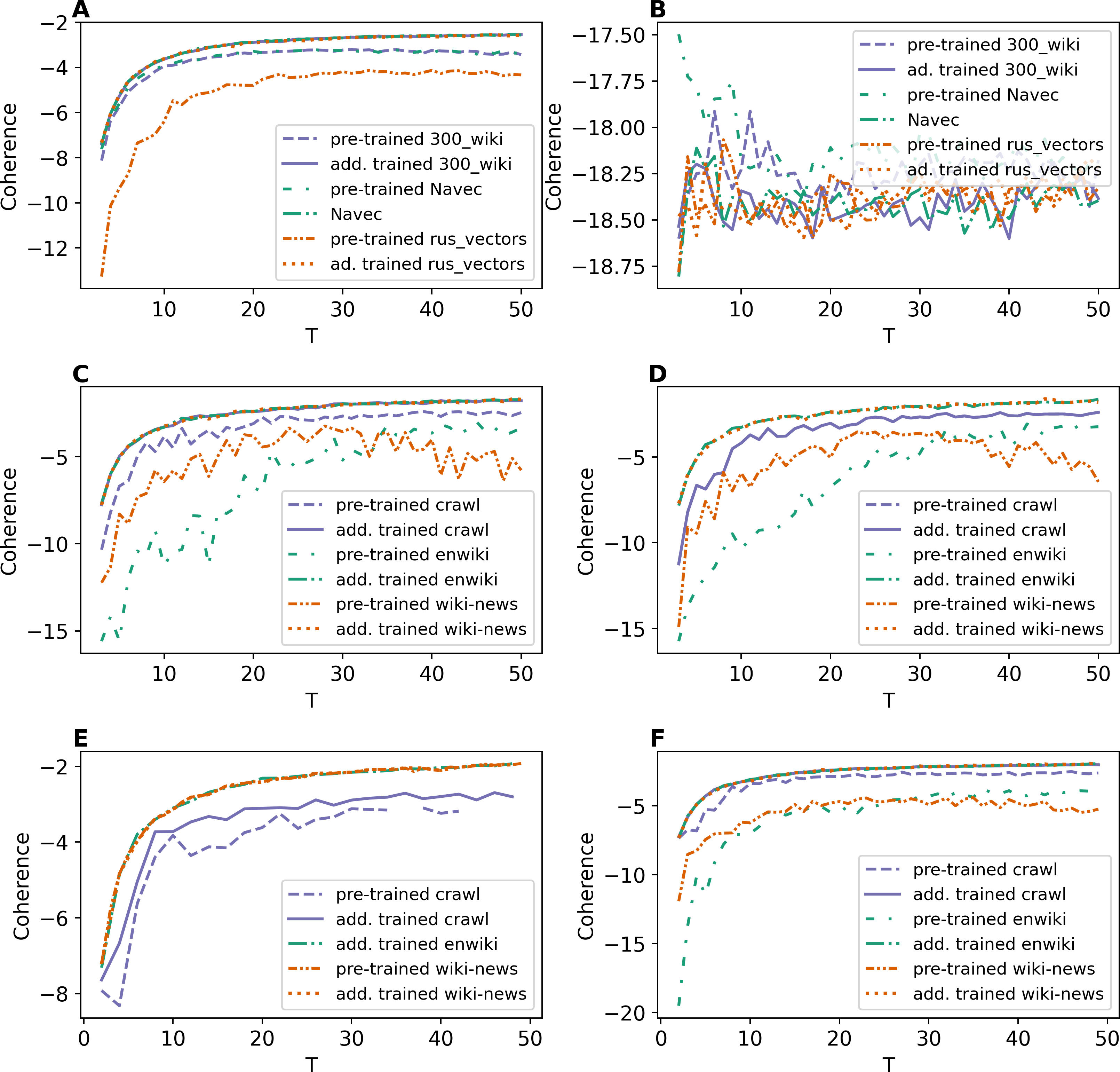
Based on our results (Fig. 1), one can conclude the following. First, training embeddings during the model learning leads to better coherence for all three datasets. Moreover, in this case, the coherence values are almost identical for different types of embeddings for each dataset. Second, ETM model performs poorly on a small dataset (11–12 thousand words) with strong pre-processing (Fig. 1B). Therefore, larger datasets should be used for ETM model to get better quality. Third, the behavior of the coherence measure does not allow us to estimate the optimal number of topics for this model.
Let us note that the GSM, W-LDA and WTM-GMM models do not use word embeddings. The results for these three topic models are given in Fig. 2. Overall, our results demonstrate that the dataset pre-processing does not strongly influence the output of the above models. The GSM model performs worse than the other models, while WTM-GMM shows the best results. However, the fluctuation of coherence is larger for all these models than for ETM model.
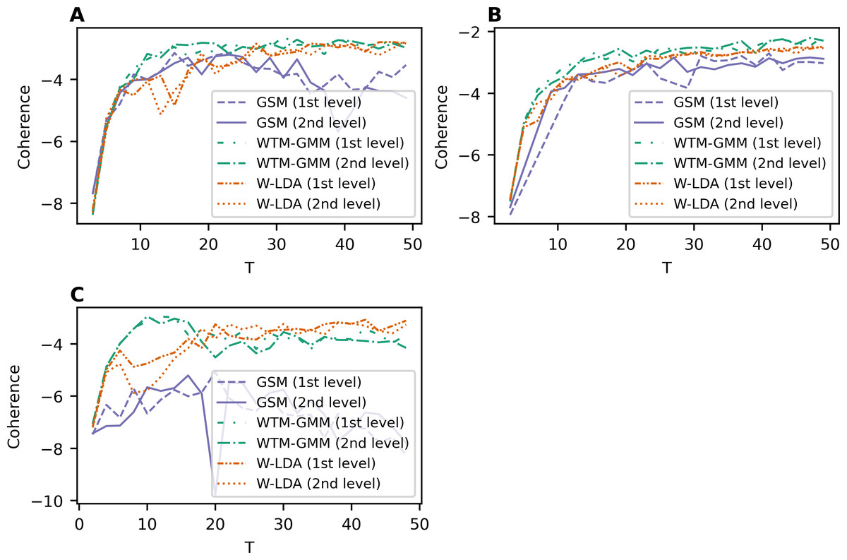
Figure 2: Dependence of coherence on the number of topics (W-LDA, WTM-GMM, and GSM models).
(A) Lenta dataset. (B) 20 Newsgroups dataset. (C) WoS dataset.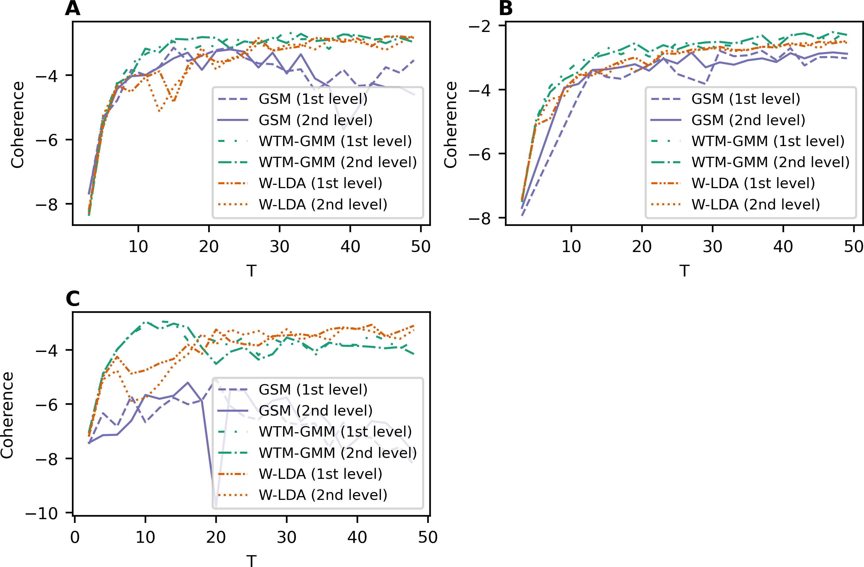
Figure 3 demonstrates the results of GLDAW model. Figures 3A and 3B show that pre-processing of Lenta dataset does not have a strong influence on the performance of this model. Besides that, the coherence values do not depend on the type of embeddings. The fluctuation for different embeddings is about 0.1, while for W-LDA, WTM-GMM, and GSM models, the fluctuation is about 1. The fluctuation of the coherence value of ETM model for trained embeddings is also about 0.1. The values of coherence for the 20 Newsgroups dataset are given in Figs. 3C and 3D. The fluctuation of coherence values for all types of embeddings is about 0.4 on the first level of pre-processing and about 0.3 on the second level of pre-processing. For the WoS dataset (Figs. 3E, 3F), the fluctuation of coherence for all types of embeddings is about 0.3 for T < 25 and about 0.5 for T > 25 on the first level of pre-processing. On the second level of pre-processing, the fluctuation of coherence does not exceed 0.3. Thus, the GLDAW model has a smaller fluctuation of coherence in comparison to considered neural topic models. Also, the quality almost does not depend on the size of the window. The ETM model has a similar fluctuation value, but it does not perform well for the deeply pre-processed small datasets, while the GLDAW performance is good for both levels of pre-processing.
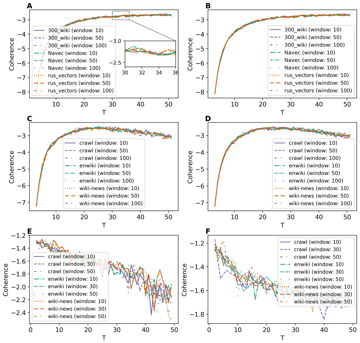
Figure 3: Dependence of coherence on the number of topics (GLDAW model).
(A) Lenta dataset: first level of pre-proccessing. (B) Lenta dataset: second level of pre-proccessing. (C) 20 Newsgroups dataset: first level of pre-processing. (D) 20 Newsgroups dataset: second level of pre-processing. (E) WoS dataset: first level of pre-processing. (F) WoS dataset: second level of pre-processing.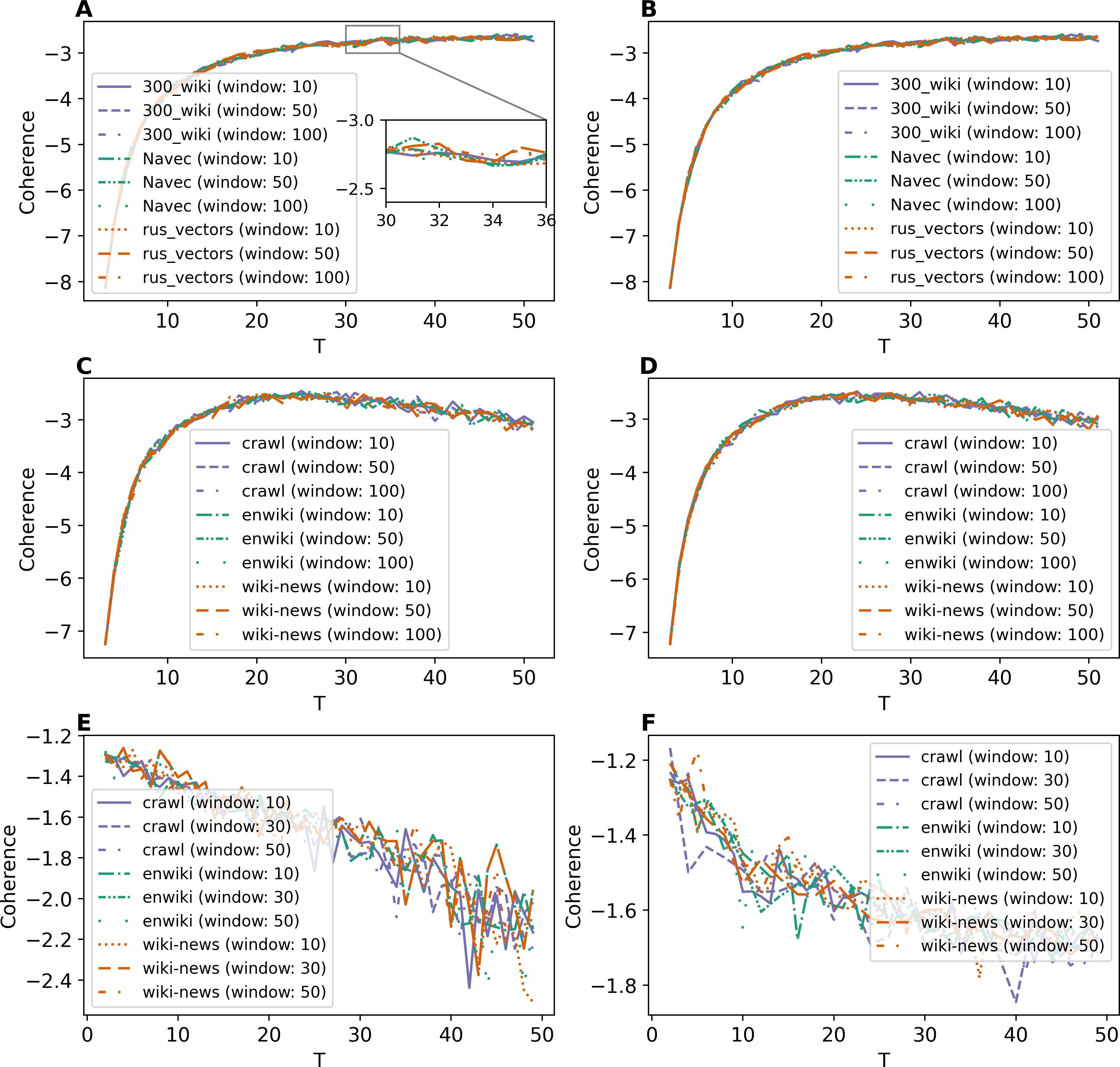
To compare all five models, Fig. 4A demonstrates the best coherence values for Lenta dataset. ETM model shows the best quality with Navec embeddings at the first level of pre-processing. However, this model does not perform well on the second level of pre-processing (Fig. 1C). The GLDAW model has the second-best result with values of 0.1 less than ETM but performs well on the second level of pre-processing. Besides that, the GLDAW model does not require the additional training of embeddings, unlike the ETM model.
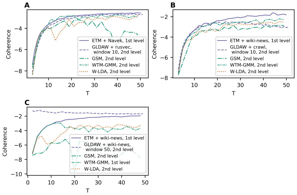
Figure 4: Dependence of the best coherence values on the number of topics.
(A) Lenta dataset. (B) 20 Newsgroups dataset. (C) WoS dataset.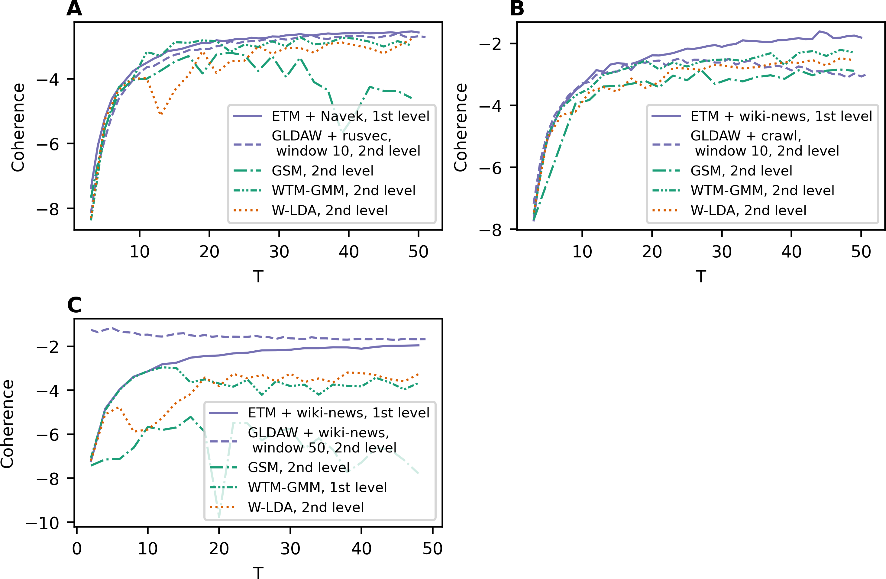
The best models in terms of coherence for 20 Newsgroups dataset are presented in Fig. 4B. The best result is achieved by ETM as well. The GLDAW model outperforms W-LDA in the range of 2–20 topics, while W-LDA outperforms GLDAW in the range of 30–50 topics. It should be noted that the optimal number of topics is 14–20 for this dataset, according to human judgment. Figure 4C demonstrates the best results for the WoS dataset. GLDAW outperforms other models in terms of coherence, while the ETM model has the second-best results for this dataset.
Results on stability
Let us remind that stability was computed based on the three runs of every model with the same settings. The topic is considered stable if it is reproduced in all runs with a normalized Kullback–Leibler divergence above 90%. Otherwise, the topic is considered unstable. The number of stable topics was calculated for topic solutions with a fixed total number of topics. Figures 5–7 demonstrate the number of stable topics vs. the total number of topics in topic solutions. Since the calculation of stability is a very time-consuming procedure, we considered only T = 10, 20, 30 for WoS dataset.
Figures 5A and 5B demonstrate the results on the number of stable topics for Lenta dataset. One can see that additional training of word embeddings significantly improves the model stability for a large number of topics. However, for a small number of topics, the difference is insignificant. On average, “rus_vectors” embeddings demonstrate the best result. Let us note that the stability measure based on Kullback–Leibler divergence does not allow us to determine the optimal number of topics for Lenta dataset.
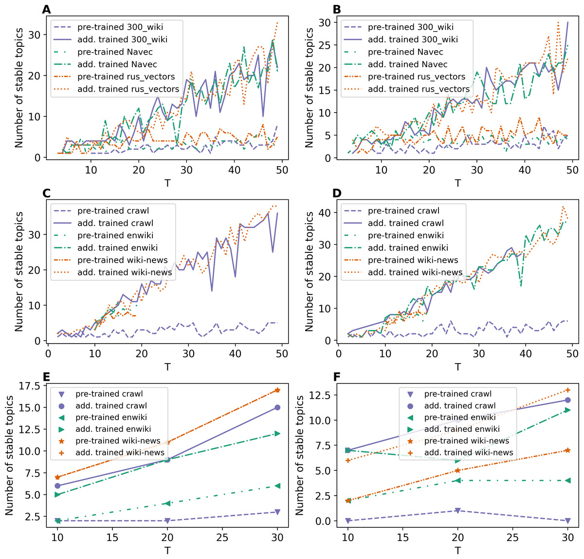
Figure 5: Dependence of the number of stable topics on the total number of topics (ETM model).
(A) Lenta dataset: first level of pre-proccessing. (B) Lenta dataset: second level of pre-proccessing. (C) 20 Newsgroups dataset: first level of pre-processing. (D) 20 Newsgroups dataset: second level of pre-processing. (E) WoS dataset: first level of pre-proccessing. (F) WoS dataset: second level of pre-proccessing.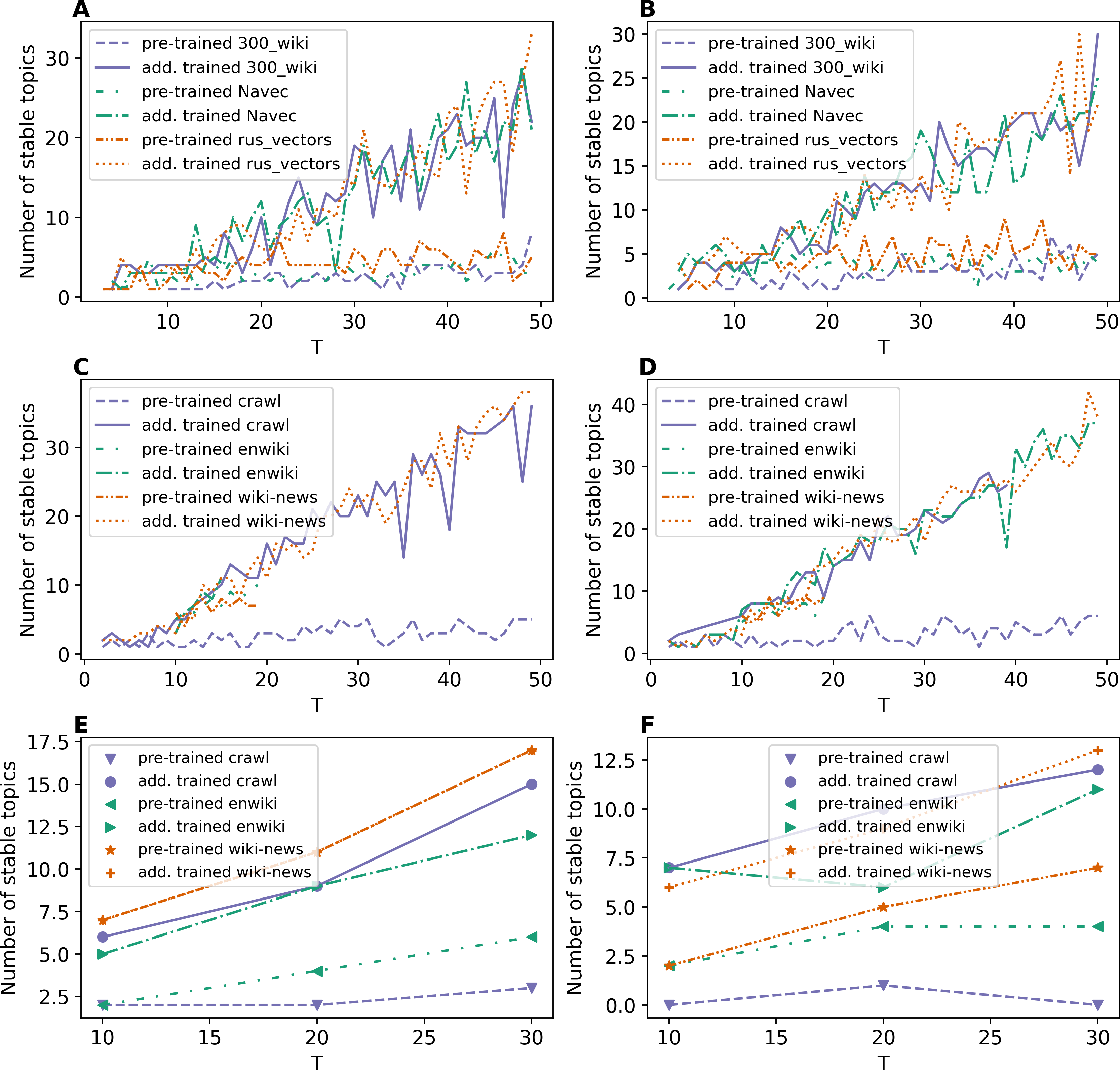
Figures 5C and 5D demonstrate the results on stability for the 20 Newsgroups dataset. One can see that the application of pre-trained embeddings leads to less stable models as well as for the Lenta dataset. For example, the models with wiki-news-300d-1 M and enwiki_20180420 embeddings are stable only in the range of 10–20 topics on the first level of pre-processing. The second level of pre-processing increases stability, and the fluctuation of stability reduces. Also, it should be noted that these curves do not allow us to evaluate the optimal number of topics for 20 Newsgroups dataset. Altogether, we obtain the following results for the above two datasets: for Lenta dataset, ETM model is stable in the range of 1–4 topics, while this dataset has 7–10 topics according to human judgment; for 20 Newsgroups dataset, ETM model is stable in the range of 8–15 topics while this dataset has 14–20 topics according to human judgment.
Figures 5E and 5F demonstrate the results on stability for the WoS dataset. Again, one can see that additional training of embeddings increases the stability of the model. Moreover, one can see that the ETM model is sensitive to the type of word embeddings and may produce a relatively large number of stable topics that are not present in the dataset according to human judgment.
Figure 6 demonstrates the results on stability for the W-LDA, WTM-GMM and GSM models. The level of pre-processing does not affect the stability of these models. However, the stability level of the GSM, W-LDA, and WTM-GMM models is 3–4 times less than the stability of ETM. The GSM model demonstrates the worst results in terms of stability for the 20 Newsgroups dataset. It starts to produce stable solutions only beginning with 10 topics, and in general, it has 3–6 times worse stability than the WTM-GMM and W-LDA models. Let us note that for the WoS dataset, we obtained zero stable topics for most cases. On the whole, all models are stable in the range of 1–3 topics for Lenta dataset and in the range of 9–15 topics for the 20 Newsgroups dataset. However, for the WoS dataset we obtained the worst results without stable topics for the GSM and W-LDA models.
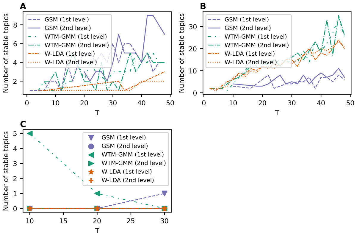
Figure 6: Dependence of the number of stable topics on the total number of topics (W-LDA, WTM-GMM and GSM models).
(A) Lenta dataset. (B) 20 Newsgroups dataset. (C) WoS dataset.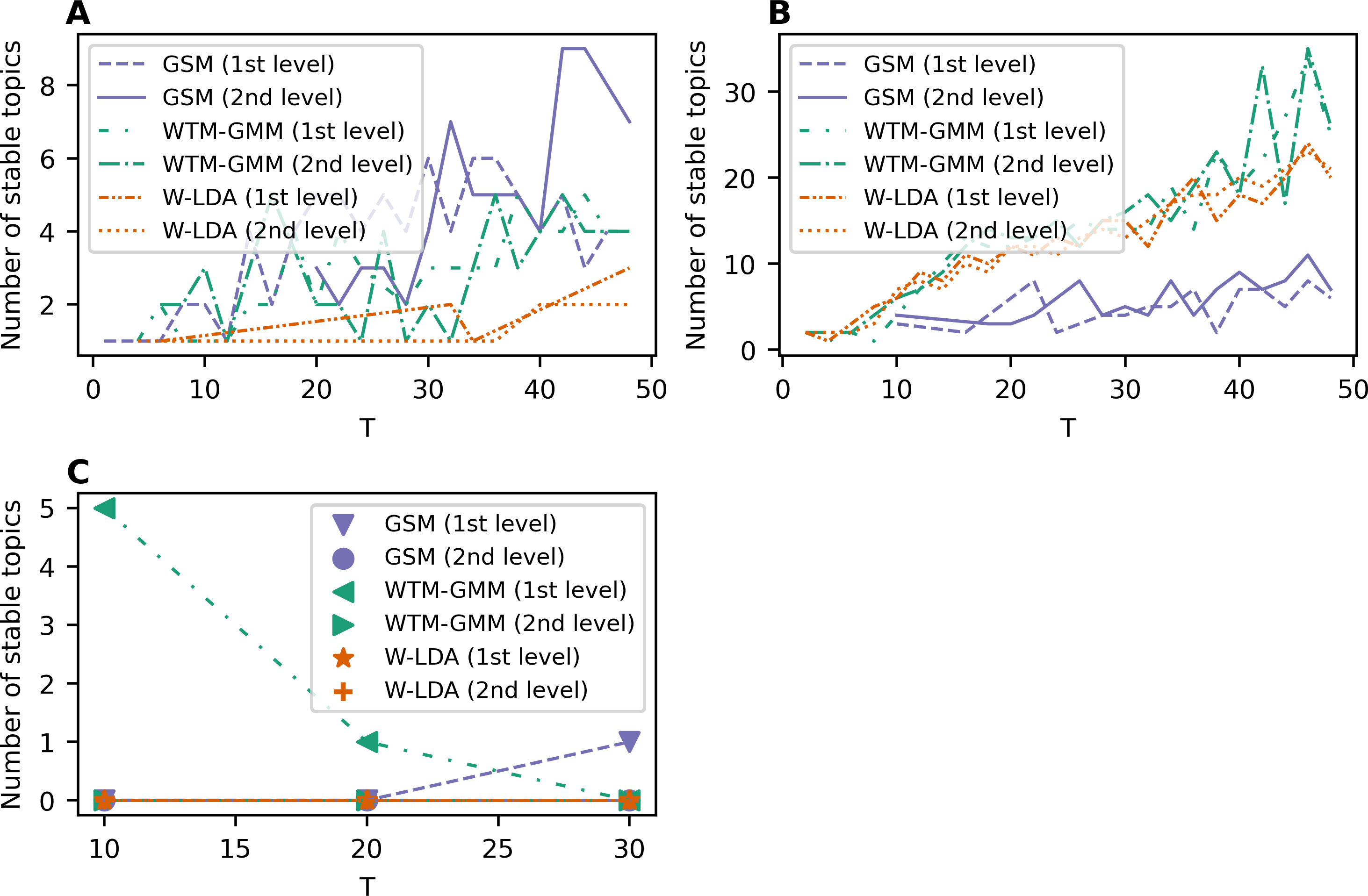
Figures 7A and 7B demonstrate results on stability for GLDAW model on Lenta dataset. The levels of pre-processing almost do not influence the results. The number of stable topics is about 6–8 topics for solutions on 7–10 topics for both levels of pre-processing. The further increase in the number of topics leads to a small increase in the number of stable topics up to 16 topics. Figures 7C and 7D show the results for the 20 Newsgroups dataset. These curves show that the levels of pre-processing do not influence the stability either. Moreover, the fluctuation of stability is significantly smaller in the region of the optimal number of topics than in the region of a large number of topics. Furthermore, the largest number of stable topics that the GLDAW model produces is about 27 topics when increasing the number of topics. Thus, the GLDAW model does not prone to produce redundant topics, while the ETM model with 50 topics produces 35 stable topics meaning that it finds redundant topics (since the real number of topics is 14–20). At the same time, the GLDAW model produces 14–18 stable topics in this range. Figures 7E and 7F demonstrate the results on stability for WoS dataset. The number of stable topics varies in the range of 4–11 topics, which is close to the number of topics on the first level of markup. On the whole, the GLDAW model demonstrates the best result in terms of stability among all considered models and for all three datasets. Since this model does not depend significantly on the type of embeddings and is not sensitive to the window size, we recommend using a window size equal to ten in order to speed up the calculation time.
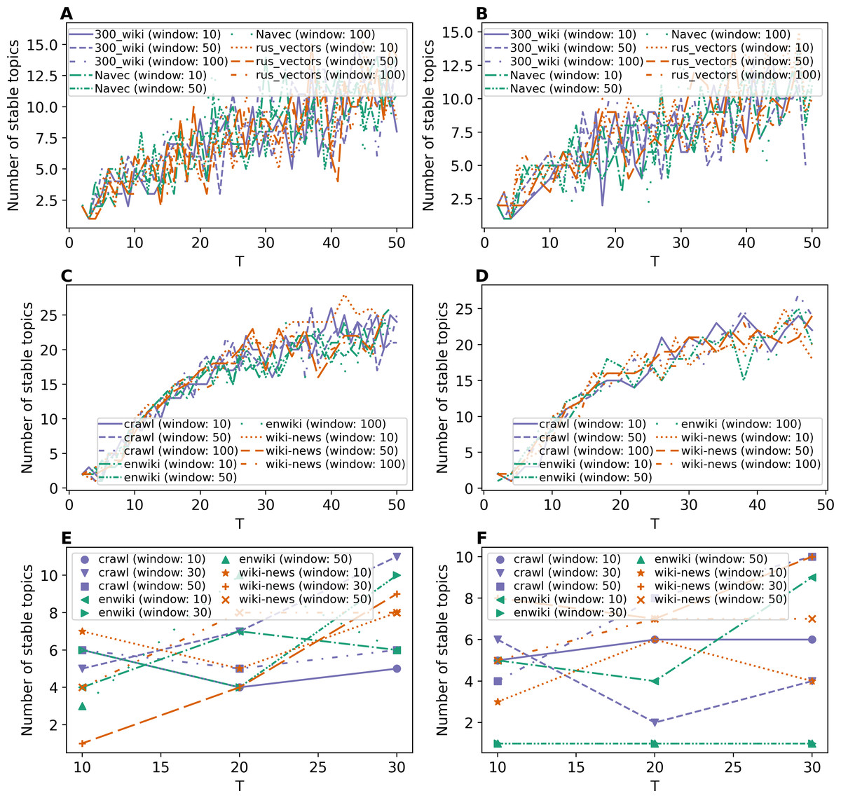
Figure 7: Dependence of the number of stable topics on the total number of topics (GLDAW model).
(A) Lenta dataset: first level of pre-proccessing. (B) Lenta dataset: second level of pre-proccessing. (C) 20 Newsgroups dataset: first level of pre-processing. (D) 20 Newsgroups dataset: second level of pre-processing. (E) WoS dataset: first level of pre-proccessing. (F) WoS dataset: second level of pre-proccessing.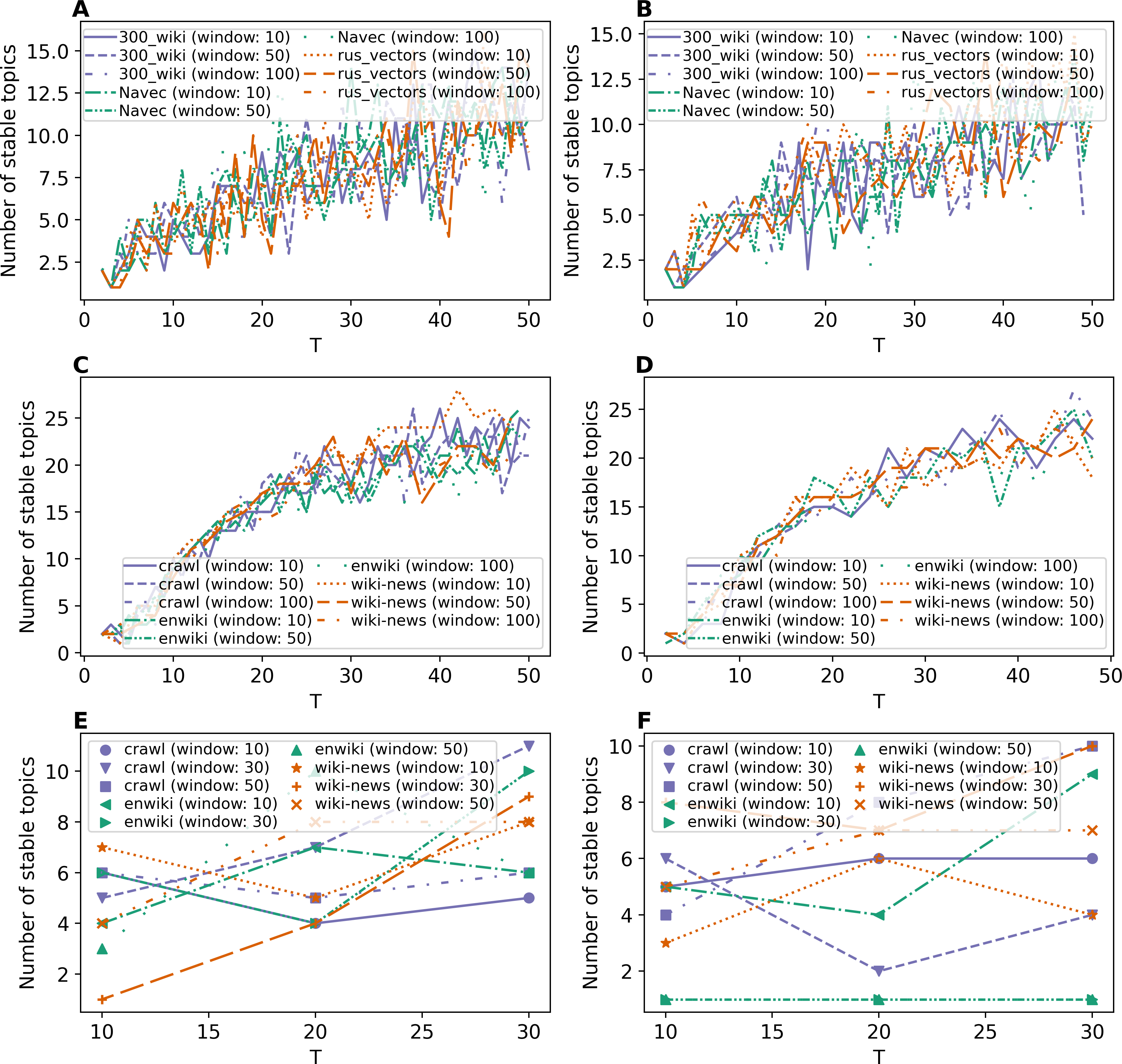
Results on Renyi entropy
Various studies of topic models (Koltcov, 2018; Koltcov et al., 2020; Koltcov et al., 2021) have shown that the number of topics corresponding to the minimal Renyi entropy equals the optimal number of topics, i.e., the number of topics according to human judgment. There can be several minimal points in the case of hierarchical structure (Koltcov et al., 2021). However, in this work, we focus on labeled datasets with a flat structure leading to a single Renyi entropy minimum, and for hierarchical WoS dataset, we consider only the markup on the first level containing categories.
Figures 8A and 8B demonstrate Renyi entropy curves for ETM model on Lenta dataset. First, the figures show that applying pre-trained embeddings results in a minimum occurring at a small number of topics, about 4–6 topics, that does not match the human labeling. Second, additionally trained embeddings shift the minimum in the range of 9–10 topics. Besides that, the difference between models with different embeddings is insignificant. Third, the pre-processing almost does not influence the curves for models with additionally trained embeddings.
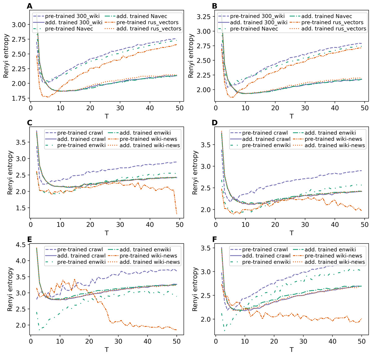
Figure 8: Dependence of Renyi entropy on the number of topics (ETM model).
(A) Lenta dataset: first level of pre-proccessing. (B) Lenta dataset: second level of pre-proccessing. (C) 20 Newsgroups dataset: first level of pre-processing. (D) 20 Newsgroups dataset: second level of pre-processing. (E) WoS dataset: first level of pre-processing. (F) WoS dataset: second level of pre-processing.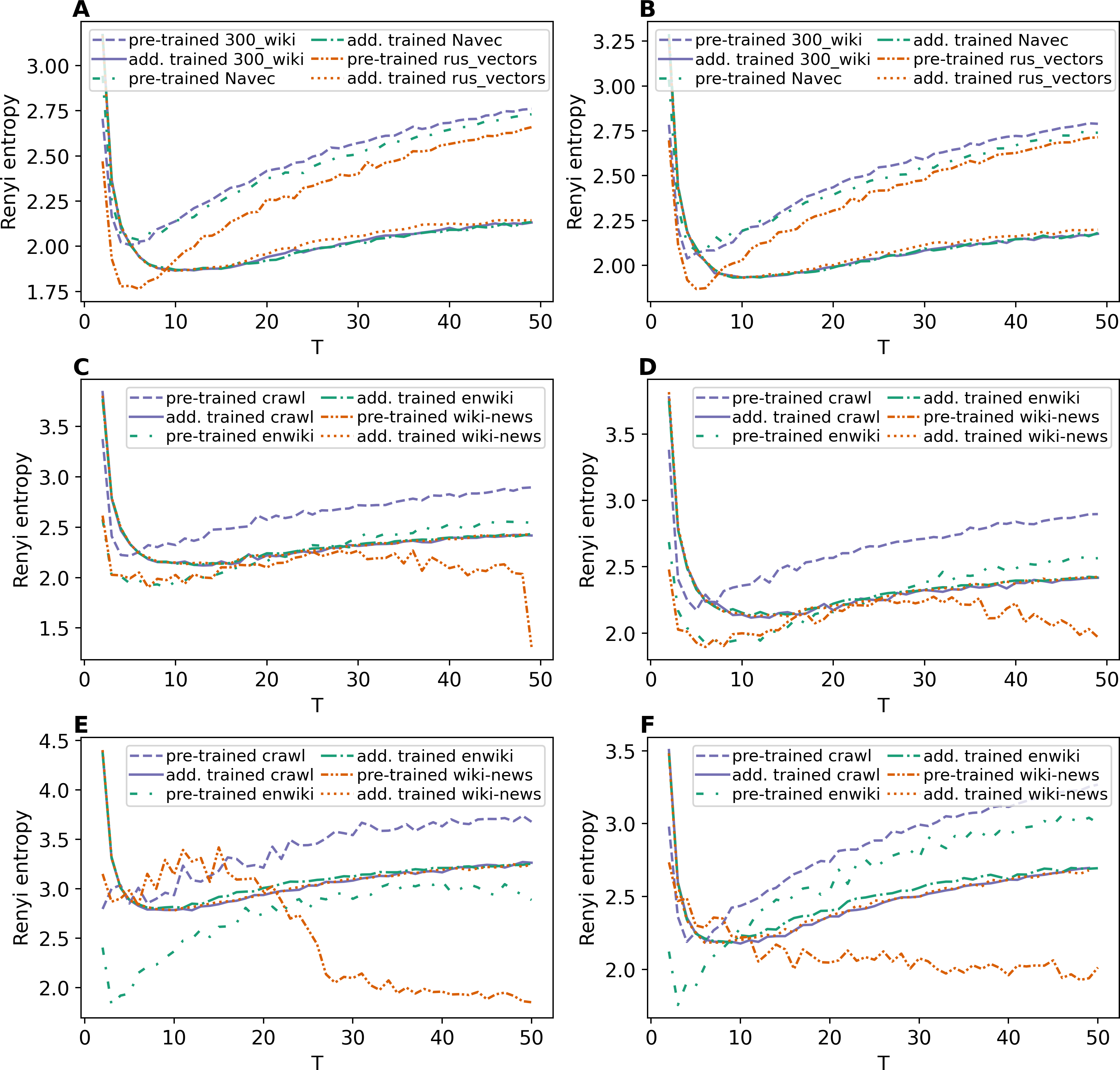
Renyi entropy curves for ETM model on the 20 Newsgroups dataset are given in Figs. 8C and 8D. These figures show that it is necessary to train embeddings. There is no significant difference between models with different embeddings. The minimum of Renyi entropy is at 11 topics, which does not match the human mark-up.
Figures 8E and 8F demonstrate Renyi entropy curves for the ETM model on the WoS dataset. The curves corresponding to pre-trained embeddings have minimum points not matching the mark-up (2–3 topics for the first level of pre-processing and 3–6 topics for the second level of pre-processing). The minimum of Renyi entropy for additionally trained embeddings corresponds to 8–12 topics. Let us note that this number is the same for both pre-processing levels and all three datasets, meaning that sampling from the categorical distribution parameterized by the dot product of the word and topic embeddings works as a too strong regularization. It leads to the fact that different datasets’ results do not differ much. Therefore, Renyi entropy cannot be used to determine the optimal number of topics for ETM model.
Renyi entropy curves for the neural topic models trained on Lenta dataset are given in Fig. 9A. The results show that Renyi entropy for W-LDA and GSM models does not depend on the level of pre-processing. The entropy minima for GSM and W-LDA models do not correspond to the optimal number of topics. However, Renyi entropy minimum (six topics) for the WTM-GMM model on the second level of pre-processing almost corresponds to the true number of topics. The results on Renyi entropy for the 20 Newsgroups dataset are given in Fig. 9B. This figure shows that the levels of pre-processing do not influence the entropy values. The minimum for GSM model is at eight topics; for W-LDA is at 12 topics; and for WTM-GMM is at 42 topics. Figure 9C demonstrates corresponding results for the WoS dataset. One can see that again, the pre-processing levels do not significantly influence the entropy values. The minimum for the GSM model is at 12-16 topics; for W-LDA is at 4-6 topics; and for WTM-GMM is at six topics. Thus, Renyi entropy minimum for WTM-GMM model is very close to the true number of topics. However, for GSM and W-LDA, the entropy minima do not correspond to the optimal number of topics. Thus, we can conclude that Renyi entropy cannot be used to determine the optimal number of topics for these models.
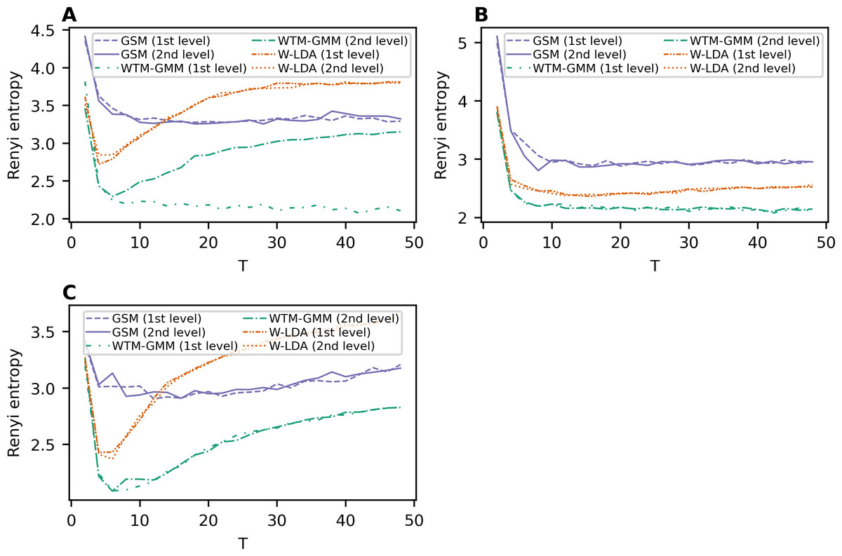
Figure 9: Dependence of Renyi entropy on the number of topics (W-LDA, WTM-GMM and GSM models).
(A) Lenta dataset. (B) 20 Newsgroups dataset. (C) WoS dataset.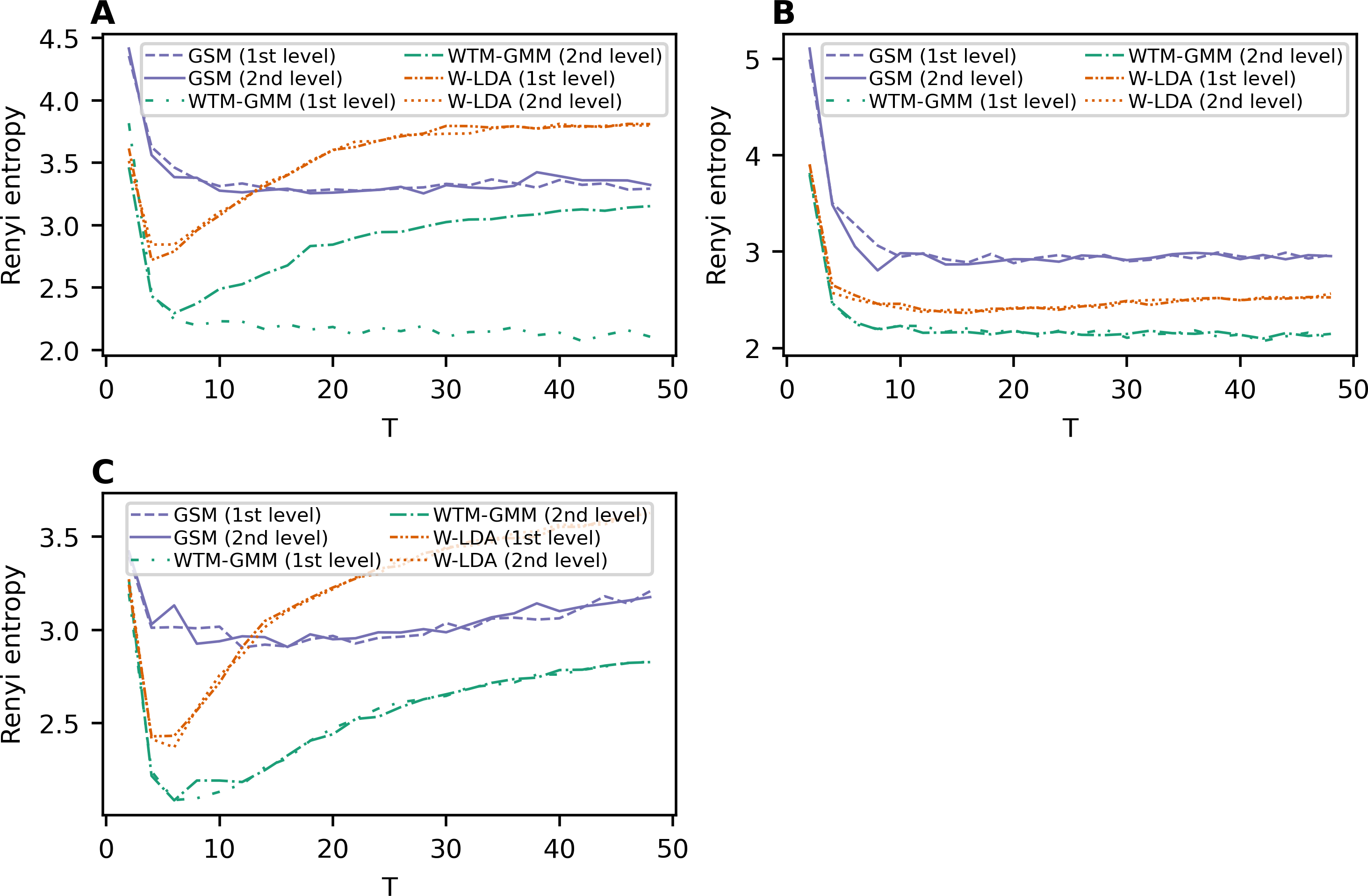
The Renyi entropy curves for the GLDAW model trained on Lenta dataset are presented in Figs. 10A and 10B. The computations show that the GLDAW model has Renyi entropy minimum in the range of 7–9 topics, and different types of embeddings do not change positions of the minimum. This result matches the number of topics according to the human mark-up. Figures 10C and 10D demonstrate Renyi entropy curves for the 20 Newsgroups dataset. The minimum of Renyi entropy is located in the range of 15-17 topics, which also matches human judgment. Figures 10E and 10F demonstrate Renyi entropy curves for the WoS dataset. The Renyi entropy minimum is achieved in the range of 11–13 topics, and different types of embeddings do not change the position of the minimum. This result is close to the number of topics achieved according to the human mark-up.
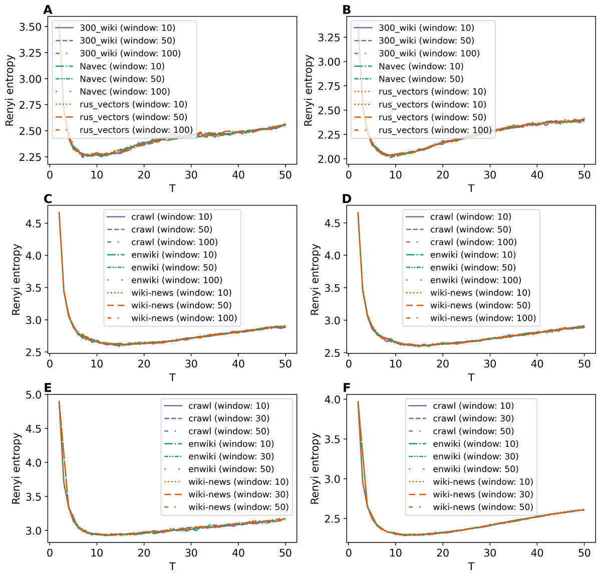
Figure 10: Dependence of Renyi entropy on the number of topics (GLDAW model).
(A) Lenta dataset: first level of pre-proccessing. (B) Lenta dataset: second level of pre-proccessing. (C) 20 Newsgroups dataset: first level of pre-processing. (D) 20 Newsgroups dataset: second level of pre-processing. (E) WoS dataset: first level of pre-processing. (F) WoS dataset: second level of pre-processing.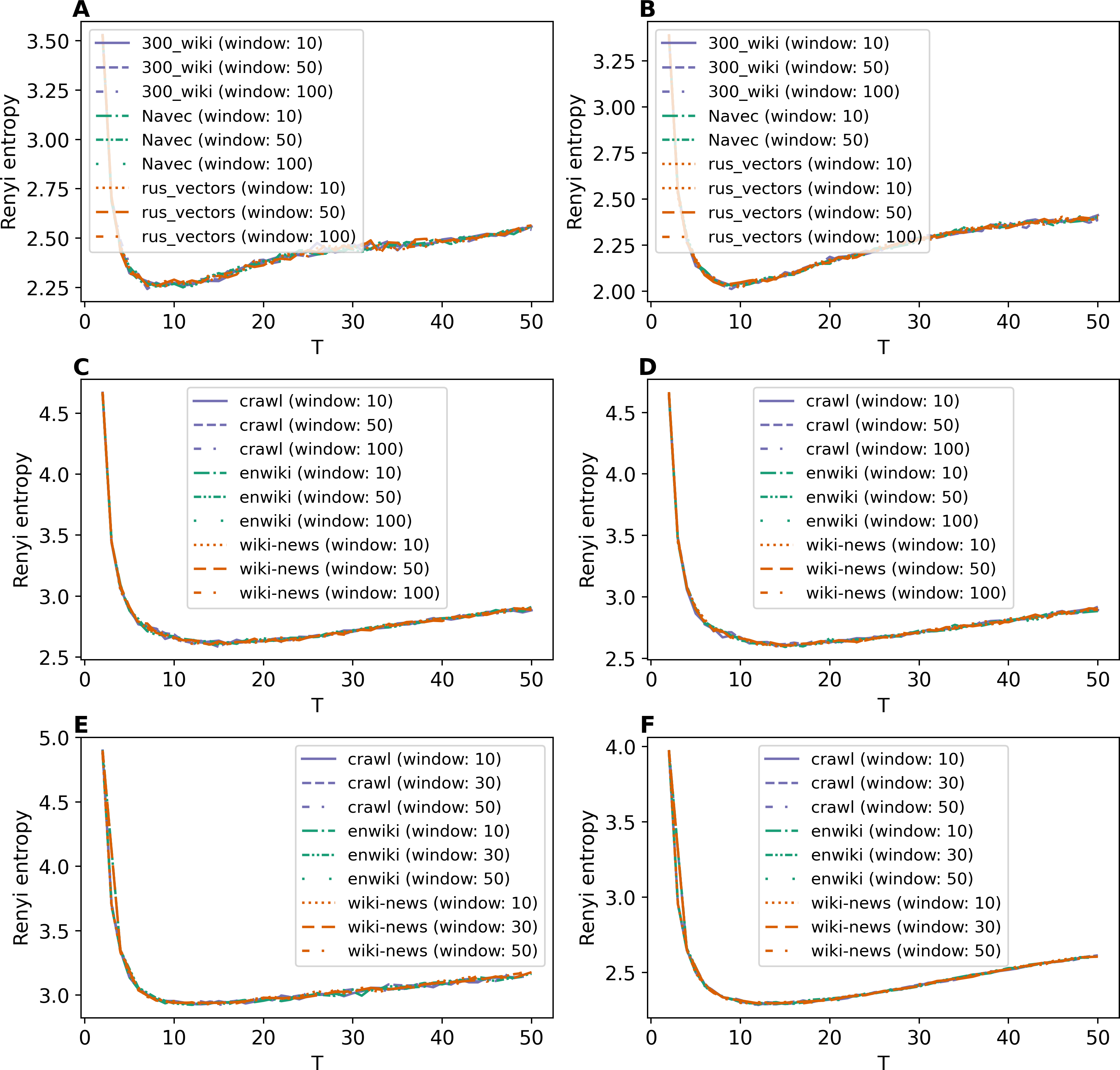
Thus, we can conclude that, first, the GLDAW model almost does not depend on the embedding type and window size for both Russian-language and English-language embeddings. Second, this model allows us to correctly determine the approximation of the optimal number of topics for all three datasets.
Computational speed
Table 2 demonstrates the computational speed of the considered models on an example of WoS dataset with the second level of pre-processing for different values of the total number of topics, namely, for T = 10, 20, 30. The number of epochs for W-LDA, WTM-GMM, GSM, and ETM was fixed at 300, and the number of iterations for GLDAW model was also fixed at 300. All calculations were performed on the following equipment: computer with Intel Core i7-12700H 2.7 GHz, Ram 16 Gb, operation system: Windows 10 (64 bits), graphics card: NVIDIA GeForce RTX 3060. Let us note that the W-LDA, WTM-GMM, GSM, and ETM models were computed with the application of CUDA while the GLDAW model was not optimized for parallel computing.
| Model | Number of topics | Calculation time |
|---|---|---|
| ETM with pre-trained embeddings (enwiki) | 10 | 248.25 sec |
| ETM with pre-trained embeddings (enwiki) | 20 | 257.62 sec |
| ETM with pre-trained embeddings (enwiki) | 30 | 260.32 sec |
| ETM with additionally trained embeddings (enwiki) | 10 | 250.60 s |
| ETM with additionally trained embeddings (enwiki) | 20 | 261.80 sec |
| ETM with additionally trained embeddings (enwiki) | 30 | 266.94 sec |
| GSM | 10 | 5422.5 sec |
| GSM | 20 | 6696.0 sec |
| GSM | 30 | 6717.0 sec |
| W-LDA | 10 | 6640.0 sec |
| W-LDA | 20 | 6760.6 sec |
| W-LDA | 30 | 6905.9 sec |
| WTM-GMM | 10 | 8299.7 sec |
| WTM-GMM | 20 | 9340.5 sec |
| WTM-GMM | 30 | 9340.8 sec |
| GLDAW with enwiki embeddings, window size 50 | 10 | 41.49 sec |
| GLDAW with enwiki embeddings, window size 50 | 20 | 47.23 sec |
| GLDAW with enwiki embeddings, window size 50 | 30 | 53.44 sec |
Based on the presented time costs, one can see that the proposed GLDAW model is the fastest model among the considered ones and, thus, can be recommended for practical use.
Discussion
Comparison of models in terms of coherence
Our calculations demonstrated that ETM model has both positive and negative properties in terms of coherence. First, it is necessary to train embeddings for both Russian-language and English-language embeddings to obtain good quality for this model. The procedure of additional training of embeddings is time-consuming, but, in this case, the coherence value is the largest among all considered models for the Lenta and 20 Newsgroups datasets. Second, ETM model performs poorly on datasets with 11,000 words or less. This means that this model is not suitable for small datasets. Moreover, additional training of embeddings does not improve the coherence of the topic model for small datasets.
The GLDAW model has slightly worse results than the ETM model in terms of coherence for the Lenta and 20 Newsgroups datasets; however, it demonstrates the best result for WoS dataset. In addition, this model does not require additional training of embeddings and does not depend on the window size. Moreover, the GLDAW model performs well on small and large datasets, meaning that this model can be used in a wide range of tasks.
The GSM, WTM-GMM, and W-LDA models perform worse than ETM with trained embeddings and GLDAW in terms of coherence. Moreover, these models have significant fluctuations of the coherence measure under variation of the number of topics. The GSM model demonstrates the worst results in terms of coherence for all three datasets.
Stability of topic models
The best result of the ETM model with trained embeddings in terms of stability for Lenta dataset is about 4–5 topics for topic solutions on 10 topics. For topic solutions on 50 topics, this model has about 27–30 stable topics. The ETM model with untrained embeddings has only 5–7 stable topics for solutions on 50 topics. Therefore, additional training of word embeddings is required for this model. For the 20 Newsgroups dataset, the results on stability are as follows. The ETM model with untrained embedding demonstrates a limited level of stability for some types of embeddings. For example, for wiki-news-300d-1M and enwiki_20180420 embeddings, the model has stable topics only in the region of 10–20 topics; in other cases, most topics were not reproduced in all three runs. The models with trained embeddings perform better in terms of stability. There are 27–37 stable topics for solutions on 50 topics and 12–15 stable topics (depending on the type of embeddings) for solutions on 20 topics. For the WoS dataset, we can also observe that ETM model with additionally trained embeddings produces a larger number of stable topics, namely, 5–7 stable topics for T = 10, 6–11 stable topics for T = 20, and 12–17 stable topics for T = 30 for both levels of pre-processing.
For the Lenta dataset, the GLDAW model has 7–8 stable topics for solutions on 10 topics outperforming the ETM model. Moreover, it has 8–16 stable topics for solutions on 50 topics, meaning that it is less prone to see redundant topics in this dataset than ETM model, which produces about 30 stable topics. For the 20 Newsgroups dataset, GLDAW model demonstrates the best result in the range of 15–19 topics, which is slightly better than the ETM model with trained embeddings. For topic solutions on 50 topics, GLDAW model has 22–25 stable topics. For WoS dataset, the GLDAW model has 4–11 stable topics for the considered values of T, which is close to the human markup. Thus, the GLDAW model outperforms all other models in terms of stability, showing the best stability for the number of topics close to the optimal one, while for the ETM model, the number of stable topics increases as the number of topics increases; what does not match the human mark-up.
The stability of GSM, W-LDA, and WTM-GMM is worse than that of ETM and GLDAW. WTM-GMM shows the best results (among the neural topic models), producing three stable topics for solutions on 10 topics for the Lenta dataset, 13 stable topics for solutions on 20 topics for the 20 Newsgroups dataset, and five stable topics for solutions on 10 topics for the WoS dataset. GSM model demonstrates the worst result in terms of stability.
Determining the optimal number of topics
ETM model with trained embeddings has a minimum Renyi entropy at 10–11 topics for the Russian-language dataset as well as for the English-language datasets. Thus, the Renyi entropy approach does not allow us to differentiate between datasets for this model and, therefore, to find the optimal number of topics. It happens due to the procedure of sampling. The sampling is made from a categorical distribution parametrized by embeddings, meaning that embeddings have a greater impact on topic solutions than the dataset itself.
The GLDAW model has a minimum Renyi entropy at 7–9 topics for the Lenta dataset, 15–17 topics for the 20 Newsgroups dataset, and 11–13 topics for the WoS dataset, which is close to the human labeling results. Besides that, our computations show that the type of embeddings does not influence the entropy curve behavior for this model. Finally, the GSM, WTM-GMM, and W-LDA models have a minimum entropy for 4–6 topics for the Russian-language dataset, and a fluctuating minimum at 14–42 topics for 20 Newsgroups dataset. For the WoS dataset, the WTM-GMM model has a minimum for 6 topics, GSM model demonstrates a minimum for 12–16 topics, and W-LDA has a minimum for 4–6 topics.
Thus, according to our results, we can conclude the following. The GLDAW model is the best among all considered models based on the combination of three measures. It has a slightly smaller coherence value than the ETM model for two of three datasets but the largest stability in the region of the optimal number of topics. Moreover, this granulated model allows us to determine the optimal number of topics more accurately than the other models. In addition, this model is the fastest in terms of computational cost among the considered ones.
Conclusions
In this work, we have investigated five topic models (ETM, GLDAW, GSM, WTM-GMM, and W-LDA) with elements of neural networks. One of these models, namely the GLDAW model, is new and is based on the granulated procedure of sampling, where a set of nearest words is found according to word embeddings. For the first time, all models were evaluated simultaneously in terms of three measures: coherence, stability, and Renyi entropy. We used three datasets with two levels of pre-processing as benchmarks: the Russian-language dataset ‘Lenta’, the English-language ‘20 Newsgroups’ and ‘WoS’ datasets. The experiments demonstrate that the ETM model is the best model in terms of coherence for two of three datasets, while the GLDAW model takes second place for those two datasets and first place for the third dataset. At the same time, the GLDAW model has higher stability than the ETM model. Besides that, it is possible to determine the optimal number of topics in datasets for the GLDAW model, while the ETM model is unable for that. In addition, the GLDAW model demonstrates the smallest computational cost among the considered models. The GSM, WTM-GMM, and W-LDA models demonstrate worse results than the ETM and GLDAW models in terms of all three measures. Thus, the proposed GLDAW model outperforms ETM, WTM-GMM, GSM, and W-LDA in terms of the combination of three quality measures and in terms of computational cost.