
SymPy: symbolic computing in Python
- Published
- Accepted
- Received
- Academic Editor
- Nick Higham
- Subject Areas
- Scientific Computing and Simulation, Software Engineering
- Keywords
- Python, Computer algebra system, Symbolics
- Copyright
- © 2017 Meurer et al.
- Licence
- This is an open access article distributed under the terms of the Creative Commons Attribution License, which permits unrestricted use, distribution, reproduction and adaptation in any medium and for any purpose provided that it is properly attributed. For attribution, the original author(s), title, publication source (PeerJ Computer Science) and either DOI or URL of the article must be cited.
- Cite this article
- 2017. SymPy: symbolic computing in Python. PeerJ Computer Science 3:e103 https://doi.org/10.7717/peerj-cs.103
Abstract
SymPy is an open source computer algebra system written in pure Python. It is built with a focus on extensibility and ease of use, through both interactive and programmatic applications. These characteristics have led SymPy to become a popular symbolic library for the scientific Python ecosystem. This paper presents the architecture of SymPy, a description of its features, and a discussion of select submodules. The supplementary material provide additional examples and further outline details of the architecture and features of SymPy.
Introduction
SymPy is a full featured computer algebra system (CAS) written in the Python (Lutz, 2013) programming language. It is free and open source software, licensed under the 3-clause BSD license (Rosen, 2005). The SymPy project was started by Ondřej Čertík in 2005, and it has since grown to over 500 contributors. Currently, SymPy is developed on GitHub using a bazaar community model (Raymond, 1999). The accessibility of the codebase and the open community model allow SymPy to rapidly respond to the needs of users and developers.
Python is a dynamically typed programming language that has a focus on ease of use and readability.1 Due in part to this focus, it has become a popular language for scientific computing and data science, with a broad ecosystem of libraries (Oliphant, 2007). SymPy is itself used as a dependency by many libraries and tools to support research within a variety of domains, such as SageMath (The Sage Developers, 2016) (pure and applied mathematics), yt (Turk et al., 2011) (astronomy and astrophysics), PyDy (Gede et al., 2013) (multibody dynamics), and SfePy (Cimrman, 2014) (finite elements).
Unlike many CAS’s, SymPy does not invent its own programming language. Python itself is used both for the internal implementation and end user interaction. By using the operator overloading functionality of Python, SymPy follows the embedded domain specific language paradigm proposed by Hudak (1998). The exclusive usage of a single programming language makes it easier for people already familiar with that language to use or develop SymPy. Simultaneously, it enables developers to focus on mathematics, rather than language design. SymPy version 1.0 officially supports Python 2.6, 2.7 and 3.2–3.5.
SymPy is designed with a strong focus on usability as a library. Extensibility is important in its application program interface (API) design. Thus, SymPy makes no attempt to extend the Python language itself. The goal is for users of SymPy to be able to include SymPy alongside other Python libraries in their workflow, whether that be in an interactive environment or as a programmatic part in a larger system.
Being a library, SymPy does not have a built-in graphical user interface (GUI). However, SymPy exposes a rich interactive display system, and supports registering display formatters with Jupyter (Kluyver et al., 2016) frontends, including the Notebook and Qt Console, which will render SymPy expressions using MathJax (Cervone, 2012) or 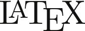 .
.
The remainder of this paper discusses key components of the SymPy library. Section ‘Overview of capabilities’ enumerates the features of SymPy and takes a closer look at some of the important ones. The Section ‘Numerics’ looks at the numerical features of SymPy and its dependency library, mpmath. Section ‘Physics Submodule’ looks at the domain specific physics submodules for performing symbolic and numerical calculations in classical mechanics and quantum mechanics. Section ‘Architecture’ discusses the architecture of SymPy. Section ‘Projects that Depend on SymPy’ looks at a selection of packages that depend on SymPy. Conclusions and future directions for SymPy are given in ‘Conclusion and Future Work’. All examples in this paper use SymPy version 1.0 and mpmath version 0.19.
Additionally, the Supplemental Information 1 takes a deeper look at a few SymPy topics. Section S1 discusses the Gruntz algorithm, which SymPy uses to calculate symbolic limits. Sections S2–S9 of the supplement discuss the series, logic, Diophantine equations, sets, statistics, category theory, tensor, and numerical simplification submodules of SymPy, respectively. Section S10 provides additional examples for topics discussed in the main paper. Section S11 discusses the SymPy Gamma project. Finally, Section S12 of the supplement contains a brief comparison of SymPy with Wolfram Mathematica.
The following statement imports all SymPy functions into the global Python namespace.2 From here on, all examples in this paper assume that this statement has been executed3:
>>> from sympy import *All the examples in this paper can be tested on SymPy Live, an online Python shell that uses the Google App Engine (Ciurana, 2009) to execute SymPy code. SymPy Live is also integrated into the SymPy documentation at http://docs.sympy.org.
Overview of capabilities
This section gives a basic introduction of SymPy, and lists its features. A few features—assumptions, simplification, calculus, polynomials, printers, solvers, and matrices—are core components of SymPy and are discussed in depth. Many other features are discussed in depth in the Supplemental Information 1.
Basic usage
Symbolic variables, called symbols, must be defined and assigned to Python variables before they can be used. This is typically done through the symbols function, which may create multiple symbols in a single function call. For instance,
>>> x, y, z = symbols('x y z')creates three symbols representing variables named x, y, and z. In this particular instance, these symbols are all assigned to Python variables of the same name. However, the user is free to assign them to different Python variables, while representing the same symbol, such as a, b, c = symbols('x y z'). In order to minimize potential confusion, though, all examples in this paper will assume that the symbols x , y , and z have been assigned to Python variables identical to their symbolic names.
Expressions are created from symbols using Python’s mathematical syntax. For instance, the following Python code creates the expression (x2 − 2x + 3)∕y. Note that the expression remains unevaluated: it is represented symbolically.
>>> (x**2 - 2*x + 3)/y
(x**2 - 2*x + 3)/y
List of features
Although SymPy’s extensive feature set cannot be covered in depth in this paper, bedrock areas, that is, those areas that are used throughout the library, are discussed in their own subsections below. Additionally, Table 1 gives a compact listing of all major capabilities present in the SymPy codebase. This grants a sampling from the breadth of topics and application domains that SymPy services. Unless stated otherwise, all features noted in Table 1 are symbolic in nature. Numeric features are discussed in Section ‘Numerics.’
| Feature (submodules) | Description |
|---|---|
| Calculus (sympy.core, sympy.calculus, sympy.integrals, sympy.series) | Algorithms for computing derivatives, integrals, and limits. |
| Category Theory (sympy.categories) | Representation of objects, morphisms, and diagrams. Tools for drawing diagrams with Xy-pic (Rose, 1999). |
| Code Generation (sympy.printing, sympy.codegen) | Generation of compilable and executable code in a variety of different programming languages from expressions directly. Target languages include C, Fortran, Julia, JavaScript, Mathematica, MATLAB and Octave, Python, and Theano. |
| Combinatorics & Group Theory (sympy.combinatorics) | Permutations, combinations, partitions, subsets, various permutation groups (such as polyhedral, Rubik, symmetric, and others), Gray codes (Nijenhuis & Wilf, 1978), and Prufer sequences (Biggs, Lloyd & Wilson, 1976). |
| Concrete Math (sympy.concrete) | Summation, products, tools for determining whether summation and product expressions are convergent, absolutely convergent, hypergeometric, and for determining other properties; computation of Gosper’s normal form (Petkovšek, Wilf & Zeilberger, 1997) for two univariate polynomials. |
| Cryptography (sympy.crypto) | Block and stream ciphers, including shift, Affine, substitution, Vigenère’s, Hill’s, bifid, RSA, Kid RSA, linear-feedback shift registers, and Elgamal encryption. |
| Differential Geometry (sympy.diffgeom) | Representations of manifolds, metrics, tensor products, and coordinate systems in Riemannian and pseudo-Riemannian geometries (Sussman & Wisdom, 2013). |
| Geometry (sympy.geometry) | Representations of 2D geometrical entities, such as lines and circles. Enables queries on these entities, such as asking the area of an ellipse, checking for collinearity of a set of points, or finding the intersection between objects. |
| Lie Algebras (sympy.liealgebras) | Representations of Lie algebras and root systems. |
| Logic (sympy.logic) | Boolean expressions, equivalence testing, satisfiability, and normal forms. |
| Matrices (sympy.matrices) | Tools for creating matrices of symbols and expressions. Both sparse and dense representations, as well as symbolic linear algebraic operations (e.g., inversion and factorization), are supported. |
| Matrix Expressions (sympy.matrices.expressions) | Matrices with symbolic dimensions (unspecified entries). Block matrices. |
| Number Theory (sympy.ntheory) | Prime number generation, primality testing, integer factorization, continued fractions, Egyptian fractions, modular arithmetic, quadratic residues, partitions, binomial and multinomial coefficients, prime number tools, hexidecimal digits of π, and integer factorization. |
| Plotting (sympy.plotting) | Hooks for visualizing expressions via matplotlib (Hunter, 2007) or as text drawings when lacking a graphical back-end. 2D function plotting, 3D function plotting, and 2D implicit function plotting are supported. |
| Polynomials (sympy.polys) | Polynomial algebras over various coefficient domains. Functionality ranges from simple operations (e.g., polynomial division) to advanced computations (e.g., Gröbner bases (Adams & Loustaunau, 1994) and multivariate factorization over algebraic number domains). |
| Printing (sympy.printing) | Functions for printing SymPy expressions in the terminal with ASCII or Unicode characters and converting SymPy expressions to and MathML. |
| Quantum Mechanics (sympy.physics.quantum) | Quantum states, bra–ket notation, operators, basis sets, representations, tensor products, inner products, outer products, commutators, anticommutators, and specific quantum system implementations. |
| Series (sympy.series) | Series expansion, sequences, and limits of sequences. This includes Taylor, Laurent, and Puiseux series as well as special series, such as Fourier and formal power series. |
| Sets (sympy.sets) | Representations of empty, finite, and infinite sets (including special sets such as the natural, integer, and complex numbers). Operations on sets such as union, intersection, Cartesian product, and building sets from other sets are supported. |
| Simplification (sympy.simplify) | Functions for manipulating and simplifying expressions. Includes algorithms for simplifying hypergeometric functions, trigonometric expressions, rational functions, combinatorial functions, square root denesting, and common subexpression elimination. |
| Solvers (sympy.solvers) | Functions for symbolically solving equations, systems of equations, both linear and non-linear, inequalities, ordinary differential equations, partial differential equations, Diophantine equations, and recurrence relations. |
| Special Functions (sympy.functions) | Implementations of a number of well known special functions, including Dirac delta, Gamma, Beta, Gauss error functions, Fresnel integrals, Exponential integrals, Logarithmic integrals, Trigonometric integrals, Bessel, Hankel, Airy, B-spline, Riemann Zeta, Dirichlet eta, polylogarithm, Lerch transcendent, hypergeometric, elliptic integrals, Mathieu, Jacobi polynomials, Gegenbauer polynomial, Chebyshev polynomial, Legendre polynomial, Hermite polynomial, Laguerre polynomial, and spherical harmonic functions. |
| Statistics (sympy.stats) | Support for a random variable type as well as the ability to declare this variable from prebuilt distribution functions such as Normal, Exponential, Coin, Die, and other custom distributions (Rocklin & Terrel, 2012). |
| Tensors (sympy.tensor) | Symbolic manipulation of indexed objects. |
| Vectors (sympy.vector) | Basic operations on vectors and differential calculus with respect to 3D Cartesian coordinate systems. |
Assumptions
The assumptions system allows users to specify that symbols have certain common mathematical properties, such as being positive, imaginary, or integer. SymPy is careful to never perform simplifications on an expression unless the assumptions allow them. For instance, the simplification holds if t is nonnegative (t ≥ 0), but it does not hold for a general complex t.4
By default, SymPy performs all calculations assuming that symbols are complex valued. This assumption makes it easier to treat mathematical problems in full generality.
>>> t = Symbol('t')
>>> sqrt(t**2)
sqrt(t**2)
By assuming the most general case, that t is complex by default, SymPy avoids performing mathematically invalid operations. However, in many cases users will wish to simplify expressions containing terms like .
Assumptions are set on Symbol objects when they are created. For instance Symbol('t', positive=True) will create a symbol named t that is assumed to be positive.
>>> t = Symbol('t', positive=True)
>>> sqrt(t**2)
t
Some of the common assumptions are negative, real, nonpositive, integer, prime and commutative.5 Assumptions on any SymPy object can be checked with the is_ assumption attributes, like t.is_positive .
Assumptions are only needed to restrict a domain so that certain simplifications can be performed. They are not required to make the domain match the input of a function. For instance, one can create the object as Sum(f(n), (n, 0, m)) without setting integer=True when creating the Symbol object n.
The assumptions system additionally has deductive capabilities. The assumptions use a three-valued logic using the Python built in objects True, False, and None. Note that False is returned if the SymPy object doesn’t or can’t have the assumption. For example, both I.is_real and I.is_prime return False for the imaginary unit I.
None represents the “unknown” case. This could mean that given assumptions do not unambiguously specify the truth of an attribute. For instance, Symbol('x', real=True).is_positive will give None because a real symbol might be positive or negative. None could also mean that not enough is known or implemented to compute the given fact. For instance, (pi + E).is_irrational gives None—indeed, the rationality of π + e is an open problem in mathematics (Lang, 1966).
Basic implications between the facts are used to deduce assumptions. Deductions are made using the Rete algorithm (Doorenbos, 1995).6 For instance, the assumptions system knows that being an integer implies being rational.
>>> i = Symbol('i', integer=True)
>>> i.is_rational
True
Furthermore, expressions compute the assumptions on themselves based on the assumptions of their arguments. For instance, if x and y are both created with positive=True, then (x + y).is_positive will be True (whereas (x - y).is_positive will be None).
Simplification
The generic way to simplify an expression is by calling the simplify function. It must be emphasized that simplification is not a rigorously defined mathematical operation (Moses, 1971). The simplify function applies several simplification routines along with heuristics to make the output expression “simple”.7
It is often preferable to apply more directed simplification functions. These apply very specific rules to the input expression and are typically able to make guarantees about the output. For instance, the factor function, given a polynomial with rational coefficients in several variables, is guaranteed to produce a factorization into irreducible factors. Table 2 lists common simplification functions.
| expand | expand the expression |
| factor | factor a polynomial into irreducibles |
| collect | collect polynomial coefficients |
| cancel | rewrite a rational function as p∕q with common factors canceled |
| apart | compute the partial fraction decomposition of a rational function |
| trigsimp | simplify trigonometric expressions (Fu, Zhong & Zeng, 2006) |
| hyperexpand | expand hypergeometric functions (Roach, 1996; Roach, 1997) |
Examples for these simplification functions can be found in Section S10.
Calculus
SymPy provides all the basic operations of calculus, such as calculating limits, derivatives, integrals, or summations.
Limits are computed with the limit function, using the Gruntz algorithm (Gruntz, 1996) for computing symbolic limits and heuristics (a description of the Gruntz algorithm may be found in Section S1). For example, the following computes . Note that SymPy denotes ∞ as oo (two lower case “o”s).
>>> limit(x*sin(1/x), x, oo)
1
As a more complex example, SymPy computes
>>> limit((2*exp((1-cos(x))/sin(x))-1)**(sinh(x)/atan(x)**2), x, 0)
E
Derivatives are computed with the diff function, which recursively uses the various differentiation rules.
>>> diff(sin(x)*exp(x), x)
exp(x)*sin(x) + exp(x)*cos(x)
Integrals are calculated with the integrate function. SymPy implements a combination of the Risch algorithm (Bronstein, 2005b), table lookups, a reimplementation of Manuel Bronstein’s “Poor Man’s Integrator” (Bronstein, 2005a), and an algorithm for computing integrals based on Meijer G-functions (Roach, 1996; Roach, 1997). These allow SymPy to compute a wide variety of indefinite and definite integrals. The Meijer G-function algorithm and the Risch algorithm are respectively demonstrated below by the computation of
and
>>> s, t = symbols('s t', positive=True)
>>> integrate(exp(-s*t)*log(t), (t, 0, oo)).simplify()
-(log(s) + EulerGamma)/s
>>> integrate((-2*x**2*(log(x) + 1)*exp(x**2) +
... (exp(x**2) + 1)**2)/(x*(exp(x**2) + 1)**2*(log(x) + 1)), x)
log(log(x) + 1) + 1/(exp(x**2) + 1)
Summations are computed with the summation function, which uses a combination of Gosper’s algorithm (Gosper, 1978), an algorithm that uses Meijer G-functions (Roach, 1996; Roach, 1997), and heuristics. Products are computed with product function via a suite of heuristics.
>>> i, n = symbols('i n')
>>> summation(2**i, (i, 0, n - 1))
2**n - 1
>>> summation(i*factorial(i), (i, 1, n))
n*factorial(n) + factorial(n) - 1
Series expansions are computed with the series function. This example computes the power series of sin(x) around x = 0 up to x6.
>>> series(sin(x), x, 0, 6)
x - x**3/6 + x**5/120 + O(x**6)
Section S2 discusses series expansions methods in more depth. Integrals, derivatives, summations, products, and limits that cannot be computed return unevaluated objects. These can also be created directly if the user chooses.
>>> integrate(x**x, x)
Integral(x**x, x)
>>> Sum(2**i, (i, 0, n - 1))
Sum(2**i, (i, 0, n - 1))
Polynomials
SymPy implements a suite of algorithms for polynomial manipulation, which ranges from relatively simple algorithms for doing arithmetic of polynomials, to advanced methods for factoring multivariate polynomials into irreducibles, symbolically determining real and complex root isolation intervals, or computing Gröbner bases.
Polynomial manipulation is useful in its own right. Within SymPy, though, it is mostly used indirectly as a tool in other areas of the library. In fact, many mathematical problems in symbolic computing are first expressed using entities from the symbolic core, preprocessed, and then transformed into a problem in the polynomial algebra, where generic and efficient algorithms are used to solve the problem. The solutions to the original problem are subsequently recovered from the results. This is a common scheme in symbolic integration or summation algorithms.
SymPy implements dense and sparse polynomial representations.8 Both are used in the univariate and multivariate cases. The dense representation is the default for univariate polynomials. For multivariate polynomials, the choice of representation is based on the application. The most common case for the sparse representation is algorithms for computing Gröbner bases (Buchberger, F4, and F5) (Buchberger, 1965; Faugère, 1999; Faugère, 2002). This is because different monomial orderings can be expressed easily in this representation. However, algorithms for computing multivariate GCDs or factorizations, at least those currently implemented in SymPy (Paprocki, 2010), are better expressed when the representation is dense. The dense multivariate representation is specifically a recursively-dense representation, where polynomials in K[x0, x1, …, xn] are viewed as a polynomials in K[x0][x1]…[xn]. Note that despite this, the coefficient domain K, can be a multivariate polynomial domain as well. The dense recursive representation in Python gets inefficient as the number of variables increases.
Some examples for the sympy.polys submodule can be found in Section S10.
Printers
SymPy has a rich collection of expression printers. By default, an interactive Python session will render the str form of an expression, which has been used in all the examples in this paper so far. The str form of an expression is valid Python and roughly matches what a user would type to enter the expression.9
>>> phi0 = Symbol('phi0')
>>> str(Integral(sqrt(phi0), phi0))
'Integral(sqrt(phi0), phi0)'
A two-dimensional (2D) textual representation of the expression can be printed with monospace fonts via pprint. Unicode characters are used for rendering mathematical symbols such as integral signs, square roots, and parentheses. Greek letters and subscripts in symbol names that have Unicode code points associated are also rendered automatically.
Alternately, the use_unicode=False flag can be set, which causes the expression to be printed using only ASCII characters.
>>> pprint(Integral(sqrt(phi0 + 1), phi0), use_unicode=False)
  /
 |
 |   __________
 | \/ phi0 + 1  d(phi0)
 |
/
The function latex returns a representation of an expression.
>>> print(latex(Integral(sqrt(phi0 + 1), phi0)))
\int \sqrt{\phi_{0} + 1}\, d\phi_{0}
Users are encouraged to run the init_printing function at the beginning of interactive sessions, which automatically enables the best pretty printing supported by their environment. In the Jupyter Notebook or Qt Console (Pérez & Granger, 2007), the printer is used to render expressions using MathJax or , if it is installed on the system. The 2D text representation is used otherwise.
Other printers such as MathML are also available. SymPy uses an extensible printer subsystem, which allows extending any given printer, and also allows custom objects to define their printing behavior for any printer. The code generation functionality of SymPy relies on this subsystem to convert expressions into code in various target programming languages.
Solvers
SymPy has equation solvers that can handle ordinary differential equations, recurrence relationships, Diophantine equations,10 and algebraic equations. There is also rudimentary support for simple partial differential equations.
There are two functions for solving algebraic equations in SymPy: solve and solveset. solveset has several design changes with respect to the older solve function. This distinction is present in order to resolve the usability issues with the previous solve function API while maintaining backward compatibility with earlier versions of SymPy. solveset only requires essential input information from the user. The function signatures of solve and solveset are
solve(f, *symbols, **flags)
solveset(f, symbol, domain=S.Complexes)
The domain parameter can be any set from the sympy.sets module (see Section S5 for details on sympy.sets), but is typically either S.Complexes (the default) or S.Reals; the latter causes solveset to only return real solutions.
An important difference between the two functions is that the output API of solve varies with input (sometimes returning a Python list and sometimes a Python dictionary) whereas solveset always returns a SymPy set object.
Both functions implicitly assume that expressions are equal to 0. For instance, solveset(x - 1, x) solves x − 1 = 0 for x.
solveset is under active development as a planned replacement for solve. There are certain features which are implemented in solve that are not yet implemented in solveset, including multivariate systems, and some transcendental equations.
Some examples for solveset and solve can be found in Section S10.
Matrices
Besides being an important feature in its own right, computations on matrices with symbolic entries are important for many algorithms within SymPy. The following code shows some basic usage of the Matrix class.
>>> A = Matrix([[x, x + y], [y, x]])
>>> A
Matrix([
[x, x + y],
[y,     x]])
SymPy matrices support common symbolic linear algebra manipulations, including matrix addition, multiplication, exponentiation, computing determinants, solving linear systems, singular values, and computing inverses using LU decomposition, LDL decomposition, Gauss-Jordan elimination, Cholesky decomposition, Moore–Penrose pseudoinverse, or adjugate matrices.
All operations are performed symbolically. For instance, eigenvalues are computed by generating the characteristic polynomial using the Berkowitz algorithm and then finding its zeros using polynomial routines.
>>> A.eigenvals()
{x - sqrt(y*(x + y)): 1, x + sqrt(y*(x + y)): 1}
Internally these matrices store the elements as Lists of Lists (LIL) (Jones et al., 2001), meaning the matrix is stored as a list of lists of entries (effectively, the input format used to create the matrix A above), making it a dense representation.11 For storing sparse matrices, the SparseMatrix class can be used. Sparse matrices store their elements in Dictionary of Keys (DOK) format, meaning that the entries are stored as a dict of (row, column) pairs mapping to the elements.
SymPy also supports matrices with symbolic dimension values. MatrixSymbol represents a matrix with dimensions m × n, where m and n can be symbolic. Matrix addition and multiplication, scalar operations, matrix inverse, and transpose are stored symbolically as matrix expressions.
Block matrices are also implemented in SymPy. BlockMatrix elements can be any matrix expression, including explicit matrices, matrix symbols, and other block matrices. All functionalities of matrix expressions are also present in BlockMatrix .
When symbolic matrices are combined with the assumptions submodule for logical inference, they provide powerful reasoning over invertibility, semi-definiteness, orthogonality, etc., which are valuable in the construction of numerical linear algebra systems (Rocklin, 2013).
More examples for Matrix and BlockMatrix may be found in Section S10.
Numerics
While SymPy primarily focuses on symbolics, it is impossible to have a complete symbolic system without the ability to numerically evaluate expressions. Many operations directly use numerical evaluation, such as plotting a function, or solving an equation numerically. Beyond this, certain purely symbolic operations require numerical evaluation to effectively compute. For instance, determining the truth value of e + 1 > π is most conveniently done by numerically evaluating both sides of the inequality and checking which is larger.
Floating-point numbers
Floating-point numbers in SymPy are implemented by the Float class, which represents an arbitrary-precision binary floating-point number by storing its value and precision (in bits). This representation is distinct from the Python built-in float type, which is a wrapper around machine double types and uses a fixed precision (53-bit).
Because Python float literals are limited in precision, strings should be used to input precise decimal values:
>>> Float(1.1)
1.10000000000000
>>> Float(1.1, 30)   # precision equivalent to 30 digits
1.10000000000000008881784197001
>>> Float("1.1", 30)
1.10000000000000000000000000000
The evalf method converts a constant symbolic expression to a Float with the specified precision, here 25 digits:
>>> (pi + 1).evalf(25)
4.141592653589793238462643
Float numbers do not track their accuracy, and should be used with caution within symbolic expressions since familiar dangers of floating-point arithmetic apply (Goldberg, 1991). A notorious case is that of catastrophic cancellation:
>>> cos(exp(-100)).evalf(25) - 1
0
Applying the evalf method to the whole expression solves this problem. Internally, evalf estimates the number of accurate bits of the floating-point approximation for each sub-expression, and adaptively increases the working precision until the estimated accuracy of the final result matches the sought number of decimal digits:
>>> (cos(exp(-100)) - 1).evalf(25)
-6.919482633683687653243407e-88
The evalf method works with complex numbers and supports more complicated expressions, such as special functions, infinite series, and integrals. The internal error tracking does not provide rigorous error bounds (in the sense of interval arithmetic) and cannot be used to accurately track uncertainty in measurement data; the sole purpose is to mitigate loss of accuracy that typically occurs when converting symbolic expressions to numerical values.
The mpmath library
The implementation of arbitrary-precision floating-point arithmetic is supplied by the mpmath library (Johansson & The mpmath Development Team, 2014). Originally, it was developed as a SymPy submodule but has subsequently been moved to a standalone pure-Python package. The basic datatypes in mpmath are mpf and mpc, which respectively act as multiprecision substitutes for Python’s float and complex. The floating-point precision is controlled by a global context:
>>> import mpmath
>>> mpmath.mp.dps = 30    # 30 digits of precision
>>> mpmath.mpf("0.1") + mpmath.exp(-50)
mpf('0.100000000000000000000192874984794')
>>> print(_)   # pretty-printed
0.100000000000000000000192874985
Like SymPy, mpmath is a pure Python library. A design decision of SymPy is to keep it and its required dependencies pure Python. This is a primary advantage of mpmath over other multiple precision libraries such as GNU MPFR (Fousse et al., 2007), which is faster. Like SymPy, mpmath is also BSD licensed (GNU MPFR is licensed under the GNU Lesser General Public License (Rosen, 2005)).
Internally, mpmath represents a floating-point number (−1)sx⋅2y by a tuple (s, x, y, b) where x and y are arbitrary-size Python integers and the redundant integer b stores the bit length of x for quick access. If GMPY (Horsen, 2015) is installed, mpmath automatically uses the gmpy.mpz type for x, and GMPY methods for rounding-related operations, improving performance.
Most mpmath and SymPy functions use the same naming scheme, although this is not true in every case. For example, the symbolic SymPy summation expression Sum(f(x), (x, a, b)) representing is represented in mpmath as nsum(f, (a, b)), where f is a numeric Python function.
The mpmath library supports special functions, root-finding, linear algebra, polynomial approximation, and numerical computation of limits, derivatives, integrals, infinite series, and solving ODEs. All features work in arbitrary precision and use algorithms that allow computing hundreds of digits rapidly (except in degenerate cases).
The double exponential (tanh-sinh) quadrature is used for numerical integration by default. For smooth integrands, this algorithm usually converges extremely rapidly, even when the integration interval is infinite or singularities are present at the endpoints (Takahasi & Mori, 1974; Bailey, Jeyabalan & Li, 2005). However, for good performance, singularities in the middle of the interval must be specified by the user. To evaluate slowly converging limits and infinite series, mpmath automatically tries Richardson extrapolation and the Shanks transformation (Euler-Maclaurin summation can also be used) (Bender & Orszag, 1999). A function to evaluate oscillatory integrals by means of convergence acceleration is also available.
A wide array of higher mathematical functions is implemented with full support for complex values of all parameters and arguments, including complete and incomplete gamma functions, Bessel functions, orthogonal polynomials, elliptic functions and integrals, zeta and polylogarithm functions, the generalized hypergeometric function, and the Meijer G-function. The Meijer G-function instance is a good test case (Toth, 2007); past versions of both Maple and Mathematica produced incorrect numerical values for large x > 0. Here, mpmath automatically removes an internal singularity and compensates for cancellations (amounting to 656 bits of precision when x = 10, 000), giving correct values:
>>> mpmath.mp.dps = 15
>>> mpmath.meijerg([[],[0]], [[-0.5,-1,-1.5],[]], 10000)
mpf('2.4392576907199564e-94')
Equivalently, with SymPy’s interface this function can be evaluated as:
>>> meijerg([[],[0]], [[-S(1)/2,-1,-S(3)/2],[]], 10000).evalf()
2.43925769071996e-94
Symbolic integration and summation often produce hypergeometric and Meijer G-function closed forms (see Section ‘Calculus’); numerical evaluation of such special functions is a useful complement to direct numerical integration and summation.
Physics submodule
SymPy includes several submodules that allow users to solve domain specific physics problems. For example, a comprehensive physics submodule is included that is useful for solving problems in mechanics, optics, and quantum mechanics along with support for manipulating physical quantities with units.
Classical mechanics
One of the core domains that SymPy suports is the physics of classical mechanics. This is in turn separated into two distinct components: vector algebra and mechanics.
Vector algebra
The sympy.physics.vector submodule provides reference frame-, time-, and space-aware vector and dyadic objects that allow for three-dimensional operations such as addition, subtraction, scalar multiplication, inner and outer products, and cross products. The vector and dyadic objects both can be written in very compact notation that make it easy to express the vectors and dyadics in terms of multiple reference frames with arbitrarily defined relative orientations. The vectors are used to specify the positions, velocities, and accelerations of points; orientations, angular velocities, and angular accelerations of reference frames; and forces and torques. The dyadics are essentially reference frame-aware 3 × 3 tensors (Tai, 1997). The vector and dyadic objects can be used for any one-, two-, or three-dimensional vector algebra, and they provide a strong framework for building physics and engineering tools.
The following Python code demonstrates how a vector is created using the orthogonal unit vectors of three reference frames that are oriented with respect to each other, and the result of expressing the vector in the A frame. The B frame is oriented with respect to the A frame using Z-X-Z Euler Angles of magnitude π, , and , respectively, whereas the C frame is oriented with respect to the B frame through a simple rotation about the B frame’s X unit vector through .
>>> from sympy.physics.vector import ReferenceFrame
>>> A, B, C = symbols('A B C', cls=ReferenceFrame)
>>> B.orient(A, 'body', (pi, pi/3, pi/4), 'zxz')
>>> C.orient(B, 'axis', (pi/2, B.x))
>>> v = 1*A.x + 2*B.z + 3*C.y
>>> v
A.x + 2*B.z + 3*C.y
>>> v.express(A)
A.x + 5*sqrt(3)/2*A.y + 5/2*A.z
Mechanics
The sympy.physics.mechanics submodule utilizes the sympy.physics.vector submodule to populate time-aware particle and rigid-body objects to fully describe the kinematics and kinetics of a rigid multi-body system. These objects store all of the information needed to derive the ordinary differential or differential algebraic equations that govern the motion of the system, i.e., the equations of motion. These equations of motion abide by Newton’s laws of motion and can handle arbitrary kinematic constraints or complex loads. The submodule offers two automated methods for formulating the equations of motion based on Lagrangian Dynamics (Lagrange, 1811) and Kane’s Method (Kane & Levinson, 1985). Lastly, there are automated linearization routines for constrained dynamical systems (Peterson, Gede & Hubbard, 2014).
Quantum mechanics
The sympy.physics.quantum submodule has extensive capabilities to solve problems in quantum mechanics, using Python objects to represent the different mathematical objects relevant in quantum theory (Sakurai & Napolitano, 2010): states (bras and kets), operators (unitary, Hermitian, etc.), and basis sets, as well as operations on these objects such as representations, tensor products, inner products, outer products, commutators, and anticommutators. The base objects are designed in the most general way possible to enable any particular quantum system to be implemented by subclassing the base operators and defining the relevant class methods to provide system-specific logic.
Symbolic quantum operators and states may be defined, and one can perform a full range of operations with them.
>>> from sympy.physics.quantum import Commutator, Dagger, Operator
>>> from sympy.physics.quantum import Ket, qapply
>>> A, B, C, D = symbols('A B C D', cls=Operator)
>>> a = Ket('a')
>>> comm = Commutator(A, B)
>>> comm
[A,B]
>>> qapply(Dagger(comm*a)).doit()
-<a|*(Dagger(A)*Dagger(B) - Dagger(B)*Dagger(A))
Commutators can be expanded using common commutator identities:
>>> Commutator(C+B, A*D).expand(commutator=True)
-[A,B]*D - [A,C]*D + A*[B,D] + A*[C,D]
On top of this set of base objects, a number of specific quantum systems have been implemented in a fully symbolic framework. These include:
-
Many of the exactly solvable quantum systems, including simple harmonic oscillator states and raising/lowering operators, infinite square well states, and 3D position and momentum operators and states.
-
Second quantized formalism of non-relativistic many-body quantum mechanics (Fetter & Walecka, 2003).
-
Quantum angular momentum (Zare, 1991). Spin operators and their eigenstates can be represented in any basis and for any quantum numbers. A rotation operator representing the Wigner D-matrix, which may be defined symbolically or numerically, is also implemented to rotate spin eigenstates. Functionality for coupling and uncoupling of arbitrary spin eigenstates is provided, including symbolic representations of Clebsch-Gordon coefficients and Wigner symbols.
-
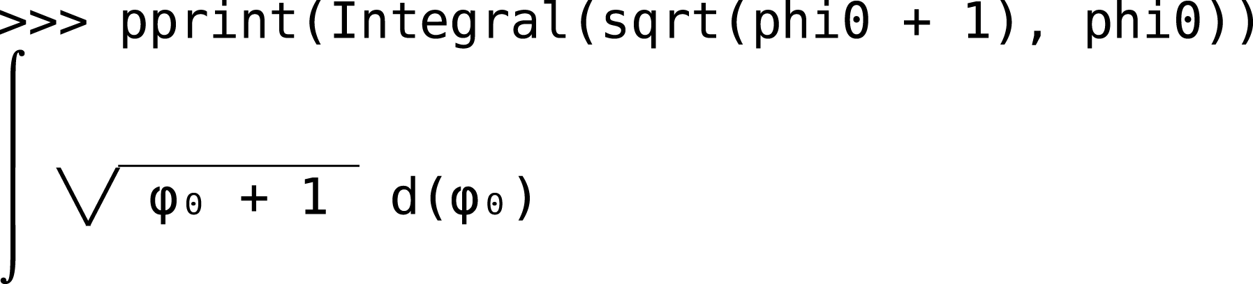
Quantum information and computing (Nielsen & Chuang, 2011). Multidimensional qubit states, and a full set of one- and two-qubit gates are provided and can be represented symbolically or as matrices/vectors. With these building blocks, it is possible to implement a number of basic quantum algorithms including the quantum Fourier transform, quantum error correction, quantum teleportation, Grover’s algorithm, dense coding, etc. In addition, any quantum circuit may be plotted using the circuit_plot function (Fig. 1).
Here are a few short examples of the quantum information and computing capabilities in sympy.physics.quantum . Start with a simple four-qubit state and flip the second qubit from the right using a Pauli-X gate:
>>> from sympy.physics.quantum.qubit import Qubit
>>> from sympy.physics.quantum.gate import XGate
>>> q = Qubit('0101')
>>> q
|0101>
>>> X = XGate(1)
>>> qapply(X*q)
|0111>
Qubit states can also be used in adjoint operations, tensor products, inner/outer products:
>>> Dagger(q)
<0101|
>>> ip = Dagger(q)*q
>>> ip
<0101|0101>
>>> ip.doit()
1
Quantum gates (unitary operators) can be applied to transform these states and then classical measurements can be performed on the results:
>>> from sympy.physics.quantum.qubit import measure_all
>>> from sympy.physics.quantum.gate import H, X, Y, Z
>>> c = H(0)*H(1)*Qubit('00')
>>> c
H(0)*H(1)*|00>
>>> q = qapply(c)
>>> measure_all(q)
[(|00>, 1/4), (|01>, 1/4), (|10>, 1/4), (|11>, 1/4)]
Lastly, the following example demonstrates creating a three-qubit quantum Fourier transform, decomposing it into one- and two-qubit gates, and then generating a circuit plot for the sequence of gates (see Fig. 1).
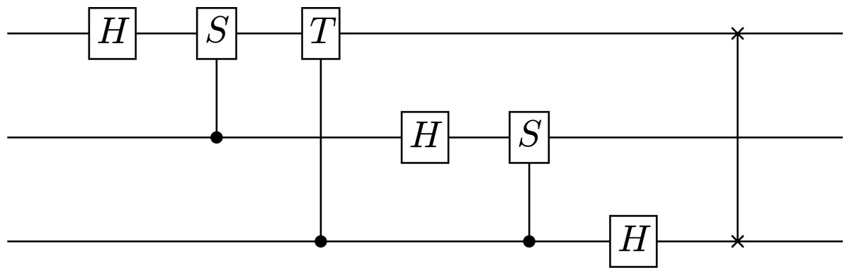
Figure 1: The circuit diagram for a three-qubit quantum Fourier transform generated by SymPy.
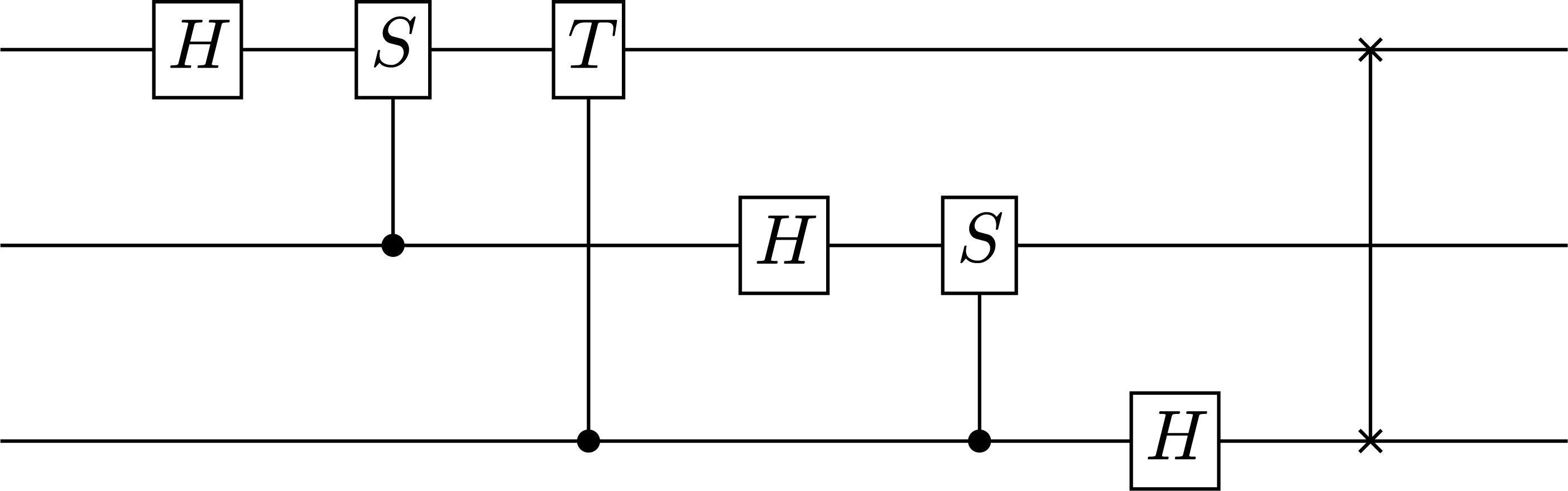
>>> from sympy.physics.quantum.qft import QFT
>>> from sympy.physics.quantum.circuitplot import circuit_plot
>>> fourier = QFT(0,3).decompose()
>>> fourier
SWAP(0,2)*H(0)*C((0),S(1))*H(1)*C((0),T(2))*C((1),S(2))*H(2)
>>> c = circuit_plot(fourier, nqubits=3)
Architecture
Software architecture is of central importance in any large software project because it establishes predictable patterns of usage and development (Shaw & Garlan, 1996). This section describes the essential structural components of SymPy, provides justifications for the design decisions that have been made, and gives example user-facing code as appropriate.
The core
A computer algebra system stores mathematical expressions as data structures. For example, the mathematical expression x + y is represented as a tree with three nodes, +, x, and y, where x and y are ordered children of +. As users manipulate mathematical expressions with traditional mathematical syntax, the CAS manipulates the underlying data structures. Symbolic computations such as integration, simplification, etc. are all functions that consume and produce expression trees.
In SymPy every symbolic expression is an instance of the class Basic,12 the superclass of all SymPy types providing common methods to all SymPy tree-elements, such as traversals. The children of a node in the tree are held in the args attribute. A leaf node in the expression tree has empty args.
For example, consider the expression xy + 2:
>>> x, y = symbols('x y')
>>> expr = x*y + 2
By order of operations, the parent of the expression tree for expr is an addition. It is of type Add. The child nodes of expr are 2 and x*y.
>>> type(expr)
<class 'sympy.core.add.Add'>
>>> expr.args
(2, x*y)
Descending further down into the expression tree yields the full expression. For example, the next child node (given by expr.args[0]) is 2. Its class is Integer, and it has an empty args tuple, indicating that it is a leaf node.
>>> expr.args[0]
2
>>> type(expr.args[0])
<class 'sympy.core.numbers.Integer'>
>>> expr.args[0].args
()
Symbols or symbolic constants, like e or π, are other examples of leaf nodes.
>>> exp(1)
E
>>> exp(1).args
()
>>> x.args
()
A useful way to view an expression tree is using the srepr function, which returns a string representation of an expression as valid Python code13 with all the nested class constructor calls to create the given expression.
>>> srepr(expr)
"Add(Mul(Symbol('x'), Symbol('y')), Integer(2))"
Every SymPy expression satisfies a key identity invariant:
expr.func(*expr.args) == exprThis means that expressions are rebuildable from their args.14 Note that in SymPy the == operator represents exact structural equality, not mathematical equality. This allows testing if any two expressions are equal to one another as expression trees. For example, even though (x + 1)2 and x2 + 2x + 1 are equal mathematically, SymPy gives
>>> (x + 1)**2 == x**2 + 2*x + 1
False
because they are different as expression trees (the former is a Pow object and the latter is an Add object).
Another important property of SymPy expressions is that they are immutable. This simplifies the design of SymPy, and enables expression interning. It also enables expressions to be hashed, which allows expressions to be used as keys in Python dictionaries, and is used to implement caching in SymPy.
Python allows classes to override mathematical operators. The Python interpreter translates the above x*y + 2 to, roughly, (x.__mul__(y)).__add__(2) . Both x and y, returned from the symbols function, are Symbol instances. The 2 in the expression is processed by Python as a literal, and is stored as Python’s built in int type. When 2 is passed to the __add__ method of Symbol, it is converted to the SymPy type Integer(2) before being stored in the resulting expression tree. In this way, SymPy expressions can be built in the natural way using Python operators and numeric literals.
Extensibility
While the core of SymPy is relatively small, it has been extended to a wide variety of domains by a broad range of contributors. This is due, in part, to the fact that the same language, Python, is used both for the internal implementation and the external usage by users. All of the extensibility capabilities available to users are also utilized by SymPy itself. This eases the transition pathway from SymPy user to SymPy developer.
The typical way to create a custom SymPy object is to subclass an existing SymPy class, usually Basic, Expr, or Function. As it was stated before, all SymPy classes used for expression trees should be subclasses of the base class Basic. Expr is the Basic subclass for mathematical objects that can be added and multiplied together. The most commonly seen classes in SymPy are subclasses of Expr, including Add, Mul, and Symbol. Instances of Expr typically represent complex numbers, but may also include other “rings”, like matrix expressions. Not all SymPy classes are subclasses of Expr. For instance, logic expressions, such as And(x, y) , are subclasses of Basic but not of Expr.15
The Function class is a subclass of Expr which makes it easier to define mathematical functions called with arguments. This includes named functions like sin(x) and log(x) as well as undefined functions like f(x). Subclasses of Function should define a class method eval, which returns an evaluated value for the function application (usually an instance of some other class, e.g., a Number), or None if for the given arguments it should not be automatically evaluated.
Many SymPy functions perform various evaluations down the expression tree. Classes define their behavior in such functions by defining a relevant _eval_ * method. For instance, an object can indicate to the diff function how to take the derivative of itself by defining the _eval_derivative(self, x) method, which may in turn call diff on its args. (Subclasses of Function should implement the fdiff method instead; it returns the derivative of the function without considering the chain rule.) The most common _eval_ * methods relate to the assumptions: _eval_is_ assumption is used to deduce assumption on the object.
Listing 1 presents an example of this extensibility. It gives a stripped down version of the gamma function Γ(x) from SymPy. The methods defined allow it to evaluate itself on positive integer arguments, define the real assumption, allow it to be rewritten in terms of factorial (with gamma(x).rewrite(factorial) ), and allow it to be differentiated. self.func is used throughout instead of referencing gamma explicitly so that potential subclasses of gamma can reuse the methods.
Listing 1: A minimal implementation of sympy.gamma.
from  sympy  import  Function, Integer, factorial, polygamma
class  gamma(Function):
     @classmethod
     def  eval(cls, arg):
          if  isinstance(arg, Integer) and  arg.is_positive:
               return  factorial(arg - 1)
     def  _eval_is_real(self):
          x = self.args[0]
          # noninteger  means  real  and  not  integer
          if x.is_positive  or x.is_noninteger:
               return  True
     def  _eval_rewrite_as_factorial(self, z):
          return  factorial(z - 1)
     def  fdiff(self, argindex=1):
          from  sympy.core.function  import  ArgumentIndexError
          if  argindex  == 1:
               return  self.func(self.args[0])*polygamma(0, self.args[0])
          else:
               raise  ArgumentIndexError(self, argindex)
The gamma function implemented in SymPy has many more capabilities than the above listing, such as evaluation at rational points and series expansion.
Performance
Due to being written in pure Python without the use of extension modules, SymPy’s performance characteristics are generally poorer than that of its commercial competitors. For many applications, the performance of SymPy, as measured by clock cycles, memory usage, and memory layout, is sufficient. However, the boundaries for when SymPy’s pure Python strategy becomes insufficient are when the user requires handling of very long expressions or many small expressions. Where this boundray lies depends on the system at hand, but tends to be within the range of 104–106 symbols for modern computers.
For this reason, a new project called SymEngine (The SymPy Developers, 2016a) has been started. The aim of this poject is to develop a library with better performance characteristics for symbolic manipulation. SymEngine is a pure C++ library, which allows it fine-grained control over the memory layout of expressions. SymEngine has thin wrappers to other languages (Python, Ruby, Julia, etc.). Its aim is to be the fastest symbolic manipulation library. Preliminary benchmarks suggest that SymEngine performs as well as its commercial and open source competitors.
The development version of SymPy has recently started to use SymEngine as an optional backend, initially in sympy.physics.mechanics only. Future work will involve allowing more algorithms in SymPy to use SymEngine as a backend.
Projects that depend on SymPy
There are several projects that depend on SymPy as a library for implementing a part of their functionality. A selection of these projects are listed in Table 3.
| Project name | Description |
|---|---|
| SymPy Gamma | An open source analog of Wolfram | Alpha that uses SymPy (The SymPy Developers, 2016b). There is more information about SymPy Gamma in Section S11. |
| Cadabra | A CAS designed specifically for the resolution of problems encountered in field theory (Peeters, 2007). |
| GNU Octave Symbolic Package | An implementation of a symbolic toolbox for Octave using SymPy (The Symbolic Package Developers, 2016). |
| SymPy.jl | A Julia interface to SymPy, provided using PyCall (The SymPy.jl Developers, 2016). |
| Mathics | A free, online CAS featuring Mathematica compatible syntax and functions (The Mathics Developers, 2016). |
| Mathpix | An iOS App that detects handwritten math as input and uses SymPy Gamma to evaluate the math input and generate the relevant steps to solve the problem (Mathpix, Inc., 2016). |
| IKFast | A robot kinematics compiler provided by OpenRAVE (Diankov, 2010). |
| SageMath | A free open-source mathematics software system, which builds on top of many existing open-source packages, including SymPy (The Sage Developers, 2016). |
| PyDy | Multibody Dynamics with Python (Gede et al., 2013). |
| galgebra | A Python package for geometric algebra (previously sympy.galgebra) (Bromborsky, 2016). |
| yt | A Python package for analyzing and visualizing volumetric data (Turk et al., 2011). |
| SfePy | A Python package for solving partial differential equations (PDEs) in 1D, 2D, and 3D by the finite element (FE) method (Zienkiewicz, Taylor & Zhu, 2013; Cimrman, 2014). |
| Quameon | Quantum Monte Carlo in Python (The Quameon Developers, 2016). |
| Lcapy | An experimental Python package for teaching linear circuit analysis (The Lcapy Developers, 2016). |
Conclusion and future work
SymPy is a robust computer algebra system that provides a wide spectrum of features both in traditional computer algebra and in a plethora of scientific disciplines. It can be used in a first-class way with other Python projects, including the scientific Python stack.
SymPy supports a wide array of mathematical facilities. These include functions for assuming and deducing common mathematical facts, simplifying expressions, performing common calculus operations, manipulating polynomials, pretty printing expressions, solving equations, and representing symbolic matrices. Other supported facilities include discrete math, concrete math, plotting, geometry, statistics, sets, series, vectors, combinatorics, group theory, code generation, tensors, Lie algebras, cryptography, and special functions. SymPy has strong support for arbitrary precision numerics, backed by the mpmath package. Additionally, SymPy contains submodules targeting certain specific physics domains, such as classical mechanics and quantum mechanics. This breadth of domains has been engendered by a strong and vibrant user community. Anecdotally, many of these users chose SymPy because of its ease of access. SymPy is a dependency of many external projects across a wide spectrum of domains.
SymPy expressions are immutable trees of Python objects. Unlike many other CAS’s, SymPy is designed to be used in an extensible way: both as an end-user application and as a library. SymPy uses Python both as the internal language and the user language. This permits users to access the same methods used by the library itself in order to extend it for their needs.
Some of the planned future work for SymPy includes work on improving code generation, improvements to the speed of SymPy using SymEngine, improving the assumptions system, and improving the solvers submodule.