2.1 UAV surveys

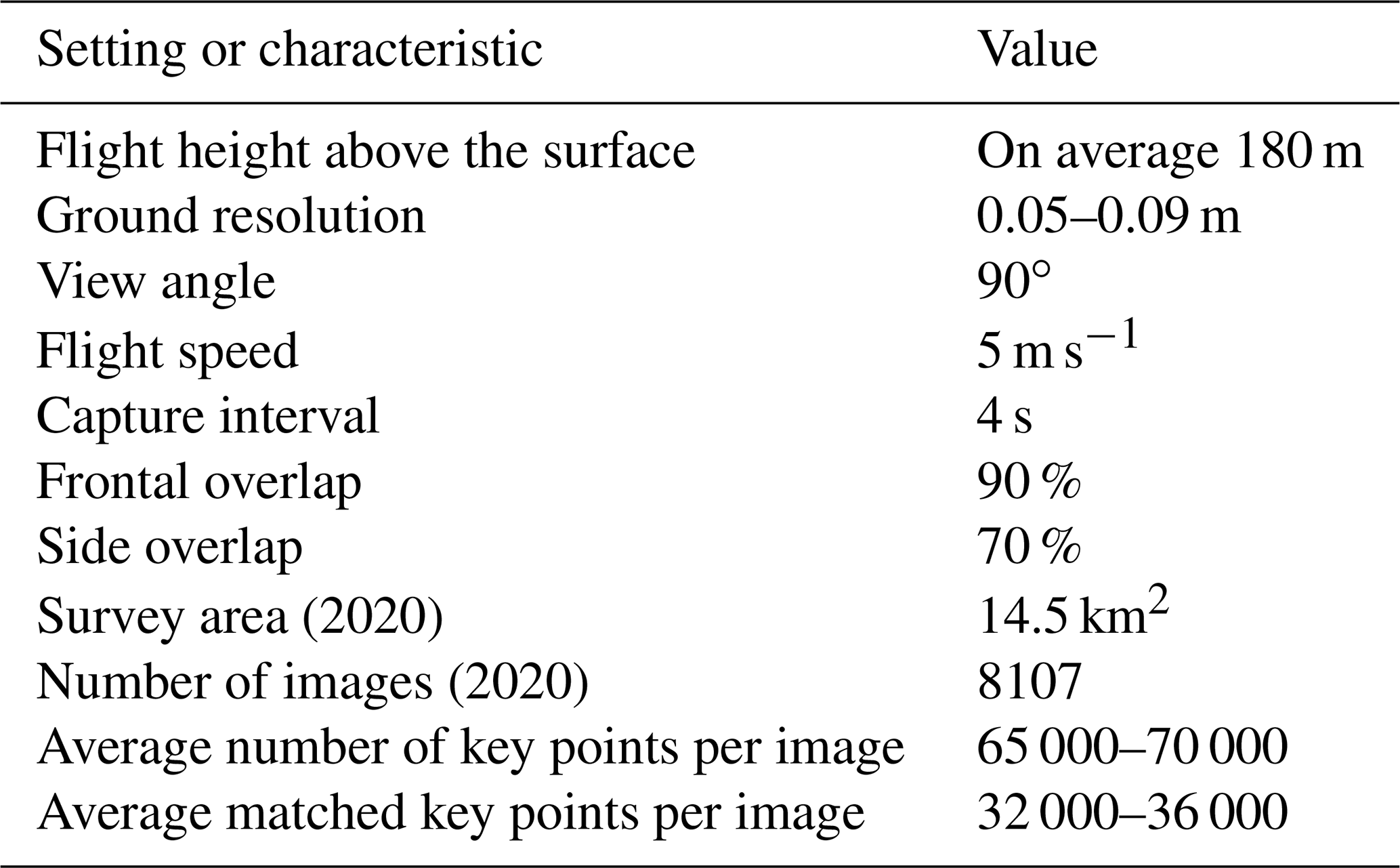
Between 2017 and 2020, we conducted annual UAV surveys at the end of the ablation season (late September). Hence, the focus in this research is on 3 mass balance years (2017–2018, 2018–2019 and 2019–2020). In 2017, above-normal snow cover and severe weather conditions prevented drone mapping on the upper parts of the ablation area of Vadret Pers (>2800 m) due to inadequate visual content for accurate key point detection (Gindraux et al., 2017) and the inability to distribute control points. This resulted in a smaller study area in 2017–2018. The observations consist of images acquired by repeated UAV surveys with a DJI Phantom 4 Pro (P4PRO) (in 2017, 2018 and 2019) and a DJI Phantom 4 RTK (P4RTK) (in 2020) quadcopter, both equipped with a 20-megapixel camera. For flight planning and UAV piloting, DJI GS Pro was used. The flight plans were designed to limit the variation in ground sampling distance (GSD) by flying parallel to the main surface slope and by subdividing the study area into smaller sections. We ensured in every case sufficient overlap between the different flight plans so that they could be easily attached to each other afterwards. Additional technical details of the flights are given in Table 1. The different flights within one field campaign were performed on multiple days. However, because of the short fieldwork periods (4–6 d), the difference between the SMB measurements and surface elevation changes caused by not surveying simultaneously is estimated to be at most up to 10 cm, which is within the uncertainty bounds of the measurements. Therefore, no correction was applied for the difference in acquisition dates.

Table 1Technical details and characteristics of the UAV flights.

Download Print Version | Download XLSX

To ensure sufficient horizontal and vertical accuracy, ground control points (GCPs) were distributed over the area of interest (see Fig. 2). The GCPs, plastic orange squares of 40×40 cm, were measured with a Trimble 7 GeoXH RTK GPS (horizontal average accuracy of 10–20 cm, vertical average accuracy of 20–30 cm) by relying on the Swiss Positioning Service (swipos) GIS/GEO. The GCPs were spread over different locations on the glacier following density and distribution guidelines from the literature (Tahar et al., 2012; Goldstein et al., 2015; Long et al., 2016; Tonkin and Midgley, 2016; Gindraux et al., 2017). We ensured homogeneous distribution in almost every case, except where crevasses, moulins or a fresh layer of snow (especially in 2017) impeded this, with an average density of 10–20 GCPs km⁻². Specific attention was paid to the distribution of GCPs in the overlapping areas of the different flight areas in order to be able to georeference two neighbouring flight areas with the same points. In 2020, a smaller number of GCPs were placed because the P4RTK can achieve centimetre-level accuracy without a large number of GCPs as a result of an on-board differential GPS system (Zhang et al., 2019; Kienholz et al., 2020). Each year, some of the GCPs were not used for the georeferencing process but as a ground validation point (GVP) to assess the quality of the reconstructed digital surface model (DSM).

2.2 In situ surface mass balance data

A total of 287 annual mass balance stake measurements (158 on Morteratsch, 129 on Pers) were performed between 2001 and 2020 in the ablation area of the glacier complex, with an average number of 15 stakes in each year. All the stakes were located between 2100 and 2600 m a.s.l. on the Morteratsch glacier's ablation tongue and between 2450 and 3050 m a.s.l. (approximately the equilibrium line altitude, ELA) on Vadret Pers. Zekollari and Huybrechts (2018) summarised these measurements and found the SMB rate on Pers glacier to be significantly lower (−2.1 to −2.5 m of ice equivalent (m i.e.) yr⁻¹) compared to Vadret da Morteratsch at similar elevation. This has been mainly attributed to differences in orientation and the associated daily insolation cycle over the two glaciers. For the period of concern in this study (2017–2020), SMB measurements from 16 individual stakes (8 on each glacier) are available for every year on the debris-free part of the ablation areas (Fig. 2). The stakes were measured and replaced if necessary annually at the end of each ablation season, during the UAV surveys.

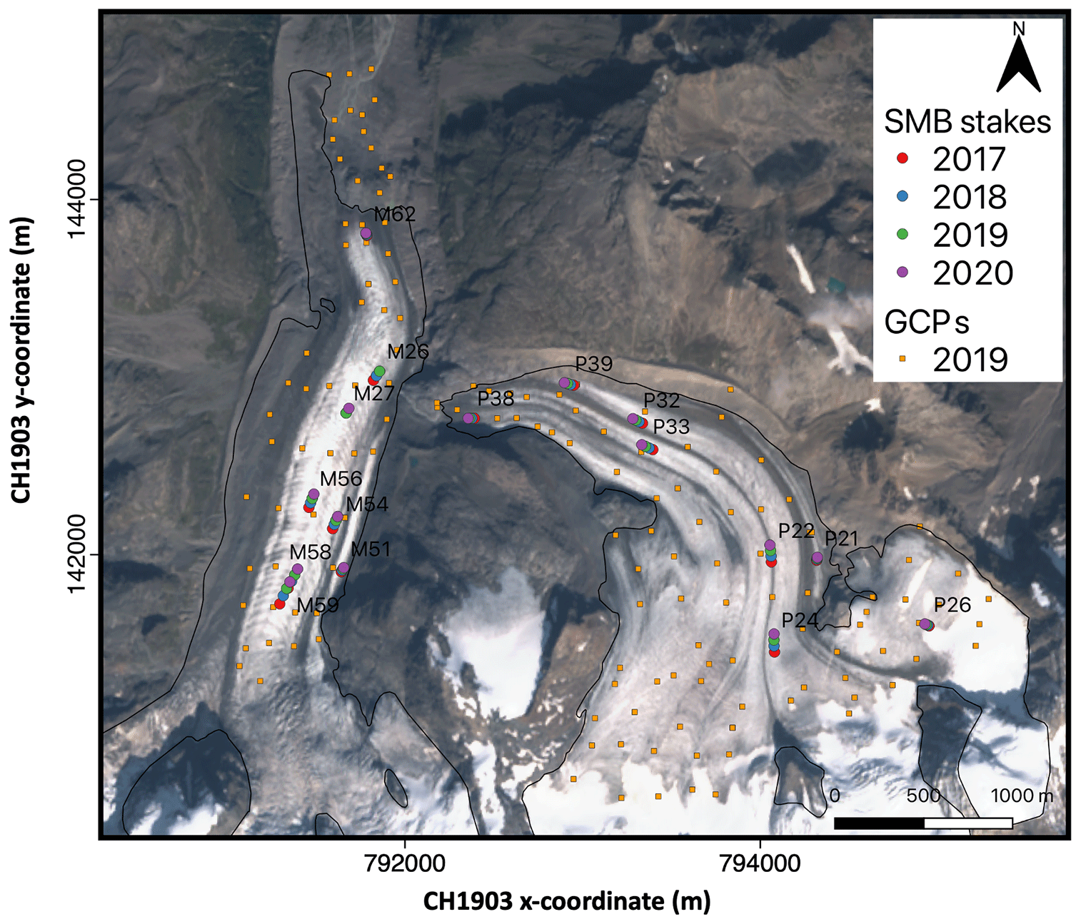
Figure 2Satellite image of the study area with the location of the measured ablation stakes in 2017, 2018, 2019 and 2020. The GCPs of 2019 are indicated with an orange square. The background image is a Sentinel-2 true colour composite satellite image from 13 September 2020. The different locations of the stakes in 2017, 2018, 2019 and 2020 show the movement of the stakes with the glacier flow. The labels refer to the stake names as used in the fieldwork programme. In 2019, stake M26, which was located in the middle of a crevasse field, was replaced by stake M27.

2.3 Ice thickness data

To calculate the local ice volume flux divergence (see Sect. 3.4), a distribution of the ice thickness is required. There are two published datasets of the ice thickness of the Morteratsch–Pers glacier complex, derived from radar measurements (especially in the ablation area) and modelling (especially in the accumulation area). The first one is the dataset of Zekollari et al. (2013), hereafter referred to as THIZ. This distribution was reconstructed by combining measured ice thicknesses (∼30 ground-borne ground penetrating radar (GPR) profiles in the early 2000s) with different modelling constraints. The second ice thickness distribution is the dataset of Langhammer et al. (2019), hereafter referred to as THIL. This distribution was produced by combining measured ice thicknesses (41 helicopter-borne GPR profiles with a total of 53 247 points measured in 2017) and modelling constraints with the Glacier Thickness Estimation (GlaTE) inversion scheme (Langhammer et al., 2019). We correct both datasets for glacier geometry changes to refer to the glacier state in 2018, 2019 and 2020, respectively, by subtracting the amount of local surface lowering. This concerns the local height difference between the UAV-created DSMs of 2018–2019–2020 and the DEM used for the respective ice thickness datasets. The latter are two DEMs provided by SwissTopo. DHM25 is valid for 1991 (used for THIZ), and SwissALTI3D is valid for 2015 (used for THIL).

Although both ice thickness distributions (Fig. 3a and b) have a similar pattern (location of overdeepenings, location of maximum ice thickness), large local differences exist (Fig. 3d). The ice thickness maximum, corrected to represent the ice thickness in 2020, for instance occurs at a similar location but is about 310 m for THIZ and 250 m for THIL. This corresponds to a difference of 18 %–24 %, which is, however, still within the error bounds of the datasets. Conversely, there are also certain zones (especially higher up Vadret da Morteratsch) where the difference between the two datasets is about 150 m.

Because of the significant differences between both ice thickness distributions, the choice for a particular distribution has a considerable effect on the calculations in this study. To verify the maximum ice thickness of Vadret da Morteratsch, we measured the ice thickness once again in the thickest region in 2020 (see Fig. 3c) with a Narod radio echo sounding (RES) system, similar to Zekollari et al. (2013) and Van Tricht et al. (2021). We preferred to use a low frequency of 5 MHz to limit the amount of attenuation due to disturbances in the glacier such as water inclusions, repeatedly observed during the fieldwork. We found a maximum value of 296 m, which is relatively close to the maximum thickness from the THIZ dataset. We can therefore certainly not ignore this dataset, despite the smaller number of measurements and the older date of creation. Therefore, for further calculations, we decided to use the mean ice thickness from THIZ and THIL at every grid cell, hereafter referred to as THIA (Fig. 3c). The effect of using THIA, as opposed to relying on THIZ or THIL, is examined as a part of the sensitivity analysis (see Sect. 5.1). For the areas where the current elevation is lower than the bedrock inferred from THIZ and THIL and where there is no ice as a result within the current glacier outline, we assume a minimal ice thickness of 5 m as in Zekollari et al. (2013).

Figure 3Ice thickness distribution of the ablation area of the Morteratsch–Pers glacier complex in 2020. (a) THIZ (ice thickness distribution of Zekollari et al., 2013), (b) THIL (ice thickness distribution of Langhammer et al., 2019) and (c) THIA (average ice thickness distribution). The difference between THIZ and THIL is shown in panel (d). Contour lines represent 50 m intervals. Note that at the front of Vadret da Morteratsch and locally at the front of Vadret Pers, the glacier outline is larger than the ice thickness dataset. The current surface elevation of these areas is lower than the bedrock elevation inferred from THIL and THIZ. The locations of the ice thickness measurements of 2020 are added in panel (c) with red circles. The background image is a Sentinel-2 true colour composite satellite image from 13 September 2020.

3.1 Continuity equation method

The continuity equation for glacier flow with constant density (Eq. 1) links the local mass balance (b) and the ice flux divergence per unit width in the local vertical ice column (∇⋅q) with local changes in the ice thickness ($\frac{\partial H}{\partial t}$), all expressed in m i.e. yr⁻¹ (see e.g. Hubbard et al., 2000; Berthier and Vincent, 2012).

Equation (1) shows that the difference between the local mass balance and ice flux divergence must be compensated by a change in local ice thickness. If the bedrock elevation is assumed to be constant, and compaction is negligible, which is the case in the ablation area (with ice throughout the entire column), the local ice thickness (H) in Eq. (1) can be replaced by the elevation of the surface (h). Further, because basal and internal mass balance in the ablation area are predominantly much smaller compared to the surface mass balance (b_s) (Kaser et al., 2003; Huss et al., 2015), b can be replaced by b_s, which after a reorganisation leads to the following expression:

By determining the local elevation changes (Sect. 3.2) and the components that make up for the ice flux divergence per unit width (from now on referred to as ice flux divergence; Sect. 3.3–3.4), the SMB pattern can then be derived.

3.2 DSM generation and surface elevation changes ($\partial h/\partial t$)

First, all the data from the UAV surveys are used to generate DSMs on a common local coordinate system (CH1903 + LV95). All the images collected during the UAV surveys are processed into orthophotos and DSMs using the photogrammetry workflow implemented in Pix4D. The accuracy of the reconstructed DSMs is assessed using the GVPs and the stable terrain outside the glacierised areas. Subsequently, surface elevation changes are directly computed from these DSMs by subtracting the DSMs from each other (2018–2017, 2019–2018, 2020–2019). Initially, all the DSMs are generated with a very high resolution of 0.05–0.09 m. But eventually, the surface elevation changes are resampled to 25 m resolution for further calculations using a block moving-average filter. This corresponds to the resolution of the ice thickness datasets and will therefore be the grid size for all of the following calculations.

A commonly observed feature on surface elevation change maps derived from high-resolution DSMs are alternating positive and negative differences. These are caused by the advection of local glacier topography such as crevasses, moulins, supraglacial melt streams, and large ice or rock boulders (Fig. 4) (Brun et al., 2018; Rounce et al., 2018; Yang et al., 2020). The above-mentioned variations are not caused by reduced or increased melt or accumulation and therefore need to be corrected for ice flow to make a correct SMB estimate.

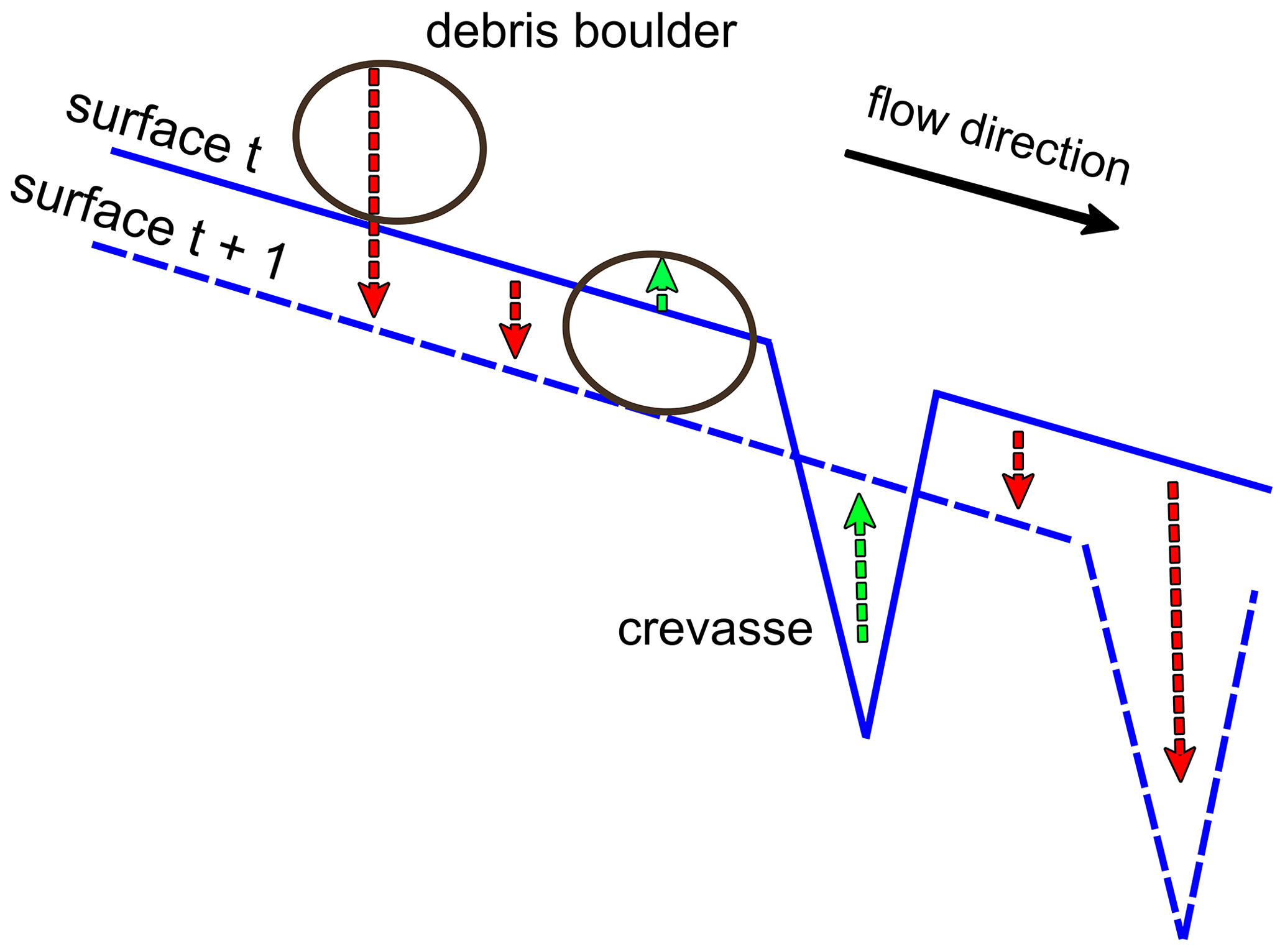
Figure 4The advection of surface topography (such as debris boulders and crevasses) can alter surface elevation changes between time step t and t+1 (red: negative $\partial h/\partial t$; green: positive $\partial h/\partial t$). The net effect on the surface elevation depends on the amount of lowering and the vertical extent of the moving features on the glacier surface.

Download

The different DSMs are treated considering the motion of the ice, following the method applied in e.g. Brun et al. (2018). This method consists of projecting each point on the glacier back to its original position in the previous year, based on the local velocity in the x and y direction and taking into account the vertical displacement produced by flow along the longitudinal slope. The latter is determined by taking the average slope over all the different years for which a DSM was made, smoothed with a Gaussian filter with a 25-pixel kernel size (50 m).

3.3 Horizontal surface velocity

Glacier surface velocities, which are needed to calculate the ice flux divergence (Sect. 3.4) and to flow-correct the surface elevation changes (Sect. 3.2), are computed for the 3 individual mass balance years. Velocity grids are derived by applying the Image GeoRectification And Feature Tracking (ImGRAFT) toolbox, an open-source tool in MATLAB (Messerli and Grinsted, 2015). Specific settings for the template matching of ImGRAFT are the use of the orientation correlation (OC) method and a large search height and search width of 200 m to guarantee that all possible areas are covered. Instead of using visual image data with variable illumination and snow cover, the feature tracking algorithm is run on hillshades (relief DSMs) of the original DSMs, resampled to a resolution of 2 m (Messerli and Grinsted, 2015). The latter turned out to improve the correlation success (Rounce et al., 2018).

Velocity maps are computed and corrected for differences in acquisition dates to obtain values in metres per year. Then, a series of filters are applied to the output of the cross-correlation to exclude poorly correlated pixels and those with unrealistic displacements or flow directions (Ruiz et al., 2015). The latter is a common issue for snow-covered areas, debris-covered areas or complex crevasse areas where no accurate displacements can be detected. As a first filter, after verifying average zero displacement for stable areas outside the glacier, all the computed velocity vectors outside the glacierised areas are removed by using the digitised glacier outlines (Heid and Kääb, 2012). The latter are manually digitised based on drone and satellite images and correspond to the end of the summer of every balance year under consideration. Then, a median filter is applied which removes velocity components that deviate too much from the surrounding vectors (Heid and Kääb, 2012; Nagy et al., 2019). Finally, we also impose a maximum velocity threshold derived from the modelled velocities in Zekollari et al. (2013), which are constrained with field observations. In other words, we limit the maximum surface velocity at every grid cell to the velocity modelled in Zekollari et al. (2013) + 20 %. The latter is a margin to take into account potential errors present in the study of Zekollari et al. (2013). However, after analysis this proved to not be necessary as these high values did not occur. The raw velocity maps containing gaps after filtering are then interpolated using a cubic spline interpolation (Ruiz et al., 2015). As validation, we compare the obtained velocities with measured velocities from stakes.

3.4 Ice flux divergence from ice thickness and surface velocities

The ice flux divergence (in m i.e. yr⁻¹) corresponds to the local upward or downward flow of ice relative to the glacier surface. It represents the difference between the ice supplied from upstream and lost downstream at a particular position. It is defined to be negative for upward motion (mass supplied to the surface, also referred to as the emergence velocity) and positive for downward motion (mass is removed from the surface, also referred to as the submergence velocity).

Different approaches exist to calculate the ice flux divergence, ranging from the use of 3D ice flow models (Seroussi et al., 2011; Vincent et al., 2021) to the use of simple geometric calculations and flux gates (Nuimura et al., 2011; Berthier and Vincent, 2012). The important distinction is the simplicity and the resolution with which they can be calculated. In this study, the ice flux divergence is computed for each grid cell by combining surface velocities and ice thickness according to Eq. (3):

The right side of Eq. (3) contains two horizontal ice flux components, of which the first corresponds to the ice thickness divergence and the second one to the velocity divergence (Reeh et al., 2003). Both are computed from the relevant derivatives. F is the depth-averaged glacier velocity ratio ($\overline{u}/u_{\mathrm{s}}$). For an isothermal glacier with negligible basal sliding and Glen's flow coefficient n=3, F is 0.8. However, the Morteratsch–Pers glacier complex is assumed to be a temperate alpine glacier complex which is accompanied by basal sliding. According to Zekollari et al. (2013), internal deformation accounts glacier-wide on average for 70 % of the flow and basal sliding for the remaining 30 %. However, in the ablation area the contribution of internal deformation is most likely even higher. Therefore, for the standard runs in this study, we take an F value of 0.9. However, the F value may vary locally (Zekollari et al., 2013), and varying this parameter will therefore be part of the sensitivity analysis.

3.5 Spatial scales of the ice flux divergence

In contrast to the surface elevation changes, for which the accuracy is expected to be high, the computed ice flux divergence is subject to larger uncertainties. This uncertainty directly relates to the large uncertainties in the reconstructed ice thickness field. Moreover, a considerable part of the uncertainty also originates from the spatial scales that need to be considered: due to longitudinal stresses, the local ice dynamics depend not only on the local glacier geometry (an assumption of the shallow ice approximation; see e.g. Hutter and Morland, 1984) but also on the surrounding geometry, typically over scales corresponding to several times the local ice thickness (accounted for in higher-order and full Stokes models; see e.g. Zekollari et al., 2014, where such a model was applied for this glacier complex). Local gradients of the ice thickness and the velocity are often magnified when they are determined on a numerical grid with a central difference scheme. This is directly reflected in the ice flux divergence pattern. Therefore, to make the ice flux divergence solution independent of the resolution and to take non-local stresses into account, larger scales must be considered (Reeh et al., 2003; Rounce et al., 2018). To date, studies applying the continuity equation method usually resampled the ice flux divergence grid to a much lower resolution (Nuimura et al., 2011; Seroussi et al., 2011; Rounce et al., 2018) or considered a flux gate approach (Berthier and Vincent., 2012; Vincent et al., 2016; Brun et al., 2018). However, as we aim for a high resolution of the SMB determination in this study and to obtain spatial variations in the ice flux divergence field, we opt to retain the 25 m resolution and to apply a filter to consider larger scales for the calculation of the ice flux divergence.

Different filters have been applied, of which most are constant box filters (e.g. mean, median) with a strong variation in size (up to 10 000 m) (Kääb and Funk, 1999; Seroussi et al., 2011; Rounce et al., 2018). Such filters give equal weight to cells within the box irrespective of their distance from the point in consideration (Kamb and Echelmeyer, 1986; Le Brocq et al., 2006). In this way, the effects of local phenomena (such as an ice fall or an acceleration in the glacier flow) are spread out uniformly when these filters are applied over larger distances, which implies that there are no localised peaks in the flux divergence field. Also, these filters have an abrupt cut-off point where the weighting becomes zero (Le Brocq et al., 2006). Furthermore, effects of perturbations in, for example, ice thickness have been demonstrated to fade out exponentially for ice flow (Kamb and Echelmeyer, 1986). Because of all these reasons, we apply in this study a local exponential decay filter (Eq. 4):

In Eq. (4), dist is the maximum distance of a cell which is taken into account in the exponential decay filter (set at 2.5 km), i and j are indices, and W represents the weight of a particular cell at position [x+i, y+j] (Le Brocq et al., 2006):

In Eq. (5), x and y are the coordinates of the point being filtered, while x^′ and y^′ are the coordinates of the weighted points, and sl is the scaling length and is a crucial parameter determining how fast the exponential filter fades. This parameter directly relates to the length scale over which the longitudinal stresses determine the local ice flow. Theoretically, this scaling length is in the range of 1–3 times the local ice thickness for valley glaciers and 4–10 times for ice sheets (Kamb and Echelmeyer, 1986; Le Brocq et al., 2006). For our experiments, we vary the scaling length depending on A times the local ice thickness (Eq. 6). In this way, we incorporate variations within the study area into the exponential decay filter, and we account for non-local flow coupling. The latter was shown to be an improvement compared to fixed-size filters (Le Brocq et al., 2006). As such, the ice flux divergence in areas with a larger ice thickness is considered over a larger distance compared to areas with a smaller ice thickness.

with

To provide for conservation of mass within our survey area, the filtered result in each grid cell is multiplied by the ratio of the net flux divergence (sum of all ice flux divergences) before and after filtering. To determine the optimal procedure to include the effects of (longitudinal) stresses and uncertainty in the input data, we perform multiple experiments with the exponential decay filter. For this, we examine whether (i) the ice flux divergence, (ii) the gradients of velocity and ice thickness, or (iii) both should be considered over larger spatial scales for optimal results in the determination of the SMB.

First, the ice flux divergence is considered over larger spatial scales by applying the exponential decay filter to the ice flux divergence field. Second, to compensate solely for the effects of large gradients, the gradients are considered over larger spatial scales. We therefore apply the exponential filter to the ice thickness and velocity gradients and calculate the ice flux divergence using these smoothed gradients. Third, to compensate for the negative effects of very large scaling lengths for both previous experiments and the biases related to both, we filter twice. Hence, both filters are applied after each other. In this way, the smoothness of the ice flux divergence field increases, while the top values are not damped as much as when applying a filter once with a long scaling length. This tends to reduce the distance over which the filtering must be performed, which is favourable to preserve local variations.

For every experiment, the modelled and measured SMB values at the position of the stakes are compared (see Sect. 2.2). As metrics to quantify the performance of the procedure, the mean absolute error (MAE) and the root mean square error (RMSE) are used (Eqs. 7 and 8). The MAE is defined as the absolute difference between the modelled and the measured SMB. The RMSE on the other hand takes into account the variance of the errors; n is the number of stake measurements. The uncertainty in the SMB measurements is estimated to be ±0.2 m i.e. yr⁻¹ and is also considered in the analysis. More specifically, for each filter option we carry out 100 versions in which we perturb the measured SMB. This is done by randomly adding a value between −0.2 and 0.2 distributed around 0. Then, for the option under consideration, the average MAE and RMSE are calculated from Eqs. (7) and (8), where n is the number of SMB measurements for every year (see Sect. 2.2), i is an index ranging from 1 to n (16), and x_i and y_i are the Cartesian coordinates of the different stakes under consideration.

4.1 Surface elevation changes and filtering

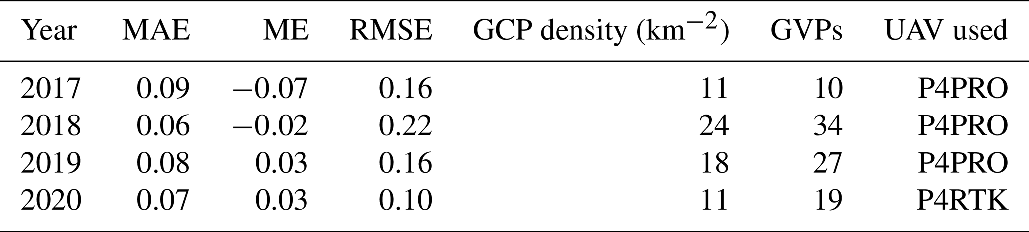
The accuracy of the elevation product is first assessed by comparing the photogrammetrically created DSMs with GVPs, randomly divided over the study area. MAE between measured and modelled elevation is on the order of a few centimetres (Table 2), which is similar to values found in other studies (Whitehead et al., 2013; Immerzeel et al., 2014; Wigmore and Mark, 2017; Zhang et al., 2019). As such, the accuracy of the created DSMs is high. Furthermore, the mean error (ME) is close to zero, which indicates that the created DSMs are not biased. For 2017, the slightly larger MAE is probably caused by a smaller number of GCPs combined with a reduced visual content because of fresh snow on the glacier surface. Further, the small MAE and RMSE of the DSM in 2020 highlight the advantage of using an RTK equipped with an RTK GPS (P4RTK) for which a smaller number of GCPs are needed to reach similar or better accuracies compared to a classic set-up (UAV without RTK correction).

Table 2Mean absolute error (MAE), mean error (ME) and root mean square error (RMSE) of the elevation differences between the DSMs and the GVPs in different years. Units are in m i.e. The GCP density is the number of GCPs per square kilometre, while the column of GVPs represents the total number of GVPs in each year.

Download Print Version | Download XLSX

Then, the accuracy of the surface elevation changes is assessed by comparing the elevation differences in rectangular areas outside the glacierised areas for two regions (see Fig. 6), where the topography is assumed to be mostly stable (Yang et al., 2020). The histograms for the 3 different balance years show that most of the differences range between −0.2 and 0.2 m, which indicates that there is no large absolute offset between the DSMs of the different years (Fig. 5). For region 2, we find a larger standard deviation (SD) for the 2017–2018 difference, which appears to be caused by a small horizontal shift, which produces larger elevation differences (both negative and positive) in this steeper area. For the more gently sloping glacier surface, the effects are negligible. The larger SD for the 2019–2020 difference in region 1 is caused by an area where a part of the bare surface was eroded by a melt river, producing a tail of negative elevation differences. In general, the above analysis reveals that the vertical uncertainties resulting from the DSM differencing are limited.

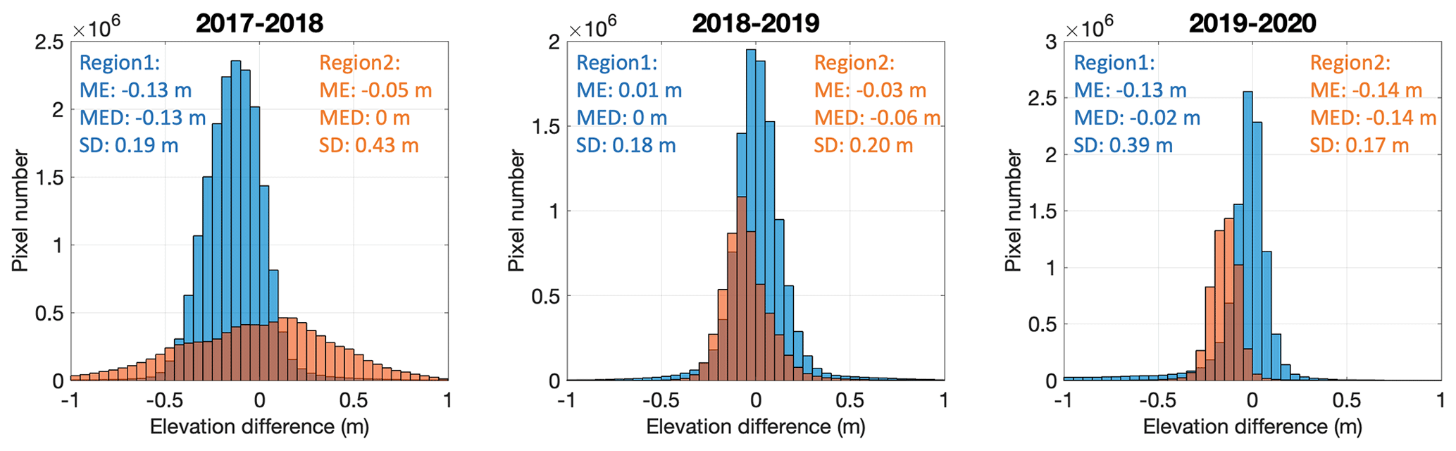
Figure 5Histograms of elevation differences for the different balance years considered. The mean error (ME), median error (MED) and standard deviation (SD) are added for each region. Regions 1 and 2 are defined in Fig. 6a.

Download

The different maps for the 3 balance years display a very detailed pattern of surface elevation changes (Fig. 6). For example, alternating positive and negative surface elevation changes are noticeable and can be explained by the advection of local glacier surface topography due to glacier movement (see also Fig. 4). In addition, significantly less negative $\partial h/\partial t$ values at the left side of Vadret da Morteratsch, especially where the glacier protrudes towards the north, are likely the result of a debris cover insulating the ice below and decreasing the melting rate (Reznichenko et al., 2010; Rounce et al., 2018; Rossini et al., 2018). The latter was also observed by the study of Rossini et al. (2018) focussing on the elevation differences on the front of Vadret da Morteratsch in the summer of 2016. Only at the terminal ice cliff can significantly higher $\partial h/\partial t$ values be observed (Immerzeel et al., 2014). Given that the ice fluxes can be assumed to remain relatively constant over the 3 years in consideration, the elevation changes indicate that 2017–2018 was the year with the most negative SMB (which is confirmed by field measurements) (see Fig. 11). Further, large positive surface elevation changes can be distinguished for 2019–2020 at the highest part of Vadret Pers. This is probably the result of avalanches originating from the steep accumulation area and persistent snow cover in these areas. This is striking as surface elevation changes farther down on the glacier are generally more negative compared to 2018–2019; i.e. the SMB gradient on Vadret Pers is steeper in 2019–2020 compared to 2018–2019.

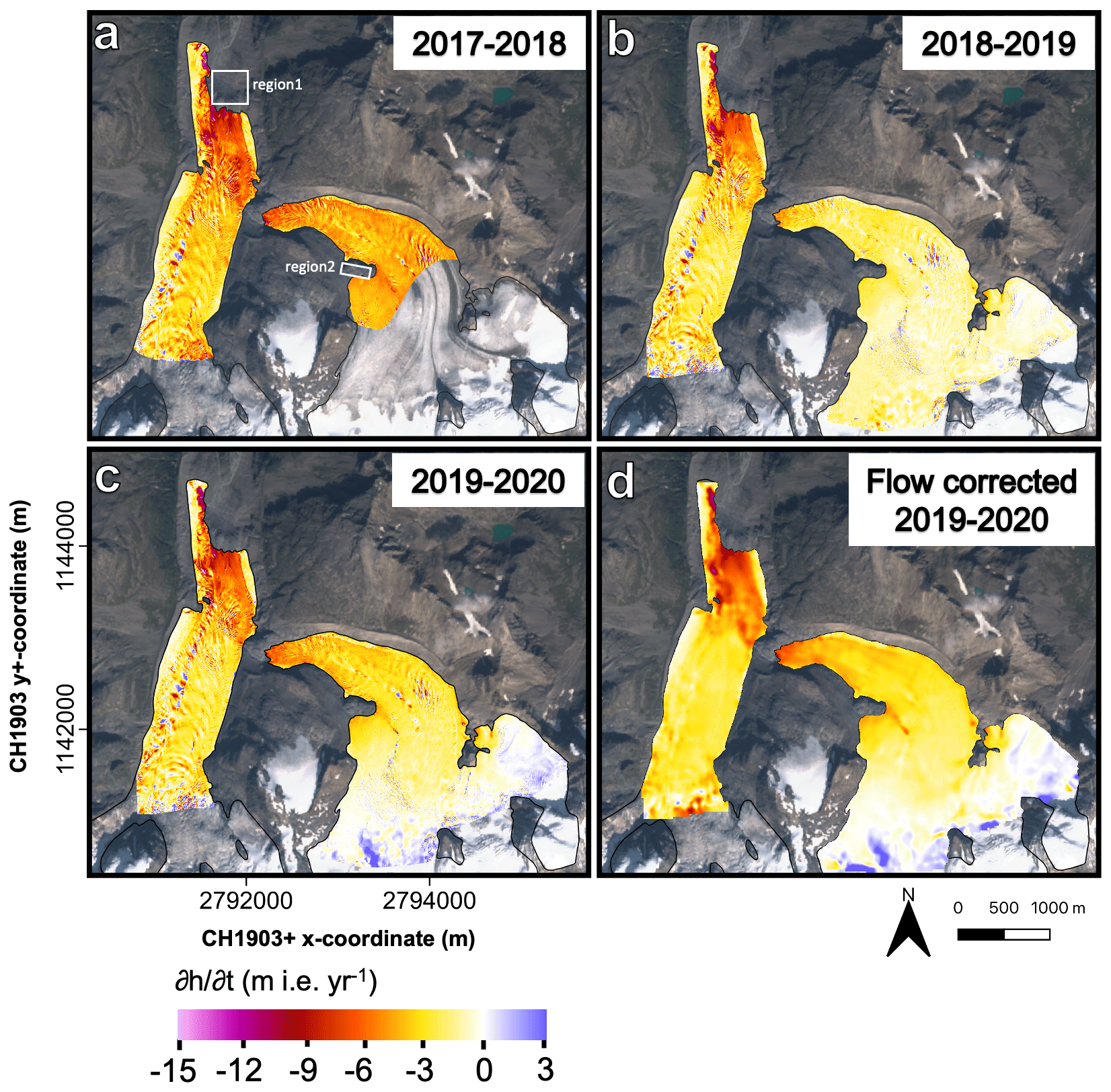
Figure 6Surface elevation changes for (a) 2017–2018, (b) 2018–2019 and (c) 2019–2020. The spatial resolution is equal to 8 cm. Panel (d) shows the surface elevation changes for 2019–2020 after flow correction. The outline of the glacier corresponds to the latest year of observation for every balance year in consideration. The two white boxes (region 1 and region 2) are stable areas which are used for the error analysis. The background image is a Sentinel-2 true colour composite satellite image from 13 September 2020.

Alternating positive and negative surface elevation changes are occurring, caused by the advection of surface topography (Figs. 4 and 6). We correct for these non-SMB features by flow-correcting the DSMs (see Sect. 3.2). The alternating pattern has clearly faded (Fig. 6d). At the top of the ablation area of Vadret da Morteratsch, near the ice fall, the $\partial h/\partial t$ values at the margin of the area are unrealistic because of inaccurate velocity calculations (see Fig. 7) and margin effects of the longitudinal slope. However, this area lies outside the area under investigation (see Fig. 7).

4.2 Glacier surface velocity

The velocity map derived from feature tracking and filtered for errors (see Sect. 3.3) contains several voids (Fig. 7a). This is caused by a lack of correlation between the 2 years, which is typically related to deformations of the surface, repositioning of supraglacial melt streams, and the presence of snow cover or debris. The latter hampers an accurate tracking between 2 consecutive years. To fill these gaps, cubic spline interpolation is used (Fig. 7b).

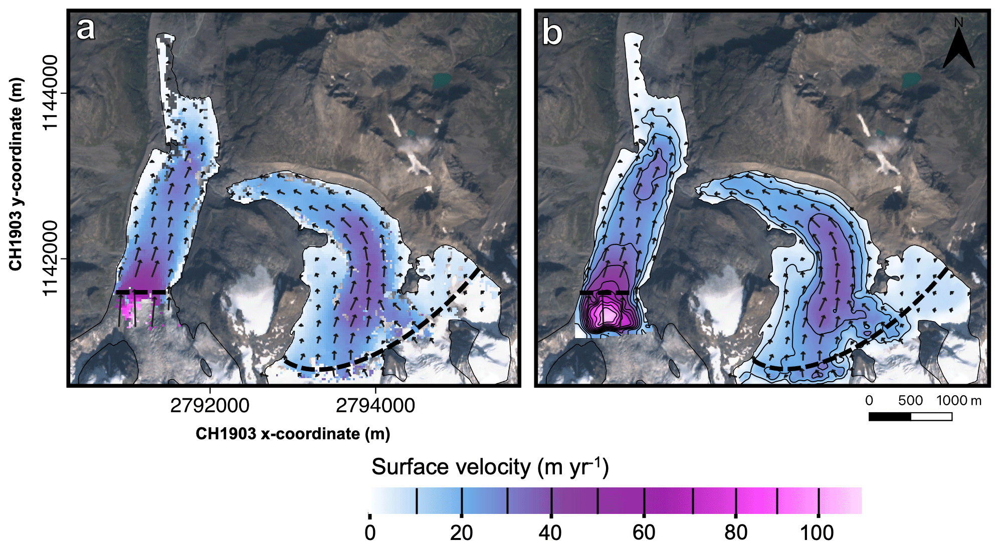
Figure 7Horizontal surface velocities derived from feature tracking between 2019 and 2020. (a) Filtered surface velocity, (b) void-filled filtered surface velocity. The black arrows indicate the flow direction. The dashed black line indicates the limit of the glacier area where the velocity is modelled without many gaps (area used for further analyses, e.g. when calculating ice flux divergences). The background image is a Sentinel-2 true colour composite satellite image from 13 September 2020. The contour lines are added for every 10 m yr⁻¹, and they are indicated in the colour bar.

Comparison with the velocities obtained by field measurements using ablation stakes (based on a high-precision RTK GPS system, estimated accuracy of approx. 0.1 m yr⁻¹) reveals a good agreement. We find the ME and RMSE to be 0.01/1.7 m yr⁻¹ for 2017–2018, 0.99/1.9 m yr⁻¹ for 2018–2019 and −0.37/1.8 m yr⁻¹ for 2019–2020 (Fig. 8).

Figure 8Comparison between surface velocities at stakes from field observations (high-precision GPS measurement at stakes) and from feature tracking.

Download

The surface velocities of 2017–2018 are higher compared to 2018–2019. Because the surface velocities in 2019–2020 also appear to be slightly larger compared to 2018–2019, it might be due to a larger amount of basal sliding in these 2 balance years. The latter can be caused by an increased supply of meltwater lubricating the glacier's base, which can be linked to a more negative $\partial h/\partial t$ in 2017–2018 and 2019–2020 compared to 2018–2019 (see also Fig. 6).

4.3 Ice flux divergence

After considering various spatial scales and filter procedures to determine the ice flux divergence, we find optimal results (lowest MAE, RMSE and minimal scaling length; see Sect. 5.2) when both filters are applied after each other for a scaling length of 4×H to smooth the ice thickness and velocity gradients and a scaling length of 1×H to smooth the ensuing ice flux divergence (see Sect. 3.5). These values are close to the theoretical values of the fundamental longitudinal scaling length for valley glaciers, mentioned in Kamb and Echelmeyer (1986). It shows that the data need to be considered over large spatial scales, which implies that the ice flux divergence field must be sufficiently smooth to give accurate results.

The computed ice flux divergence is clearly characterised by negative values over both glacier tongues (Fig. 9). This represents horizontal compression and associated vertical extension, which is generally expected for ablation areas (e.g. Kääb and Funk, 1999). This horizontal compression translates into an ice supply towards the surface (emergence velocity), which counters the effect of the negative mass balance on the local ice thickness change (and neutralises it in case the glacier is in equilibrium with the local climatic conditions). The ice flux divergence reaches a minimum between 500 and 1000 m from the terminus of the Vadret da Morteratsch, with values close to −4 m i.e. yr⁻¹ (Fig. 9). In this area, both the ice thickness (Fig. 3) and the surface velocity (Fig. 7) decrease significantly, which leads to large negative gradients and hence upward motion (negative ice flux divergence). It is therefore not surprising that there is a complex pattern of transverse crevasses in this area (see Fig. 2). The maximum ice flux divergence at the eastern side of Vadret da Morteratsch near the former confluence area with Vadret Pers is suspicious. This is likely caused by the very large ice thickness gradient because of the contribution of the underestimated ice thickness in the THIZ dataset. In this area, the THIZ dataset revealed zero ice thickness because of an overestimation of the bedrock elevation (Fig. 3).

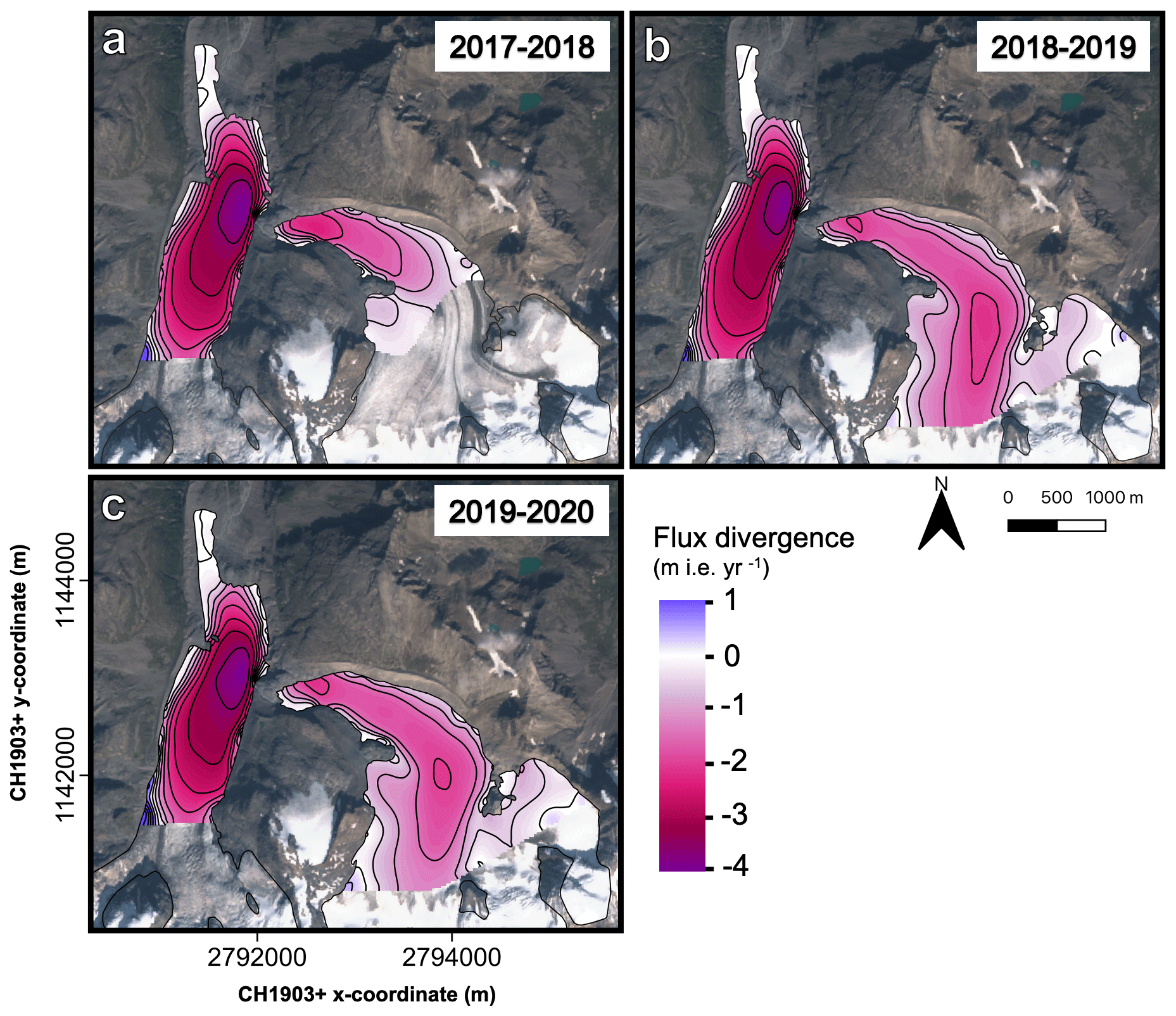
Figure 9Maps of the modelled ice flux divergence for the different years under consideration. Contours are added for every 0.5 m i.e. yr⁻¹. The background image is a Sentinel-2 true colour composite satellite image from 13 September 2020.

4.4 SMB from UAV

The final step of the method is to add the surface elevation changes (see Fig. 6) and the computed ice flux divergence (Fig. 9) to obtain the SMB (see Eq. 1). The final product, the modelled SMB for the 3 balance years, is shown in Fig. 10. The 3 years in consideration clearly show a rather similar pattern. Areas with a less negative SMB are located at the same locations (e.g. western margin of Vadret da Morteratsch). Areas with the most negative SMB are also at the same location (e.g. glacier fronts). The ice flux divergence is prominently not able to compensate for the very negative SMB so that there is net mass loss everywhere, and the elevation changes are less than zero. The most negative SMB (up to −13 m i.e. yr⁻¹) is found at the front of Vadret da Morteratsch in 2017–2018, which is in accordance with the SMB measurements. This concerns the lowest area, which is also quasi-stagnant with a very limited supply of ice from upstream (see Fig. 9). The presence of certain irregular patches with a smaller or larger SMB is caused by artefacts in the flow correction method (see Sect. 3.2 and Fig. 6d). This is because the flow correction method cannot trace all displacements exactly (rocks fall over, crevasses deform, supraglacial melt streams are positioned on different locations, etc.) because the velocity field is not fully accurate and because the calculation of the longitudinal slope also affects the result.

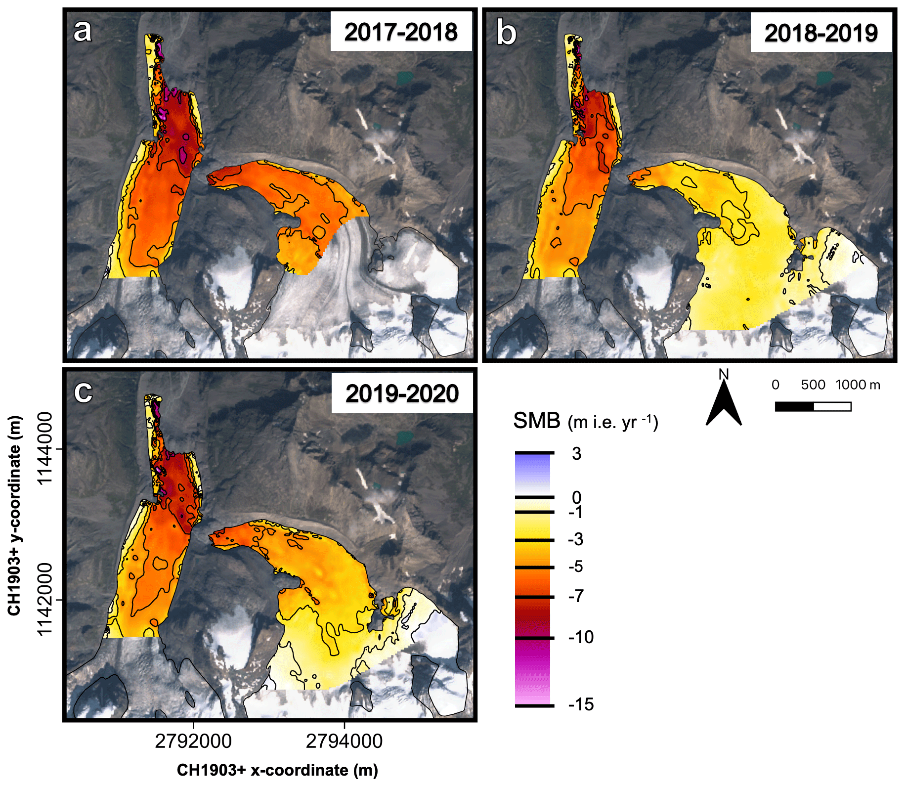
Figure 10Maps of the modelled SMB fields. Contours are added for specific values (indicated on the colour bar). The background image is a Sentinel-2 true colour composite satellite image from 13 September 2020.

The associated point-by-point comparison between modelled and measured SMB confirms the good match, with deviations generally smaller than 0.5 m i.e. yr⁻¹ (Fig. 11). Next to that, the ME is close to zero, indicating that the derived optimal SMB fields are not biased (Fig. 11). Only for Morteratsch in 2018–2019 is the ME slightly larger. The largest differences are found at the front of Vadret Pers (Fig. 11). Near the glacier front, the ice flux divergence is likely underestimated as a result of overestimated ice thickness in this area of the THIZ dataset. The latter decreases the ice thickness gradient in this area substantially.

In 2019, stake M26 (see Fig. 2) was replaced by M27 (and installed at a higher location) because it was located in the middle of a field of transverse crevasses during the survey in 2019. It is noticeable that this location was characterised by a more negative SMB compared to the surrounding areas in both 2017–2018 and 2018–2019 (see Figs. 10 and 11), which is probably caused by a more exposed position on an ice serac.

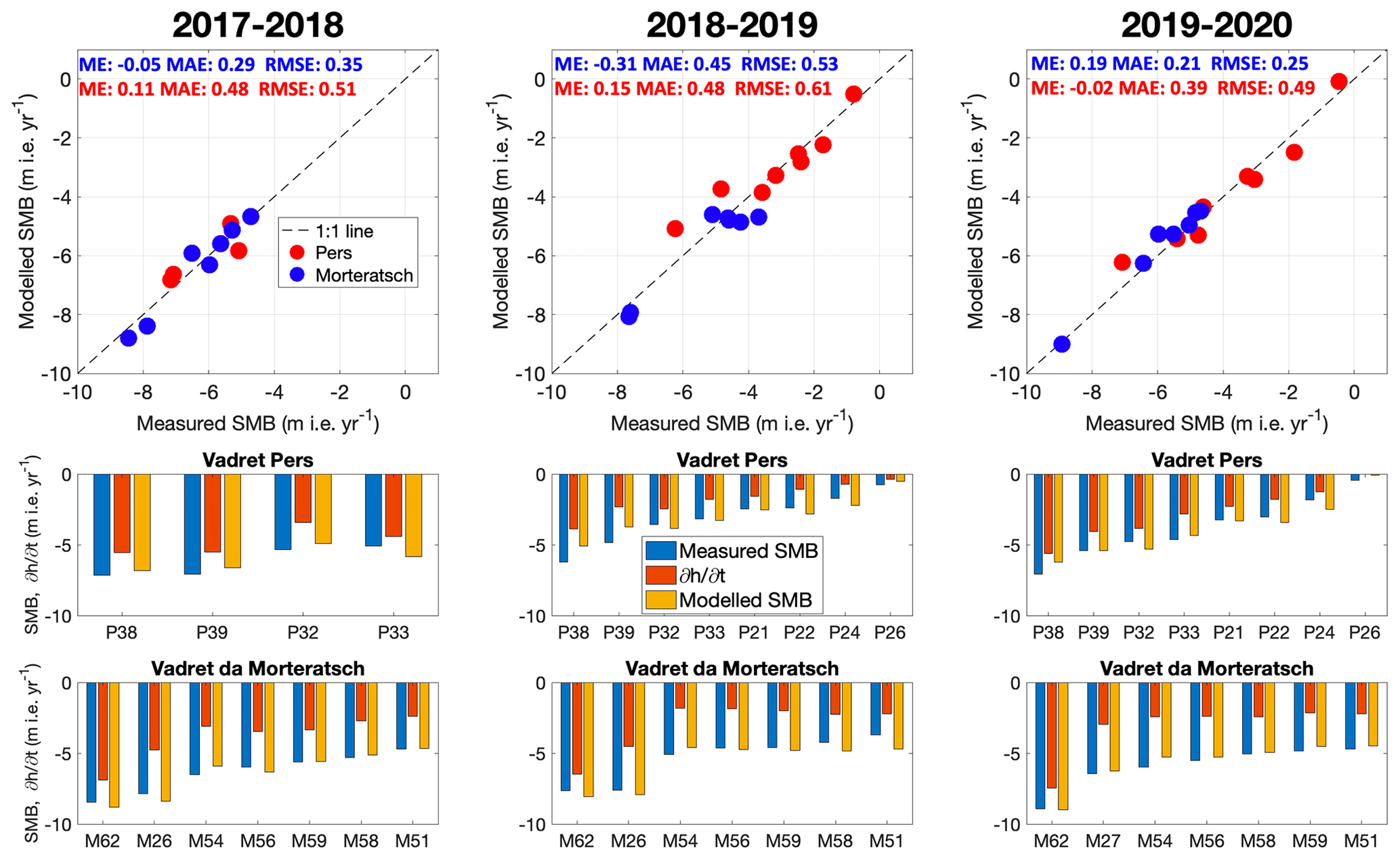
Figure 11Point-by-point comparison of modelled and measured SMB. In the lower panels, the difference between the modelled SMB (yellow bar) and the local elevation change (red bar) results from the modelled ice flux divergence. The labels refer to the stake names as used in the fieldwork programme. The ME, MAE and RMSE of the modelled SMB are added in the upper panels (values are in m i.e. yr⁻¹).

Download

For the optimal SMB fields, a minimum MAE of 0.21 m i.e. yr⁻¹ is obtained for Vadret da Morteratsch in 2019–2020 (Fig. 11). The MAE and RMSE are somewhat larger for Vadret Pers, with a maximum of 0.61 m i.e. yr⁻¹ in 2018–2019, which is mainly caused by the larger deviation for the lowest two stakes (Fig. 11).

4.5 Lateral variations in the SMB pattern

Using the continuity method based on close-range (UAV) remote sensing data clearly reveals a much more detailed picture of SMB than is possible from a stake network at a limited number of locations. This is evident in the lateral heterogeneity of SMB, which is often overlooked when considering elevation as the prime variable to plan the stake locations. In Fig. 12 the difference is shown between the UAV-derived SMB field and an SMB field only determined by elevation as derived from a linear fit of the stake measurements with altitude (see the inset of Fig. 12). In general, the largest differences occur close to the margin of the glaciers and around their front. The differences at the glacier margin of Vadret da Morteratsch are mainly related to a thick debris cover, which when sufficient in thickness has an insulating effect that reduces the glacier melt (e.g. Rounce et al., 2018; Verhaegen et al., 2020). For example, for the heavily debris-covered area where Vadret da Morteratsch protrudes towards the north, the SMB is −1.5 m i.e. yr⁻¹ below the debris and up to −12 m i.e. yr⁻¹ for the ice next to the debris. A thin layer of debris and the terminal ice cliff (Immerzeel et al., 2014) further reinforce the melt here, explaining this very high ablation rate (Rossini et al., 2018). The melt ratio is therefore equal to 0.125, which means that there is 87.5 % less melt under the debris at this location. This corresponds to a debris thickness of more than 50 cm when a typical average value of the characteristic debris thickness is used (Anderson and Anderson, 2016; Rounce et al., 2018). Such thicknesses are very likely in this area. During the fieldwork campaigns, boulder supply from the moraines was observed on several occasions, which was also documented in the Himalaya by Van Woerkom et al. (2019).

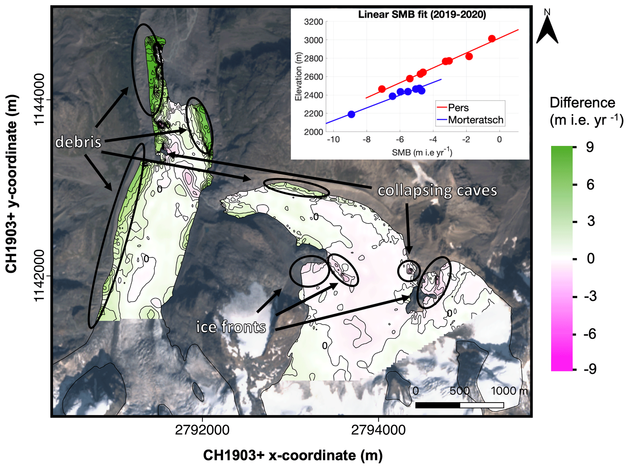
Figure 12The inset shows a linear SMB fit based on stake measurements. The main figure shows the difference between the UAV-derived SMB and the linearly derived SMB. The background image is a Sentinel-2 true colour composite satellite image from 13 September 2020. Contour lines are added for every metre. Labels are added for the contour of value 0 m i.e. yr⁻¹.

Another major feature is the presence of patches with a clearly more negative SMB when relying on the UAV-derived SMB field. These differences relate to stationary areas at local ice fronts or collapsing ice caves. While the first are real SMB variations (caused by more irradiation and/or less snow), the latter ones are not caused by the SMB. These collapsing ice caves clearly appear to occur near stagnant ice and at the bottom of the glacier, where meltwater forms a cave below the ice (Fig. 12). These caves collapse when the overlying ice becomes too thin due to melting at the surface. For the other areas, the difference between the SMB fields is generally smaller, between −0.5 and 0.5 m i.e. yr⁻¹. This is on the same order as the MAE and the RMSE and is slightly larger than the expected accuracy of the SMB measurements. The mean of the differences corresponds to 0.56 m i.e. yr⁻¹, which is specifically caused by the western side of the Morteratsch glacier, with a thick layer of debris (see Figs. 2 and 12). Using the simple linear fit to derive the SMB pattern would overestimate the ablation in the surveyed area by 2.4×10⁶ m³.

5.1 Dependence on the data and F value used

To study the dependence of the applied method on the uncertainty attributable to the used data and F value, we create 100 perturbed fields of the surface elevation changes, the surface velocity, the F value and the ice thickness. After that, we do the calculations, using the perturbed data for one dataset and the original data for the other ones. Next, the MAE of modelled versus measured SMB is calculated 100 times and for all years, and the standard deviation of this MAE is determined. For the analysis, the different input fields are perturbed using random patches with a diameter (uniformly distributed) between 50 m (local errors at grid level) and 500 m, with perturbation values normally distributed with a standard deviation of half the error estimate.

The uncertainty in the surface elevation changes is assumed to be correlated in space, i.e. depending on a pattern across the glacier (e.g. Fischer et al., 2015). Therefore, the $\partial h/\partial t$ fields are perturbed with perturbations of maximum 0.5 m (plausible maximum value for the multiannual $\partial h/\partial t$ from UAV data) (see Table 2). Regarding surface velocity, we use error estimates of 10 % of the observed velocity, similar to the expected accuracy (see Sect. 4.2). Besides velocity itself, the assumption of a constant F value is rather unrealistic (Zekollari et al., 2013). Ice flow over basal irregularities causes variations in F. Previous research showed for example F to be larger over basal highs and smaller over basal lows, and glacier areas with more basal sliding could also be characterised by a larger F value (Reeh et al., 2003). Therefore, we apply perturbations using an F value between 0.85 and 0.95. Concerning ice thickness, we apply perturbations with an error estimate of 30 %, taken from Zekollari et al. (2013).

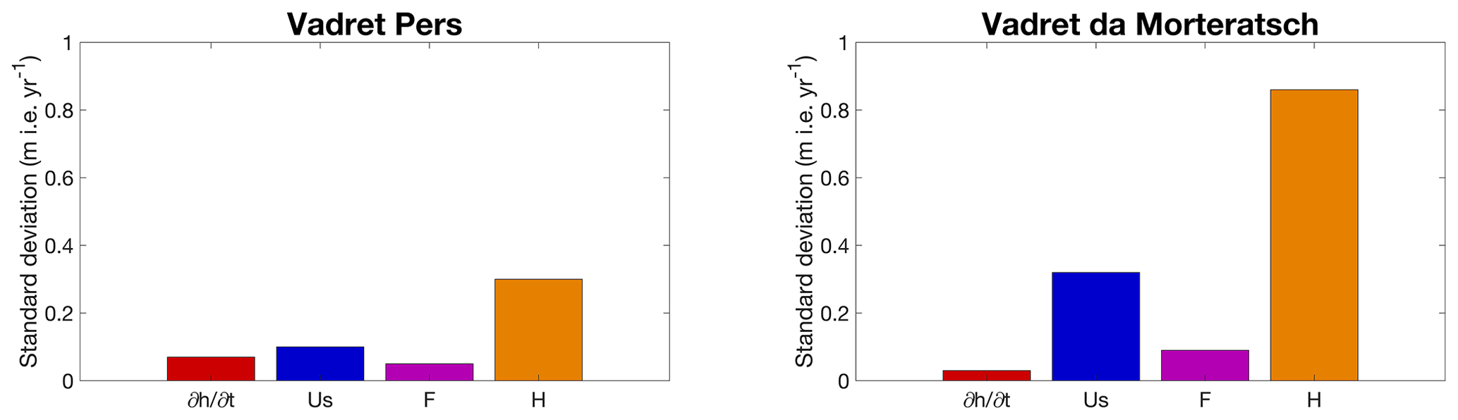
Figure 13Standard deviation of the MAE for the perturbed versions of the surface elevation changes, the surface velocity (u_s), the F value and the ice thickness (H).

Download

The effect of perturbation of $\partial h/\partial t$ on the determined SMB is small, with a standard deviation of less than 0.1 m i.e. yr⁻¹ for both glaciers (Fig. 13). As a result, the results of the applied method are not very dependent on (small) perturbations in $\partial h/\partial t$. Changes in the F value and surface velocity also appear to have minor sensitivity, especially concerning Vadret Pers. Regarding Vadret da Morteratsch, the applied perturbations of the surface velocity have an SD of the derived SMB of 0.3 m i.e. yr⁻¹, which is not negligible (Fig. 13). The ice thickness distribution, however, is for both glaciers undoubtedly most crucial for the determination of the SMB and even more so for Vadret da Morteratsch.

We therefore conducted some additional tests with both (THIZ and THIL) individual ice thickness datasets and for different combinations. For Pers glacier, the Langhammer dataset proved to be slightly better (MAE of 0.49 versus 0.60 m i.e. yr⁻¹), while for Morteratsch, the Zekollari dataset performed better (MAE of 0.74 versus 0.90 m i.e. yr⁻¹). But in general, all combinations tested gave poorer results, which encouraged us to use the average ice thickness in this study. Further, it should be mentioned that the above analysis is valid for the glacier-wide mean SMB deviations. For local point measurements, the uncertainty related to the used data or the F parameter might be larger.

5.2 Evaluation of procedures to filter the ice flux divergence

As the ice flow at a given location is determined by the surrounding glacier geometry (i.e. not only by its local geometry) and to avoid non-physical oscillations in the flux divergence field (as a result of fine grid spacing), it appears to be necessary to consider various spatial scales over which the ice flux divergence needed to be determined and different filtering procedures (see Sect. 3.5). The results of each possible combination are shown in Fig. 14.

By only applying the exponential decay filter to the ice flux divergence field (moving down in the matrix), we find minimum MAE and RMSE values when the scaling length is equal to 5 times H (MAE for Morteratsch–Pers is 0.51 m i.e. yr⁻¹). Such a large scaling length indicates that the ice flux divergence field must be smoothed significantly and therefore becomes entirely smeared with limited variation in the ablation area. One of the reasons for this high value are large ice thickness and velocity gradients resulting from solving ice flow processes on a high-resolution numerical grid. To compensate for the effects of large gradients, the second option is to consider the gradients over larger spatial scales. We do this by applying the exponential filter to the ice thickness and velocity gradients and calculating the ice flux divergence using these smoothed gradients (moving to the right in the matrix). A minimum MAE of 0.54 m i.e. yr⁻¹ is reached as soon as the velocity and ice thickness gradients are considered over 6 times H. The solution to compensate for the negative effects of a very large scaling length for both previous filters and the biases related to both is to filter twice, as is elucidated in Sect. 3.4 and shown in Sect. 4.3. As soon as the ice thickness and velocity gradients and the ice flux divergence are smoothed, the MAE becomes significantly smaller (Fig. 14). The MAE is now equal to 0.39 m i.e. yr⁻¹.

Figure 14Mean absolute error between measured and modelled SMB for various scaling lengths. The scaling length depends on the local ice thickness (×H). Smoothing of the ice thickness and velocity gradients (grad) and smoothing of the ice flux divergence (fdiv) are represented by the horizontal axis and vertical axis, respectively. M represents Vadret da Morteratsch, P represents Vadret Pers, and PM represents the entire glacier complex. The plots entitled “average” concern the average over all balance years. The selected combination with which the ice flux divergence is calculated as shown in Fig. 9 is encircled with black.

Download

Another observation standing out is that concerning Vadret Pers, the MAE mostly decreases when the ice flux divergence is smoothed, while for Vadret da Morteratsch, smoothing the gradients has a larger impact (see Fig. 14). Our explanation for these peculiar differences is that the gradients (both in terms of ice thickness and surface velocity) for Vadret Pers are already significantly smaller compared to those of Vadret da Morteratsch. The latter glacier has both a higher velocity and a larger ice thickness. Consequently, smoothing of the gradients for Vadret da Morteratsch is more decisive, whereas for Vadret Pers it is the other way around.

Other filters such as a mean filter or a Gaussian filter were explored, but all gave (slightly) less accurate results. However, our tests with a Gaussian filter showed only slightly larger errors for similar spatial scales. A Gaussian filter could therefore be a possible alternative to the exponential filter. Furthermore, the stakes used for validation were not entirely homogeneously distributed throughout the study area. The accuracy analysis may therefore have been biased towards these locations, which may also have influenced the choice of the optimal filter (length).