the Creative Commons Attribution 4.0 License.
the Creative Commons Attribution 4.0 License.
 | 25 Aug 2022
Four-dimensional temperature, salinity and mixed-layer depth in the Gulf Stream, reconstructed from remote-sensing and in situ observations with neural networks
Etienne Pauthenet
Loïc Bachelot
Kevin Balem
Guillaume Maze
Anne-Marie Tréguier
Fabien Roquet
Ronan Fablet
Pierre Tandeo
Despite the ever-growing number of ocean data, the interior of the ocean remains undersampled in regions of high variability such as the Gulf Stream. In this context, neural networks have been shown to be effective for interpolating properties and understanding ocean processes. We introduce OSnet (Ocean Stratification network), a new ocean reconstruction system aimed at providing a physically consistent analysis of the upper ocean stratification. The proposed scheme is a bootstrapped multilayer perceptron trained to predict simultaneously temperature and salinity (T−S) profiles down to 1000 m and the mixed-layer depth (MLD) from surface data covering 1993 to 2019. OSnet is trained to fit sea surface temperature and sea level anomalies onto all historical in situ profiles in the Gulf Stream region. To achieve vertical coherence of the profiles, the MLD prediction is used to adjust a posteriori the vertical gradients of predicted T−S profiles, thus increasing the accuracy of the solution and removing vertical density inversions. The prediction is generalized on a ∘ daily grid, producing four-dimensional fields of temperature and salinity, with their associated confidence interval issued from the bootstrap. OSnet profiles have root mean square error comparable with the observation-based Armor3D weekly product and the physics-based ocean reanalysis Glorys12. The lowest confidence in the prediction is located north of the Gulf Stream, between the shelf and the current, where the thermohaline variability is large. The OSnet reconstructed field is coherent even in the pre-Argo years, demonstrating the good generalization properties of the network. It reproduces the warming trend of surface temperature, the seasonal cycle of surface salinity and mesoscale structures of temperature, salinity and MLD. While OSnet delivers an accurate interpolation of the ocean stratification, it is also a tool to study how the ocean stratification relates to surface data. We can compute the relative importance of each input for each T−S prediction and analyse how the network learns which surface feature influences most which property and at which depth. Our results demonstrate the potential of machine learning methods to improve predictions of ocean interior properties from observations of the ocean surface.


In situ observations of the ocean vertical structure are accurate but sparsely distributed in time and space, hampering the study of mesoscale features (Siegelman et al., 2020a) and the computation of large-scale integrated variables such as ocean heat content (Wang et al., 2018; Durack et al., 2014). Meanwhile, the ocean surface has been observed at high temporal and spatial resolution with satellites since the early 1990s. Remote sensing allows us to observe surface signature of mesoscale to submesoscale features (Siegelman et al., 2020b) and to track climatic trends of sea surface height (Nerem et al., 2018), temperature (Merchant et al., 2019) and salinity (Reul et al., 2020). It is therefore highly valuable for combining sparse in situ profiles and high-resolution remote sensing observations in order to predict the ocean stratification at higher resolution and frequency.
This problem can be approached from two main points of view. First, the physical approach aims at constraining a global circulation model with all observations available (e.g., Lellouche et al., 2021; Forget et al., 2015). The numerical models have the advantage of offering a product that is physically consistent but that can contain drifts and biases (Stammer, 2005). The data assimilation is a practical means of reducing the spurious model drifts and biases, but still the model can diverge from observations and even drift in uncharted states in poorly sampled regions (Forget et al., 2015). Second, the statistical approach aims at finding the empirical relationship between the surface ocean and the interior. The simplest method is to use a multiple linear regression between sea-level anomaly (SLA), sea surface temperature (SST) and T−S profiles (Guinehut et al., 2012; Jeong et al., 2019). According to Guinehut et al. (2012), this method can only reconstruct 50 % to 30 % of the temperature and 20 % to 30 % of the salinity at depth. An improvement of the linear reconstruction method is to first reduce the T−S profiles and to link up the reduced variables to the satellite data. Indeed, it was found that only a few modes are needed to explain most of the variance or covariance of the temperature fields (Meinen and Watts, 2000) or of combined T−S profiles using the gravest empirical mode (GEM) projection (Sun and Watts, 2001). The GEM technique is a projection of hydrographic profiles onto a geostrophic stream function plane, which was used to estimate the four-dimensional structure of the Southern Ocean (Meijers et al., 2010). However, this requires that each dynamic height be associated with just one T−S profile at each longitude, meaning that outside of the Antarctic Circumpolar Current or boundary currents, the approach is questionable. Buongiorno-Nardelli and Santoleri (2005) developed the multivariate Empirical Orthogonal Function Reconstruction (mEOF-r) based on a similar idea. It is a linear system that uses surface data to predict the three leading modes of the EOFs applied to profiles of temperature, salinity, and geopotential thickness. They later showed that mEOF-r is outperformed by an artificial neural network for the North Atlantic region (Buongiorno Nardelli, 2020).
Machine learning approaches are increasingly used to deal with the ever-growing stream of geospatial data (Reichstein et al., 2019; Sonnewald et al., 2021; Wang et al., 2019). More specifically, deep learning methods are characterized by artificial neural networks (NNs) involving usually more than two hidden layers. They exploit feature representations learned exclusively from data (Zhu et al., 2017). Multiple studies recently presented deep learning methods for reconstructing hydrographic profiles from satellites. Proof-of-concept papers established the important capabilities of self-organizing maps (SOM; e.g., Charantonis et al., 2015; Gueye et al., 2014) and feed-forward or long short-term memory (LSTM) neural networks for hydrographic profile predictions (e.g., Lu, 2019; Jiang et al., 2021; Contractor and Roughan, 2021; Buongiorno Nardelli, 2020; Su et al., 2021; Sammartino et al., 2020). NNs can also efficiently reconstruct Argo interpolated fields (Gou et al., 2020; Meng et al., 2021). A recent study focused on predicting the mixed-layer depth (MLD) from satellites using probabilistic machine learning (Foster et al., 2021). However, to our knowledge these deep learning studies do not explore the vertical coherence of the predicted profiles, i.e., the presence of density inversions and the accuracy of the MLD prediction. The presence of density inversions makes an ocean product more difficult to use to initialize regional forecast models. Statically unstable profiles have to be removed when using the product to analyse ocean dynamics (e.g., New et al., 2021). The accuracy of the MLD prediction also has large implications for the pertinence of an ocean product. Indeed, the MLD and the strength of underlying stratification regulate the rate at which the ocean exchanges heat and gas with the atmosphere, which directly impact our climate (Sallée et al., 2021). To understand and quantify ongoing climate changes, we need to document the variability of the vertical gradients of temperature, salinity and density in the water column. Physically consistent products, in the spirit of the MIMOC climatology (Schmidtko et al., 2013) but with higher resolution in time and space, are required to validate models used for climate projections. In particular, western boundary currents such as the Gulf Stream play a major role in climate variability by carrying warm and salty near-surface waters northwards (Smeed et al., 2018) and by deeply impacting the atmosphere (Minobe et al., 2008). In the present paper we focus on the Gulf Stream region for its challenging high variability and its dense in situ sampling coverage.
Here we present a method to estimate the ocean stratification from surface data and the associated confidence intervals using a prediction model fitted with in situ historical data. We train a NN to predict temperature and salinity (T−S) profiles down to 1000 m and the MLD, in the Gulf Stream region, from satellite data covering 1993 to 2019. Our goal is to combine MLD, T and S predictions to produce T−S profiles that are physically consistent. Model training is done on raw in situ profiles alone (not interpolated fields), and predictions are generalized on a grid with ∘ horizontal resolution and daily time steps. Our framework further delivers a quantification of uncertainties through a confidence interval of the model prediction as well as the relative importance of each input variable. The proposed reconstruction method and resulting product are named OSnet for Ocean Stratification network.
The paper is organized as follows. Section 2 introduces the datasets used as inputs and outputs of OSnet as well as the products used as a benchmark to evaluate the performance of our reconstruction. Section 3 presents the method composed of the neural network and the MLD adjustment. Section 4 evaluates the accuracy of OSnet predictions and presents property maps and sections. OSnet profiles are compared to a mooring; we also compare time series and an analysis of the relative importance of each input for each output. In Sect. 5 we explore the potential of OSnet by estimating profiles from synthetic satellite data. Our conclusions are presented in Sect. 6.
2.1 Temperature and salinity in situ profiles
We use the in situ temperature and salinity (T−S) vertical profiles sampled by Argo floats (Argo, 2022) and ships from the CMEMS quality-controlled Coriolis Ocean Dataset for Reanalysis (CORA) database (Cabanes et al., 2013; Szekely et al., 2019). We keep only the profiles extending at least from 25 to 1000 m for the period 1993 to 2019, totaling 67 767 T−S profiles for the region 80 to 30∘ W and 23 to 50∘ N. All the profiles that do not reach 1000 m or start deeper than 25 m are discarded. Profiles are interpolated on an uneven vertical grid with 51 levels, with spacing increasing with depth (27 levels are within the first 100 m leading to a vertical resolution of 1 m in the upper levels and 450 m at 1000 m depth). Profiles without data at the surface are extrapolated by repeating the shallowest observation point. There is little seasonal bias in the distribution of data with 5647 profiles by month on average, a minimum of 5027 in February and a maximum of 6257 in October. The spatial distribution of profiles kept in the analysis is shown in Fig. 1b. It reveals a general lack of data in the center of the subtropical gyre compared to the Gulf Stream region west of 60∘ W. The temporal distribution (Fig. 1a) reveals a significant increase in sampling after 2000 thanks to the Argo program (Wong et al., 2020). After 2012, the number of T−S profiles stabilizes at ∼ 400 profiles per month.
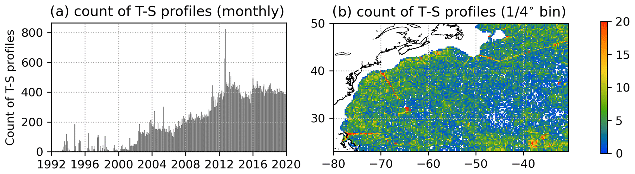
Figure 1Count of temperature and salinity profiles extending from 25 to 1000 m for the region. Profiles are counted for ∘ bins (b) and represented where they exceed 0 with a truncated color bar at 20 profiles; the maximum number of profiles for a bin is 185 profiles. The count in (a) is by months.
2.2 Input data
Input data (Table 1) are surface satellite data and bathymetry. Mean dynamic topography (MDT) is from the Centre National d'Etude Spatiale (CNES-CLS18) (Mulet et al., 2021), and the bathymetry is the ETOPO1 bedrock, distributed by NOAA (2009). The SLA is the level-4 daily product from CNES-CLS (6.2_DUACS_DT2018). It has a ∘ horizontal grid resolution. We also use geostrophic surface velocities derived from the SLA and distributed by CNES-CLS (Table 1). MDT is calculated by merging information from altimeter data, GRACE, and GOCE gravity field and oceanographic in situ measurements (drifting buoy velocities, hydrological profiles) (Mulet et al., 2021), while SLA is from altimeter data only. Keeping MDT and SLA separated in the inputs allows us to determine their respective importance in the prediction (see Sect. 4.4). The SST is from the European Space Agency (ESA) Climate Change Initiative (CCI) and Copernicus Climate Change Service (C3S), v2.3 and level-4 product. It provides gap-free maps of daily average SST at 20 cm depth and 0.05∘ × 0.05 ∘ horizontal grid resolution, using satellite data from the Along Track Scanning Radiometer (ATSR), Sea and Land Surface Temperature Radiometer (SLSTR) and Advanced Very High Resolution Radiometer (AVHRR) series of sensors (Merchant et al., 2019).
(NOAA, 2009)(Mulet et al., 2021)(Good et al., 2019)(Boutin et al., 2021)(Guinehut et al., 2012)(Lellouche et al., 2021)Table 1List of input variables for the neural network and additional datasets to compare with. ESA CCI: European Space Agency Climate Change Initiative. C3S: Copernicus Climate Change Service. NOAA: National Oceanic and Atmospheric Administration. DUACS: Data Unification and Altimeter Combination System. CMEMS: Copernicus Marine Environment Monitoring Service.
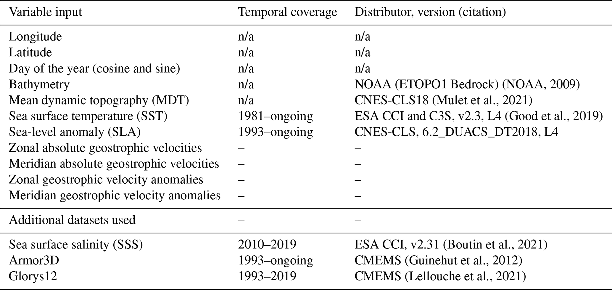
n/a: not applicable.
2.3 Additional datasets
We validate our results against other observational and synthetic datasets. The sea surface salinity (SSS) CCI dataset is distributed at ∘ horizontal grid resolution from 2010 to 2019 (Boutin et al., 2021). We do not use SSS as an input variable for several reasons. SSS satellite observations only cover the period 2010–2019, and its quality is questionable at high latitudes and in cold water (Boutin et al., 2021). As our prediction only depends on the input variables, it is risky to rely on data with systematic errors. Moreover, we tested an architecture with SSS as input, and results were not improved significantly: only the surface salinity was slightly better. The relative importance algorithm also showed that SSS was not used significantly in predictions. It has the same order of importance than geostrophic currents (see Sect. 3.4 on the explainability of the NN). However, SSS is a useful product to compare with, and we further discuss this in Sect. 4.5 and Appendix B.
We compare OSnet gridded fields to Armor3D and Glorys12 because they are the only ocean products, to our knowledge, that extend from 1993 to today with a spatial resolution of at least ∘ and a frequency under the month (weekly for Armor3D and daily for Glorys12). The global eddy-resolving reanalysis Glorys12 (Lellouche et al., 2021) is based on the physical model NEMO (Madec, 2015) and ocean observations assimilated by means of a reduced-order Kalman filter. It is provided at horizontal grid resolution and a daily mean. We also compare our results to the observation-based Armor3D weekly product (Guinehut et al., 2012). This later product is built in two steps: (i) prediction of synthetic T−S fields by multiple linear regression from SST and SLA and (ii) optimal interpolation combining synthetic and in situ T−S profiles. A section of OSnet is compared to hydrographic section AT20 sampled along 52.3∘ W by the research vessel Atlantis from 1 to 11 May 2012 (McCartney, 2012). Finally, we use T−S data sampled at moorings of the Line W array, deployed in April 2004 between Cape Cod and Bermuda. We use profiles from the third mooring located at 69.11∘ W, 38.51∘ N.
The method is composed of three steps (Fig. 2). Firstly, a neural network is trained to predicts T−S profiles and MLD from satellite data. Secondly, an adjustment of predicted T, S and MLD corrects the vertical shape of the profiles towards a physically consistent solution. Finally, an operational phase uses the trained network and MLD adjustment to predict T, S and MLD on daily grids from the satellite data.
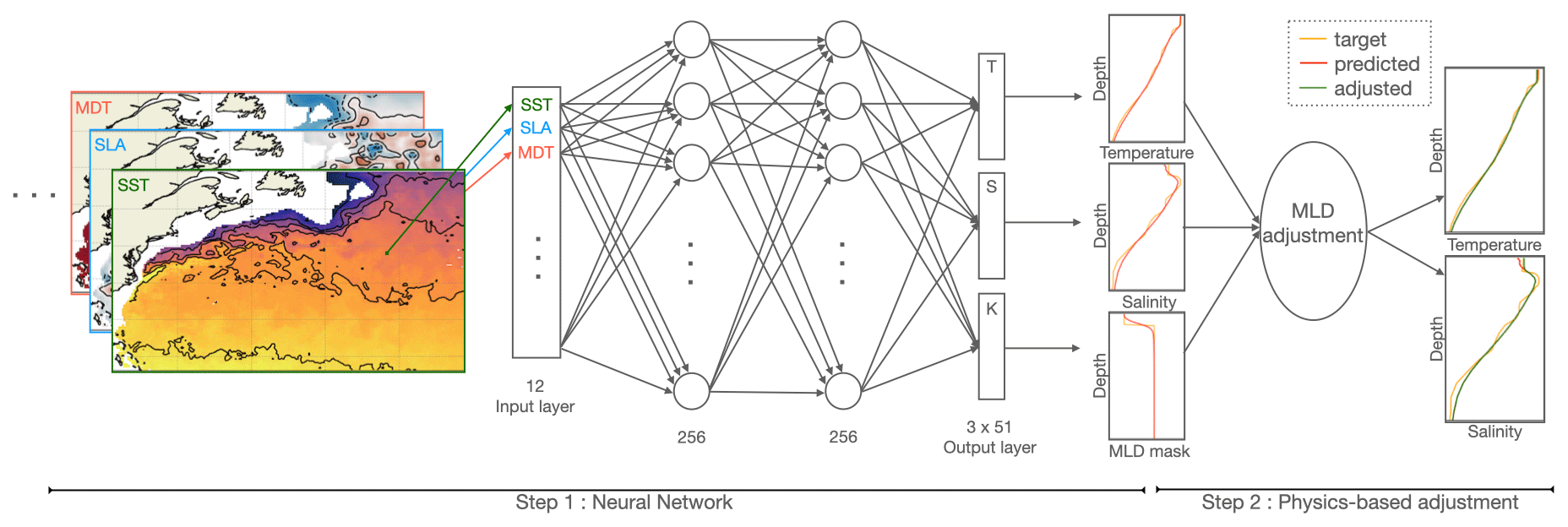
Figure 2Schematic of OSnet formed of a neural network (NN) with two hidden layers and a mixed-layer (MLD) depth adjustment. The NN uses 12 surface inputs that are listed in Table 1 to predict profiles of temperature (T), salinity (S) and MLD mask (K). T−S profiles are then adjusted using the profile K for a better prediction of the MLD.
The procedure is coded in Python with the help of several useful modules. The NN algorithm is coded with Tensorflow (Abadi et al., 2016) and the Keras application programming interface (Chollet and Others, 2015). It is explained with Shap (Kaur et al., 2020). Xarray (Hoyer and Hamman, 2017), Dask (Rocklin, 2015) and Numba (Lam et al., 2015) are used for fast computation and the management of large datasets. The color palettes for maps are from Cmocean (Thyng et al., 2016) and Colorcet (Kovesi, 2015). All the codes to build OSnet models are available at https://github.com/euroargodev/OSnet (last access: 27 June 2022, Pauthenet et al., 2022b), and the models and prediction tools specific to the Gulf Stream region are available at https://github.com/euroargodev/OSnet-GulfStream (last access: 27 June 2022, Pauthenet et al., 2022c).
3.1 The multilayer perceptron
The neural network used is a multilayer perceptron (MLP), which is a class of feed-forward artificial neural networks (Rosenblatt, 1961; Gardner and Dorling, 1998). The MLP guesses the non-linear relation between inputs and outputs, through one or more hidden layers with many neurons stacked together. The learning mechanism that allows the MLP to iteratively minimize the loss function is called backpropagation. We keep the architecture simple with only two layers of 256 neurones each. Dropout is used as a regularization method to reduce overfitting and improve generalization (Srivastava et al., 2014). Activation functions are a rectified linear activation function (ReLU) for the hidden layers, linear for T and S output, and a sigmoid for the MLD output. We tested more complex architectures (additional layers, convolutional layers, bottleneck architecture) but could not improve the accuracy of the results with them. A simple architecture is advantageous for its lower computation time. The input consists of 12 values, listed in Table 1: latitude, longitude, day of the year (cosine and sine), bathymetry, MDT, SST, SLA, four geostrophic velocities U, V and both anomalies. Inputs are linearly interpolated at the in situ location of each profile. The outputs are predictions of three vectors of 51 depth levels (temperature, salinity and the MLD mask). The depth levels are the ones presented in the data section, on which the CORA profiles are interpolated.
The dataset is split (randomly with no replacement) as follows: 20 % of the profiles are set aside for testing. In the remaining 80 %, we use 80 % as training data and 20 % as validation data. Validation data are used to avoid overfitting by assessing the performance of the trained model after each epoch (one epoch sees all the training data). Be aware that the train and test data are not truly independent: the selection is random without accounting for spatial and temporal autocorrelation. Once the training of the NN is finished, we select the model with the best performance on the validation dataset. We then run this model on the test dataset (data not seen in training or validation) to confirm the good generalization of the model (i.e., training and test errors are similar, Fig. 3). Given a NN architecture with good generalization properties, we retrain a NN using all 67 767 profiles (Fig. 3, orange) as training data. The training of one model takes ∼20 min on an eight-core CPU with 32 Go of RAM.

Figure 3Normalized root mean square error (nRMSE) between temperature (a) and salinity (b) observed (CORA) and predicted profiles (Glorys12, Armor3D, NN and OSnet). The normalization is done with the standard deviation of the observed temperature and salinity by depth. The upper panels are a zoom of the first 100 m of the full-depth lower panels. The Glorys12 (blue) and Armor3D (purple) profiles are collocated with the CORA profiles, and the error is calculated between these subsamples. The NN profiles are only predicted with the NN, without adjustment of MLD, for 15 trained datasets (dark grey) and 15 test datasets (light grey). NN full (orange dotted) corresponds to the predictions using the full dataset (test + train) and is averaged for 15 models (bootstrap). Finally, the OSnet profiles (orange) are predicted with a NN bootstrapped 15 times and the MLD adjustment is performed, which slightly increases the error at the surface.
To further improve the prediction performance and assess the associated confidence intervals, we exploit a bootstrapping scheme (Breiman, 1996). More precisely, we bootstrap the training procedure 15 times using a different initialization and training dataset each time. Indeed, because of the instability of the prediction method, bootstrapping can give substantial gains in accuracy. Overall, given 15 trained models, we compute the mean T, S and K profiles for all input data and their standard deviation (Fig. 3, grey). The latter delivers an estimate for the confidence interval. This bootstrap method reduces the estimation bias. Finally, the T−S prediction is generalized on a daily ∘ horizontal grid. The spatial resolution of the input data (Table 1) is unified to ∘ in longitude and latitude by a nearest neighbor interpolation method. This produces T and S fields with 51 depth levels from the surface to 1000 m for each day between 1 January 1993 and 31 December 2019. It is freely available (Pauthenet et al., 2022a).
3.2 Prediction of the mixed-layer depth
We define the mixed-layer depth H with a density deviation from the surface method, as proposed by de Boyer Montegut et al. (2004). It is the depth at which the potential density referenced to the surface, σ0, exceeds by a threshold of 0.03 kg m−3 the density of the water at 10 m, σ0 () =σ0 ( m) +0.03 kg m−3. This definition is chosen for its simplicity of application but tends to overestimate deep winter MLDs compared to the more sophisticated hybrid algorithm of Holte et al. (2017). These regions of deep winter MLD are rarely observed in our dataset (1145 profiles with MLD deeper than 300 m, i.e., 1.7 % of the dataset), comforting our choice of using a simple density threshold. For the NN, the mixed layer is represented in the form of a unitless profile K of size Z=51 that is filled with zeros between the surface and the mixed-layer depth H and with ones from H to −1000 m.
This formulation allows the NN to give an estimation of the gradients around the MLD instead of a single depth value (Fig. 4d). The resulting mask K is also convenient for the MLD adjustment performed on predicted profiles.
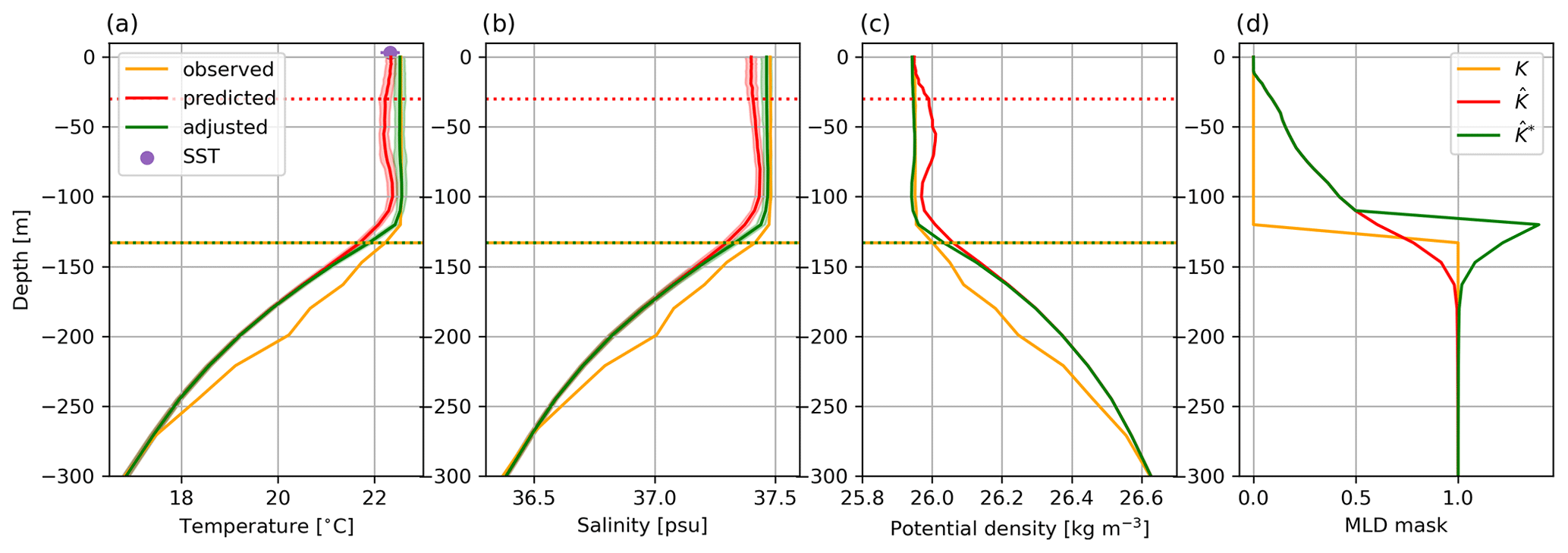
Figure 4Example of a profile (orange) sampled on 3 March 2012 at 35.55∘ W and 23.53∘ N, truncated at 300 m deep. We display temperature (a), salinity (b), potential density (c) and profile K that is a mask of MLD (see Eq. 1). The T−S profile predicted by the NN is in red and the adjusted using the profile (OSnet) in green (see Sect. 3.3). The green and red bands are the confidence interval for each profiles, i.e., the standard deviation of the 15 bootstrapped models. MLDs observed, predicted and adjusted are shown with dotted horizontal lines. SST is added with a purple dot and a horizontal bar for its mapping uncertainty.
3.3 Adjustment of the mixed layer
We identified two types of error in the direct prediction of T−S profiles. Firstly, the MLD predicted by the profile has a better accuracy (MLD RMSE of 40 m) than the MLD computed from the T−S profiles directly (MLD RMSE of 50 m). The latter is systematically too shallow due to unrealistic T−S excursions on the vertical in the mixed layer, causing the density threshold to be reached too close to the surface. These sharp variations of T and S in the mixed layer also create density inversions. Secondly, the gradients of the layer under the MLD are systematically underestimated compared to the observed profiles. The mean and standard deviation of gradients of σ0 over a 200 m-thick layer under the MLD is 1.33±0.9 kg m−3 for the observed profiles and 1.24±0.8 kg m−3 for the predicted ones. The presence of strong gradients under the MLD has been documented (Johnston and Rudnick, 2009), and the profile seems to contain this information. Indeed, is a sigmoid-like profile (Fig. 4d), and its vertical gradients are proportional to the T−S gradients around the MLD. The summer profiles have sharp vertical gradients compared to the winter ones (not shown), which is coherent with the seasonal cycle of the transition layer thickness (Johnston and Rudnick, 2009).
We thus choose to apply an MLD adjustment to the predicted profiles, in the same spirit as convective adjustment schemes are used in numerical hydrostatic models (Madec, 2015). We want to weight the vertical gradients of and by in order to reduce the gradients of and in the mixed layer and increase the gradients of and just below the MLD () while keeping the deeper gradients unchanged. We first modify the into a new mask as follows:
with λ=0.57 the value of K corresponding to the MLD. The calibration of λ is done by a cross-validation procedure according to the estimation bias between at the sea surface and the SST value (Fig. 5). In other words, λ=0.57 allows us to adjust the MLD while keeping null the mean difference between and SST (green in Fig. 5). We expect this value (λ) to be specific to our region and NN parameterization. It would likely require a new calibration for another study.
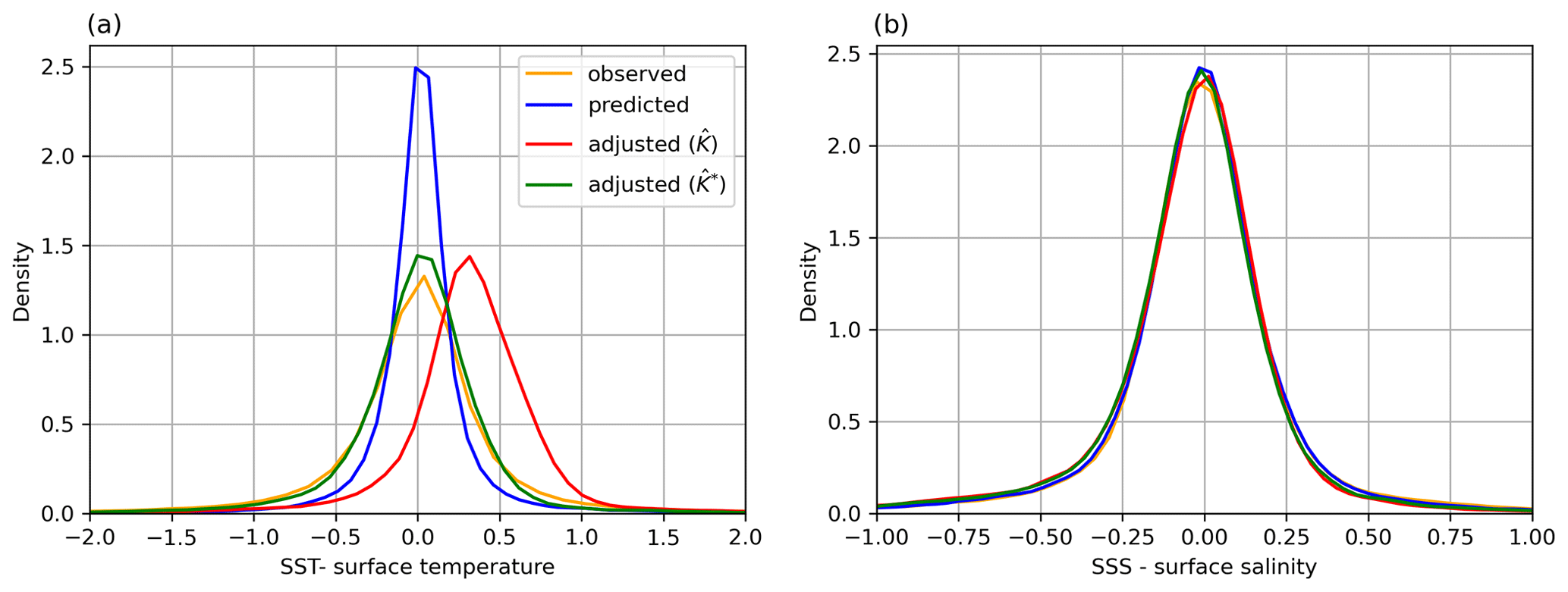
Figure 5Density distribution of the difference between the in situ surface temperature and salinity and the remote sensing SST and SSS. The predicted profiles (blue) correspond to the profiles produced by the NN alone. The adjusted distribution with is in red (also red in Fig. 4d). The adjusted distribution with is in green and corresponds to the OSnet product (i.e., NN + adjustment), also shown in green in Fig. 4d.
After computing the profiles, we reconstruct iteratively T−S profiles with the gradients multiplied by , starting from the bottom value (at z=1000 m) where (because the deepest MLD never reaches 1000 m, the maximum observed in the CORA dataset is H=628 m for our region). On a predicted temperature profile (the same is applied to salinity), the adjusted temperature profile is computed as follows:
and we retrieve the temperature profiles iteratively along depth by starting from the bottom m, where and :
Figure 5 presents the overall bias of surface and relative to SST and SSS. If we adjust gradients with a profile, the surface temperature is systematically too warm compared to SST (Fig. 5a, red). Now, if the adjustment is also increasing the gradients under the MLD (), the surface temperature bias is null (Fig. 5a, green). This supports our choice to amplify gradients just under the MLD () and to reduce them in the mixed layer (). Note that the direct prediction of temperature at the surface (Fig. 5a, blue) is more accurate compared to SST than in situ observations, because OSnet learns from SST. The salinity difference relative to SSS is too large for the adjustment to cause a significant issue (Fig. 5b). Still, the adjusted salinity profiles with K predicted create a fresh bias, and the use of corrects that.
A good example of profile prediction and adjustment is presented in Fig. 4. In this case the adjustment corrects perfectly the MLD estimate, from 30 m predicted (red) to 133 m adjusted (green). It reduces the T−S gradients above the MLD estimated from the K profile (K=0.5) and increases the T−S gradients just under this MLD. The decrease in T−S gradients in the mixed layer also removed the density inversion (Fig. 4c).
The adjustment proposed here reduces the variance of and above the MLD, reduces the number of density inversions, improves the predictions of the MLD (see Table 2) and increases the gradients in the transition layer under the MLD. For the adjusted profiles, the mean and standard deviation of gradients of σ0 over a 200 m-thick layer under the MLD are 1.38±0.9 kg m−3, which is closer to the observed values of than the predicted values of 1.24±0.8 kg m−3. The large summer gradients are especially well retrieved (not shown).
Table 2Metrics of accuracy for predictions of Armor3D, Glorys12, a neural network (NN, i.e., OSnet without MLD adjustment) and OSnet compared to the in situ CORA profiles. The σ0 inversions larger than 0.01 kg m−3 are counted. The Armor3D and Glorys12 statistics are computed on the subsampled products at the locations of the profiles of CORA.
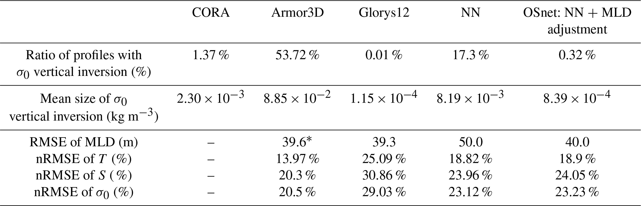
* All the MLDs are computed with the density criterion of 0.03, except for Armor3D, for which a different criterion is used to bypass their density inversion issues.
An alternative idea to solve the density inversion issue is to constrain the NN to predict profiles that are hydrostatically stable. The physical relationship can be implemented in the NN to enforce consistency on the predictions (Karpatne et al., 2017). This can be done by modifying the loss of the NN and penalizing the predictions with density inversions (Appendix A). This solution is elegant and allows us to predict directly profiles without density inversions. We provide this alternative approach here for the record of a negative result with regard to the design of such a NN. Indeed, profiles predicted with this custom loss still have poor MLD estimates compared to profiles and hence still need a posteriori adjustment. The modified loss (Appendix A) is not needed in this case because the MLD adjustment presented above happens to remove density inversions efficiently.
3.4 Explainability of the neural network
Explaining the predictive skills of the neural network is key to interpreting the prediction and strengthening trust in the model. It is also a useful tool in the development phase. Here, it gives insights into the relationship between surface data and in situ profiles. In this section, we use a game-theoretic approach to retrospectively estimate the relative importance of each input for each output. The algorithm, called SHapley Additive exPlanations (SHAP) (Lundberg and Lee, 2017), is a unified framework combining state-of-the-art methods to explain deep neural networks. It is based on a method called Deep Learning Important FeaTures (DeepLIFT) (Shrikumar et al., 2017) and Shapley values. DeepLIFT is a method for computing the effect of changing the original input to a reference value (uninformative background value for the input). The change in the output is representative of the importance of the input for predicting the output. Shapley regression values (Shapley et al., 1953) represent the impact of an input on the output by removing it from the input set and retraining this model with the subset of inputs. This being computationally expensive, it is possible to obtain an approximation of the effect of removing a variable from the model by integrating over samples from the training dataset using the Shapley sampling values (Štrumbelj and Kononenko, 2014). It produces an “importance” value for each particular prediction. The importance value is positive or negative, indicating the direction in which the input influences the output relative to the averaged output. The SHAP algorithm being computationally expensive, it was not possible to run it over the full dataset. After some tests, we found that 300 random samples were representative enough to obtain stable results for the average feature importance across the entire dataset.
4.1 Accuracy of the predictions compared to observations
Table 2 presents several metrics to evaluate OSnet, Armor3D and Glorys12 relative to CORA. Each dataset is predicted or subsampled at the locations of CORA profiles (in longitude, latitude, depth and time). The first two lines indicate the number and size of vertical density inversions. They indicate that the MLD adjustment of OSnet suppresses almost all density inversions, from 17.3 % to 0.32 % of profiles. Meanwhile, Armor3D has about 50 % of profiles with density inversions and Glorys12 almost none (0.01 %). Regarding the amplitude of density inversions, the MLD adjustment suppresses sufficiently large inversions and decreases by 1 order of magnitude the mean amplitude of inversions, from 10−3 to 10−4 kg m−3.
The root mean square error (RMSE) of the MLD (Table 2) indicates that the MLD adjustment improves the MLD RMSE of OSnet from 50 to 40 m, which is the same order of magnitude as Glorys12 (38.6 m) and Armor3D (39.4 m). Note that the MLD of Armor3D is computed with a different criterion to bypass density inversions. Armor3D uses the minimum of temperature and density threshold equivalent to a 0.2 ∘C decrease from the surface. The MLD of Armor3D computed with a density criterion of 0.03 kg m−3 yields a RMSE of 62.6 m. Finally, the global errors of temperature, salinity and density indicate that Armor3D profiles are the closest to the observed profiles. The metric is the normalized RMSE (nRMSE), which is the RMSE between predicted and observed profiles divided by the standard deviation of the observed profiles. It is a ratio of error compared to the variability observed. OSnet has a smaller nRMSE than Glorys12, and the MLD adjustment slightly increases the temperature nRMSE at the surface. Figure 3 reveals the vertical distribution of nRMSE. OSnet gives a more accurate prediction at the surface compared to both Armor3D and Glorys12, but Armor3D is closer to observations for the rest of the water column. Overall, the nRMSE of OSnet predictions is the same order of magnitude compared to other products, and it does not contain significant density inversions.
4.2 Temperature and salinity maps
Let us examine a daily map of temperature and salinity at ∘ resolution (Fig. 6). We chose a date in the pre-Argo era to illustrate the generalization skill of the OSnet product. All the maps reveal coherent horizontal structures. At the surface, the warm Gulf Stream detaches from Cape Hatteras and meanders further east, transforming into the North Atlantic Current (Fig. 6a, b). The surface confidence intervals are maximum for the cold and fresh waters near the edge of the continental slope and inside the cold and fresh core eddies and meanders (Fig. 6c, d). On average, confidence intervals highlight cold waters north of the Gulf Stream (Fig. 7a, b), which is consistent with the error of prediction maps presented in Buongiorno Nardelli (2020). This could be due to the lack of profiles containing these cold waters in our dataset. At depth (1000 m in Fig. 6e, f), the signature of large eddies is visible, associated with a maximum of the confidence interval again (Fig. 6g, h). The salty and warm Mediterranean Overflow Waters are seen in the southeast of the region. The average confidence interval at 1000 m is maximum along the Gulf Stream and its meanders, rather than in waters north of the Gulf Stream like at the surface (Fig. 7c, d). It corresponds to areas with the largest variability (Gaillard et al., 2016; Forget and Wunsch, 2007). Note the different color scale: the maximum confidence interval values at 1000 m depth are twice as small for temperature and 5 times smaller for salinity compared to the surface.
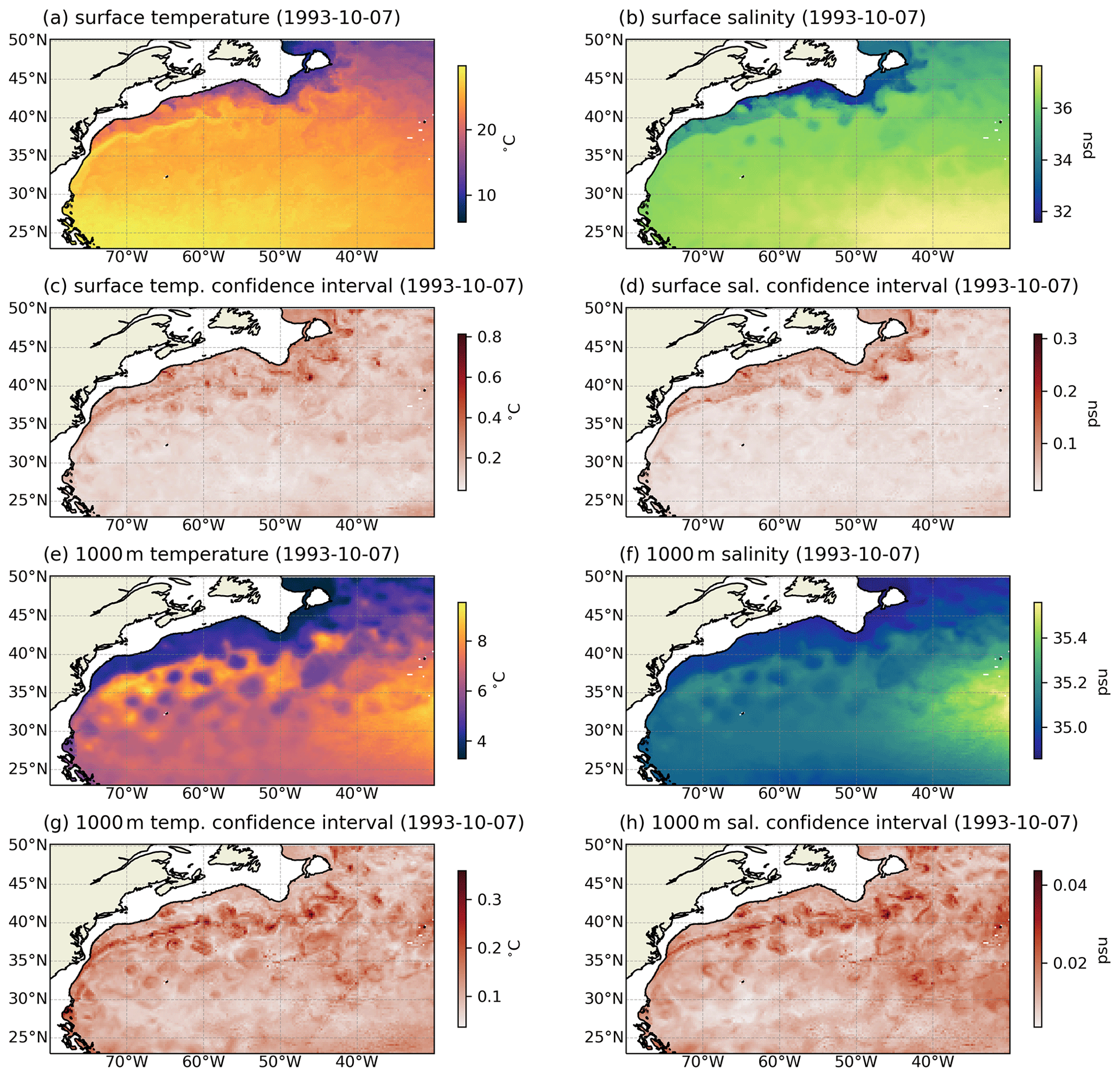
Figure 6OSnet temperature and salinity maps for 7 January 1993, at the surface (a, b) and at 1000 m (e, f). Their respective confidence intervals are displayed too, i.e., the standard deviation of the 15 bootstrapped models (c, d, g, h).
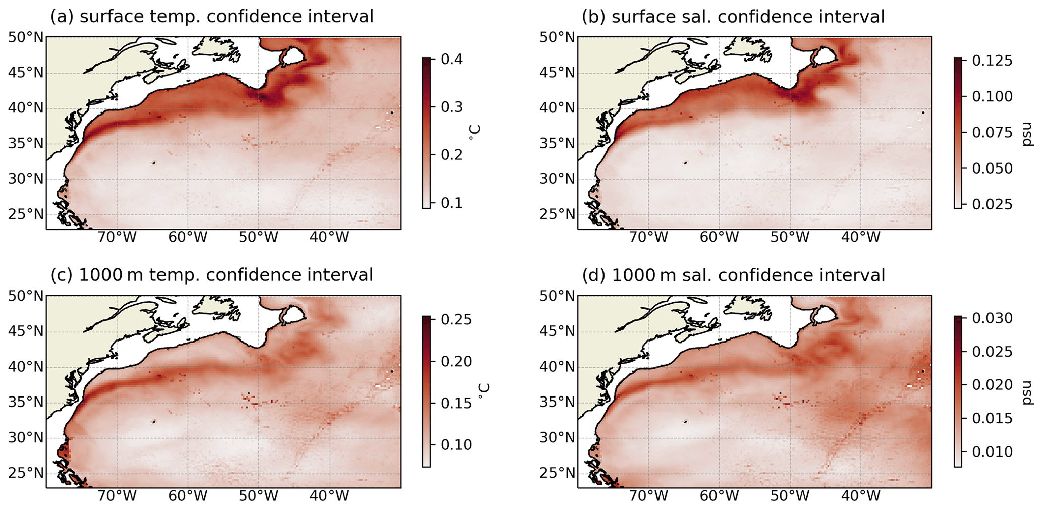
Figure 7Time average maps of the confidence intervals for surface and 1000 m temperature and salinity, i.e., the standard deviation of the 15 bootstrapped models.
4.3 MLD maps
To illustrate the quality of the predicted MLD of OSnet, we show MLD maps for a given day (5 January 2018) in Fig. 8. We picked a winter day to emphasize deep MLD areas. The direct prediction of the NN (Fig. 8a) has shallow patches in a few places that are due to density inversions. The density threshold is met too shallow due to these artifacts in the water column (see the profile example in Fig. 4). The MLD adjustment corrects these shallow patches, and the MLD field of OSnet looks more consistent and more similar to Glorys12. The OSnet MLD does not exhibit any very deep patch (MLD >300 m). These deep MLD events are rarely observed in CORA (1.7 % of the profiles have a MLD deeper than 300 m) but are often present in the MLD fields from Glorys12 (Fig. 8). They occur in warm meanders and eddies of the Gulf Stream. The MLD field of Armor3D (Fig. 8d) is for the week that contains 5 January 2018. It has several patches of either shallow or deep MLD (i.e., 28∘ N, 52∘ W or 48∘ N, 32∘ W) which look very sharp compared to OSnet and Glorys12. These patches might be regions around observed profiles for the given week, and the optimal interpolation of Armor3D is overfitting the profile at the expense of the general property field coherence. The Armor3D MLD is computed with a different criterion to bypass their density inversion issues. Still, some patches have no values where the criterion could not be matched (Fig. 8d).
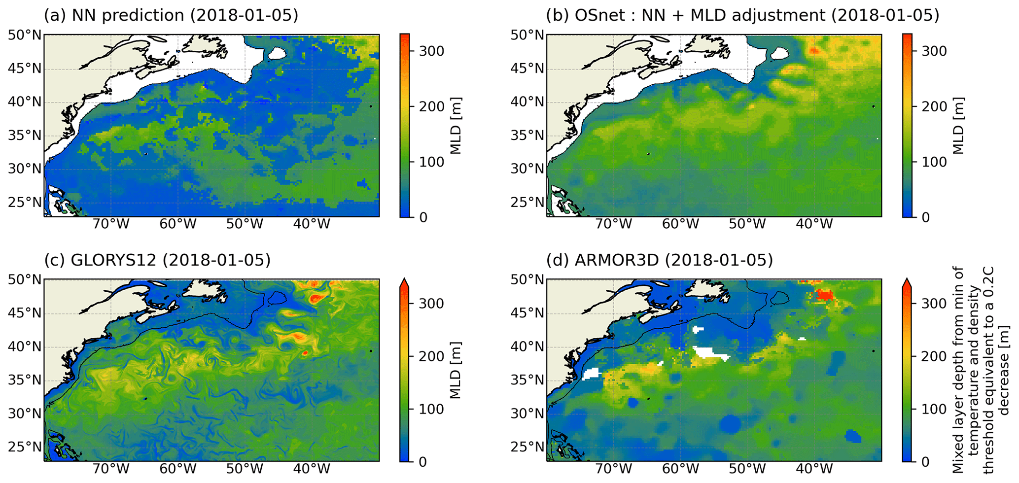
Figure 8MLD maps for 5 January 2018. Panel (a) shows the result of the NN alone (step 1 from the schematic Fig. 2) and panel (b) is the final OSnet product. Panels (c) and (d) are the MLDs of the TS profiles of Glorys12 and Armor3D. Armor3D is a weekly product, so the profiles here are for the first week of January 2018. All the MLDs are computed with the density criterion of 0.03, except for Armor3D, for which a different criterion is provided to bypass their density inversion issues. The shelf break is traced in black with the bathymetry contour of 1000 m. The maximum of the color bar is set by the maximum of OSnet.
Monthly MLD averages are presented for March and August in Fig. 9. The averages in 1∘ × 1∘ boxes for the in situ profiles (Fig. 9a, d) are compared to OSnet (b, e) and Glorys12 (c, f). The three estimates are in good agreement with each others and with climatologies not shown here (Holte et al., 2017; Sallée et al., 2021). The main structures are well respected with a large winter patch of deeper MLD extending between the Gulf Stream and the subtropical gyre. In winter, vigorous air–sea fluxes extract heat from the ocean and erode the superficial stratification. This process activates convective mixing and deepens the mixed layer, ventilating and creating the Eighteen Degree Mode Water (Speer and Forget, 2013; Maze and Marshall, 2011). In summer the near-surface water warms and caps the mode water layer. The summer MLD is shallower everywhere with a slightly deeper signature in the core of the Gulf Stream, as it separates from the coast at Cape Hatteras. A deeper summer MLD is also found south of ∼30∘ N along the equatorward edge of the subtropical gyre (Fig. 9d, e, f), a feature also observed in the climatology of de Boyer Montegut et al. (2004). This tropical summer MLD deeper than 30 m is marked by the trade winds (Stramma and Schott, 1999). The large permanent anticyclonic “Mann eddy” (Mann, 1967; Rossby, 1996) is clearly visible as a deep mixed-layer patch at 43∘ N, 42∘ W (Fig. 9). A region of the deeper MLD is also visible along the North Atlantic Current, deeper in OSnet than in Glorys12.
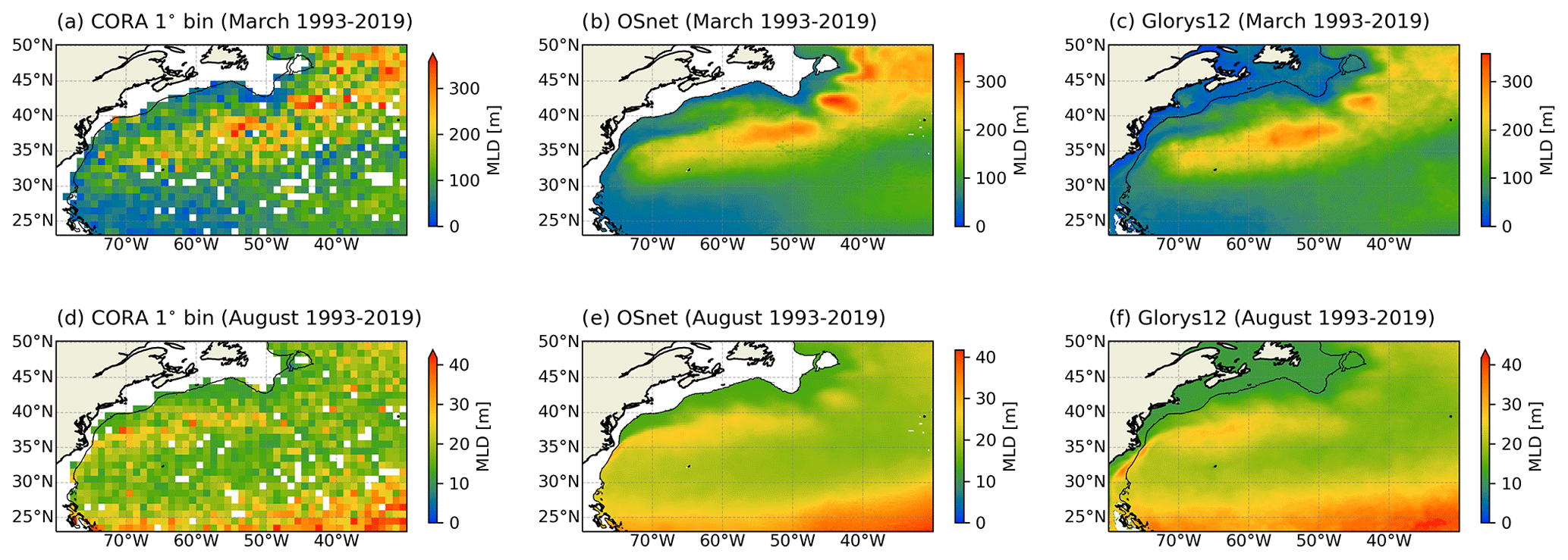
Figure 9Maps of the monthly mean of the MLD defined with a density threshold of 0.03 kg m−3 for (a, d) CORA T−S profiles averaged by bins of 1∘ (b, e) OSnet and (c, f) Glorys12. The months of March and August are representative of the seasonal range of the MLD for the region. Note the different color-bar range for each month. The maximum of the color bar is set by the maximum of OSnet. The shelf break is traced in black with the bathymetry contour of 1000 m.
4.4 Importance of each input for the reconstruction
In Figs. 10 and 11 we present the absolute values of the relative importance of each input, on each output, averaged over depth, over the 300 test profiles and over the 15 bootstrapped models. Error bars correspond to the standard deviation of the 15 models. To be comparable, the importance values of the inputs are normalized so that the sum per output is equal to 1. Figures 10 and 11 give a general overview of what the NN uses for the predictions. These importance values can also be displayed for a specific profile or by depth levels, seasons, or geographical regions, providing insights to elucidate the behavior of the NN. The main result here is that SST is the main driver for estimating T, S and MLD profiles (Fig. 10). As expected, it is especially important for predicting surface temperature. MDT is the second-most important variable, and it is the most important deeper than ∼200 m (Fig. 11). The latitude, longitude, SLA and day of the year equally concur to explain the predictions. The rest of the input variables, i.e., bathymetry and the surface geostrophic currents derived from SLA, are smaller contributions to the predictions. Even if they have small contributions on average, they can be important for a specific profile. The cosine of the day of the year is very important for the prediction of the MLD (Fig. 10), probably because it is in phase with the MLD seasonal cycle, while temperature and salinity cycles are in phase with the sine of the days (not shown). Still, it means that the day of the year alone drives ∼29 % of the MLD predictions, which is equivalent to the importance of SST for MLD predictions (∼29 % too).
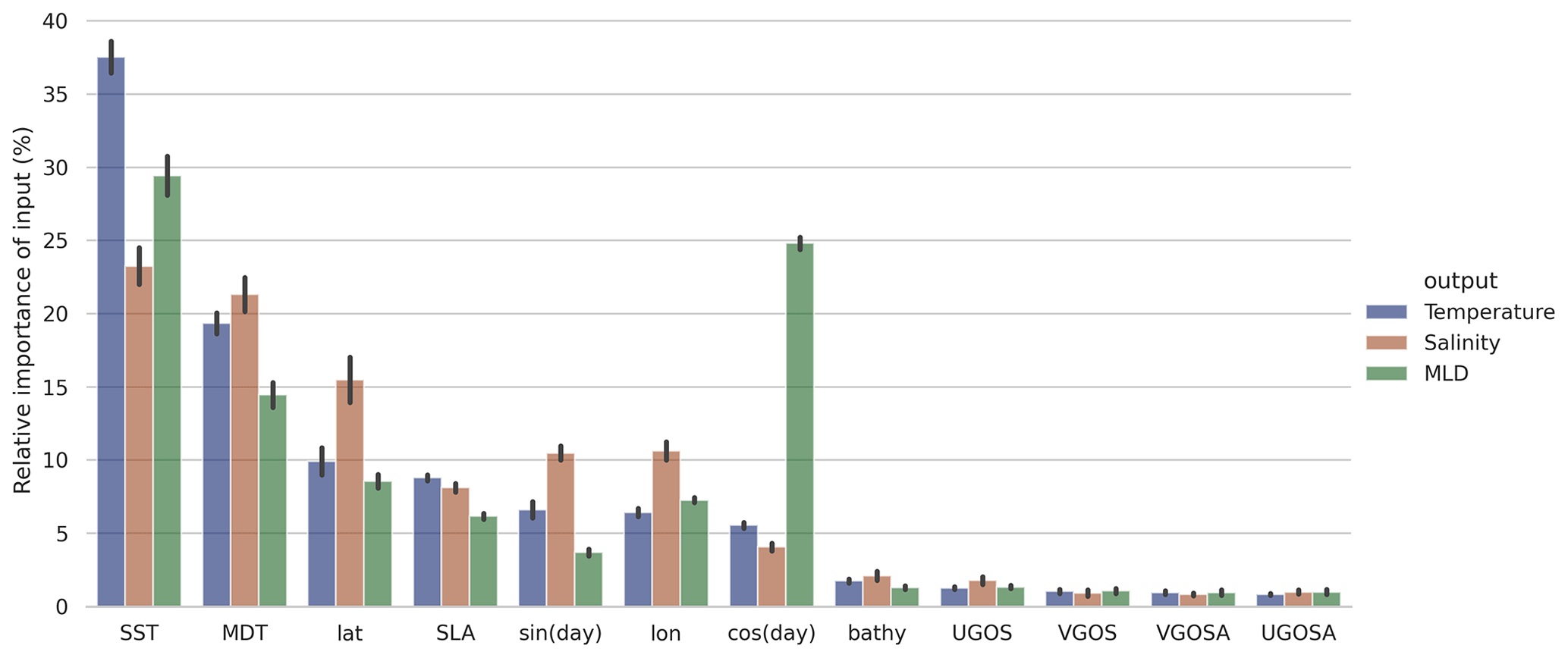
Figure 10Relative importance of each input for each output, averaged by depth. The inputs (x axis) are sorted by importance for the temperature to have the largest importance on the left of the plot. The cosine of the day of the year is more important than the sine for the MLD prediction because the cosine is in phase with the seasonal cycle of the MLD.
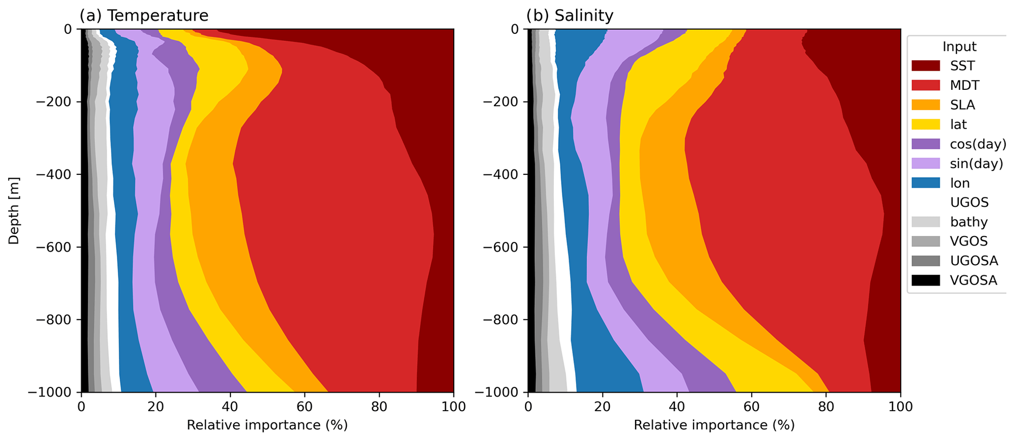
Figure 11Relative importance of each input for each output, averaged by depth. The areas are sorted by variance to have the input with the largest difference of impact by depth to the right of each panel.
4.5 Time series of surface properties
To assess the accuracy of OSnet through time, we analyze the time series of the spatially averaged surface temperature and compare it to the observed SST time series as well as the Glorys12 and Armor3D products. We average data over the region after removing values on the shelf (bathymetry >1000 m). The long-term trends are obtained by applying a seasonal-trend decomposition based on local regression (STL) (Cleveland et al., 1990). STL is a filtering procedure that extracts three components: (i) the variations in the data at the seasonal frequency (Fig. 13), (ii) the low-frequency variation together with nonstationary and long-term changes (Fig. 12) and (iii) a remaining high-frequency component.
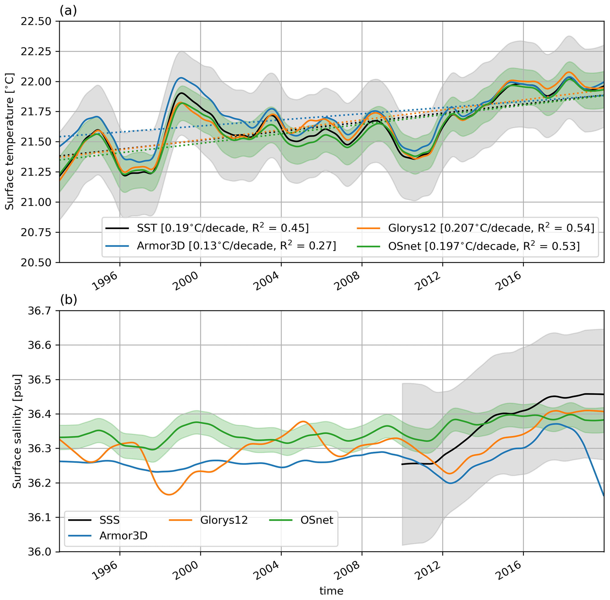
Figure 12Nonseasonal low-frequency time series of surface temperature (a) and salinity (b) averaged over the region excluding the shelf shallower than 1000 m. It is extracted with a seasonal-trend decomposition. The linear trends of temperature are displayed with dashed lines, and their slope and R2 are in the legend of panel (a). The grey shaded areas are the SST mapping error in (a) and the SSS random error (b). The green shaded areas are the OSnet confidence intervals, i.e., the standard deviation of the 15 bootstrapped models.
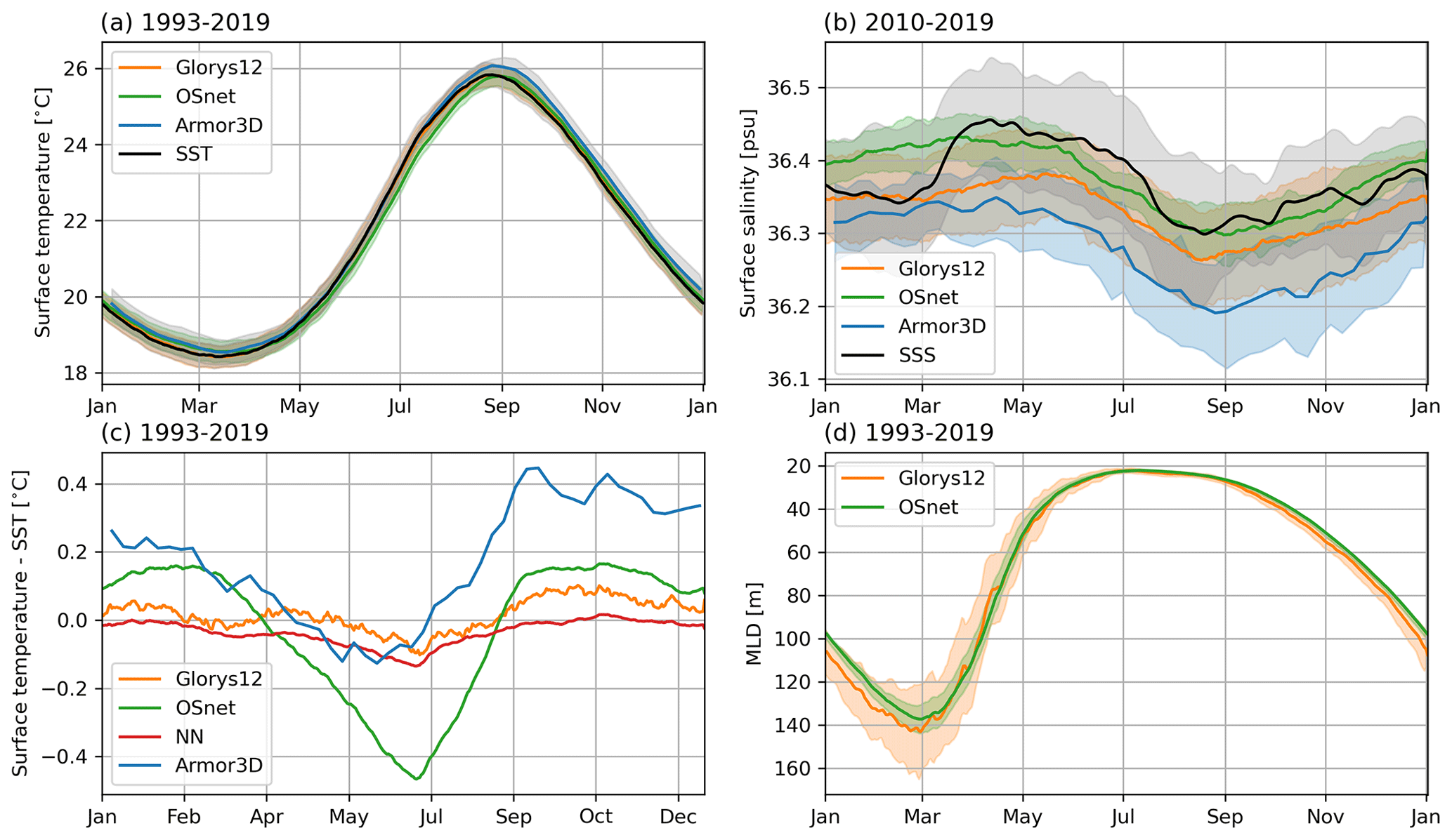
Figure 13Seasonal variation of the mean surface temperature (a), surface salinity (b) and MLD (d) for OSnet, Armor3D and Glorys12 compared to remote sensing SST and SSS (black). The difference between SST and the surface temperature is displayed in panel (c), with the direct prediction of the NN hence without MLD adjustment in red. It is averaged over the period 1993–2019 excluding the shelf shallower than 1000 m, except for the surface salinity because SSS only ranges from 2010 to 2019. The bands or errors are the standard deviation over the time period.
OSnet follows best the long-term trend of SST with a linear trend of 0.197 ∘C/decade, close to the SST trend of 0.190 ∘C/decade (Fig. 12a). For comparison, the surface-averaged temperature of Armor3D is warmer in the pre-Argo years, probably due to their background global average that is mostly composed of Argo floats. This is a validation that OSnet generalizes well and is not biased towards the recent years of in situ observations. Regarding surface salinity long-term trends, no significant trend is captured over the 1993–2019 period (Fig. 12b). There is no clear agreement between the different datasets, except in the last period, 2010 to 2019, where all averages increase like the SSS signal. Armor3D mean surface salinity drops significantly during the last 2 years, 2018 and 2019, out of the SSS error margin. Note that OSnet does not include the areas over the continental shelf and does not predict deeper than 1000 m. A significant part of the climatic signal takes place in the coastal regions (Ezer et al., 2013; Davis et al., 2017), and an improvement of OSnet would be to deal with profiles of different lengths in order to include these regions.
The mean seasonal variation of surface temperature, salinity and MLD is presented in Fig. 13. We compute it by averaging the signal by day of the year (week of the year for Armor3D). The surface temperature seasonal signal is well reproduced for each dataset, as expected considering that SST is included in the input of OSnet and used to produce both Armor3D and Glorys12 (Fig. 13a). A close observation of the curves in Fig. 13a shows that the seasonal cycle of OSnet surface temperature is too cold between May and September (Fig. 13c). This is due to the MLD adjustment, since the direct prediction of surface temperature gives a very precise seasonal cycle of SST (red line in Fig. 13c). Armor3D seasonal temperature is warmer from August to April, which could be a bias caused by the undersampling of the pre-Argo, colder years (Fig. 13c). This bias is also present in the temperature time series (Fig. 12a).
The surface salinity seasonal signal is noisier, in part because it presents inter-annual variations that are the same order of magnitude as the seasonal variations (Fig. 13b). We compare 2010–2019 because it is the only period available for the SSS product. OSnet surface salinity is the closest to SSS compared to the predictions of Armor3D and Glorys12, which are both fresher than the observed SSS. We observe a delay in the SSS seasonal variations: it is fresher by almost 0.1 psu from January to March. We discuss this in Appendix B and Fig. A1.
Finally, the seasonal cycle of MLD (Fig. 13d) in the region is asymmetrical, with slow deepening from summer to winter and fast shoaling during the early spring. This asymmetry is expected since buoyancy loss at the surface leads to convective mixing (hence deepening the mixed layer requires buoyancy loss over an ever-increasing water column depth), while buoyancy gain directly leads to a stable stratification and shallow mixed layer (e.g., Taylor and Ferrari, 2010). OSnet MLD compares well to the MLD computed on Glorys12. We do not present the MLD of Armor3D here because it is computed with a different criterion. The winter MLD variance is larger in Glorys than OSnet, which is also observed on daily maps of MLD. Events of deep MLDs are not represented in OSnet (Fig. 8).
In the results section we have seen that OSnet predictions are overall coherent. We now want to assess whether OSnet can be used to help interpret local oceanographic measurements or for process studies. The goal is to be as close as possible from observations while being physically consistent. To do so, OSnet is compared to observations (remote and in situ) and to the other two products, Armor3D and Glorys12. In this section we present these comparisons and discuss the quality of our predictions.
5.1 Comparison to observed data
One major feature of OSnet is the possibility of estimating T and S profiles at any location, given that surface data are available. Here we predict T−S at the location of a mooring of the line W (Fig. 14) and along the hydrographic section AT20 (Fig. 15). Temperature and salinity at 1000 m are plotted in comparison to mooring data for a period of 3 years (10 May 2004 to 11 March 2007). OSnet corresponds well to observations but with a slight warm and fresh shift in the first year (Fig. 14). A warm-core eddy crosses the location of the mooring in 2006 (see the SLA map in Fig. 14a), and its warm and salty deep signature is well captured by OSnet. Smaller warm and salty spikes appear in October 2004 and July and November 2005 but are not visible in the mooring data. They correspond to warm meanders of the Gulf Stream revealed by the SST and SLA at these three periods (not shown), causing deep T−S changes in OSnet.
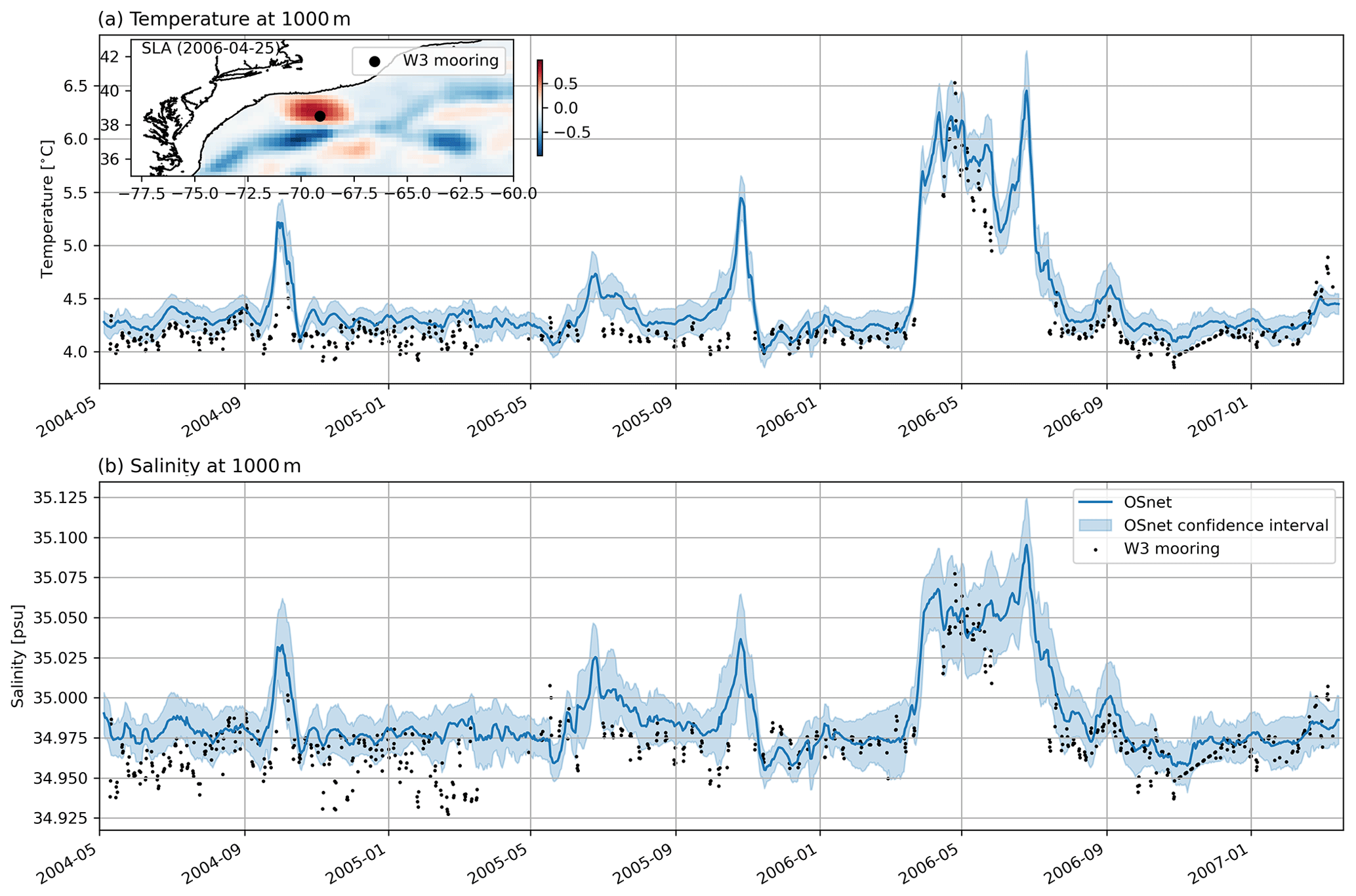
Figure 14OSnet prediction of temperature and salinity at 1000 m (blue) at the location of a mooring of line W3 (black, 69.11∘ W, 38.51∘ N). The map of SLA in the temperature panel is for 25 April 2006, when a warm-core eddy went through the mooring location. These mooring data are not included in the learning dataset of OSnet.
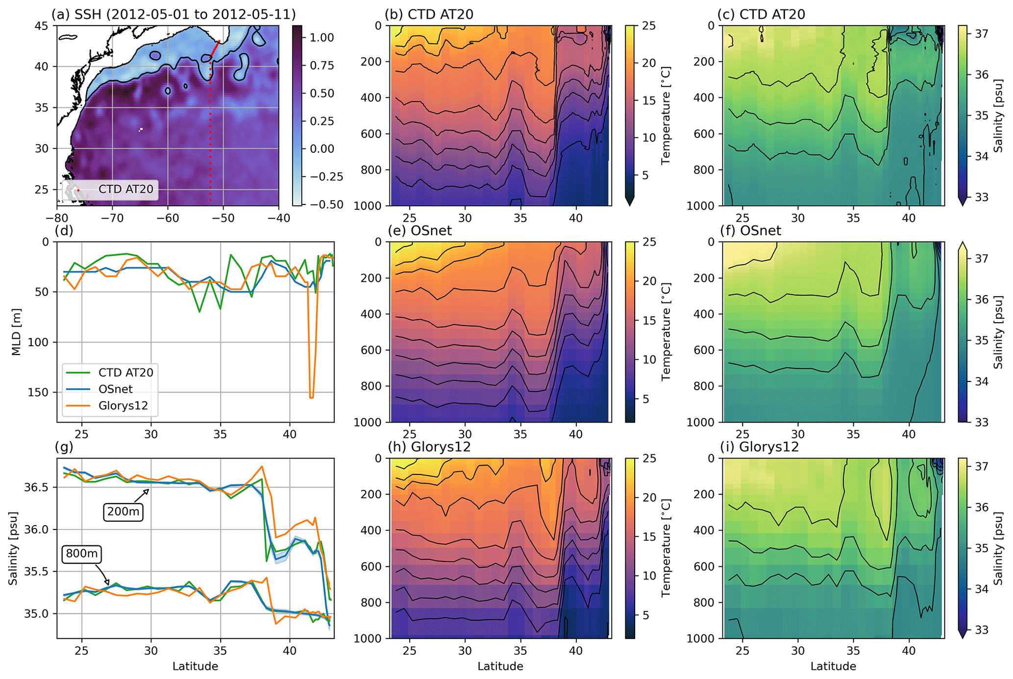
Figure 15Hydrographic section AT20 (a, b, c) sampled along the 52.3∘W meridian by the research vessel Atlantis from 1 to 5 May 2012. Temperature and salinity profiles are estimated with OSnet (e, f) at the exact locations of the sampled CTDs by interpolating the input data at those locations. Glorys12 profiles (h, i) are collocated in time and space with the CTD profiles. The SSH in panel (a) is averaged over the sampling period of the section. The MLDs in panel (d) are computed with the density threshold of 0.03. Salinity segments at 200 and 800 m are plotted along latitude in panel (g) with confidence intervals in blue bands around the mean value for OSnet, i.e., the standard deviation of the 15 bootstrapped models. The contour intervals for the plot section are 0.5 psu from 33 to 37 psu for salinity and 2 ∘C from 4 to 24 ∘C for temperature.
We compare the OSnet T−S structure along the hydrographic section AT20 sampled in May 2012 by the research vessel Atlantis (Fig. 15). The OSnet prediction is done at the exact locations of the conductivity–temperature–depth (CTD) profiles, interpolated linearly on the maps of input data (Table 1). The comparison is also done for Glorys12 but by collocating the profiles with a nearest neighbor method. Both Glorys12 and OSnet predictions are coherent, but we note two specific biases in Glorys12. First, Glorys12 displays a deep patch of MLD around 41∘ N, north of the Gulf Stream, that is not observed by the CTDs nor predicted by OSnet (Fig. 15d). This deep MLD could be due to the nearest neighbor selection of the profile that is not exact in the case of Glorys12, or it could be an artifact of their model. Indeed, deep patches of MLD are also visible on daily MLD maps of Glorys12 but are absent on the OSnet daily MLD maps (Fig. 8). Second, the salinity reconstruction of Glorys12 differs more from the observed data north of the Gulf Stream (Fig. 15g). OSnet performs very well along this section in comparison to Glorys12.
5.2 OSnet to explore theoretical inputs
Since OSnet is very easy and fast to manipulate to make predictions, it can be used to make predictions using theoretical inputs. To illustrate this, we seek the interior signature of eddies detected with altimetry. We make two predictions of temperature and salinity for a section across two particular eddies observed on 6 October 2006 (Fig. 16a): one prediction is based on all observational inputs (Fig. 16b, c), and the second prediction is made by removing the eddy signature in SLA; we simply set it to 0 (Fig. 16e, f, g). The interior temperature and salinity anomalies associated with the eddies are obtained by difference (Fig. 16h, i). Anomalies are the largest at depth around m with amplitudes of a few degrees per meter of SLA. These are reasonable amplitudes and structures for the region (Castelao, 2014) and illustrate how OSnet could easily be used to extract more knowledge than the standard realistic T−S predictions on a grid.
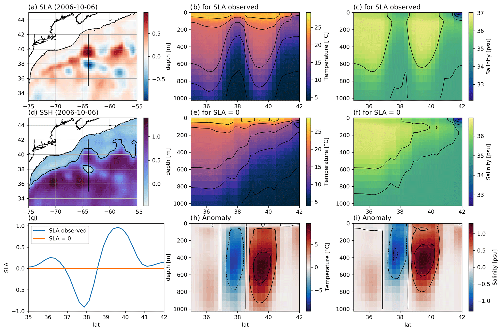
Figure 16Prediction of T−S profiles for a section across two meanders of the Gulf Stream (b, c) and for a simulated SLA flattened to zero (e, f). The meanders are visualized with maps of SLA (a) and SSH d, which are computed by adding MDT and SLA for 6 October 2006. The anomaly between the T−S sections for the observed SLA and the simulated SLA is displayed in panels (h) and (i). The SSH contour in panel (d) is 0.1 m to represent the Gulf Stream.
5.3 Potential improvement of the method
Several improvements of the method could be made in the future. One important limitation is the current NN architecture that prevents predictions of profiles of different lengths. It constrains the analysis to use a fixed maximum depth and thus prevents profiles from being kept shorter than that maximum depth. A solution would be to develop a custom loss that can deal with empty variables. Another way would be to add depth as an input variable like in Buongiorno Nardelli (2020). In that case, we could predict properties over shallow bathymetry and also deeper than our rather arbitrary 1000 m limit.
OSnet produces coherent horizontal and temporal patterns even though each profile is predicted independently. Yet we wonder how using horizontal and temporal surface gradients as inputs could improve predictions, especially in frontal regions. To test this, we would need to work with three-dimensional (long–lat–time) patches of input data for each profile location and to build a different NN architecture (e.g., Ouala et al., 2018; Jouini et al., 2013; Tandeo et al., 2013; Lguensat et al., 2018) that takes patches of data as input and profiles as output. Convolutional neural architectures accounting for irregularly sampled space–time observations might also be appealing (Fablet et al., 2021). The expected result would be sharper fronts, as we observe that fronts from OSnet are smoother than in observations, e.g., Fig. 15. We wonder whether the NN could learn from the temporal surface gradient to anticipate vertical changes in stratification.
Prediction intervals (PIs), also called “coverage probability”, could be computed as a complement of confidence intervals (Khosravi et al., 2011). While the confidence intervals (Fig. 7) give the range of variation of a set of NNs with different initializations and training datasets, the PI gives the probability of the observation associated with the prediction being in a range of values. The PI can be obtained by adding output variables to the proposed architecture. Here, the PI could be represented as temperature and salinity profiles around the prediction, representing the 95 % interval. It means there would be a 95 % probability of the true value associated with the prediction lying within the interval.
Given the very promising results of our study, obvious future work would be to apply OSnet in other more challenging regions, with fewer data or more complicated vertical structures and different dynamics. Also, the 3D geostrophic velocities of the OSnet gridded product could be estimated using the thermal wind equation combined with surface altimeter geostrophic currents (Mulet et al., 2012). Finally, since we found that OSnet correctly captures the SST warming trend (Fig. 12a) and mesoscale structures, it would be interesting to apply OSnet to other boundary currents and to compare the resulting OHC estimates to previous reconstructions (e.g., Cheng et al., 2017). Other global ocean indicators such as ocean freshwater content or steric sea level could be investigated as well.
We proposed a method to estimate the ocean stratification from surface data using a neural network trained from in situ historical data. The originality of this study is the attention we gave to the vertical coherence of T−S profiles, in particular the accuracy of MLD predictions and the absence of unrealistic vertical density inversions. The global nRMSEs of T and S are better than a state-of-the-art ocean re-analysis (Glorys12) but worse than Armor3D predictions. However, OSnet predictions do not have any unrealistic density inversions, while Armor3D does. Each OSnet profile is predicted independently, but OSnet produces coherent horizontal patterns on a ∘ daily grid, especially for MLD. In addition, the pre-Argo years are well reconstructed, which supports the good generalization skill of OSnet. Confidence intervals issued from the bootstrapped method provide an estimate of the prediction variability. Confidence is lower in the cold surface waters north of the Gulf Stream and in the jet at depth, which corresponds to the most variable areas. The reconstructed surface temperature reproduces the observed warming trend. The seasonal cycle of surface salinity matches best the one of SSS compared to Glorys12 and Armor3D.
One convenient feature of OSnet is the possibility of estimating profiles at any location, given that the surface data are provided. This allows us to compare predicted profiles at the exact location of the observed CTD, for example. It is computationally inexpensive to run, and we encourage anyone who needs to predict ocean stratification from surface data to use OSnet. Another feature is the possibility of computing the relative importance of each input for each T−S prediction and analyzing which surface features influence most which properties. This is a development tool that can also be used to study how the ocean stratification reflects on the surface data. Finally, the horizontal resolution of OSnet is constrained at ∘ by the resolution of the SLA. The upcoming satellite mission SWOT should provide higher-resolution observations for OSnet to learn and predict smaller-scale features.
A1 Custom loss function
Without constraining the predictions in a physical space, most profiles show spurious density inversions that make the MLD computation impossible. To alleviate these issues, we develop a custom loss that constrains the density profile to be monotonous and the properties in the mixed layer to be well mixed. The loss function is the minimization of the mean square error between our prediction and the target profiles, which we complement with a physics-constrained loss LossPhy and LossH:
with N the batch size and the predicted and y the observed profiles of temperature and salinity as tensors of size (D=51 depth levels). To that standard loss we add two more terms. First we include the potential density σ0 profile in the target y and prediction . It ensures that the T−S predictions correspond to a profile of density closer to the observed density profile. We also take the profile K out of the standard loss and multiply by a coefficient λMLD:
Second, we add a constraint of monotony on the density profile to penalize the predictions that contain density inversions. A positive value of Δσ0 is a violation of the hydrostatic stability of the water column. Such density inversion can exist in observed profiles at small temporal and vertical scales. As our predicted profiles are daily averages, we assume that they should not present any density inversions, i.e., Δσ0<0, strictly.
A2 Optimization of the λ coefficient
The λ coefficient of our custom loss needs to be optimized in order to minimize three metrics. A metric of accuracy is the root mean square error of the target relative to the prediction,
and two metrics of physical consistency, the root mean square error of the MLD H,
and m3 the count of density inversions. Note that the in m2 is directly predicted by the NN; it is not computed on the predicted profiles with the density criterion. This is a multi-objective problem that we solve with the NSGA-II genetic algorithm (Deb et al., 2002).
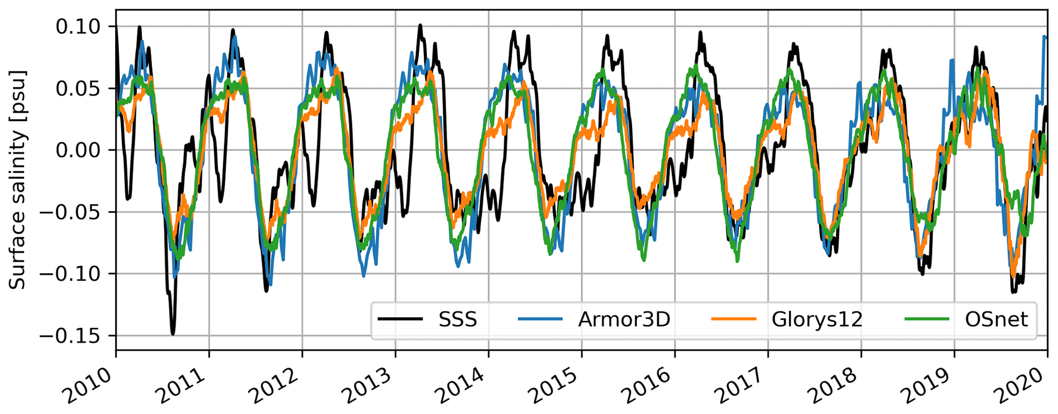
Figure A1Periodic signal of the mean surface salinity from OSnet (green), Glorys12 (orange), Armor3D (blue) and remote sensing (black). The periodic signal is extracted using an STL decomposition. The SSS seasonal variation is delayed each year in winter until the 2017–2018 winter.
We observe a delay in the SSS seasonal variation. It is fresher by almost 0.1 psu from January to March (Fig. 13b). The periodic signal of SSS is different from 2010 to 2017 compared to the other three products but seems corrected for the 2018 and 2019 winters (Fig. A1). The authors of the SSS-CCI dataset (Boutin et al., 2021) also noticed larger seasonal biases in the SSS with respect to Argo salinities before mid-2015 over the global ocean. The largest differences relevant for our region are observed in high-latitude cold waters and boreal winter above 47∘ N. After 2015 the integration of a new satellite (SMAP) and a change in the calibration mode of the satellite used over the period 2010–2019 (SMOS) in November 2014 improved the quality of the seasonal signal (Boutin et al., 2021).
The complete code to process input data and to develop a fully trained OSnet model is available at https://github.com/euroargodev/OSnet (Pauthenet et al., 2022b). A simpler version, focusing on making predictions with OSnet, is also available at https://github.com/euroargodev/OSnet-GulfStream (Pauthenet et al., 2022c). The OSnet gridded temperature and salinity daily fields of the 0–1000 m Gulf Stream region from 1993 to 2019 are available at https://doi.org/10.5281/zenodo.6011144 (Pauthenet et al., 2022a).
The CORA hydrographic profiles are available at https://www.seanoe.org/data/00351/46219/ (last access: 27 June 2022, Szekely et al., 2022). MDT CNES-CLS2018 is available at https://www.aviso.altimetry.fr/en/data/products/auxiliary-products/mdt/mdt-global-cnes-cls18.html (last access: 27 June 2022, Mulet et al., 2022b). The SST dataset is available at https://doi.org/10.5285/62c0f97b1eac4e0197a674870afe1ee6 (Good et al., 2019). SLA and derived variables are available through the CMEMS portal at https://www.copernicus.eu/en/access-data/copernicus-services-catalogue/global-ocean-gridded-l4-sea-surface-heights-and-derived (last access: 27 June 2022, CMEMS, 2022). The SSS CCI dataset is available at https://catalogue.ceda.ac.uk/uuid/4ce685bff631459fb2a30faa699f3fc5 (last access: 27 June 2022, Boutin et al., 2022). Armor3D is available through the CMEMS portal at https://doi.org/10.48670/moi-00052 (Mulet, 2022a). Glorys12 is available through the CMEMS portal at https://doi.org/10.48670/moi-00021 (Drévillon et al., 2022). Bathymetry ETOPO1 can be found at https://www.ngdc.noaa.gov/mgg/global/ (last access: 27 June 2022, NOAA, 2009). The Line W mooring data are available at https://scienceweb.whoi.edu/linew/ (last access: 27 June 2022, Toole et al., 2022). The hydrographic section AT20 is accessible at https://cchdo.ucsd.edu/cruise/33AT20120419 (McCartney, 2012).
GM proposed the project of using NN to predict T−S profiles and did preliminary analyses. LB and EP developed the Python codes, and GM tested it and wrapped it in a user-friendly package. LB, PT and RF brought expert advice on neural networks, KB eased the access to datasets and helped with the general workflow, and AMT, FR and GM provided ideas for the development of the method and the oceanographic pertinence of the study. EP wrote the paper, and all the coauthors contributed.
The contact author has declared that none of the authors has any competing interests.
Publisher’s note: Copernicus Publications remains neutral with regard to jurisdictional claims in published maps and institutional affiliations.
Etienne Pauthenet is funded by the Euro-Argo RISE project of the European Union's Horizon 2020 research and innovation programme (grant no. 824131). Anne-Marie Tréguier is supported by CNRS and by the MEDLEY project, funded by JPI Climate and JPI Oceans under the 2019 joint call. Etienne Pauthenet would like to thank Tanguy Szekely, Camille Lique, Claude Talandier and Alexandre Supply for the useful discussions around the study and Sean Tokunaga for his inspiring preliminary work on this subject.
This research has been supported by Euro-Argo RISE project of the European Union’s Horizon 2020 research and innovation programme (grant no. 824131).
This paper was edited by Anna Rubio and reviewed by Michel Crepon and one anonymous referee.
Abadi, M., Barham, P., Chen, J., Chen, Z., Davis, A., Dean, J., Devin, M., Ghemawat, S., Irving, G., and Isard, M.: Tensorflow: A system for large-scale machine learning, in: 12th {USENIX} symposium on operating systems design and implementation ({OSDI} 16), Savannah, GA, USA, 2–4 November 2016, 265–283, ISBN 978-1-931971-33-1, 2016. a
Argo: Argo float data and metadata from Global Data Assembly Centre (Argo GDAC), SEANOE [data set], https://doi.org/10.17882/42182, 2022. a
Boutin, J., Reul, N., Köhler, J., Martin, A., Catany, R., Guimbard, S., Rouffi, F., Vergely, J.-L., Arias, M., and Chakroun, M.: Satellite‐Based Sea Surface Salinity Designed for Ocean and Climate Studies, J. Geophys. Res.-Oceans, 126, e2021JC017676, https://doi.org/10.1029/2021JC017676, 2021. a, b, c, d, e
Boutin, J., Vergely, J.-L., Reul, N., Catany, R., Koehler, J., Martin, A., Rouffi, F., Arias, M., Chakroun, M., Corato, G., Estella-Perez, V., Guimbard, S., Hasson, A., Josey, S., Khvorostyanov, D., Kolodziejczyk, N., Mignot, J., Olivier, L., Reverdin, G., Stammer, D., Supply, A., Thouvenin-Masson, C., Turiel, A., Vialard, J., Cipollini, P., and Donlon, C.: ESA Sea Surface Salinity Climate Change Initiative (Sea_Surface_Salinity_cci): weekly and monthly sea surface salinity products, v2.31, for 2010 to 2019, Centre for Environmental Data Analysis, [data set], https://doi.org/10.5285/4ce685bff631459fb2a30faa699f3fc5, last access: 27 June 2022. a
Breiman, L.: Bagging predictors, Mach. Learn., 24, 123–140, https://doi.org/10.1007/BF00058655, 1996. a
Buongiorno Nardelli, B.: A Deep Learning Network to Retrieve Ocean Hydrographic Profiles from Combined Satellite and In Situ Measurements, Remote Sens., 12, 3151, https://doi.org/10.3390/rs12193151, 2020. a, b, c, d
Buongiorno-Nardelli, B. and Santoleri, R.: Methods for the reconstruction of vertical profiles from surface data: Multivariate analyses, residual GEM, and variable temporal signals in the North Pacific Ocean, J. Atmos. Ocean. Tech., 22, 1762–1781, 2005. a
Cabanes, C., Grouazel, A., von Schuckmann, K., Hamon, M., Turpin, V., Coatanoan, C., Paris, F., Guinehut, S., Boone, C., Ferry, N., de Boyer Montégut, C., Carval, T., Reverdin, G., Pouliquen, S., and Le Traon, P.-Y.: The CORA dataset: validation and diagnostics of in-situ ocean temperature and salinity measurements, Ocean Sci., 9, 1–18, https://doi.org/10.5194/os-9-1-2013, 2013. a
Castelao, R. M.: Mesoscale eddies in the South Atlantic Bight and the Gulf Stream recirculation region: vertical structure, J. Geophy. Res.-Oceans, 119, 2048–2065, 2014. a
Charantonis, A. A., Badran, F., and Thiria, S.: Retrieving the evolution of vertical profiles of Chlorophyll-a from satellite observations using Hidden Markov Models and Self-Organizing Topological Maps, Remote Sens. Environ., 163, 229–239, 2015. a
Cheng, L., Trenberth, K. E., Fasullo, J., Boyer, T., Abraham, J., and Zhu, J.: Improved estimates of ocean heat content from 1960 to 2015, Sci. Adv., 3, e1601545, https://doi.org/10.1126/sciadv.1601545, 2017. a
Chollet, F. and Others: Keras, https://github.com/fchollet/keras (last access: 27 June 2022), 2015. a
Cleveland, R. B., Cleveland, W. S., McRae, J. E., and Terpenning, I.: STL: A seasonal-trend decomposition, J. Off. Stat., 6, 3–73, 1990. a
CMEMS: Global ocean gridded l4 sea surface heights and derived, [data set], https://www.copernicus.eu/en/access-data/copernicus-services-catalogue/global-ocean-gridded-l4-sea-surface-heights-and-derived, last access: 27 June 2022. a
Contractor, S. and Roughan, M.: Efficacy of Feedforward and LSTM Neural Networks at Predicting and Gap Filling Coastal Ocean Timeseries: Oxygen, Nutrients, and Temperature, Front. Mar. Sci., p. 368, https://doi.org/10.3389/fmars.2021.637759, 2021. a
Davis, X. J., Joyce, T. M., and Kwon, Y.-O.: Prediction of silver hake distribution on the Northeast US shelf based on the Gulf Stream path index, Cont. Shelf Res., 138, 51–64, 2017. a
de Boyer Montegut, C., Madec, G., Fischer, A. S., Lazar, A., and Iudicone, D.: Mixed layer depth over the global ocean: An examination of profile data and a profile based climatology, J. Geophys. Res.-Oceans, 109, 1978–2012 2004. a, b
Deb, K., Pratap, A., Agarwal, S., and Meyarivan, T.: A fast and elitist multiobjective genetic algorithm: NSGA-II, IEEE T. Evolut. Comput., 6, 182–197, 2002. a
Drévillon, M., Fernandez, E., and Lellouche, J. M.: Glorys global ocean physics reanalysis GLOBAL_MULTIYEAR_PHY_001_030, [data set], https://doi.org/10.48670/moi-00021, last access: 27 June 2022. a
Durack, P. J., Gleckler, P. J., Landerer, F. W., and Taylor, K. E.: Quantifying underestimates of long-term upper-ocean warming, Nat. Clim. Change, 4, 999–1005, 2014. a
Ezer, T., Atkinson, L. P., Corlett, W. B., and Blanco, J. L.: Gulf Stream's induced sea level rise and variability along the US mid‐Atlantic coast, J. Geophys. Res.-Oceans, 118, 685–697, 2013. a
Fablet, R., Amar, M. M., Febvre, Q., Beauchamp, M., and Chapron, B.: End-to-end physics-informed representation learning for satellite ocean remote sensing data: Applications to satellite altimetry and sea surface currents., ISPRS Annals of the Photogrammetry, Remote Sensing and Spatial Information Sciences, V-3-2021, 295–302, https://doi.org/10.5194/isprs-annals-V-3-2021-295-2021, 2021. a
Forget, G. and Wunsch, C.: Estimated Global Hydrographic Variability, J. Phys. Oceanogr., 37, 1997–2008, https://doi.org/10.1175/JPO3072.1, 2007. a
Forget, G., Campin, J.-M., Heimbach, P., Hill, C. N., Ponte, R. M., and Wunsch, C.: ECCO version 4: an integrated framework for non-linear inverse modeling and global ocean state estimation, Geosci. Model Dev., 8, 3071–3104, https://doi.org/10.5194/gmd-8-3071-2015, 2015. a, b
Foster, D., Gagne, D. J., and Whitt, D. B.:Probabilistic Machine Learning Estimation of Ocean Mixed Layer Depth From Dense Satellite and Sparse In Situ Observations, J. Adv. Model. Earth Syst., 13, https://doi.org/10.1029/2021MS002474, 2021. a
Gaillard, F., Reynaud, T., Thierry, V., Kolodziejczyk, N., and Von Schuckmann, K.: In situ–based reanalysis of the global ocean temperature and salinity with ISAS: Variability of the heat content and steric height, J. Climate, 29, 1305–1323, 2016. a
Gardner, M. W. and Dorling, S.: Artificial neural networks (the multilayer perceptron) – a review of applications in the atmospheric sciences, Atmos. Environ., 32, 2627–2636, 1998. a
Good, S. A., Embury, O., Bulgin, C. E., and Mittaz, J.: ESA Sea Surface Temperature Climate Change Initiative (SST_cci): Level 4 Analysis Climate Data Record, version 2.1., Centre for Environmental Data Analysis, 22 August https://doi.org/10.5285/62c0f97b1eac4e0197a674870afe1ee6, 2019. a, b
Gou, Y., Zhang, T., Liu, J., Wei, L., and Cui, J.: DeepOcean: A General Deep Learning Framework for Spatio-Temporal Ocean Sensing Data Prediction, IEEE Access, 8, 79192–79202, https://doi.org/10.1109/ACCESS.2020.2990939, 2020. a
Gueye, M. B., Niang, A., Arnault, S., Thiria, S., and Crépon, M.: Neural approach to inverting complex system: Application to ocean salinity profile estimation from surface parameters, Comput. Geosci., 72, 201–209, 2014. a
Guinehut, S., Dhomps, A.-L., Larnicol, G., and Le Traon, P.-Y.: High resolution 3-D temperature and salinity fields derived from in situ and satellite observations, Ocean Sci., 8, 845–857, https://doi.org/10.5194/os-8-845-2012, 2012. a, b, c, d
Holte, J., Talley, L. D., Gilson, J., and Roemmich, D.: An Argo mixed layer climatology and database, Geophys. Res. Lett., 44, 5618–5626, 2017. a, b
Hoyer, S. and Hamman, J.: xarray: N-D labeled Arrays and Datasets in Python, Journal of Open Research Software, 5, p. 10. https://doi.org/10.5334/jors.148, 2017. a
Jeong, Y., Hwang, J., Park, J., Jang, C., and Jo, Y.-H.: Reconstructed 3-D Ocean Temperature Derived from Remotely Sensed Sea Surface Measurements for Mixed Layer Depth Analysis, Remote Sens., 11, p. 3018, https://doi.org/10.3390/rs11243018, 2019. a
Jiang, F., Ma, J., Wang, B., Shen, F., and Yuan, L.: Ocean Observation Data Prediction for Argo Data Quality Control Using Deep Bidirectional LSTM Network, Secur. Commun. Netw., 2021, 5665386, https://doi.org/10.1155/2021/5665386, 2021. a
Johnston, T. S. and Rudnick, D. L.: Observations of the transition layer, J. Phys. Oceanogr., 39, 780–797, 2009. a, b
Jouini, M., Lévy, M., Crépon, M., and Thiria, S.: Reconstruction of satellite chlorophyll images under heavy cloud coverage using a neural classification method, Remote Sens. Environ., 131, 232–246, 2013. a
Karpatne, A., Watkins, W., Read, J., and Kumar, V.: Physics-guided neural networks (pgnn): An application in lake temperature modeling, arXiv [preprint], https://doi.org/10.48550/arXiv.1710.11431, 2017. a
Kaur, H., Nori, H., Jenkins, S., Caruana, R., Wallach, H., and Wortman Vaughan, J.: Interpreting Interpretability: Understanding Data Scientists' Use of Interpretability Tools for Machine Learning, in: Proceedings of the 2020 CHI Conference on Human Factors in Computing Systems, Honolulu, HI, USA 25–30 April 2020, 1–14, 2020. a
Khosravi, A., Nahavandi, S., Creighton, D., and Atiya, A. F.: Comprehensive review of neural network-based prediction intervals and new advances, IEEE T. Neur. Networ., 22, 1341–1356, 2011. a
Kovesi, P.: Good colour maps: How to design them, arXiv [preprint] https://doi.org/10.48550/arXiv.1509.03700, 2015. a
Lam, S. K., Pitrou, A., and Seibert, S.: Numba: A llvm-based python jit compiler, in: Proceedings of the Second Workshop on the LLVM Compiler Infrastructure in HPC, 15–20 November 2015, Austin, TX, USA, 1–6, https://doi.org/10.1145/2833157.2833162, 2015. a
Lellouche, J.-M., Eric, G., Romain, B.-B., Gilles, G., Angélique, M., Marie, D., Clément, B., Mathieu, H., Olivier, L. G., and Charly, R.: The Copernicus global ∘ oceanic and sea ice GLORYS12 reanalysis, Front. Earth Sci., 9, 585, https://doi.org/10.3389/feart.2021.698876, 2021. a, b, c
Lguensat, R., Sun, M., Fablet, R., Tandeo, P., Mason, E., and Chen, G.: EddyNet: A deep neural network for pixel-wise classification of oceanic eddies, in: IGARSS 2018-2018 IEEE International Geoscience and Remote Sensing Symposium, Valencia, Spain 22–27 July 2018, IEEE, 1764–1767, https://doi.org/10.1109/IGARSS.2018.8518411, 2018. a
Lundberg, S. M. and Lee, S.-I.: A Unified Approach to Interpreting Model Predictions, Adv. Neur. In., 30, 4765–4774, https://proceedings.neurips.cc/paper/2017/file/8a20a8621978632d76c43dfd28b67767-Paper.pdf (last access: 27 June 2022), 2017. a
Lu, W.: Subsurface temperature estimation from remote sensing data using a clustering-neural network method, Remote Sens. Environ., 422, 213–222, https://doi.org/10.1016/j.rse.2019.04.009, 2019. a
Madec, G., and the NEMO team, 2008: NEMO ocean engine. Note du Pôle de modélisation, Institut Pierre-Simon Laplace (IPSL), France, No 27, ISSN No 1288–1619, 2015. a, b
Mann, C.: The termination of the Gulf Stream and the beginning of the North Atlantic Current, Deep Sea Research and Oceanographic Abstracts, 14, 337–359, 1967. a
Maze, G. and Marshall, J.: Diagnosing the observed seasonal cycle of Atlantic subtropical mode water using potential vorticity and its attendant theorems, J. Phys. Oceanogr., 41, 1986–1999, 2011. a
McCartney, M.: CTD data from Cruise 33AT20120419, Tech. rep., CCHDO cruise, exchange version, accessed from CCHDO [data set], https://cchdo.ucsd.edu/cruise/33AT20120419 (last access: 27 January 2022), 2012. a, b
Meijers, A. J. S., Bindoff, N. L., and Rintoul, S. R.: Estimating the Four-Dimensional Structure of the Southern Ocean Using Satellite Altimetry, J. Atmos. Oceanic Technol., 28, 548–568, 2010. a
Meinen, C. S. and Watts, D. R.: Vertical structure and transport on a transect across the North Atlantic Current near 42 N: Time series and mean, J. Geophys. Res.-Oceans, 105, 21869–21891, 2000. a
Meng, L., Yan, C., Zhuang, W., Zhang, W., and Yan, X.-H.: Reconstruction of Three-Dimensional Temperature and Salinity Fields from Satellite Observations, J. Geophys. Res.-Oceans, 126, e2021JC017605, https://doi.org/10.1029/2021JC017605, 2021. a
Merchant, C. J., Embury, O., Bulgin, C. E., Block, T., Corlett, G. K., Fiedler, E., Good, S. A., Mittaz, J., Rayner, N. A., and Berry, D.: Satellite-based time-series of sea-surface temperature since 1981 for climate applications, Scientific Data, 6, 1–18, 2019. a, b
Minobe, S., Kuwano-Yoshida, A., Komori, N., Xie, S.-P., and Small, R. J.: Influence of the Gulf Stream on the troposphere, Nature, 452, 206–209, 2008. a
Mulet, S., Rio, M.-H., Mignot, A., Guinehut, S., and Morrow, R.: A new estimate of the global 3D geostrophic ocean circulation based on satellite data and in-situ measurements, Deep-Sea Res. Pt. II, 77, 70–81, 2012. a
Mulet, S., Rio, M.-H., Etienne, H., Artana, C., Cancet, M., Dibarboure, G., Feng, H., Husson, R., Picot, N., Provost, C., and Strub, P. T.: The new CNES-CLS18 global mean dynamic topography, Ocean Sci., 17, 789–808, https://doi.org/10.5194/os-17-789-2021, 2021. a, b, c
Mulet, S.: Multi Observation Global Ocean ARMOR3D L4 analysis and multi-year reprocessing, https://doi.org/10.48670/moi-00052, [data set], last access: 27 June 2022. a
Mulet, S., Rio, M.-H., Etienne, H., Artana, C., Cancet, M., Dibarboure, G., Feng, H., Husson, R., Picot, N., Provost, C., and Strub, P. T.: CNES-CLS18 Global Mean Dynamic Topography, [data set], https://www.aviso.altimetry.fr/en/data/products/auxiliary-products/mdt/mdt-global-cnes-cls18.html last access: 27 June 2022. a
Nerem, R. S., Beckley, B. D., Fasullo, J. T., Hamlington, B. D., Masters, D., and Mitchum, G. T.: Climate-change–driven accelerated sea-level rise detected in the altimeter era, P. Natl. Acad.Sci. USA, 115, 2022–2025, 2018. a
New, A., Smeed, D., Czaja, A., Blaker, A., Mecking, J., Mathews, J., and Sanchez-Franks, A.: Labrador Slope Water connects the subarctic with the Gulf Stream, Environ. Res. Lett., 16, 084019, https://doi.org/10.1088/1748-9326/ac1293, 2021. a
NOAA: ETOPO1 1 Arc-Minute Global Relief Model, NOAA National Centers for Environmental Information, https://doi.org/10.7289/V5C8276M, 2009. a, b
NOAA National Geophysical Data Center: ETOPO1 1 Arc-Minute Global Relief Model, NOAA National Centers for Environmental Information, [data set], https://www.ngdc.noaa.gov/mgg/global/ (last access: 27 June 2022), 2009. a
Ouala, S., Herzet, C., and Fablet, R.: Sea surface temperature prediction and reconstruction using patch-level neural network representations, in: IGARSS 2018-2018 IEEE International Geoscience and Remote Sensing Symposium, Valencia, Spain, 22–27 July 2018, 5628–5631, IEEE, 2018. a
Pauthenet, E., Bachelot, L., Tréguier, A.-M., Balem, K., Maze, G., Roquet, F., Fablet, R., and Tandeo, P.: Gulf Stream Daily Temperature, Salinity and Mixed Layer Depth fields from Ocean Stratification network (OSnet), Zenodo [data set], https://doi.org/10.5281/zenodo.6011144, 2022a. a, b
Pauthenet, E., Bachelot, L., Balem, K., and Maze, G.: euroargodev/OSnet: v1.0, Zenodo [code], https://doi.org/10.5281/zenodo.6913706, 2022b. a, b
Pauthenet, E., Bachelot, L., Balem, K., and Maze, G.:. euroargodev/OSnet-GulfStream: OSnet-GulfStream v1.0, Zenodo [code], https://doi.org/10.5281/zenodo.6913716, 2022c. a, b
Reichstein, M., Camps-Valls, G., Stevens, B., Jung, M., Denzler, J., Carvalhais, N., and Prabhat, P.: Deep learning and process understanding for data-driven Earth system science, Nature, 566, 195–204, https://doi.org/10.1038/s41586-019-0912-1, 2019. a
Reul, N., Grodsky, S., Arias, M., Boutin, J., Catany, R., Chapron, B., d'Amico, F., Dinnat, E., Donlon, C., and Fore, A.: Sea surface salinity estimates from spaceborne L-band radiometers: An overview of the first decade of observation (2010–2019), Remote Sens. Environ., 242, 111769, https://doi.org/10.1016/j.rse.2020.111769, 2020. a
Rocklin, M.: Dask: Parallel computation with blocked algorithms and task scheduling, in: Proceedings of the 14th python in science conference, vol. 130, Citeseer, 6–12 July 2015, Austin, Texas, 130–1366, https://doi.org/10.25080/Majora-7b98e3ed-013, 2015. a
Rosenblatt, F.: Principles of neurodynamics. perceptrons and the theory of brain mechanisms, Tech. rep., Cornell Aeronautical Lab Inc Buffalo NY, 1961. a
Rossby, T.: The North Atlantic Current and surrounding waters: At the crossroads, Rev. Geophys., 34, 463–481, 1996. a
Sallée, J.-B., Pellichero, V., Akhoudas, C., Pauthenet, E., Vignes, L., Schmidtko, S., Garabato, A. N., Sutherland, P., and Kuusela, M.: Summertime increases in upper-ocean stratification and mixed-layer depth, Nature, 591, 592–598, https://doi.org/10.1038/s41586-021-03303-x, 2021. a, b
Sammartino, M., Buongiorno Nardelli, B., Marullo, S., and Santoleri, R.: An Artificial Neural Network to Infer the Mediterranean 3D Chlorophyll-a and Temperature Fields from Remote Sensing Observations, Remote Sens., 12, p 4123, https://doi.org/10.3390/rs12244123, 2020. a
Schmidtko, S., Johnson, G. C., and Lyman, J. M.: MIMOC: A global monthly isopycnal upper-ocean climatology with mixed layers, J. Geophys. Res.-Oceans, 118, 1658–1672, https://doi.org/10.1002/jgrc.20122, 2013. a
Shapley, L. S., Kuhn, H., and Tucker, A.: Contributions to the Theory of Games, Ann. Math. Stud., 28, 307–317, 1953. a
Shrikumar, A., Greenside, P., and Kundaje, A.: Learning important features through propagating activation differences, in: International Conference on Machine Learning, 6–11 August 2017, Sydney, Australia, 3145–3153, PMLR, 2017. a
Siegelman, L., Klein, P., Rivière, P., Thompson, A. F., Torres, H. S., Flexas, M., and Menemenlis, D.: Enhanced upward heat transport at deep submesoscale ocean fronts, Nat. Geosc., 13, 50–55, https://doi.org/10.1038/s41561-019-0489-1, 2020a. a
Siegelman, L., Klein, P., Thompson, A. F., Torres, H. S., and Menemenlis, D.: Altimetry-Based Diagnosis of Deep-Reaching Sub-Mesoscale Ocean Fronts, Fluids, 5, 145, https://doi.org/10.3390/fluids5030145, 2020b. a
Smeed, D. A., Josey, S., Beaulieu, C., Johns, W. E., Moat, B. I., Frajka‐Williams, E., Rayner, D., Meinen, C. S., Baringer, M. O., and Bryden, H. L.: The North Atlantic Ocean is in a state of reduced overturning, Geophys. Res. Lett., 45, 1527–1533, 2018. a
Sonnewald, M., Lguensat, R., Jones, D. C., Dueben, P., Brajard, J., and Balaji, V.: Bridging observations, theory and numerical simulation of the ocean using machine learning, Environ. Res. Lett., 16, 073008, https://doi.org/10.1088/1748-9326/ac0eb0, 2021. a
Speer, K. and Forget, G.: Global distribution and formation of mode waters, Elsevier, 103, 211–226, 2013. a
Srivastava, N., Hinton, G., Krizhevsky, A., Sutskever, I., and Salakhutdinov, R.: Dropout: a simple way to prevent neural networks from overfitting, J. Mach. Learn. Res., 15, 1929–1958, 2014. a
Stammer, D.: Adjusting internal model errors through ocean state estimation, J. Phys. Oceanogr., 35, 1143–1153, 2005. a
Stramma, L. and Schott, F.: The mean flow field of the tropical Atlantic Ocean, Deep-Sea Res. Pt. II, 46, 279–303, 1999. a
Štrumbelj, E. and Kononenko, I.: Explaining prediction models and individual predictions with feature contributions, Knowl. Inf. Syst., 41, 647–665, 2014. a
Su, H., Zhang, T., Lin, M., Lu, W., and Yan, X.-H.: Predicting subsurface thermohaline structure from remote sensing data based on long short-term memory neural networks, Remote Sens. Environ., 260, 112465, https://doi.org/10.1016/j.rse.2021.112465, 2021. a
Sun, C. and Watts, D. R.: A circumpolar gravest empirical mode for the Southern Ocean hydrography, J. Geophys. Res., 106, 2833–2855, 2001. a
Szekely, T., Gourrion, J., Pouliquen, S., and Reverdin, G.: CORA, Coriolis Ocean Dataset for Reanalysis, SEANOE, Copernicus [data set], https://doi.org/10.17882/46219, 2019. a
Szekely, T., Gourrion, J., Pouliquen, S., and Reverdin, G.: CORA, Coriolis Ocean Dataset for Reanalysis, [data set], https://www.seanoe.org/data/00351/46219/, last access: 27 June 2022. a
Tandeo, P., Chapron, B., Ba, S., Autret, E., and Fablet, R.: Segmentation of mesoscale ocean surface dynamics using satellite SST and SSH observations, IEEE T. Geosci. Remote, 52, 4227–4235, 2013. a
Taylor, J. R. and Ferrari, R.: Buoyancy and wind-driven convection at mixed layer density fronts, J. Phys. Oceanogr., 40, 1222–1242, 2010. a
Thyng, K. M., Greene, C. A., Hetland, R. D., Zimmerle, H. M., and DiMarco, S. F.: True Colors of Oceanography: Guidelines for Effective and Accurate Colormap Selection, Oceanography, 29, 9–13, https://doi.org/10.5670/oceanog.2016.66, 2016. a
Toole, J., Curry, R., Joyce, T., McCartney, M., Smethie, B., and Smith, J.: Line W, monitoring the North Atlantic ocean’s deep western boundary currents, [data set], https://scienceweb.whoi.edu/linew/, last access: 27 June 2022. a
Wang, C., Tandeo, P., Mouche, A., Stopa, J. E., Gressani, V., Longepe, N., Vandemark, D., Foster, R. C., and Chapron, B.: Classification of the global Sentinel-1 SAR vignettes for ocean surface process studies, Remote Sens. Environ., 234, 111457, https://doi.org/10.1016/j.rse.2019.111457, 2019. a
Wang, G., Cheng, L., Abraham, J., and Li, C.: Consensuses and discrepancies of basin-scale ocean heat content changes in different ocean analyses, Clim. Dynam., 50, 2471–2487, https://doi.org/10.1007/s00382-017-3751-5, 2018. a
Wong, A. P., Wijffels, S. E., Riser, S. C., Pouliquen, S., Hosoda, S., Roemmich, D., Gilson, J., Johnson, G. C., Martini, K., and Murphy, D. J.: Argo data 1999–2019: two million temperature-salinity profiles and subsurface velocity observations from a global array of profiling floats, Front. Mar. Sci., 700, https://doi.org/10.3389/fmars.2020.00700, 2020. a
Zhu, X. X., Tuia, D., Mou, L., Xia, G., Zhang, L., Xu, F., and Fraundorfer, F.: Deep Learning in Remote Sensing: A Comprehensive Review and List of Resources, IEEE Geoscience and Remote Sensing Magazine, 5, 8–36, https://doi.org/10.1109/MGRS.2017.2762307, 2017. a
- Abstract
- Introduction
- Data
- Method
- Results
- Discussion
- Conclusions
- Appendix A: Alternative way to suppress the density inversions with a physics-constrained loss function
- Appendix B: Delay in the SSS-CCI seasonal variations
- Code and data availability
- Author contributions
- Competing interests
- Disclaimer
- Acknowledgements
- Financial support
- Review statement
- References