the Creative Commons Attribution 4.0 License.
the Creative Commons Attribution 4.0 License.
 | 14 Jan 2021
Hydrological signals in tilt and gravity residuals at Conrad Observatory (Austria)
Gábor Papp
Hannu Ruotsalainen
Judit Benedek
Roman Leonhardt
The superconducting gravimeter (SG) GWR C025 has monitored the time variation in gravity at the Conrad Observatory (Austria) since autumn 2007. Two tiltmeters have operated continuously since spring 2016, namely a 5.5 m long interferometric water level tiltmeter and a Lippmann-type 2D pendulum tilt sensor. The co-located and co-oriented set up enables a wide range of investigations because the tilts are sensitive to both geometrical solid Earth deformations and to gravity potential changes. The tide-free residuals of the SG and both tiltmeters clearly reflect the gravity and/or deformation effects associated with short- and long-term environmental processes and reveal a complex water transport process at the observatory site. Water accumulation on the terrain surface causes short-term (a few hours) effects which are clearly imaged by the SG gravity and N–S tilt residuals. Long-term (> a few days/weeks) tilt and gravity variations occur frequently after long-lasting rain, heavy rain or rapid snowmelt. Gravity and tilt residuals are associated with the same hydrological process but have different physical causes. SG gravity residuals reveal the gravitational effect of water mass transport, while modelling results exclude a purely gravitational source of the observed tilts. Tilt residuals show the response on surface loading instead. Tilts can be strongly affected by strain–tilt coupling (cavity effect). N–S tilt signals are much stronger than those of the E–W component, which is most probably due to the cavity effect of the 144 m long tunnel being oriented in an E–W direction.


The gravity field of the Earth changes temporally – mainly because of external forcing but also due to the direct gravitational (Newtonian) and indirect effects of mass transport in the entire Earth system. This happens at all spatial and temporal scales, from local to global and from very short term to secular. Mass transport not only changes the density distribution, which directly affects the gravity potential, but mostly causes deformation processes due to loading (e.g. Farrell, 1972; Hinderer and Legros, 1989). Today, superconducting gravimeters (SGs) are the most sensitive instruments for monitoring the temporal variation in the magnitude of the gravity vector. The SG sensor axis is aligned with a plumb line of the gravity field by a tilt compensation system that keeps any misalignment to less than 1 µrad (Hinderer et al., 2007). SGs provide highly precise time series of gravity variations reflecting various geodynamical phenomena like Earth tides, Earth rotation, normal modes, volcanoes and environmental (including hydrological) gravity effects (e.g. Hinderer et al., 2007). Tilt sensors are sensitive to the horizontal component of the gravity vector, and to rotation of the tiltmeter base, and monitor the angle between the sensor axis and the plumb line. Both gravimeters and tiltmeters react on purely gravitational effects caused by the following:
-
the Earth's interaction with the Sun and planetary bodies (tides);
-
any kind of mass redistribution within the entire Earth system;
-
Earth rotation changes.
Global geodynamic processes like Earth and ocean tides, normal modes and Earth rotation changes produce global deformation of the Earth, while mass movement in the Earth system (atmosphere, hydrosphere, cryosphere and geosphere) produces global to local deformation due to surface or internal mass loading (atmospheric pressure, hydrological water transport, magma intrusion, etc.). The sensitivity of gravimeters and tiltmeters, with respect to deformation effects, is different. Radial displacement due to deformation results in additional gravity changes because the sensor moves within the Earth's gravity field. However, as displacement by local load mass is very small, this effect is negligible at a local scale (e.g. Llubes et al., 2004), except when inertial acceleration dominates – particularly at higher frequencies (Zürn, 2002). In contrast, tiltmeters are extremely sensitive to even very small deformations. They are able to resolve tilts as small as 1 nrad, which corresponds to a vertical displacement of 1 mm over a 1000 km baseline. Figure 1 illustrates how tilts originate, depending on the material properties of the Earth. Gravitational (Newtonian) tilt is the change of the plumb line direction at the sensor location as it would happen on a non-deformable planet due to the spatial displacement of the equipotential surfaces. The latter is caused either by external forcing fields (tides) or by mass redistribution. Deformation produces tilt if the orientation of the surface the tilt sensor is mounted on changes with respect to the plumb line. On a non-rigid planet, both effects interfere. Deformation is caused by a global stress field (as in case of the body tides) or by loading (atmosphere, water/snow accumulation on the surface or below, pore pressure changes, etc.). In addition, as described by Harrison (1976) or Baker (1980), tiltmeter records can be strongly affected by strain–tilt coupling (also called strain-induced tilt) arising from deformation of the cavity in case of underground installations (cavity effect; Baker and Lennon, 1973; King and Bilham, 1973; Agnew, 1986), surface topography (topographic effect; e.g. Harrison, 1978) and geological inhomogeneities in the close vicinity (geological effect; e.g. Kohl and Levine, 1995). These local effects depend on geometry and size of the cavity in which the tiltmeters are installed and on the topography shape. In case of a horizontal tunnel, tilts perpendicular to the tunnel axis will be strongly affected, while tilts along the tunnel axis remain widely unaffected (King and Bilham, 1973; Harrison, 1976), provided the tiltmeter is located not too close to the end wall of the tunnel.
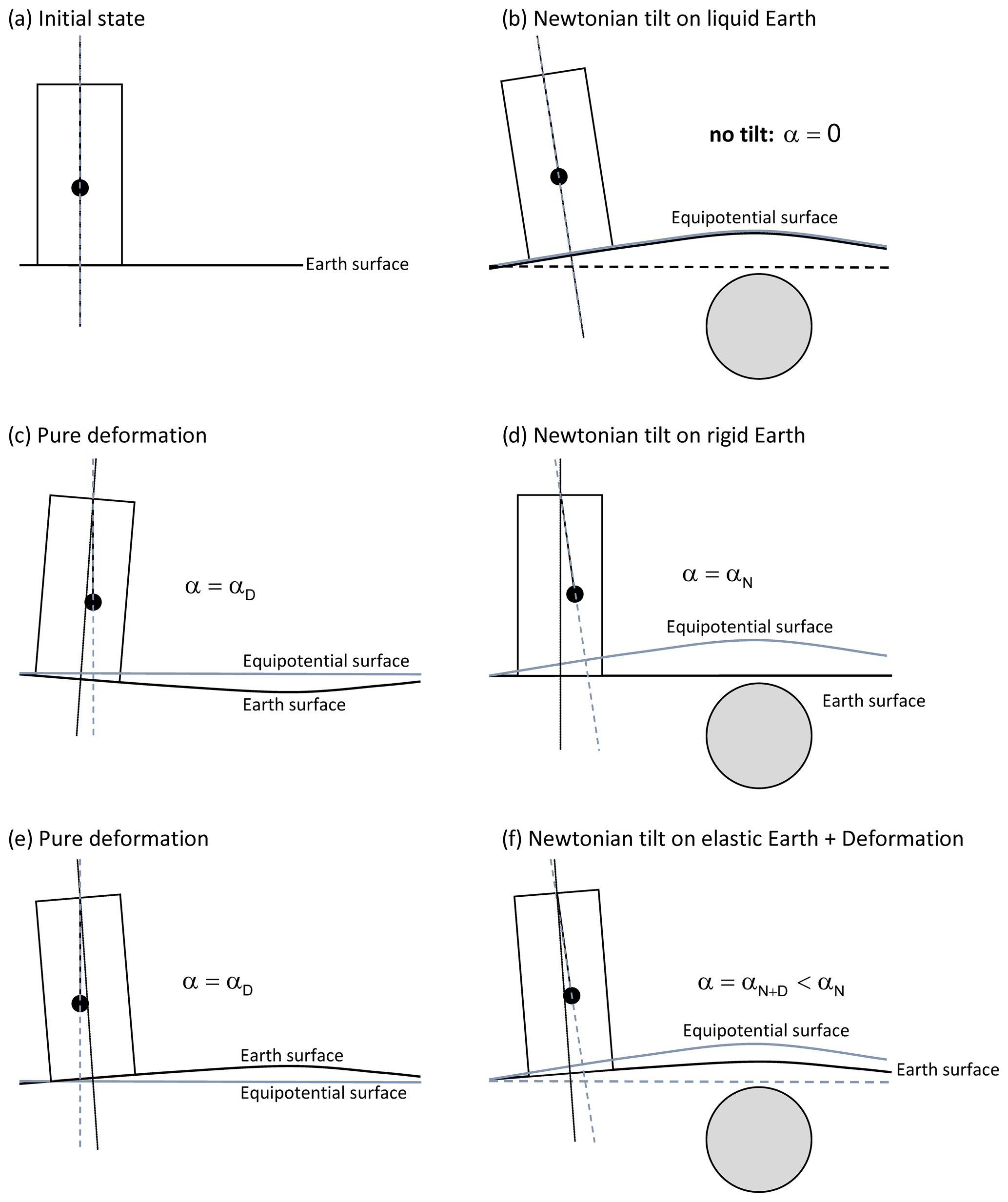
Figure 1Gravitational (Newtonian) tilt and deformation. The sphere represents an arbitrary surplus mass (interior or exterior); lines show the equipotential surface (blue solid), the planet surface (solid black), the tilt sensor axis (dotted black) and the plumb line (blue dashed). (a) Initial state, (b) no tilt on a liquid planet, (c, e) tilt due to deformation, (d) Newtonian tilt on a rigid planet, and (f) tilt on a deformable planet, including both Newtonian tilt and tilt due to surface deformation.
SGs show very low instrumental drift of a few nm s−2 per year, which can be accurately modelled by linear or exponential time functions (Van Camp and Francis, 2007). Particularly since the development of SGs, gravity monitoring has become a valuable tool for hydrogeology investigations applied in very different hydrological settings, complementing the hydrological instrumentation. Gravimeters are very sensitive to mass changes integrated at a local scale (e.g. Van Camp et al., 2017). Time-lapse microgravity surveys and SG time series provide useful estimates of water storage changes (e.g. Van Camp et al., 2006; Davis et al., 2008; Krause et al., 2009; Longuevergne et al., 2009; Creutzfeldt et al., 2010; Lampitelli and Francis, 2010; Hector et al., 2015; Güntner et al., 2017). These techniques have also been successfully applied in karst environments (e.g. Jacob et al., 2009; Fores et al., 2014; Champollion et al., 2018; Mouyen et al., 2019; Watlet et al., 2020).
In contrast, tiltmeter signals predominantly reflect the response on crustal deformation. Tiltmeter observations have widely been used for hydrogeological studies. Herbst (1979) reports tilt signals in the period range of several days obtained from Askania borehole tiltmeter measurements in Zellerfeld–Mühlenhöhe (Germany) which occurred during precipitation events or during snowmelt periods. He explained the tilt response by lateral fluctuations in the fracture water level inducing pressure differences in adjacent fracture systems, which consequently cause the elastic bending of rock structures. Jacob et al. (2010) studied water storage dynamics in the karst area of the Larzac plateau (France). Finite element modelling suggests that deformation due to water pressure changes in fractures is the most reasonable mechanism for explaining observed tilts after heavy precipitation. Tenze et al. (2012) investigated the effect of underground karstic water flow on tilt that was observed by two horizontal pendulums in the Grotta Gigante (Italy) and revealed a linear relation between the maximum tilt and the amount of water entering the karst system during flood events. Lesparre et al. (2017) interpreted tiltmeter observations inside the Fontaine de Vaucluse karst system as the infiltration effect of water after rainfall, which changes the pressure in fractures and consequently induces deformation.
Active pumping or injection experiments at different spatial scales have proven the high sensitivity of tilt to pore pressure changes (Weise, 1992; Kümpel et al., 1996; Weise et al., 1999; Fujimori et al., 2001; Jahr et al., 2008; Jahr, 2018). Within the framework of the large-scale injection experiment at the German Continental Deep Drilling Program (KTB) deep drilling site, Jahr et al. (2006a, b; 2008) studied the surface deformation due to fluid-induced stress changes by borehole tiltmeter array observations. They detected tilt signals with magnitudes between 450 and 700 nrad after 3 months of water injection and interpreted the observations as the deformation effect extending from the upper crust to the surface being caused by induced pore pressure changes. Jahr et al. (2009) analysed high-resolution (1 nrad) tilt observations at the Geodynamic Observatory Moxa (Germany), revealing a strong correlation of tilt signals with ground water level changes. All these studies show that pore pressure changes due to water content variations in the subsurface, e.g. as result of precipitation or ground water level variations, can induce tilt.
The Central Institute for Meteorology and Geodynamics (ZAMG, Austria) has operated the superconducting gravimeter (SG) GWR-C025 since 1995 within the framework of the Global Geodynamics Project (GGP; Crossley et al., 1999) and later the International Geodynamics and Earth Tide Service (IGETS; Voigt et al., 2016). After terminating a gravity time series at Vienna (Austria) extending over 12 years, the SG was moved to the Conrad Observatory (CO, Austria) in autumn 2007, starting a gravity time series over 11 years that lasted until November 2018. Looking at the non-tidal contribution to gravity variations revealed a much larger hydrological impact on the time series at CO than at Vienna. This is obviously due to complex water infiltration processes taking place after long-lasting rain or rapid snowmelt (Mikolaj and Meurers, 2013) because CO is located in a karst area, where processes are probably even more complicated than in other hydrogeological contexts. Heavy rain and rapid snowmelt cause long-term (a few weeks) residual features, the source of which could not be unambiguously identified so far. The installation of two tiltmeters in 2014 provided new insight into possible scenarios of hydrological water transport at CO by comparing tide-free SG and tilt time series, which is subject of the investigation subsequently reported.
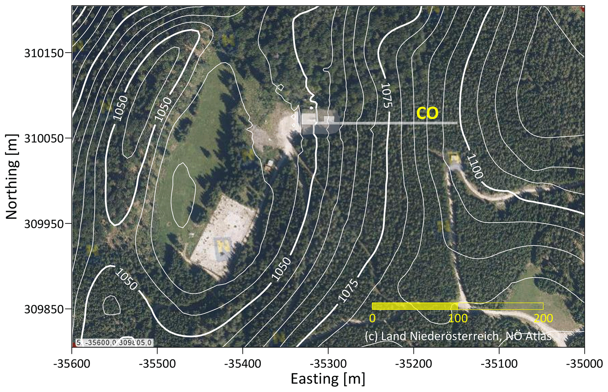
Figure 2Map of the close surroundings of Conrad Observatory (© Land Niederösterreich, NÖ Atlas). Contour lines represent the topography elevation (metres) of a high-resolution digital terrain model (DTM) used for modelling. The outline of the observatory, including the 150 m long tunnel, is displayed as well. Details are presented in Fig. 3.
The Conrad Observatory is a geophysical–geodynamic research facility located 60 km SW of Vienna (Austria) in a carbonate region belonging to the eastern foothill of the Eastern Alps, close to the top of the Trafelberg mountain at an elevation of 1050 m. The Trafelberg mountain itself is part of the Northern Calcareous Alps and shows a complicated nappe structure consisting of Main Dolomite and Wetterstein/Gutenstein limestone (Blaumoser, 2011; Bryda and Posch-Trözmüller, 2016). Three karstic caves are known in the wider surroundings of the observatory (Hartmann and Hartmann, 2000). No natural springs exist on Trafelberg itself (Deisl et al., 2014). Therefore, karstic phenomena like complex underground drainage systems, karst aquifers, caves and cavern systems, as well as sinkholes, are expected to be present. Figure 2 shows the observatory surroundings. The broad local topography low centred 100–200 m west of the observatory probably reflects a sinkhole filled by sediments today. Refraction seismic and geoelectric surveys estimate the maximum depth to consolidated rocks to be 30 m (Sirri Seren, personal communication, 2012).
The observatory consists of a building (ceiling height of about 4 m) for offices/laboratories and a 144 m long and 3 m wide tunnel drilled in an E–W direction (Fig. 3). In one of the laboratories, a massive concrete pier is directly connected to solid rock for gravimeter installations. Prior to the construction of the building, a huge amount of rock was blasted out of the terrain. Before the concrete foundation plate was made for the building, the remaining cragged and rough rock surface was levelled by a gravel sheet. After completion of the building, the space next to and above the building was refilled by the excavated material in order to restore the original terrain shape. Above the SG, coverage amounts to approximately 7 m. The gravel sheet below the building is a potential water storage reservoir influencing the observed gravity. The tunnel surroundings consist of solid rocks; the coverage increases towards the east from 15 m at the tunnel entrance to about 55 m at the end, with approximately 33 m at the tiltmeter pier. Given the geometry and orientation of the tunnel, cavity effects are expected to be the strongest in N–S tilts.
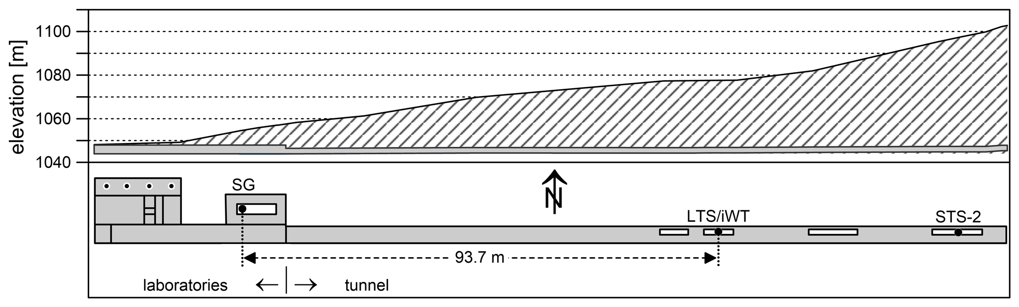
Figure 3Vertical section and ground plan of the Conrad Observatory. Sensor positions are displayed by black dots. Small dots indicate boreholes of different depth.
Gravity data are sampled with 1 Hz by two redundant digital volt meters (DVMs) for detecting the possible long-term scale factor changes in the DVMs. SG calibrations by co-located absolute gravimeter (JILAg-6; FG5) observations took place twice a year and were supported by numerous SG/Scintrex CG-5 relative gravimeter intercomparisons (Meurers, 2012, 2018a). Commonly, the SG scale factor (SF) is assumed constant as long as the hardware (e.g. coil geometry and transfer function) does not change (Goodkind, 1999), which allows for an averaging of the calibration results (Van Camp et al., 2016; Crossley et al., 2018). Systematic SF changes, if present and larger than 0.1–0.2 ‰, are reliably detectable by studying the temporal M2 tidal parameter modulation of successive tidal analyses over 1 year intervals. Combining calibration results and M2 parameter modulation studies (Meurers et al., 2016) proved the accuracy and time stability of the SG scale factor at CO to be far below 1 ‰ (Meurers, 2018a).
In August 2014, the Geodetic and Geophysical Institute (GGI, Sopron, Hungary) installed a 5.5 m long Michelson–Gale-type interferometric water level tiltmeter (iWT), recording at only one end of the tube, designed by the Finnish Geodetic Institute (FGI; Ruotsalainen et al., 2016a, b; Ruotsalainen, 2018), on a 6 m long pier in the middle of the tunnel, about 94 m away from the SG. Continuous tilt measurements started at CO in order to monitor geodynamical phenomena like microseisms, free oscillations of the Earth, earth tides, mass loading effects (ocean tidal and atmospheric loading) and possible crustal deformations. In July 2015, a Lippmann high-resolution tiltmeter (HRTM) 2D pendulum tilt sensor (LTS) with <1 nrad resolution (https://www.l-gm.de/en/en_tiltmeter.html, last access: 23 November 2020) was installed by GGI close to the iWT on the same pier (Papp et al., 2019). This set-up of instruments based on different physical principles (relative height change of a level surface vs. inclination change of the plumb line) allows for a comparison of the response of tiltmeters with long (several metres) and short (a few decimetres) base lengths. While iWT monitors E–W tilts, LTS provides both N–S and E–W tilt time series. The tiltmeter sampling rate is 1 Hz (LTS) and 15 Hz (iWT) respectively. The scale factor of the LTS tiltmeter is factory based. The iWT scale factor is absolute and based on optical interferometry in the CO station condition. The iWT tiltmeter detects crustal tilt from water level variations at one end of the tube by interference phase values, which are converted to tilt by a conversion factor based on laser wavelength, refraction coefficient of water and tube length of the tiltmeter (Ruotsalainen, 2018).
All instruments are underground installations in a thermally stable environment. The tiltmeters are located approximately 33 m below ground surface. Based on theoretical calculations by Harrison and Herbst (1977), Bonaccorso et al. (1999) estimate that the maximum amplitude of thermoelastic tilt of the rocks beneath the surface decays towards zero at 10 m depth. Even if this approach might underestimate the real thermoelastic effect, as shown by experiments with shallow borehole tiltmeters at different depth (Bonaccorso et al., 1999), the coverage of 33 m should reduce thermoelastic tilt deep in the tunnel.
In order to investigate atmospheric and precipitation effects on gravity, a wide range of meteorological parameters are monitored by mobile and permanent sensors as follows:
-
The air pressure, air temperature and humidity sensors located outside, above the laboratory; an air pressure sensor included in the SG-acquisition system; the air pressure, temperature and humidity sensors integrated within the LTS tiltmeter housing; and additional air pressure and temperature sensors in the observatory labs and the tunnel.
-
A tipping bucket rain gauge model AP-23 (Anton Paar GmbH, Austria) with 0.1 mm resolution.
-
A disdrometer (Adolf Thies GmbH & Co. KG, Germany) measuring the size and fall speed of precipitation particles and classifying the precipitation type by the surface synoptic observations (SYNOP) code.
-
A 3D ultrasonic anemometer (Adolf Thies GmbH & Co. KG, Germany).
-
A SSG-2 snow scale (Sommer Messtechnik, Austria) monitoring the weight of the snow pack in front of the observatory and providing snow water equivalent data. The snow scale was out of operation between 1 January and 15 March 2018. Missing data has been replaced by information from a nearby (150 m SW of the observatory) snow height sensor.
To separate small amplitude gravity and tilt signals of different physical origins, like, for example, hydrological response or tectonic signals, we need to subtract the tidal effects which dominate the gravity and tilt time series. The atmospheric pressure and polar motion are also known to contribute remarkably to temporal gravity and tilt variations, although much less so than the tides. Both the SG and the tiltmeters are relative instruments and, hence, may exhibit instrumental drift. Generally, the SG drift is expected to be only a few nm s−2 per year. Absolute gravity observations performed at CO did not reveal any significant instrumental drift of the SG until now (Meurers, 2018b). However, the tilt sensors show strong drift dominated by linear trends up to −10 and +2.5 µrad yr−1 for the LTS and iWT sensors, respectively, and by possible thermal origin. Therefore, the gravity and tilt time series must be properly processed to derive the residual time series. Preprocessing and determination of gravity/tilt residuals followed the procedure which is standard for SG time series (Hinderer et al., 2007). To decimate the 1 Hz samples to 1 min or 1 h samples, we applied numerical filters g1s1m and g1m1h, respectively (http://www.eas.slu.edu/GGP/ggpfilters.html, last access: 23 November 2020). Local tide models in the diurnal and sub-diurnal frequency bands and air pressure admittances were derived individually for each sensor from tidal analyses by applying ETERNA v3.4 and ETERNA-x et34-x-v80 (Wenzel, 1996; Schüller, 2020). Tidal parameters of theoretical body tide models (e.g. Dehant et al., 1999) are used for long-period tides. The following preprocessing steps had to be applied additionally for the tilt sensors:
-
Interpolation of 15 Hz iWT data to 5 Hz samples and decimation of 5 Hz data to 1 Hz samples by using a Gaussian operator with 61 coefficients equivalent to 1 min time length.
-
Correction of transient signals due to thermal disturbances in the tunnel, which are very small but happen occasionally during maintenance work. Until August 2017, an episodic temperature increase of a few 0.01 ∘C inside the LTS was observed by the built-in sensor, generating tilt signals much larger than the tidal signal. The temperature correction was based on linear or nonlinear models, depending on the thermal event. Since August 2017 both tilt sensors have been isolated from the temperature fluctuation in the tunnel by styrofoam sheet insulation around the tiltmeters, which effectively suppresses the thermal disturbances.
-
Correction of steps, in particular for iWT data, by applying TSoft (Van Camp and Vauterin, 2005) and our own codes. Due to its incremental measuring principle, iWT sometimes suffers from interference phase cycle slips; the correct interpretation of the interferogram phase fails if the phase change between two consecutive interferograms is larger than one interference phase value, typically of 203.6 nm. This happens during large earthquakes when ground motion is so fast that the fluid level of the instrument cannot follow the fast and large seismic surface wave arrivals in the first minutes.
-
Removal of the low-order polynomial trends.
The local tide model for gravity matches the theoretical body tide models (e.g. Dehant et al., 1999; Mathews, 2001) and the ocean tide loading predictions provided by Bos and Scherneck (2017) almost perfectly (e.g. CSR4.0 in Eanes, 1994; GOT00.2 in Ray, 1999; TPXO7.2 and TPXO9 in Egbert and Erofeeva, 2002; FES2004 in Lyard et al., 2006; EOT11a in Savcenko and Bosch, 2011; DTU10 in Cheng and Andersen, 2010; HAMTIDE in Taguchi et al., 2014; and NAO99 in Matsumoto et al., 2000). This is due to the high accuracy of both the SG scale factor determination (0.2 ‰) at CO (Meurers, 2018a) and the tidal analysis, which is based on time series longer than 10 year (Meurers, 2018b). The formal errors of gravimetric factors are far below 0.1 ‰ for the main tidal constituents. The root mean square (RMS) error of a single observation estimated from the tidal adjustment residuals, which was calculated by using the adjusted tidal parameters, is 0.6 nm s−2 or 0.9 ‰ of the tidal peak-to-peak M2 amplitude only.
Local tide models for the tilt sensors are much less accurate. The RMS errors of a single observation derived from the least squares adjustment (LSQ) of tidal parameters range from 1.6 to 2.9 nrad, which is of the order of about 2 %–4 % of the peak-to-peak M2 tidal signal. Also, much less data (LTS N–S – 21 700 hourly samples within 1064 d; SG – 83 500 hourly data within 3512 d) could be used for tidal analyses. Table 1 compares the tidal parameters of the main tidal groups for the LTS and iWT tilt sensors. The LTS N–S component turns out to be heavily disturbed by non-tidal excitation, particularly in the diurnal band, while the E–W components do not deviate considerably from the body tide predictions. We also analysed the data a priori corrected for atmospheric and induced non-tidal oceanic loading contributions (Boy et al., 2009) provided by the School and Observatory of Earth Sciences (EOST) Loading Service (http://loading.u-strasbg.fr/, last access: 23 November 2020). After correction, the non-tidal tilt anomaly in the diurnal band still persists. However at CO, ocean loading corrections based on the TPXO9 model (http://holt.oso.chalmers.se/loading/, last access: 23 November 2020) do not essentially reduce the deviation of the observed tilt factors from the body tide predictions. Because the tunnel axis is oriented in an E–W direction, the N–S component corresponds to the tilt perpendicular to the tunnel axis and, therefore, is extremely sensitive to cavity effects (King and Bilham, 1973; Harrison, 1976; Agnew, 1986). This is the most likely reason for anomalous tidal parameters in the N–S tilt, particularly in the diurnal band where tidal N–S tilt wave amplitudes are small (<5 nrad). The high LTS/iWT ratio of the E–W tilt factors hints at calibration errors. LTS tilt factors are about 6 %–11 % higher than those of the iWT, i.e. the tidal parameters are probably also affected by unknown transfer functions of the tilt sensors. However, we cannot exclude the idea that cavity effects play a role as well, as the respective tilt sensors are not at exactly the same place and have different base lengths. In order to consider all these problems properly, sensor-dependent tidal models have been used for the tilt residual determination.
Table 1Comparison of tidal parameters derived from tilt time series at CO. Theoretical body tide model as per Dehant et al. (1999). Note: LTS – Lippmann HRTM 2D pendulum tilt sensor; iWT – interferometric water level tiltmeter.

Air pressure also has a strong impact on observed tilts, predominantly due to surface loading (e.g. Rabbel and Zschau, 1995) and directly results in surface and subsurface deformation, depending on the spatial scale of load masses (e.g. Llubes et al., 2004). Air pressure changes are caused by air packages with different densities and spatial extent passing the station. Therefore, air pressure signatures in tilt time series are expected to be frequency dependent, as it is well known from gravity records. Loading by accumulated water or snow produces deformation in a similar way. Hence, it is worth studying the air pressure admittance function for the tilt. Air pressure tilt admittances for tidal frequencies were calculated in a joint adjustment, together with the tidal parameters by ETERNA-x et34-x-v80 software (Schüller, 2020). The results in Table 2 represent the diurnal and semidiurnal frequency band only because long-period tides were not included in the adjustment. To obtain higher frequency information, we investigated the frequency dependence of the air pressure admittance by applying a cross-spectral analysis (Bendat and Piersol, 2010) on several detided tilt time series covering intervals between 2 and 21 d (10 d on average) for both LTS N–S and LTS E–W. For LTS N–S, the air pressure admittances confirm the number resulting from the tidal analysis (Table 2) obtained in the diurnal and semidiurnal frequency band. Clear time variability is seen at frequencies beyond 0.3 mHz (equivalent to a period of about 1 h), which is of instrumental origin. Therefore, separating physically meaningful signals from instrumental artefacts is not possible in the frequency range larger than 0.3 mHz. Details are provided in Appendix A. However, at long periods, the air pressure signal in the tiltmeter time series is due to geophysical/geodynamical reasons, which are probably dominated by deformation due to air pressure loading. Here, the admittance is again much higher for the N–S tilt than for E–W tilt (similar to that shown in Table 2), which is as expected due to the cavity effect. We will come back to this in Sect. 5.1 when we discuss the tilt response to water mass load on the terrain surface.
Table 2Air pressure admittances in the diurnal and semidiurnal frequency band for the tilt sensors derived from tidal analysis.
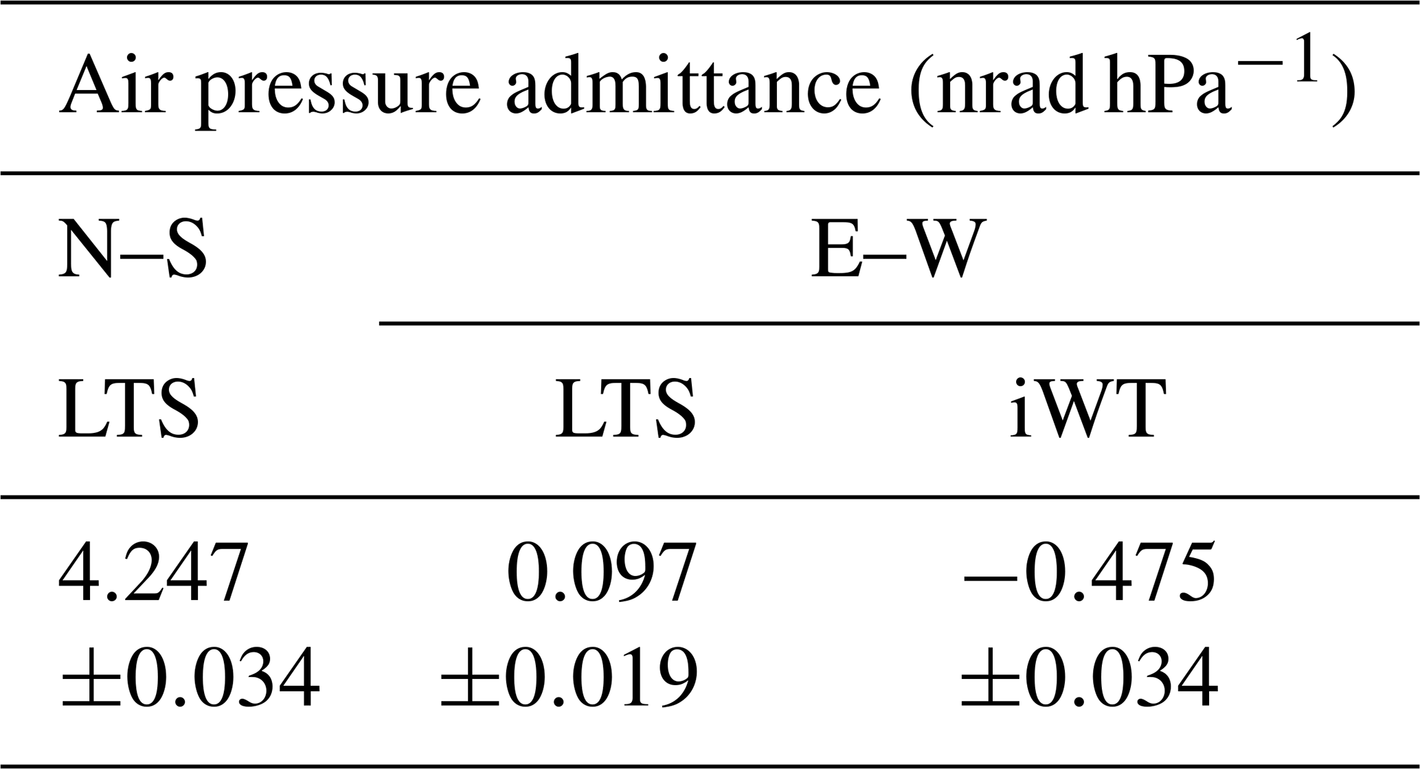
Figure 4 presents the final gravity and tilt residuals of the common observation period extending from end of April 2016 until mid-November 2018. Comparing the residuals with cumulative rain and snow (water equivalent) shows an obvious link between both short- and long-term residual anomalies related to different hydrological processes.
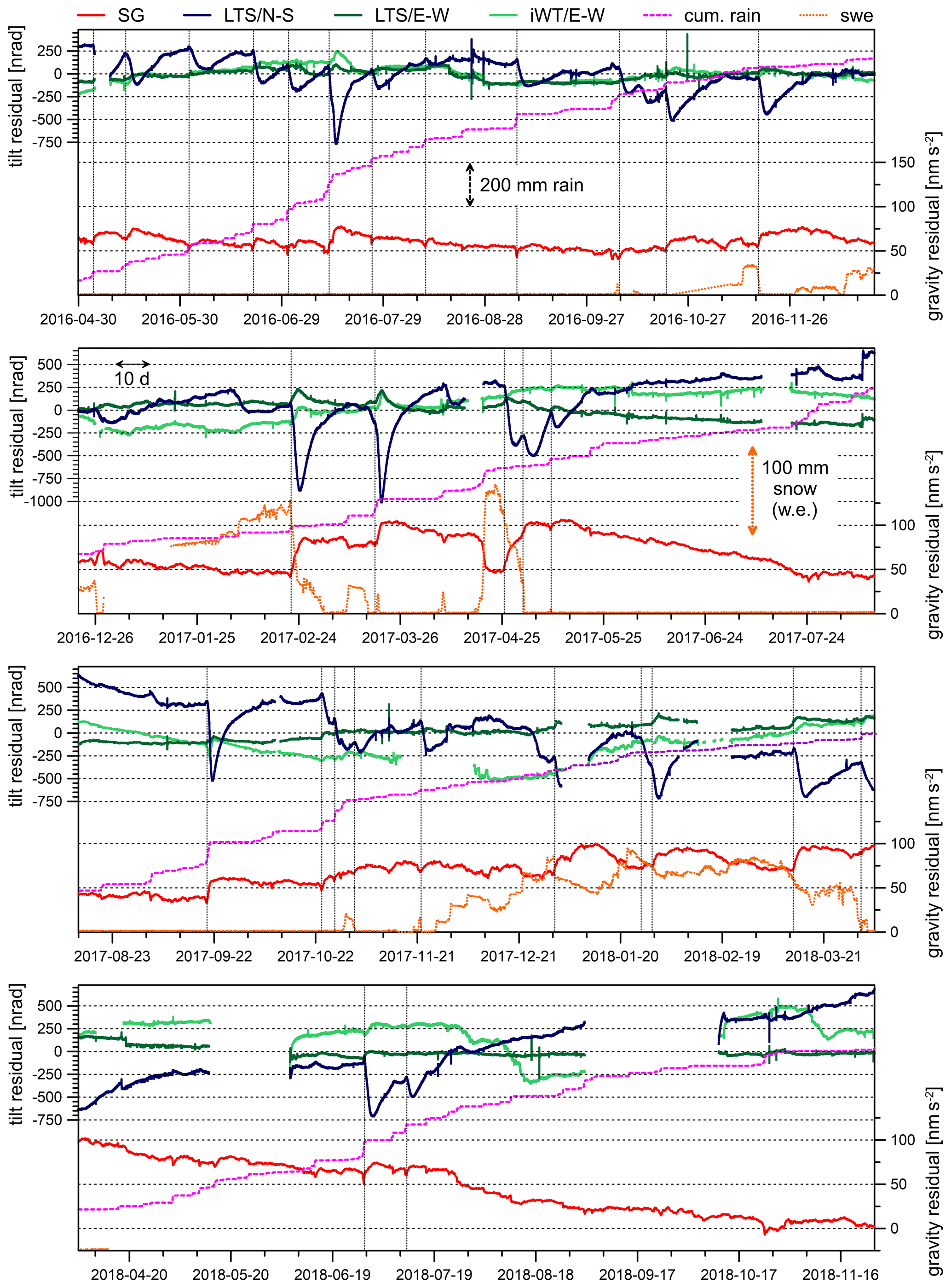
Figure 4Comparison of gravity and tilt residuals, showing gravity (red), N–S tilt (LTS – dark blue), E–W tilt (LTS – dark green; iWT – light green), cumulative rain (dashed magenta line); snow water equivalent (dotted orange line). Scales for rain and snow (water equivalent) are indicated by arrows. Vertical dotted lines mark the onset of hydrologically induced long-term events.
5.1 Short-term signatures (water accumulation phase)
Figure 5 presents a typical example of a heavy rain event on 11 July 2016. The SG residuals decrease sharply and exactly at the time when rain starts. This is mainly due to the Newtonian effect of rainwater distributed at the terrain surface, above the instrument. Actually, due to their high precision, SGs reveal these effects not only in the case of heavy rain events but also in the case of light rainfall even smaller than 1 mm h−1. The gravity residual drop can be very well estimated by multiplying the cumulative rain with a rain admittance factor based on a digital terrain model in a high spatial resolution (Meurers et al., 2007). The rain admittance depends on terrain geometry, SG sensor location and on the area of rainwater accumulation. At CO, the rain admittance varies between −0.26 and −0.29 nm s−2 per 1 mm rain for accumulation areas between 104 and 102 km2 (Fig. 6a). Correcting for the Newtonian effect of cumulative rain removes the gravity response to rain almost perfectly (Fig. 5; light red line). Of course, the rain admittance concept works only during the accumulation phase, while it fails when the residuals recover their initial level after rainfall.
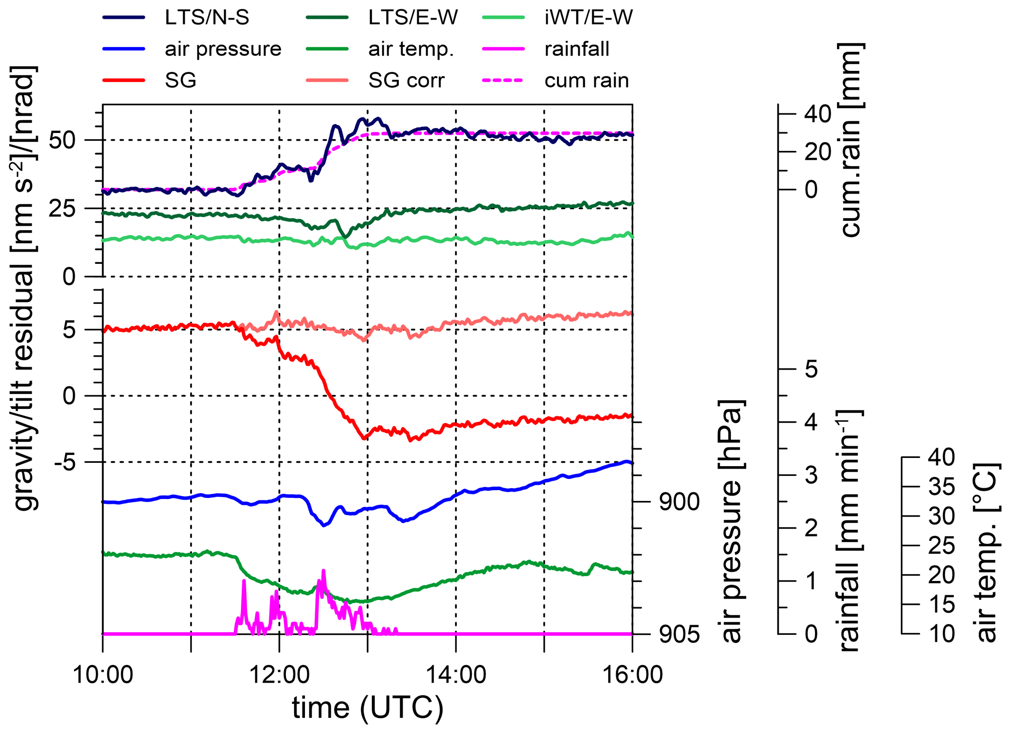
Figure 5Effect of heavy rain on gravity and tilt at CO on 11 July 2016. Gravity and N–S tilt residuals show patterns clearly related to cumulative rain, while E–W tilts do not, or only weakly, respond to rain. The legend indicates the following, from top to bottom: N–S tilt residuals (dark blue), E–W tilt residuals (LTS – dark green; iWT – light green), cumulative rain (dashed magenta line) scaled to fit the N–S tilt optimally, SG gravity residuals (red), gravity corrected for cumulative precipitation (light red), rainfall (magenta), air pressure (blue) and outdoor air temperature (green).
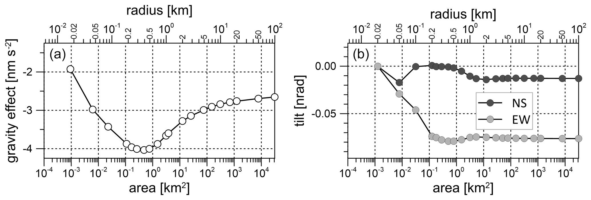
The same approach can be applied to estimate the Newtonian tilt effect of rainwater in both the N–S and E–W direction. Corresponding rain admittances turn out to be as small as nrad per 1 mm rain for the N–S tilt and nrad per 1 mm rain for the E–W tilt, respectively, if the rainfall area extends to more than 2 km symmetrically around the tilt sensor (Fig. 6b). In the case of a rain front, the Newtonian effect can be considerably larger and depends on the direction from which the rain front approaches the station. The effect of asymmetric rainfall areas extending to a line just passing the tilt sensor location provides the maximum estimate, which does not exceed nrad per 1 mm rain at CO. However, in realistic weather situations, the rain-to-tilt admittance is much smaller and depends on the velocity at which the rain front moves over the sensor. Given these small numbers, the Newtonian tilt effect of rainwater or snow turns out to be negligible at CO because it is far below the reliable resolution of tiltmeters.
Nevertheless, there is a clear and instantaneous N–S tilt response on rain (exemplarily shown by Fig. 5), which is visible in almost all (71 out of 74) heavy rain events. Tilt response on air pressure changes can be ruled out as a reason because the temporal patterns of air pressure and tilt are totally different in most cases, while tilt and cumulative rain match each other. Similar to the case of gravity, we do not observe any time delay between cumulative rain and tilt response. In contrast, tilts in the E–W direction rarely show short-term signatures that could be related to rain. In only 10 out of 48 rain events is a slight transient residual decrease visible, which, however, often starts much earlier than rain. Figure 7a shows the observed total N–S tilt offsets as a function of cumulative rain or of the surface pressure load exerted by cumulative rain at the end of the respective rain event. The average rain admittance results in 0.73 nrad mm−1, which is about 580 times larger than the value estimated for purely gravitational tilt (Fig. 6) or about 7.4 nrad hPa−1 after converting cumulative rain into surface load pressure. This corresponds to the air pressure admittance for the N–S tilt at about 0.3 mHz. Also, we find a close relation between the response of N–S tilt and gravity to short-term water accumulation at topography (Fig. 7b). The air pressure admittances for the E–W sensors are much weaker than those for the N–S tilt sensor at all frequencies, which may explain why we rarely see E–W tilt effects due to rain. Surface load (either due to air pressure or rain/snow) rarely produces clear signatures in the E–W tilts because the cavity effect is much smaller for E–W tilt than for N–S tilt. Tilt response to surface load by water accumulation evidently compares well with the tilt response to atmospheric pressure changes for both the N–S and the E–W components. The SG reflects mainly the gravitational effect of the rain/snow water, while the deformation effect on gravity (vertical displacement) at the given spatial scale is too small to be detected; in contrast, the tiltmeter responds to deformation caused by the pressure the water exerts onto the terrain surface, similarly to in case of air pressure variations. It is probably the cavity effect, which amplifies the observed tilt such that it emerges from the noise in case of the N–S component, which is oriented perpendicular to the tunnel axis at CO.
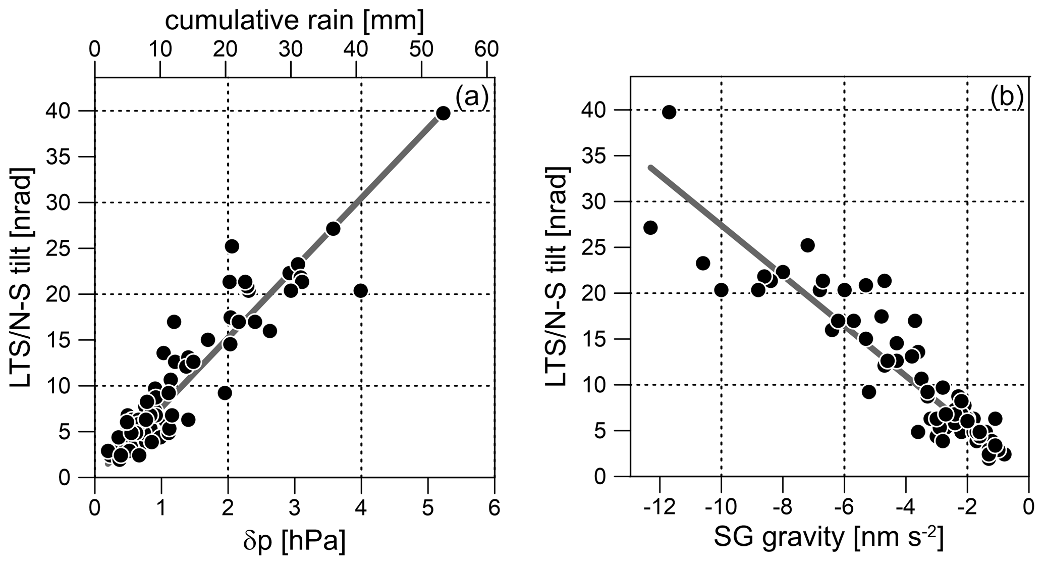
Figure 7Short-term N–S tilt and gravity residuals (water accumulation phase). N–S tilt response to cumulative rain at CO (a). Converting cumulative rain to surface pressure load reveals a tilt-to-pressure admittance of 7.6 nrad hPa−1 (solid line). Relation between gravity and N–S tilt residuals (b).
The findings above also hold in the case of solid precipitation, as shown in Fig. 8, which presents an example of gravity and N–S tilt response to pure snow accumulation. Disdrometer data (Fig. 8; coloured dots) show that almost no liquid precipitation is involved. The disdrometer provides information on the aggregate state of the precipitation particles even for extremely little precipitation. However, as indicated by the rain data (Fig. 8; magenta), liquid rain does not essentially contribute to water accumulation in the presented case study. Consequently, no essential water infiltration can take place because most precipitation is solid and air temperature remains slightly below the melting point (Fig. 8; green line). Note that heated rain gauges often report solid precipitation incorrectly and/or time delayed because the solid particles have to melt before they are counted by a bucket rain gauge. The disdrometer detects precipitation starting as snow grains and light drizzle during night and early morning with an intensity which is too small to be observed by the rain gauge. Precipitation continues as light to heavy snow from 08:00 universal coordinated time (UTC) onwards. The snow scale indicates the onset of snow cover increase at about 12:00 UTC. Gravity residuals start decreasing at the same time and reach a local minimum at about 22:00 UTC when heavy snow fall terminates. The prediction of the cumulative precipitation effect by applying the rain admittance removes the gravity residual drop almost perfectly (Fig. 8; light red line). A significant signal associated with the main snow accumulation phase is also visible in the N–S tilt residuals, which are comparable in magnitude to rainfall events (compare to Fig. 5), i.e. snow affects tilts similarly as in the case of rain, and the snow water equivalent matches the tilt time pattern if properly scaled (Fig. 8; orange line). Again, gravity and tilt react instantaneously, i.e. without time delay.

Figure 8Effect of snow accumulation on gravity and tilt at CO on 21 and 22 December 2017. The legend indicates the following, from top to bottom: N–S tilt residuals (dark blue), E–W tilt residuals (dark green), snow (water equivalent – orange) scaled to fit the N–S tilt optimally, SG gravity residuals (red), gravity corrected for cumulative precipitation (light red), air pressure (blue) and outdoor air temperature (green).
The short-term residual anomalies can therefore be well explained by the accumulation of precipitation on the terrain surface and in the adjacent topsoil. While the gravity response reflects the gravitational acceleration of accumulated water/snow mass, the N–S tilt response is interpretable as the pure deformation effect caused by the pressure the water mass exerts on the terrain surface. Similarly, as in the case of atmospheric pressure changes, the cavity effect enhances observed tilts in the N–S direction much more than those oriented E–W. If the accumulation phase is short, as in the case studies discussed so far, we do not expect considerable water percolation into the subsurface to change the pore pressure there.
5.2 Long-term signatures (water percolation phase)
It is common to most rain events that, after rainfall, a slow discharge process brings the gravity residuals back to their initial level (Fig. 4). However, in some events, the residuals exceed the initial level remarkably, in particular after long-lasting rain or rapid snowmelt. We interpret this as the response to downward water flow (infiltration) from the terrain surface into the ground until water is stored somewhere below the SG sensor. This process probably starts as soon as the subsurface is sufficiently saturated by rain or snowmelt water and, therefore, needs a certain threshold to be triggered. Mangou (2019) estimated that about 20 mm water accumulation within the past 3 d is required. However, this number is a rough estimate. The degree of saturation and meteorological conditions (e.g. evaporation rate, etc.) plays a role as well.
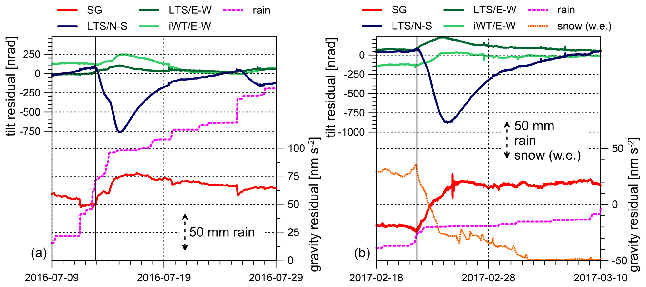
Figure 9Long-term gravity and tilt residual signals caused by hydrological processes after heavy and long-lasting rain (a) and during rapid snowmelt (b). N–S tilt residuals (dark blue) and E–W tilt residuals (LTS/dark green and iWT/light green). SG gravity residuals (red). Cumulative rain (dashed magenta line), snow (water equivalent; dotted orange line). Scales for rain and snow water equivalent indicated by arrows. The black vertical line shows the onset of the long-term residual anomaly.
Interestingly, all of these events are associated with simultaneous long-term tilt anomalies. Almost at the same time that the SG gravity residual starts to increase, we see strong signals in the tilt time series as well. The N–S tilt always shows a steep residual drop, and the E–W tilt residuals (in particular LTS) increase temporarily but with much less amplitude. E–W tilt signals are often masked by noise. All events in which we identified long-term signatures both in gravity and tilt residuals are marked by dotted vertical lines in Fig. 4. Figure 9 exemplarily enlarges into a long-lasting rain event (Fig. 9a) and into a rapid snowmelt event (Fig. 9b). Once N–S and E–W tilts have reached their extremes, they return to their former level; this is a process which takes about 14 d or more. The short-term signals discussed in Sect. 5.1 are visible in Fig. 4 too, even though they are very small compared to the long-term signal. The long-term anomalies start when sufficient water has percolated downwards into the subsurface, either after heavy/long-lasting rainfall or in case of rapid snowmelt. Quantifying the long-term anomalies is not easy because the tilt/gravity response to long-term water transport depends on the overall subsurface saturation for which we have no constraints based on observations. However, there is a significant relation between the long-term residual anomalies observed in the tilt and gravity residuals (Fig. 10a). Tilt residual anomalies always have either negative (N–S tilt) or positive (E–W tilt) signs. The absolute value of the anomaly amplitudes increases with the amplitude of the gravity residual anomaly, whereby the N–S residual anomaly amplitude is about 7 times larger on average than that of E–W residuals (Fig. 10b).
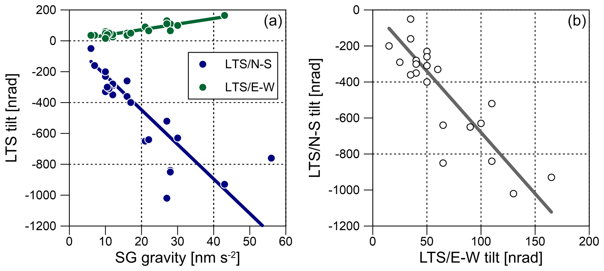
Figure 10Long-term tilt (LTS) and gravity residuals (water percolation phase). Relation between the amplitudes of long-term tilt and gravity residual anomalies (a). Relation between the amplitudes of long-term N–S and E–W tilt residual anomalies (b). The average ratio of N–S to E–W tilt is −0.15.
In the following, there are a few candidates for water storage volumes at CO:
-
the gravel layer below the concrete foundation plate of the underground observatory building and the laboratories in front of the tunnel,
-
fissures and cracks in the solid rock, or
-
perhaps a karstic volume filled by water after heavy rain/snowmelt.
We first investigate whether a locally limited surface or subsurface mass is able to produce the observed long-term tilt/gravity residuals. Comparing the E–W and N–S tilt data, the amplitude ratio of the long-term residual anomalies turns out to be about −0.15 on average (Fig. 10b). E–W tilt is always positive; N–S tilt is always negative (Fig. 10a). If the observed tilt is solely due to gravitational attraction by a volume of stored water, then the source must be located on a line with an azimuth of about 170∘. Based on the high-resolution digital terrain model (DTM) of the area (Meurers et al., 2007), the existence of any surface depression capable of cumulating enough run-off water mass (Kalmár and Benedek, 2018) to generate the observed tilts can be checked. Figure 11 shows that there are two local topographical lows (valleys) along the profile. However, due to their distances from the observatory, an enormous amount of water (>105 m3) would have to be accumulated in a corresponding cell of the DTM (determined by the azimuth) to generate even a fraction (1 nrad) of the observed tilts (up to ∼1000 nrad). Regarding the horizontal extension of such a cell (50 m × 50 m), a 40 m water height would be required to provide this volume. The same holds for a fictitious topographical reservoir located in the very close vicinity (<50 m) since about 1000 m3 of water is necessary for the same tiny (1 nrad) gravitational tilt. This volume of water is supplied by 1 mm of rainfall on 1 km2, but obviously even this amount cannot be caught and concentrated near to the observatory, as one can conclude from Fig. 2 which shows the elevation contour lines. The estimations above are based on forward gravitational modelling of the horizontal attraction of mass columns (e.g. Papp and Benedek, 2000) representing the water mass placed on top of the topographic mass columns. However, there is no evidence of such a large basin next to CO in the required azimuth. Another point the source modelling shows is that along this azimuth no spherical volumes representing one single subsurface cavity either partially or completely filled by water would simultaneously explain both the gravity and tilt residuals of the events shown in Fig. 4.
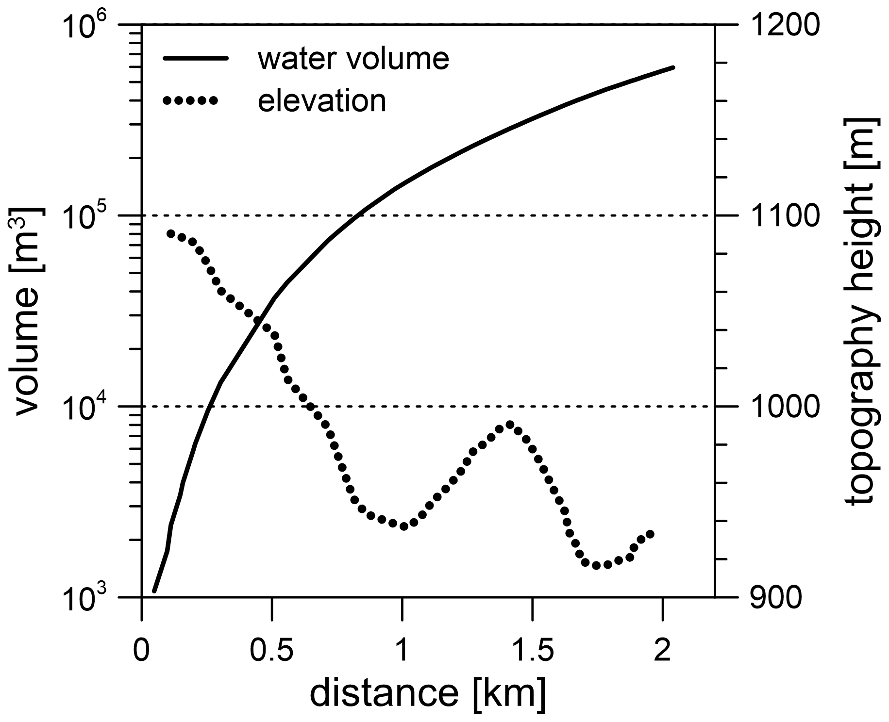
Figure 11Estimation of the magnitude of water volume (black) capable of producing 1 nrad tilt if it was purely Newtonian. The dotted line shows the cross section of the topography in the specific azimuth defined by the E–W and N–S tilts detected during rainfall events.
Therefore, regarding the long-term residual variations, a pure Newtonian effect of one single source (e.g. one single karstic cave filled by water) representing the water accumulation near the gravity and tilt sensors can be ruled out because of the following two reasons:
-
model calculations show that, contrary to the short-term anomalies, no reasonable solution exists to explain the observed long-term tilt and gravity effects, and
-
the onsets of the long-term residual features in gravity and tilt do not coincide exactly in time.
Deformation by increasing pore pressure after water infiltration into the subsurface is the most reasonable explanation for the observed tilts. Actually, the observed long-term N–S tilt response (Figs. 4 and 9) is very similar in shape to the observations reported by Herbst (1979) or by Jahr et al. (2006a, b) in one of the tilt records of a borehole tiltmeter array established at the KTB deep drilling site (Germany).
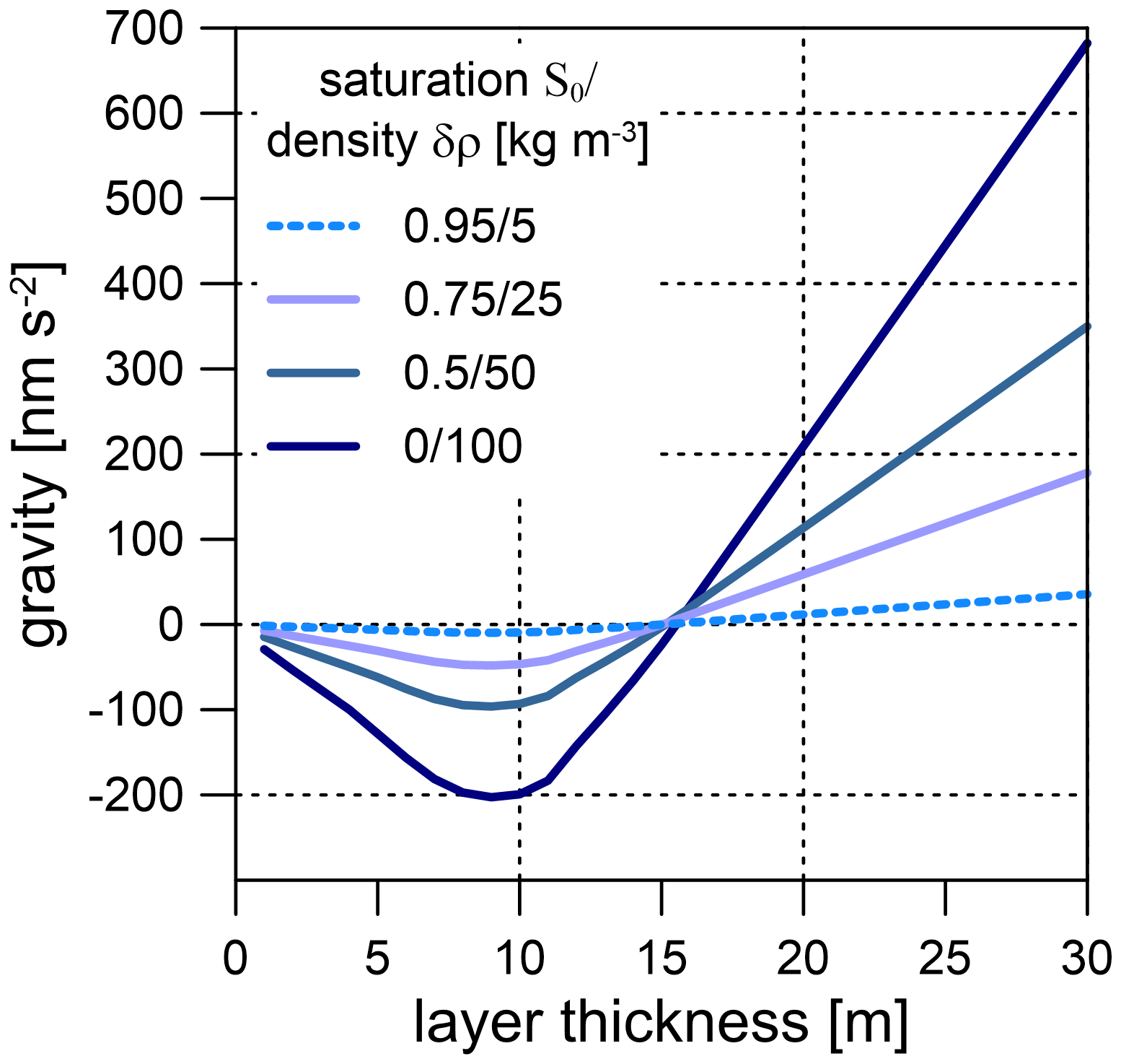
Figure 12Modelled gravity of a layer with constant thickness as function of the layer thickness and the degree of initial soil/rock saturation (for an explanation, see the text).
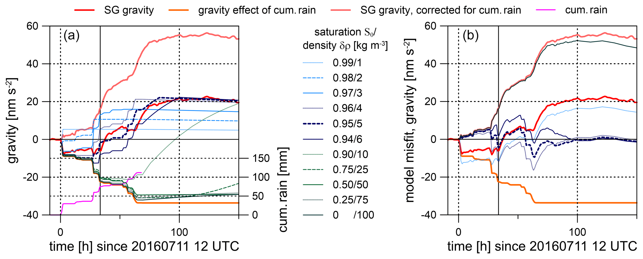
Figure 13Modelled gravity response for a real cumulative rain function (monitored between 11 and 14 July 2016) for different degrees of initial saturation S0. Model response (a) and model mismatch (b). Observed gravity (red), cumulative rain (magenta) and gravity effect of cumulative rain (orange) are shown for comparison. Black vertical lines indicate the onset of the long-term anomaly. The right panel displays results only for the best-fitting models () and for S0=0 and S0=0.99.
Certainly, the hydrological water transport process is very complex at CO. Due to the high sensitivity and extremely low and almost linear instrumental drift of SG sensors, the SG gravity residual very clearly reveals the Newtonian effect (vertical component) of the water mass transport involved in hydrological charge and discharge processes. We modelled the gravity effect by a simple layer in order to estimate the maximum observable gravity residual drop as a function of the layer thickness and of the degree of initial soil/rock saturation. The upper layer boundary coincides with the terrain surface; the lower boundary is defined by shifting the terrain surface vertically downwards. The topography is represented by the same DTM with a high spatial resolution, in particular in the vicinity of the SG, as already has been used for the rain admittance calculations. The effective layer density δρ results from Eq. (1) as follows:
with ρw and ϕ denoting water density and rock porosity, respectively. S0 and S describe the saturation of the pore volume before (initial saturation) and after downward water mass transport. The model takes into account that water storage is impossible within the volume occupied by the observatory building/tunnel, the foundation plate of the building and the gravimeter pier. Figure 12 shows the modelled gravity as a function of layer thickness for S=1 and different degrees of initial saturation S0, assuming a porosity of ϕ=0.1. The effective layer density is 100 kg m−3 for initially completely dry rock (S0=0). Alternatively, we can interpret Fig. 12 also as the gravity effect of the same layers as a function of layer thickness but for different porosity, assuming S=1 and S0=0. Then, the layer density provided in the legend of Fig. 12 translates into porosity after division by 1000. The minimum gravity residual occurs at a layer thickness of about 9 m in each case, whereby the drop in amplitude increases with decreasing degree of initial saturation S0. Given the terrain model geometry at CO, the minimum residual drop in amplitude never exceeds about 200 nm s−2 (S=1 and S0=0) at the SG site. However, observed numbers are much smaller. For all events shown in Fig. 4, the residuals never drop by more than about 10 nm s−2, which indicates a high degree of initial subsurface saturation or porosity lower than assumed in the model. We investigated the period from 11 and 14 July 2016 (Fig. 9a), during which a series of consecutive heavy or long-lasting rainfall events occurred, in more detail. Simultaneous to the first rainfall on 11 July 2016, the gravity residuals decreased by about 8 nm s−2 and remained nearly at this level after rain has stopped. More heavy rain events followed, separated by a couple of hours (Fig. 13a). The residuals always drop instantaneously at the onset of each event but start to increase a short time later. In total, they increase to a much higher level than what they started from at the beginning, although more and more rain is accumulated. We developed a time-lapse model and compared the time-dependant model response with observed gravity residuals. Unfortunately, we cannot constrain our model by hydrological observations. Therefore, the very simplistic model is based on the following assumptions:
-
A constant porosity of ϕ=0.1 and a constant degree of saturation S=1, which translates into a subsurface density δρ, according to Eq. (1). That means that the water percolating downwards fills the pore volume completely. The choice of the porosity seems to be reasonable. Jacob et al. (2009) report values between 0.04 and 0.12 in a karstic environment (Larzac plateau, France).
-
Rainwater is assumed to percolate into the subsurface as a layer of spatially constant thickness H(t). The upper layer boundary coincides with the terrain surface as before, while the lower boundary results from shifting the terrain surface vertically downwards.
-
The subsurface is partially saturated with a degree of saturation S0 at the beginning, i.e. before the rain series starts.
-
Based on the mass conservation principle, the model keeps the balance between accumulated water hw(t) and the water percolated into the subsurface. This defines the thickness of the water layer H as function of time t as follows:
where hw(t) denotes cumulative rain and t=0 the beginning of the first rain event.
-
Water cannot be stored below a maximum layer thickness Hs but disappears from there due to any run-off process. This constrains the maximum level that the gravity residuals can ever reach.
-
If the layer thickness is less than Hs by the end of the rain event series, the lower boundary continues propagating into depth until the layer thickness has reached Hs. However, now the layer thickness increases at the expense of layer density (or of saturation S) in order to conserve the total water mass. This assumption considers the general characteristics of the relation between long-lasting rainfall or heavy rain and residual gravity: gravity residuals drop down at first, as expected for underground installations, but later start to increase and continue increasing even after the rain has stopped at the end of a rain event or rain event series. Figure 9a provides a typical example.
Figure 13a shows the modelled gravity response to a real cumulative rain function, monitored between 11 July and 14 July 2016, for a different degree of initial saturation S0. All models with S0≤0.9 clearly fail as they are not able to explain the overall gravity residual increase during the rainfall series. Best results are provided for , with a model misfit (standard deviation) ranging between 3 nm s−2 (S0=0.95) and 5 nm s−2 (Fig. 13b). For models assuming S0≤0.9, the misfit standard deviation increases to about 19 nm s−2. If the subsurface is initially dry (S0=0), then the model response (Fig. 13; dark green line) is almost identical to the gravity effect of cumulative rain calculated by applying the admittance concept (Fig. 13; orange line), i.e. all water remains concentrated close to the surface for long time. The key point is that the lower layer boundary has to propagate downwards fast enough to store water below the SG sensor. The model is sensitive to the choice of input parameters like porosity ϕ or layer thickness Hs. We obtain the same H(t) as long as the denominator is kept constant in Eq. (2); that is, we can play S0 off against ϕ. For example, the choice of ϕ=0.05, which is still reasonable for a limestone environment, and S0=0.9 would not change the model response. However, if S0 is 0.5, then porosity has to be 0.01, which is very low. Of course, we have to emphasise the simplicity of the model, which, for example, does not allow for horizontal water flow (e.g. Krause et al., 2009) or a direct transport downwards along specific flow paths as expected in karst. Nevertheless, these model results indicate that the saturation seems to be high (>0.9) or that the porosity is low at CO. Note that the model implicitly contains the sinkhole SW from the observatory, at least partly. Based on the results from refraction seismic and geoelectric measurements, 3D modelling predicts an additional gravity increase of only about 4 nm s−2 if porosity of 0.3 and full saturation is assumed for the sinkhole filling. However, this small effect does not change the conclusion drawn from Fig. 13.
On the contrary, the tiltmeters are not able to capture the gravitational tilt effect because it is too small and thus hidden in the noise. However, the N–S tilt residuals in particular show significant, both short- and long-term, anomalies which are associated with the same rain or snowmelt events and are clearly related to the residual patterns captured by the SG gravity record. Therefore, we explain the tilt residual anomalies as surface or subsurface deformation. Here we can distinguish between the following two hydrological processes:
-
Charge process – deformation caused by the surface load (rainwater and snow) produces short-term tilt anomalies associated with heavy precipitation.
-
Discharge process – deformation probably caused by pressure changes in the adjacent fracture system induces long-term tilt anomalies lasting over up to 3 weeks.
In both cases, tilts in the N–S direction are enhanced due to the cavity effect. These hydrological processes, either water accumulation at the terrain surface (short term) or subsurface infiltration (long term), link gravity and tilt residual anomalies. Gravity and tilt respond to these processes based on different physical phenomena, namely the gravitational effects of moving water mass (gravity) vs. deformation due to loading (tilt). The cavity effect enhances the tilt component perpendicular to the tunnel axis due to strain–tilt coupling. Presently, it is not yet clear if karstic phenomena play an important role at CO as well. No large caves are known in the rock massif on which the CO is located. However, we cannot exclude that deformation by internal loading could take place, e.g. when an eventually existing cave or drainage system is filled by water during hydrological discharge (e.g. Tenze et al., 2012).
Gravimeters provide the integral effect of water storage changes. The distinct gravity residual anomalies after heavy or long-lasting rain and snowmelt have been observed at CO for long time, and their reason was unclear. Very local water storage just below the observatory building after rapid flow of surface water through the backfill material on top and beside the observatory was the preferred explanation so far. The tiltmeter instrumentation, initially established for completely different research goals, has brought new insight to the water transport processes at CO. The close link between the long-term gravity and tilt residual anomalies indicates that the discharge process takes place in a much larger spatial context. Simplistic models of uniform water infiltration are able to explain the observed gravity residual increase following heavy or long-lasting rain. Stepping into even more complex quantitative modelling certainly requires full hydrological equipment (soil moisture, ground water, etc.) in order to constrain the models. Complementary geophysical investigations like 4D geoelectric monitoring (e.g. Watlet et al., 2018) and cross-correlation of ambient seismic noise, both of which can provide further information on temporal water saturation changes (Fores et al., 2018), are promising techniques for future investigations.
Clear time variability is seen in the air pressure admittance function for tilt at higher frequencies, which is obviously related to maintenance work (Fig. A1). In May and September 2018, factory repairs by the manufacturer were necessary after thunderstorm strikes partly damaged some electronic parts inside the LTS sensor box. Before the LTS repair in May 2018, both admittance and phase increase slightly towards higher frequencies up to 0.3 mHz in all time series (Fig. A1; blue and green lines). Beyond about 0.3 mHz, the admittance increase becomes much stronger before it drops down at about 3–4 mHz. Note that the admittance functions are not corrected for the unknown transfer functions of the involved sensors. After the first repair, the admittance becomes flat or even decreases already at frequencies > 0.3 mHz (Fig. A1; yellow and red lines). With very few exceptions, coherence is between 0.6 and 0.8 at frequencies < 0.1 mHz for all LTS N–S time series and drops down to 0.3 to 0.4 at higher frequencies. Coherence measures the accuracy of the input/output model and can be derived from the autospectral and cross-spectral density functions (Bendat and Piersol, 2010) of tilt and air pressure. The coherence decreases to less than 0.1 between 0.1 and 1 mHz after the repair in May 2018. The picture is much less clear for LTS E–W. Coherence is at a very low level of 0.1–0.2 at all frequencies, indicating that generally no or very little dependence on air pressure exists, as also suggested by Table 2. Nevertheless, we see a similar admittance change related to sensor maintenance as for LTS N–S.
Tiltmeters are very sensitive to temperature changes. Klügel (2003) revealed the instrumental effects of LTS tiltmeters and interpreted them as being caused by quasi-adiabatic temperature changes associated with rapid air pressure variations. For the LTS tiltmeters at CO, the temperature coefficient estimated from disturbances during maintenance work in the tunnel ranges from 3.9 to 4.9 µrad K−1 (LTS N–S) and 3.0 to 4.0 µrad K−1 (LTS E–W). Typically, rapid air pressure changes caused by convective meteorological events amount up to 3 hPa. Klügel (2003) estimates the temperature variation due to air pressure change at 1.5 mK hPa−1. Assuming this number to be valid also for the LTS tiltmeter at CO, the air pressure change of 1 hPa translates into a temperature variation of up to 4.5 mK and, consequently, into about 7 nrad tilt. This corresponds to the air pressure admittance at about 0.3 mHz for the N–S tilt (Fig. A1). The temperature change itself is below the recording resolution of the LTS temperature sensor (0.01 K). Therefore, we did not directly observe temperature signals related to rapid air pressure changes. A temperature sensor operating close to the end of the tunnel with 2 mK resolution since mid-2018 indicates that there is indeed a relationship between air pressure and temperature change. However, the currently available data do not allow quantitative analyses. Air pressure patterns rapidly passing the station will be seen as high-frequency signatures in the air pressure time series; the faster the passing velocity, the higher the frequency will appear. This might be the reason for the admittance increase towards higher frequencies observed before the repairs.
Figure A2 proves that admittance function changes over time are of instrumental origin concerning either the tilt or the air pressure sensor or even both. We show the temporal variation of admittances and phases at 4 selected frequencies calculated with air pressure data acquired by the in-built sensor (LTS; Fig. A2e and f) and the air pressure sensor of the SG (Fig. A2c and d), respectively. The transfer function of the air pressure sensor is unknown and presently cannot be determined without interrupting the tilt time series. Atmospheric admittance investigations of the SG performed so far revealed the SG air pressure sensor to be stable. Therefore, the SG air pressure sensor may serve as reference, and we present the temporal admittance function changes of the two pressure sensors in Fig. A2a and b. A rapid but steady change happens between March and August 2017. The installation of the thermal insulation in August 2017 did obviously not affect the admittance function. However, after the repairs in May 2018, a sudden change in admittance and phase is visible at frequencies larger than 0.1 mHz, which is probably related to the maintenance work. The described events appear synchronously in both air pressure-to-tilt admittance functions independent of the pressure sensor used for evaluation. This suggests that tilt signals with frequencies > 0.3 mHz are of instrumental origin or are at least strongly affected by instrumental issues after maintenance/transport.
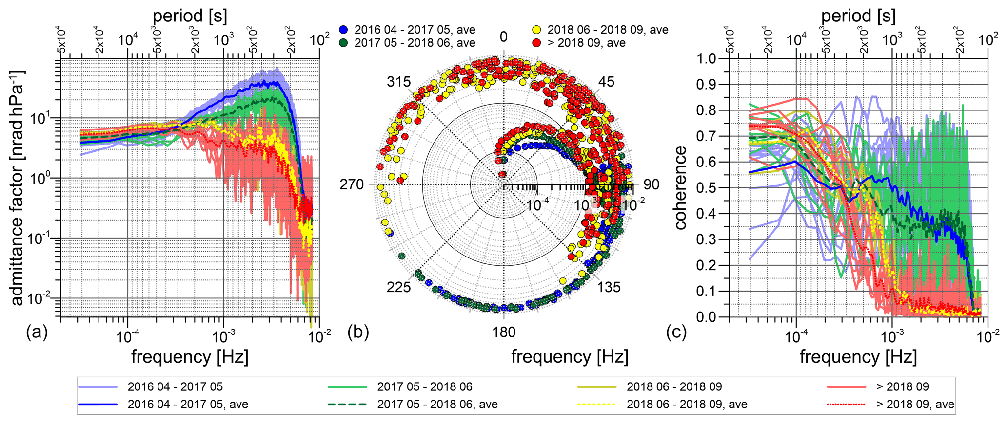
Figure A1Air pressure admittance function of the N–S tilt sensor (LTS) derived from different observation periods covering a period of a few days to less than 3 weeks each. Circles and lines with intense colours show the admittance (a), phase (b) and coherence (c), respectively, averaged over the time series within four intervals (the beginning to May 2017; May 2017–June 2018 (first LTS repair); June–September 2018 (second LTS repair); September 2018 to the end).
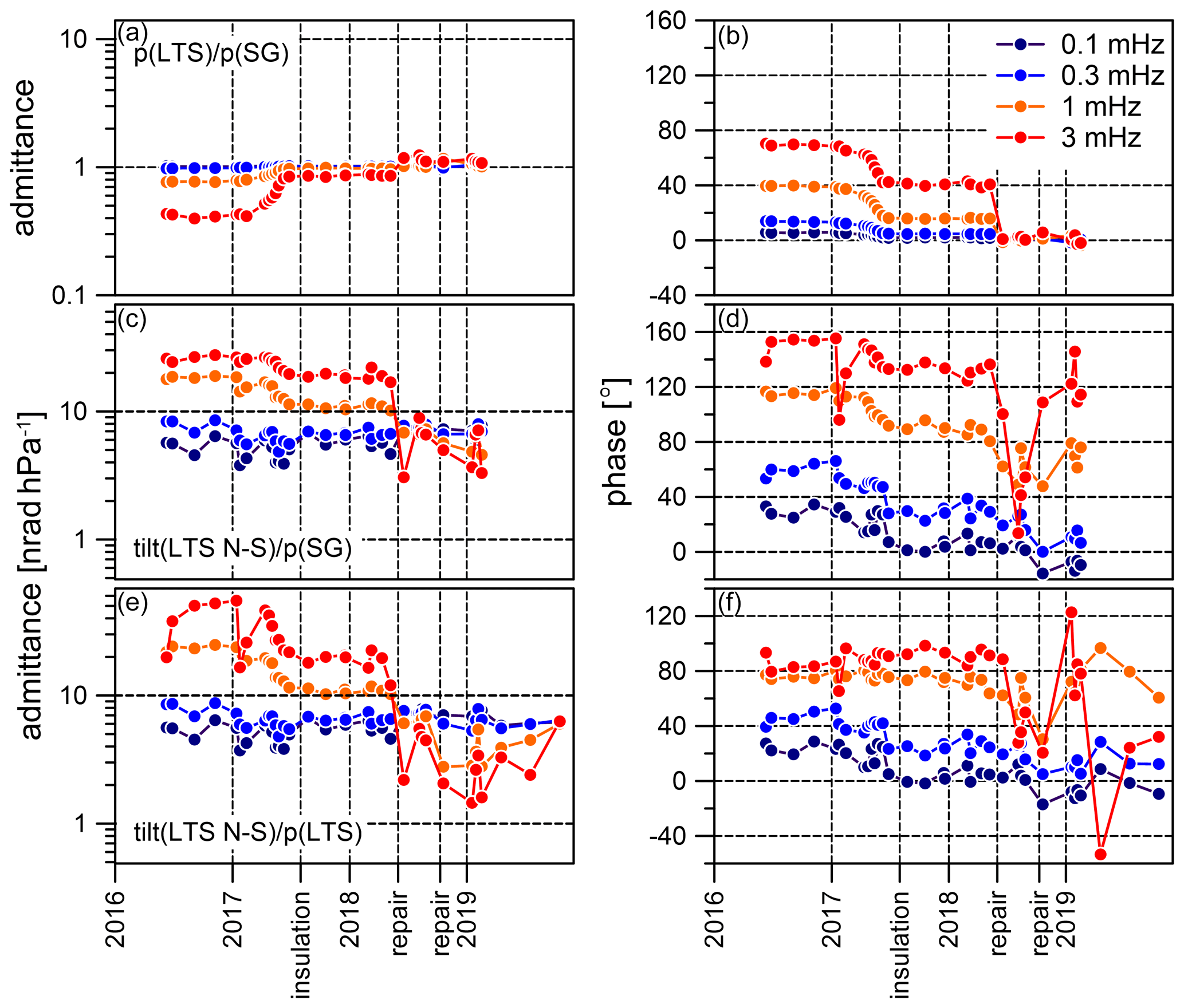
Figure A2Air pressure to tilt (N–S) admittance function and their temporal evolution at selected frequencies derived by using data from different air pressure sensors (e and f – LTS air pressure sensor; c and d – SG air pressure sensor). Panels (a) and (b) show the SG to LTS air pressure admittance function.
ETERNA-x et34-x-v80 software is available at http://ggp.bkg.bund.de/eterna/ (last access: 8 January 2021) (Schüller, 2020). ETERNAv3.4 software is available from the International Center for Earth Tides at https://webdevel.upf.pf/ICET/home.html (last access: 8 January 2021) (Wenzel, 1996). TSoft software is available from the Royal Observatory of Belgium at http://seismologie.oma.be/en/downloads/tsoft (last access: 8 January 2021) (Van Camp and Vauterin, 2005). The gravity data are taken from the International Geodynamics and Earth Tide Service (IGETS) and are available at http://isdc.gfz-potsdam.de/igets-data-base/ (last access: 8 January 2021) (Voigt et al., 2016). The tilt data are available on request from the corresponding author.
GP, JB, HR and RL were responsible for the tiltmeter set-up and maintenance. RL, together with other co-workers, and BM conducted the SG maintenance. The processing of the tilt data was done by GP and JB, while BM processed the gravity data and conducted the tidal analyses and cross-spectral analysis. The final residuals were performed by BM and GP, while the data analyses were conducted by BM, GP and JB. All authors contributed to the interpretation and discussion of the results. BM wrote the paper, with contributions from all co-authors.
The authors declare that they have no conflict of interest.
Both the iWT and the LTS instruments were purchased from the budget dedicated to the development of infrastructure of the Geodetic and Geophysical Institute (GGI), Sopron, Hungary, based on the kind decision of Viktor Wesztergom, the director of GGI.
The great help of ZAMG and its observatory team in providing excellent research facilities is gratefully acknowledged by the authors. The excellent technical support from Frigyes Bánfi, Tibor Molnár and Csaba Molnár (GGI Sopron) is acknowledged too.
We are very grateful to Michel Van Camp and an anonymous reviewer for essential suggestions that helped improve the paper.
Last, but not least, we extend our special thanks to Erich Lippmann for his magnanimous help in the proper maintenance and servicing of his tiltmeter and for his availability for consultation and discussion.
This research has been supported by the NKFIH-OTKA (grant no. K-128527).
This paper was edited by Marnik Vanclooster and reviewed by Michel Van Camp and one anonymous referee.
Agnew, D. C.: Strainmeters and tiltmeters, Rev. Geophys., 24, 579–624, https://doi.org/10.1029/RG024i003p00579, 1986.
Baker, T. F.: Tidal tilt at L1anrwst, north Wales: Tidal loading and earth structure, Geophys. J. R. Astron. Soc., 62, 269–290, https://doi.org/10.1111/j.1365-246X.1980.tb04855.x, 1980.
Baker, T. F. and Lennon, G. W.: Tidal tilt anomalies, Nature, 243, 75–76, https://doi.org/10.1038/243075a0, 1973.
Bendat, J. S. and Piersol, A. G.: Random Data: Analysis and Measurement Procedures, John Wiley and Sons, New York, 602 pp., 2010.
Blaumoser, N.: Hydrological and geological investigations at Trafelberg mountain, Cobs J., 2, 12, 2011.
Bonaccorso, A., Falzone, G., and Gambino, S.: An investigation into shallow borehole tiltmeters, Geophys. Res. Lett., 26, 1637–1640, https://doi.org/10.1029/1999GL900310, 1999.
Bos, M. S. and Scherneck, H. G.: Free ocean tide loading provider, available at: http://holt.oso.chalmers.se/loading/, last access: 21 December 2017.
Boy, J. P., Longuevergne, L., Boudin, F., Jacob, T., Lyard, F., Llubes, M., Florsch, N., and Esnoult, M. F.: Modelling atmospheric and induced non-tidal oceanic loading contributions to surface gravity and tilt measurements, J. Geodyn., 48, 182–188, https://doi.org/10.1016/j.jog.2009.09.022, 2009.
Bryda, G. and Posch-Trözmüller, G.: Geological investigation of the drill core from borehole TB2A: First results, Cobs J., 4, 9, 2016.
Champollion, C., Deville, S., Chéry, J., Doerflinger, E., Le Moigne, N., Bayer, R., Vernant, P., and Mazzilli, N.: Estimating epikarst water storage by time-lapse surface-to-depth gravity measurements, Hydrol. Earth Syst. Sci., 22, 3825–3839, https://doi.org/10.5194/hess-22-3825-2018, 2018.
Cheng, Y. and Andersen, O. B.: Improvement in global ocean tide model in shallow water regions, in: Proceedings of the OSTST Meeting, 18–22 October 2010, Lisbon, Portugal, 2010.
Creutzfeldt, B., Güntner, A., Vorogushyn, S., and Merz, B.: The benefits of gravimeter observations for modeling water storage changes at the field scale, Hydrol. Earth Syst. Sci., 14, 1715–1730, https://doi.org/10.5194/hess-14-1715-2010, 2010.
Crossley, D., Hinderer, J., Casula, G., Francis, O., Hsu, H. T., Imanishi, Y., Jentzsch, G., Kääriänen, J., Merriam, J., Meurers, B., Neumeyer, J., Richter, B., Shibuya, K., Sato, T., and van Dam, T.: Network of Superconducting Gravimeters Benefits a Number of Disciplines, EOS Trans. Am. Geophys. Union, 80, 125–126, https://doi.org/10.1029/99EO00079, 1999.
Crossley, D., Calvo, M., Rosat, S., and Hinderer, J.: More Thoughts on AG–SG Comparisons and SG Scale Factor Determinations, Pure Appl. Geophys., 175, 1699–1725, https://doi.org/10.1007/s00024-018-1834-9, 2018.
Davis, K., Li, Y., and Batzle, M.: Time-lapse gravity monitoring: A systematic 4D approach with application to aquifer storage and recovery, Geophysics, 73, WA61–WA69, https://doi.org/10.1190/1.2987376, 2008.
Dehant, V., Defraigne, P., and Wahr, J. M.: Tides for a convective Earth, J. Geophys. Res., 104, 1035–1058, https://doi.org/10.1029/1998JB900051, 1999.
Deisl, S., Blaumoser, N., and Leonhardt, R.: Hydrology and Geology at the Trafelberg, Cobs Journal, 3, 20, 2014.
Eanes, R. J.: Diurnal and semidiurnal tides from TOPEX/POSEIDON altimetry, EOS Trans. Am. Geophys. Union, 1994 Spring Meeting Supplement, 75, 108, 1994.
Egbert, G. D. and Erofeeva, L.: Efficient inverse modeling of barotropic ocean tides, J. Atmos. Ocean Tech., 19, 183–204, https://doi.org/10.1175/1520-0426(2002)019<0183:EIMOBO>2.0.CO;2, 2002.
Farrell, W. E.: Deformation of the Earth by surface loads, Rev. Geophys., 10, 761–797, https://doi.org/10.1029/RG010i003p00761, 1972.
Fores, B., Champollion, C., Lemoigne, N., and Chéry, J.: Monitoring and modeling of water storage in karstic area (Larzac, France) with a continuous supraconducting gravimeter, in: Geophys. Res. Abstr., EGU2014-4215, EGU General Assembly 2014, 27 April–2 May 2014, Vienna, Austria, 2014.
Fores, B., Champollion, C., Mainsant, G., Albaric, J., and Fort, A.: Monitoring saturation changes with ambient seismic noise and gravimetry in a karst environment, Vadose Zone J., 17, 170163, https://doi.org/10.2136/vzj2017.09.0163, 2018.
Fujimori, K., Ishii, H., Mukai, A., Nakao, S., Matsumoto, S., and Hirata, Y.: Strain and tilt changes measured during a water injection experiment at the Nojima Fault zone, Japan, Island Arc, 10, 228–234, https://doi.org/10.1111/j.1440-1738.2001.00320.x, 2001.
Goodkind, J. M.: The superconducting gravimeter, Rev. Sci. Inst., 70, 4131–4152, https://doi.org/10.1063/1.1150092, 1999.
Güntner, A., Reich, M., Mikolaj, M., Creutzfeldt, B., Schroeder, S., and Wziontek, H.: Landscape-scale water balance monitoring with an iGrav superconducting gravimeter in a field enclosure, Hydrol. Earth Syst. Sci., 21, 3167–3182, https://doi.org/10.5194/hess-21-3167-2017, 2017.
Harrison, J. C.: Cavity and topographic effects in tilt and strain measurements, J. Geophys. Res., 81, 319–328, https://doi.org/10.1029/JB081i002p00319, 1976.
Harrison, J. C.: Implications of cavity, topographic and geological influences on tilt and strain observations, in: Proceedings of the 9th GEOP Conference: An International Symposium on the Application of Geodesy to Geodynamics, Columbus, Ohio, USA, 2–5 October 1978, Dept. of Geodetic Science, Rept. No. 280, 283–287, available at: https://ntrs.nasa.gov/api/citations/19790013330/downloads/19790013330.pdf (last access: 23 November 2020), 1978.
Harrison, J. C. and Herbst, K.: Thermoelastic strains and tilts revised, Geophys. Res. Lett., 4, 535–537, https://doi.org/10.1029/GL004i011p00535, 1977.
Hartmann, H. and Hartmann, W.: Die Höhlen Niederösterreichs, Band 5, Wissenschaftliche Beihefte zur Zeitschrift “Die Höhle”, Landesverein für Höhlenkunde in Wien und Niederösterreich, Vienna, Austria, 54, 616 pp., 2000.
Hector, B., Séguis, L., Hinderer, J., Cohard, J. M., Wubda, M., Descloitres, M., Benarrosh, N., and Boy, J. P.: Water storage changes as a marker for base flow generation processes in a tropical humid basement catchment (Benin): Insights from hybrid gravimetry, Water Resour. Res., 51, 8331–8361, https://doi.org/10.1002/2014WR015773, 2015.
Herbst, K.: Interpretation of Tilt Measurements in the Period Range Above that of the Tides, Terrestrial Sciences Division, Project 7600, Air Force Geophysics Laboratory, 89 pp., available at: https://books.google.at/books?id=vBkotgEACAAJ (last access: 23 November 2020), 1979.
Hinderer, J. and Legros, H.: Elasto-gravitational deformation, relative gravity changes and earth dynamics, Geophys. J. Int., 97, 481–495, https://doi.org/10.1111/j.1365-246X.1989.tb00518.x, 1989.
Hinderer, J., Crossley, D., and Warburton, R.: Superconducting gravimetry, in: Treatise on Geophysics, Volume 3: Geodesy, edited by: Herring, T. and Schubert, G., Elsevier, Amsterdam, the Netherlands, 65–122, 2007.
Jacob, T., Chery, J., Bayer, R., Le Moigne, N., Boy, J. P., Vernant, P., and Boudin, F.: Time-lapse surface to depth gravity measurements on a karst system reveal the dominant role of the epikarst as a water storage entity, Geophys. J. Int., 177, 347–360, https://doi.org/10.1111/j.1365-246X.2009.04118.x, 2009.
Jacob, T., Chéry, J., Boudin, F., and Bayer, R.: Monitoring deformation from hydrologic processes in a karst aquifer using long-baseline tiltmeters, Water Resour. Res., 46, W09542, https://doi.org/10.1029/2009WR008082, 2010.
Jahr, T.: Non-tidal tilt and strain signals recorded at the Geodynamic Observatory Moxa, Thuringia/Germany, Geod. Geodyn., 9, 229–236, https://doi.org/10.1016/j.geog.2017.03.015, 2018.
Jahr, T., Letz, H., and Jentzsch, G.: Monitoring fluid induced deformation of the earth's crust: A large scale experiment at the KTB location/Germany, J. Geodyn., 41, 190–197, https://doi.org/10.1016/j.jog.2005.08.003, 2006a.
Jahr, T., Jentzsch, G., and Gebauer, A.: Observations of fluid induced deformation of the upper crust of the Earth: Investigations about the large scale injection experiment at the KTB site/Germany, Bull. d'Inf. Mar. Terr., 141, 11271–11275, 2006b.
Jahr, T., Jentzsch, G., Gebauer, A., and Lau, T.: Deformation, seismicity, and fluids: Results of the 2004/2005 water injection experiment at the KTB/Germany, J. Geophys. Res., 113, B11410, https://doi.org/10.1029/2008JB005610, 2008.
Jahr, T., Jentzsch, G., and Weise, A.: Natural and man-made induced hydrological signals, detected by high resolution tilt observations at the Geodynamic Observatory Moxa/Germany, J. Geodyn., 48, 126–131, https://doi.org/10.1016/j.jog.2009.09.011, 2009.
Kalmár, J. and Benedek, J.: Determination of water load and catchment lines by the modeling of infiltration and run-off of rain water, Dimenziók: Matematikai Közlemények, 5, 25–29, 2018.
King, G. C. P. and Bilham, R.: Tidal tilt measurement in Europe, Nature, 243, 74–75, https://doi.org/10.1038/243074a0, 1973.
Klügel, T.: Bestimmung lokaler Einflüsse in den Zeitreihen inertialer Rotationssensoren (LOK – ROT), Schlussbericht, DFG-Forschungsprojekt LOK-ROT (SCHR 645/1), Wettzell, available at: https://www.yumpu.com/de/document/view/12632682/lok-rot-geodatisches-observatorium-wettzell (last access: 23 November 2020), 2003.
Kohl, M. L. and Levine, J.: Measurement and interpretation of tidal tilts in a small array, J. Geophys. Res., 100, 3929–3941, https://doi.org/10.1029/94JB02773, 1995.
Krause, P., Naujoks, M., Fink, M., and Kroner, C.: The impact of soil moisture changes on gravity residuals obtained with a superconducting gravimeter, J. Hydrol., 373, 151–163, https://doi.org/10.1016/j.jhydrol.2009.04.019, 2009.
Kümpel, H. J., Varga, P., Lehmann, K., and Mentes, G.: Ground tilt induced by pumping – preliminary results from the Nagycenk test site, Hungary, Acta Geod. Geophys. Hu, 91, 67–78, 1996.
Lampitelli, C. and Francis, O.: Hydrological effects on gravity and correlations between gravitational variations and level of the Alzette River at the station of Walferdange, Luxembourg, J. Geod., 49, 31–38, https://doi.org/10.1016/j.jog.2009.08.003, 2010.
Lesparre, N., Boudin, F., Champollion, C., Chéry, J., Danquigny, C., Seat, H. C., Cattoen, M., Lizion, F., and Longuevergne, L.: New insights on fractures deformation from tiltmeter data measured inside the fontaine de vaucluse karst system, Geophys. J. Int., 208, 1389, https://doi.org/10.1093/gji/ggw446, 2017.
Llubes, M., Florsch, N., Hinderer, J., Longuevergne, L., and Amalvict, M.: Local hydrology, the Global Geodynamics Project and CHAMP/GRACE perspective: some case studies, J. Geodyn., 38, 355–374, https://doi.org/10.1016/j.jog.2004.07.015, 2004.
Longuevergne, L., Boy, J. P., Florsch, N., Viville, D., Ferhat, G., Ulrich, P., Luck, B., and Hinderer, J.: Local and global hydrological contributions to gravity variations observed in Strasbourg, J. Geodyn., 48, 189–194, https://doi.org/10.1016/j.jog.2009.09.008, 2009.
Lyard, F., Lèfevre, F., Letellier, T., and Francis, O.: Modelling the global ocean tides: a modern insight from FES2004, Ocean Dynam., 56, 394–415, https://doi.org/10.1007/s10236-006-0086-x, 2006.
Mangou, S.: Response of tilt and gravity on environmental processes at Conrad observatory, Austria, MSc thesis, University of Vienna, Vienna, 89 pp., 2019.
Mathews, P. M.: Love numbers and gravimetric factor for diurnal tides, in: Proceedings of the 14th International Symposium on Earth Tides, J. Geod. Soc. Jpn., 47, 231–236, https://doi.org/10.11366/sokuchi1954.47.231, 2001.
Matsumoto, K., Takanezawa, T., and Ooe, M.: Ocean tide models developed by assimilating TOPEX/POSEIDON altimeter data into hydrodynamical model: a global model and a regional model around Japan, J. Oceanogr., 56, 567–581, https://doi.org/10.1023/A:1011157212596, 2000.
Meurers, B.: Superconducting Gravimeter Calibration by CoLocated Gravity Observations: Results from GWR C025, Int. J. Geophys., 2012, 954271, https://doi.org/10.1155/2012/954271, 2012.
Meurers, B.: Scintrex CG5 used for superconducting gravimeter calibration, Geod. Geodyn., 9, 197–203, https://doi.org/10.1016/j.geog.2017.02.009, 2018a.
Meurers, B.: 10 years SG gravity time series at Conrad Observatory (Austria) – Station report, in: 1st Workshop on the International Geodynamics and Earth Tide Service (IGETS), 18–20 June 2018, Potsdam, Germany, available at: http://igets.u-strasbg.fr/2018workshop/1.2_03_CO.pdf (last access: 23 November 2020), 2018b.
Meurers, B., Van Camp, M., and Petermans, T.: Correcting superconducting gravity time-series using rainfall modelling at the Vienna and Membach stations and application to Earth tide analysis, J. Geod., 81, 703–712, https://doi.org/10.1007/s00190-007-0137-1, 2007.
Meurers, B., Van Camp, M., Francis, O., and Pálinkáš, V.: Temporal variation of tidal parameters in superconducting gravimeter time-series, Geophys. J. Int., 205, 284–300, https://doi.org/10.1093/gji/ggw017, 2016.
Mikolaj, M. and Meurers, B.: Hydrology Induced Gravity Variation Observed at Vienna and Conrad Observatory, Geophys. Res. Abstr. 15, EGU2013-6003, in: EGU General Assembly 2013, 7–12 April 2013, Vienna, Austria, available at: https://meetingorganizer.copernicus.org/EGU2013/EGU2013-6003.pdf (last access: 23 November 2020), 2013.
Mouyen, M., Longuevergne, L., Chalikakis, K., Mazzilli, N., Ollivier, C., Rosat, S., Hinderer, J., and Champollion, C.: Monitoring of groundwater redistribution in a karst aquifer using a superconducting gravimeter, E3S Web Conf., 88, 2–4, https://doi.org/10.1051/e3sconf/20198803001, 2019.
Papp, G. and Benedek, J.: Numerical modeling of gravitational field lines – the effect of mass attraction on horizontal coordinates, J. Geod., 73, 648–659, https://doi.org/10.1007/s001900050003, 2000.
Papp, G., Ruotsalainen, H., Meurers, B., Leonhardt, R., Benedek, J., Hutchinson, P., and Szántó, M.: Analysis of Environmental and Loading Effects in Tilt and SG Gravity Observations at Conrad (Austria) and Peters Seismological (Australia) Observatories, IUGG-G06l, in: 27th IUGG General Assembly, 8–18 July 2019, Montréal, Québec, Canada, 2019.
Rabbel, W. and Zschau, J.: Static deformations and gravity changes at the earth's surface due to atmospheric loading, J. Geophys., 56, 81–99, 1995.
Ray, R. D.: A global ocean tide Model from TOPEX/POSEIDON Altimetry: GOT99.2, NASA Technical Memorandum 209478, available at: https://ntrs.nasa.gov/api/citations/19990089548/downloads/19990089548.pdf (last access: 23 November 2020), 1999.
Ruotsalainen, H.: Interferometric Water Level Tilt Meter Development in Finland and Comparison with Combined Earth Tide and Ocean Loading Models, Pure Appl. Geophys., 175, 1659–1667, https://doi.org/10.1007/s00024-017-1562-6, 2018.
Ruotsalainen, H., Bán, D., Papp, G., Leonhardt, R., and Benedek, J.: Interferometric Water Level Tilt Meter at the Conrad Observatory, Cobs J., 4, 11, 2016a.
Ruotsalainen, H., Papp, G., Leonhardt, R., Bán, D., Szűcs, E., and Benedek, J.: Comparison of broad band time series recorded by FGI type interferometric water level- and Lippmann's pendulum type tilt meters recording parallel at Conrad observatory, Austria, Geophys. Res. Abstr., 18, EGU2016-6932, in: EGU General Assembly 2016, 17–22 April 2016, Vienna, Austria, 2016b.
Savcenko, R. and Bosch, W.: EOT11a – a new tide model from multimission altimetry, in: Proceedings of the OSTST Meeting, 19–21 October 2011, San Diego, USA, available at: ftp://ftp.sirgas.org/pub/EOT11a/doc/savcenko_eot11a_sandiego.pdf (last access: 23 November 2020), 2011.
Schüller, K.: Program System ETERNA-x et34-x-v80-* for Earth and Ocean Tides Analysis and Prediction, Documentation Manual 01: Theory, January 2020, Surin, Thailand, 209 pp., 2020.
Taguchi, E., Stammer, D., and Zahel, W.: Inferring deep ocean tidal energy dissipation from the global high-resolution data-assimilative HAMTIDE model, J. Geophys. Res.-Oceans, 119, 4573–4592, https://doi.org/10.1002/2013JC009766, 2014.
Tenze, D., Braitenberg, C., and Nagy, I.: Karst deformations due to environmental factors: evidences from the horizontal pendulums of Grotta Gigante, Italy, Boll. Geofis. Teor. Appl., 53, 331–345, https://doi.org/10.4430/bgta0049, 2012.
Van Camp, M. and Francis, O.: Is the instrumental drift of superconducting gravimeters a linear or exponential function of time?, J. Geod., 81, 337–344, https://doi.org/10.1007/s00190-006-0110-4, 2007.
Van Camp, M. and Vauterin, P.: Tsoft: graphical and interactive software for the analysis of time series and Earth tides, Comp. Geosci., 31, 631–640, https://doi.org/10.1016/j.cageo.2004.11.015, 2005.
Van Camp, M., Vanclooster, M., Crommen, O., Petermans, T., Verbeek, K., Meurers, B., van Dam, T., and Dassargues, A.: Hydrological investigations at the Membach station, Belgium, and applications to correct long periodic gravity variations, J. Geophys. Res., 111, BI0403, https://doi.org/10.1029/2006JB004405, 2006.
Van Camp, M., Meurers, B., de Viron, O., and Forbriger, T.: Optimized strategy for the calibration of superconducting gravimeters at the one per mille level, J. Geod., 90, 91–99, https://doi.org/10.1007/s00190-015-0856-7, 2016.
Van Camp, M., de Viron, O., Watlet, A., Meurers, B., Francis, O., and Caudron, C.: Geophysics from terrestrial time-variable gravity measurements, Rev. Geophys., 55, 938–992, https://doi.org/10.1002/2017RG000566, 2017.
Voigt, C., Förste, C., Wziontek, H., Crossley, D., Meurers, B., Pálinkáš, V., Hinderer, J., Boy, J. P., Barriot, J. P., and Sun, H.: Report on the Data Base of the International Geodynamics and Earth Tide Service (IGETS), Scientific Technical Report STR – Data 16/08, GFZ German Research Centre for Geosciences, Potsdam, https://doi.org/10.2312/GFZ.b103-16087, 2016.
Watlet, A., Kaufmann, O., Triantafyllou, A., Poulain, A., Chambers, J. E., Meldrum, P. I., Wilkinson, P. B., Hallet, V., Quinif, Y., Van Ruymbeke, M., and Van Camp, M.: Imaging groundwater infiltration dynamics in the karst vadose zone with long-term ERT monitoring, Hydrol. Earth Syst. Sci., 22, 1563–1592, https://doi.org/10.5194/hess-22-1563-2018, 2018.
Watlet, A., Van Camp, M., Francis, O., Poulain, A., Rochez, G., Hallet, V., Quinif, Y., and Kaufmann, O.: Gravity monitoring of underground flash flood events to study their impact on groundwater recharge and the distribution of karst voids, Water Resour. Res., 56, e2019WR026673, https://doi.org/10.1029/2019WR026673, 2020.
Weise, A.: Neigungsmessungen in der Geodynamik – Ergebnisse von der 3-Komponentenstation Metsahovi, PhD Thesis, Technical University of Clausthal, Clausthal, Germany, 180 pp., 1992.
Weise, A., Jentzsch, G., Kiviniemi, A., and Kääriäinen, J.: Comparison of long period tilt measurements: Results from two clinometric stations Metsähovi and Lohja, Finland, J. Geodyn., 27, 237–257, https://doi.org/10.1016/S0264-3707(97)00067-7, 1999.
Wenzel, H. G.: The Nanogal Software: Earth Tide Data Processing Package ETERNA 3.30, Bull. d'Inf. Mar. Terr., 124, 9425–9439, 1996.
Zürn, W.: Simplistic models of vertical seismic noise above 0.1 mHz derived from local atmospheric pressure, Bull. d'Inf. Mar. Terr., 137, 10867–10874, 2002.
- Abstract
- Introduction
- Observation site and instrumentation
- Gravity and tilt preprocessing and determination of residuals
- Local tide models and air pressure admittance
- Gravity and tilt residuals at Conrad Observatory
- Discussion
- Conclusion
- Appendix A: Analysis of the air pressure admittance function for tilt
- Code and data availability
- Author contributions
- Competing interests
- Acknowledgements
- Financial support
- Review statement
- References