the Creative Commons Attribution 4.0 License.
the Creative Commons Attribution 4.0 License.
 | 16 Dec 2020
Flexible vector-based spatial configurations in land models
Shervan Gharari
Martyn P. Clark
Naoki Mizukami
Wouter J. M. Knoben
Jefferson S. Wong
Alain Pietroniro
Land models are increasingly used in terrestrial hydrology due to their process-oriented representation of water and energy fluxes. A priori specification of the grid size of the land models is typically defined based on the spatial resolution of forcing data, the modeling objectives, the available geospatial information, and computational resources. The variability of the inputs, soil types, vegetation covers, and forcing is masked or aggregated based on the a priori grid size. In this study, we propose an alternative vector-based implementation to directly configure a land model using unique combinations of land cover types, soil types, and other desired geographical features that have hydrological significance, such as elevation zone, slope, and aspect. The main contributions of this paper are to (1) implement the vector-based spatial configuration using the Variable Infiltration Capacity (VIC) model; (2) illustrate how the spatial configuration of the model affects simulations of basin-average quantities (i.e., streamflow) as well as the spatial variability of internal processes (snow water equivalent, SWE, and evapotranspiration, ET); and (3) describe the work and challenges ahead to improve the spatial structure of land models. Our results show that a model configuration with a lower number of computational units, once calibrated, may have similar accuracy to model configurations with more computational units. However, the different calibrated parameter sets produce a range of, sometimes contradicting, internal states and fluxes. To better address the shortcomings of the current generation of land models, we encourage the land model community to adopt flexible spatial configurations to improve model representations of fluxes and states at the scale of interest.


Land models have evolved considerably over the past few decades. Initially, land models (or land-surface models) were developed to provide the lower boundary conditions for atmospheric models (Manabe, 1969). Since then land models have increased in complexity, and they now include a variety of hydrological, biogeophysical, and biogeochemical processes (Pitman, 2003). Including this broad suite of terrestrial processes in land models enables simulations of energy and water fluxes and carbon and nitrogen cycles.
Despite the recent advancements in process representation in land models, there is currently limited understanding of the appropriate spatial complexity that is justified based on the available data and the purpose of the modeling exercise (Hrachowitz and Clark, 2017). The increase of computational power, along with the existence of more accurate digital elevation models and land cover maps, encourages modelers to configure their models at the finest spatial resolution possible. Such hyper-resolution implementation of land models (Wood et al., 2011) can provide detailed simulations at spatial scales as small as a 1 km2 grid over large geographical domains (e.g., Maxwell et al., 2015). However, the computational expense of hyper-resolution models could potentially be reduced using more creative spatial discretization strategies (Clark et al., 2017).
It is common to adopt concepts of hydrological similarity to reduce computational costs. In this approach, spatial units are defined based on similarity in geospatial data, under the assumption that processes, and therefore parameters, are similar for areas within a spatial unit (e.g., Vivoni et al., 2004; Newman et al., 2014). Hydrological response units (HRUs) are perhaps the most well-known technique to group geospatial attributes in hydrological models. HRUs can be built based on various geospatial characteristics; for example, Kirkby and Weyman (1974), Knudsen et al. (1986), Flügel (1995), Winter (2001), and Savenije (2010) all have proposed to use geospatial indices to discretize a catchment into hydrological units with distinct hydrological behavior. HRUs can be built based on soil type such as proposed by Park and Van De Giesen (2004). HRUs can also be built based on fieldwork and expert knowledge (Naef et al., 2002; Uhlenbrook et al., 2004), although the spatial domain of such classification will be limited to the catchment of interest and the spatial extent of the field measurements. HRUs are often constructed by GIS-based overlaying of maps of different characteristics and can have various shapes such as non-regular (sub-basins), grid, hexagon, or triangulated irregular network, also known as TIN (Beven, 2011; Marsh et al., 2012; Olivera et al., 2006). Land models are also beginning to adopt concepts of hydrological similarity (e.g., Newman et al., 2014; Chaney et al., 2018). Traditionally land models use the tiling scheme, whereby a grid box is subdivided into several tiles of unique land cover, each described as a percentage of the grid (Koster and Suarez, 1992). Similarly, the concept of grouped response units (GRUs; Kouwen et al., 1993) assumes similar hydrological property for areas with identical soil, vegetation, and topography. The GRU concept is utilized in the MESH land modeling framework (Pietroniro et al., 2007).
A long-standing challenge is understanding the impact of grid size on model simulations (Wood et al., 1988). The effect of model grid size can have a significant impact on model simulation across scale, especially if the model parameters are linked to characteristics which are averaged out across scale (Blöschl et al., 1995). Shrestha et al. (2015) have investigated the performance of the Community Land Model (CLM) v4.0 coupled with ParFlow across various grid sizes. They concluded that grid sizes of more than 100 m can significantly affect the sensible heat and latent heat fluxes as well as soil moisture. Also using the CLM, Singh et al. (2015) demonstrated that topography has a substantial impact on model simulations at the hillslope scale (∼100 m), as aggregating the topographical data changes the runoff generation mechanisms. This is understandable as the CLM is based on a topographic wetness index (Beven and Kirkby, 1979; Niu et al., 2005). However, Melsen et al. (2016) evaluated the transferability of parameter sets across the temporal and spatial resolutions for the Variable Infiltration Capacity (VIC) model implemented in an Alpine region. They concluded that parameter sets are more transferable across various grid sizes in comparison with parameter transferability across different temporal resolutions. Haddeland et al. (2002) showed that the transpiration from the VIC model highly depends on grid resolution. It remains debatable how model parameters and performance can vary across various grid resolutions (Liang et al., 2004; Troy et al., 2008; Samaniego et al., 2017).
The representation of spatial heterogeneity is an ongoing debate in the land modeling community (Clark et al., 2015). The key issue is to define which processes are represented explicitly and which processes are parameterized. The effect of spatial scale on emergent behavior has been studied for catchment-scale models – the concepts of representative elementary area (REAs) and representative elementary watershed (REW) were introduced to study the effect of spatial aggregation on system-scale emergent behavior (Wood et al., 1988; Reggiani et al., 1999). The effect of scale on model simulations is not well explored for land models. More work is needed to understand the extent to which the heterogeneity of process representations is sufficient for the purpose of a given modeling application and the extent to which the existing data can support the model configurations (Wood et al., 2011; Beven et al., 2015) and guarantee a fidelius model.
In this study, we configure the VIC model in a flexible vector-based framework to understand how model simulations depend on the spatial configuration. The remainder of this paper is organized as follows: in Sect. 2, we present the concept of vector-based configuration for land models. In Sect. 3 we describe the study area and the data sets used in this study as well as the design of the experiments and elaborate the VIC model and mizuRoute as the vector-based routing model. In Sect. 4 we describe the results of the experiments. Section 5 discusses the implication of spatial discretization strategies for large-scale land model applications. The paper ends in Sect. 6 with conclusions of this study and implications for future work.
Land models are often applied at a regularly spaced grid. Land models are typically set up at a range of spatial configurations, ranging from grid sizes of 0.02 to 2∘ (approximately 2 to 200 km) and applied at sub-daily temporal resolutions for the simulation of energy fluxes. A priori specification of the grid size of the land models is often derived from forcing resolutions, modeling objectives, available geospatial data, and computational resources and is usually based on modeling convenience. Figure 1e–h illustrate the typical land model configuration – here the modeler selects a cell size, and then the soil, vegetation, and forcing files are all aggregated or disaggregated to the target cell size. Original data resolution and spatial distribution of soil, land cover, and forcing data are smeared while upscaled to the resolution of interest. Any change in the modeling resolution will require upscaling or downscaling of the geophysical data set once again.
In this study, we configure the land models using non-regular shapes. Figure 1a–d present an example of non-regular shapes created through spatial intersections of the land covers and soil type shapes. These vector-based configurations of the geospatial data are then forced at the original meteorological forcing resolution or its upscaled or downscaled values, resulting in computational units. Therefore, each computational unit has unique geospatial data such as soil, vegetation, slope, and aspect and is forced with a unique forcing. In this configuration, changing meteorological forcing resolution does not affect the decisions needed to upscale the geospatial data such as soil type and land cover to the grid resolution.
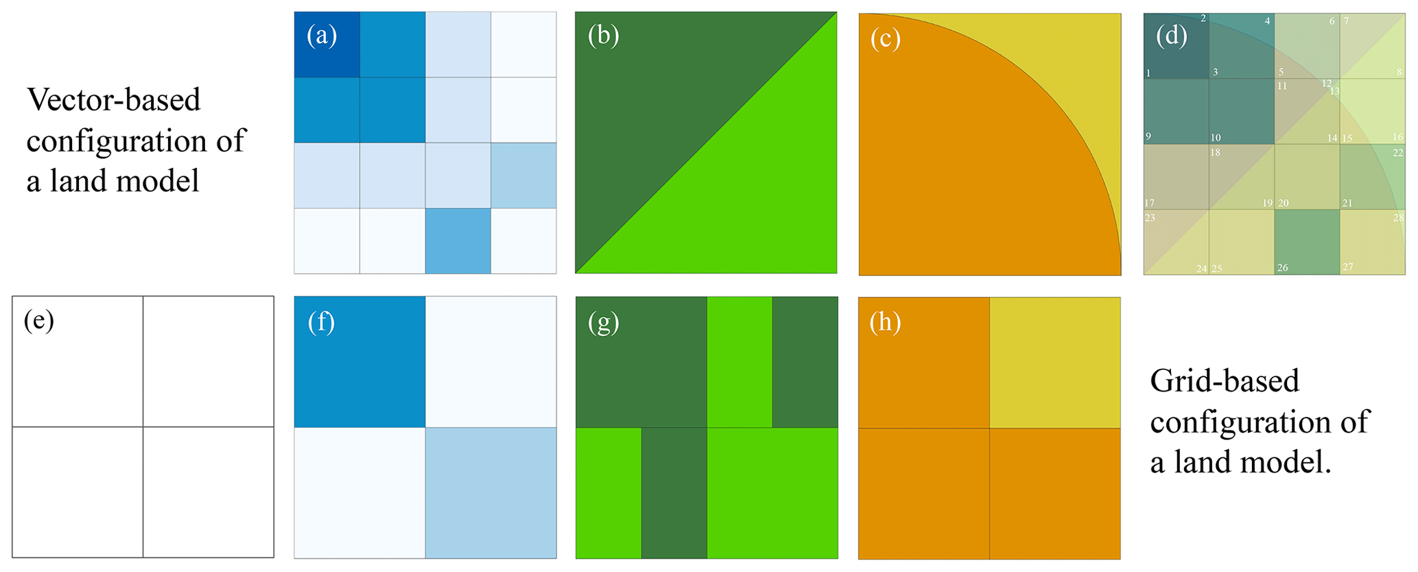
Figure 1Panels (a–d) indicate vector-based configuration of a land model. (a) Meteorological forcing at its original resolution or upscaled and downscaled resolutions, (b) land covers, (c) soil types with their spatial extent, and (d) vector-based configuration with 28 computational units each with unique forcing, soil type, and land cover type. The bottom row indicates typical grid-based configuration of a land model; (e) a priori resolution should be decided; (f) meteorological forcing should be upscaled or downscaled to the grid resolution; (g) land cover percentage should be calculated for each modeling grid, or a dominate land cover should be selected to represent that grid; and finally (h) soil characteristics for each modeling grid should be identified.
The benefits of vector-based configuration of land models can be summarized as follows:
-
There is no need for a priori assumption on modeling grid size. In traditional land model implementation, the modeler selects a grid resolution (which is often a regular latitude/longitude grid). The soil parameters and forcing data from any resolution must be aggregated, disaggregated, resampled, or interpolated for every grid size. The land cover data are often only considered as a percentage for every grid, and spatial location of the land cover is lost. However, in the vector-based setup, these decisions are only based on the input and forcing data that are chosen to be used in the modeling practice, and no upscaling or downscaling to grid size is needed. Furthermore, the size of computational units can vary across the modeling domain depending on the variability of the meteorological forcing and geospatial heterogeneity. For example, the spatial density of computational units can be higher in mountainous areas, where temperature and precipitation gradients are larger while avoiding an unnecessarily high number of computational units in areas with a lower gradient in meteorological forcing.
-
There is a reasonable relation between available meteorological forcing and geospatial data resolution and the number of computational units. Computational units that are the result of available geophysical data sets forced with the original forcing data logically represent the maximum number of computational units that can be hydrologically unique. A higher number of computational units than the proposed setup will arguably provide an unnecessary computational burden due to identical forcing data and geospatial information.
-
Direct simplification of geospatial data is possible. The vector-based implementation facilitates easier aggregation of computational units. It is easier to aggregate similar soil types or similar forested areas into unified shapes with a basic GIS function (dissolving for example) than this would be if all data had to be upscaled or downscaled into a different grid size.
-
Direct specification of physical parameters is possible, and unrealistic combinations of land cover, soil, and other geophysical information are avoided. As each computational unit has a specific type of land cover, soil type, and other physical characteristics, it is straightforward to specify parameter values based on lookup tables (i.e., no averaging; upscaling is needed). This is favorable because the modeler does not need to make decisions about methods used for upscaling of geophysical data at the grid level. Also, this might avoid the unrealistic combination of parameter sets that might be considered by the model at a grid scale, such as equiprobable combination of land cover on soil type which may not exist in reality, which will be increasing the fidelity of the model representation of the processes (we will elaborate this further in the context of the VIC model in the Discussion). We emphasize that the ease of parameter allocation for vector-based implementation of land models does not address the challenge of finding the right parameter sets for each computational unit.
-
It has the ability to compare and constrain the parameter values for computational units and their simulations. The impact of land cover, soil type and elevation zone can be evaluated separately. For example, the vector-based implementation makes it easier to test if forested areas generate less surface runoff than grasslands. This might be more challenging at the gird-based configuration, in which there are a combination of different land cover types at grid scale. Similarly, the vector-based implementation may simplify regularization efforts across large geographical domains. These relative constraints can be utilized to translate often patchy expert knowledge into a sophisticated land model.
-
It is possible to incorporate additional data. If needed, additional data, such as slope and aspect, for example, can be incorporated in building the computational units, accounting for changes in shortwave radiation or lapse rates for temperature. The changes can be implemented outside of the model in the forcing files. Computational units can be built also based on variation of the leaf area index (LAI), giving an additional layer of information in addition to the land cover type. The additional information can be easily ingested into the model without extra effort in contrast to changing the model parameter files at the grid scale.
-
Comparison of model simulations and in situ point-scale observation and visualization are easier. The vector-based implementation of land models makes it easier to compare the point measurement to model simulation as the model simulations preserve the extent of geospatial features.
-
The selection of models is modular and controlled. The vector-based implementation identifies the characteristics and spatial boundary of geospatial domains. A model might not be suitable for processes of some of the geospatial domains. Alternatively, processes of a computational unit that is beyond the capacity of one model can be replaced with an alternative model. For example, computational units that are glaciered can be replaced with more suitable models, while the spatial configuration and forcings remain identical. Consequently, the effect of features such as glaciers can be better studied as more expert models can be applied to glaciers, while the rest of the computational units can be simulated with a model that includes general processes.
3.1 Study area
Experiments are performed for the Bow River at Banff, as part of the Saskatchewan River basin, with an area of approximately 2210 km2, located in the Canadian Rockies, province of Alberta, Canada. Most of the Bow River streamflow is due to snowmelt (nivo-glacial regime). The average basin elevation is 2130 m, ranging from 3420 m at the peak top to 1380 m above mean sea level at the outlet (town of Banff). The basin annual precipitation is approximately 1000 mm, with a range of 500 mm for the Bow Valley up to 2000 mm for the mountain peaks. The predominant land cover is conifer forest in the Bow Valley and rocks and gravels for mountain peaks above the treeline.
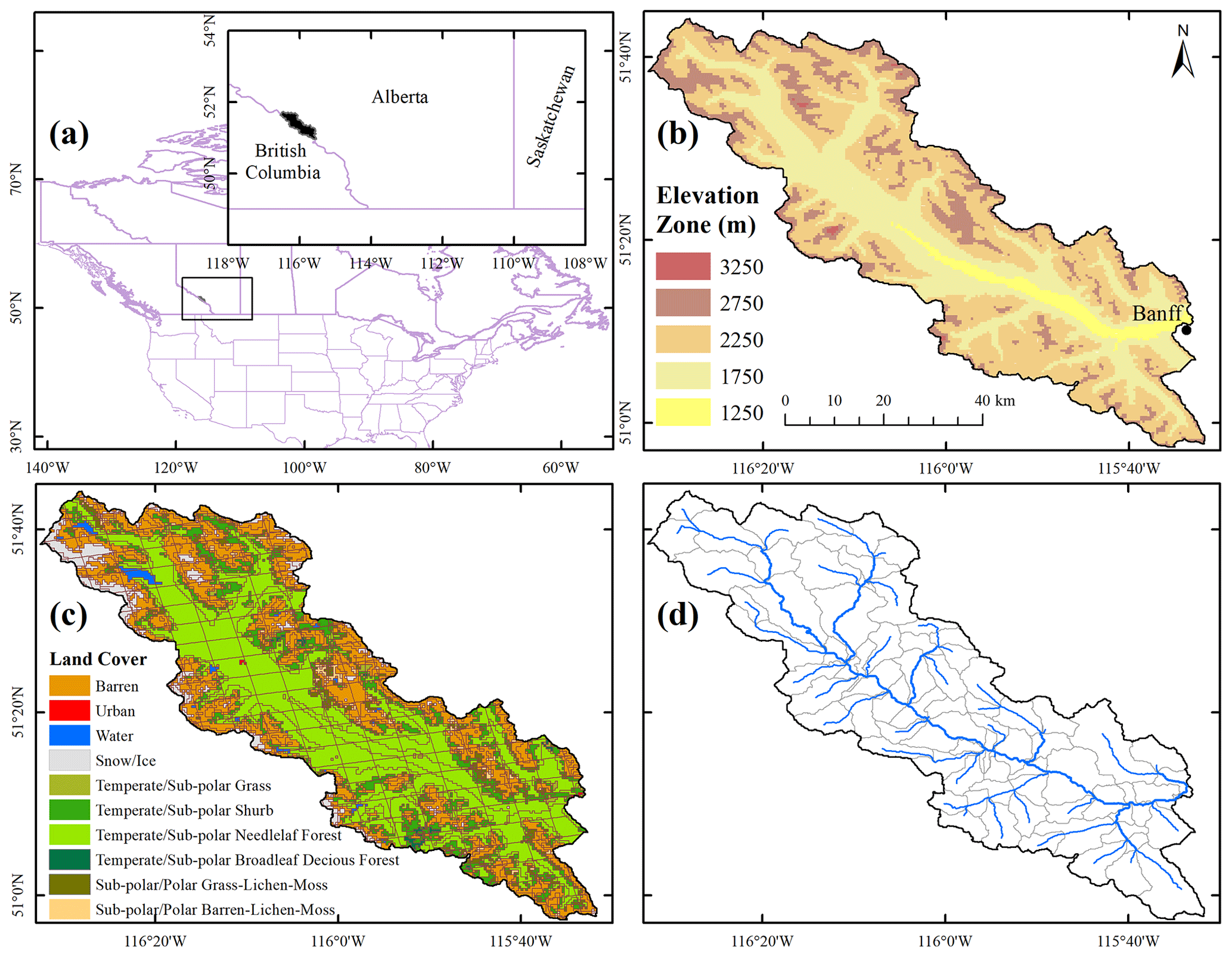
Figure 2(a) The location of the Bow River basin at Banff, (b) Bow River basin elevation, (c) computational units for geospatial data of elevation zones, land cover, and soil type forced at WRF original resolution at 4 km (Case 3–4 km), and (d) river network topology and associated sub-basins that are used for the vector-based routing.
3.2 Geospatial data and meteorological forcing
3.2.1 Model input data set and forcing
The inputs and forcing we used to set up the model are as follows:
-
Land cover: we used the land cover map NALCMS-2005 v2 (North American Land Change Monitoring System; Latifovic et al., 2004) that is produced by CEC (Commission for Environmental Cooperation). NALCMS-2005 v2 includes 19 different classes. The land cover map is used to set up the vegetation file and vegetation library (lookup table) for the VIC model (Nijssen et al., 2001).
-
Soil texture: we used the Harmonized World Soil Data (HWSD; Fischer et al., 2008). For each polygon of the world harmonized soil we use the highest proportion of soil type. The HWSD provide the information for two soil layers; in this study we base our analyses on the lower soil layer reported in HWSD to define the soil characteristics needed for the VIC soil file.
-
Digital elevation model: in this study we make use of existing hydrologically conditioned digital elevation models (DEMs) to (1) derive the river network topology for the vector-based routing, mizuRoute; and (2) derive the slope, aspect, and elevation zones, which are used to estimate the forcing variables. For the first purpose we use the hydrologically conditioned DEM of HydroSHED (Lehner et al., 2006) with a resolution of 3 arcsec, approximately 90 m; for the second purpose, we use the HydroSHED 15 arcsec DEM (approximately 500 m).
-
Meteorological forcing: we used the weather research and forecasting (WRF) model simulation for the continental United States, with a temporal resolution of 1 h and spatial resolution of 4 km (Rasmussen and Liu, 2017). For upscaling the WRF input forcing, we use the CANDEX package (https://doi.org/10.5281/zenodo.2628351) to map the seven forcing variables to various resolutions (1∕16, 1∕8, 1∕4, 1∕2, 1, and 2∘ from the original resolution of 4 km). We used the required variables from the WRF data set, namely, total precipitation, temperature, short- and longwave radiation at the ground surface, V and U components of wind speed, and water vapor mixing ratio.
The shortwave radiation is rescaled based on the slope and aspect of the respective computational unit (refer to Appendix A for more details). In this study we differentiated four aspects and five slope classes. The temperatures at 2 m are adjusted using the environmental lapse rate of −6.5 ∘C for an 1000 m increase in elevation. The assumed lapse rate aligns with earlier findings from the region of study (Pigeon and Jiskoot, 2008).
3.2.2 Observed data for model calibration
The daily streamflow is extracted from the HYDAT (WSC, Water Survey of Canada) for Bow at Banff with a gauge ID of 05BB001. These data are used for parameter calibration and identification of the VIC parameters.
3.3 Land model and routing scheme
3.3.1 The Variable Infiltration Capacity (VIC) model
The VIC model was developed as a simple land-surface/hydrological model (Liang et al., 1994) that has been applied worldwide (Melsen et al., 2016). In this study we use the classic VIC version 5. The VIC model combines sub-grid probability distributions to simulate surface hydrology such as variable infiltration capacity formulation (Zhao et al., 1980). The VIC model uses three soil layers to represent the subsurface. While each soil layer can have various physical soil parameters (e.g., saturated hydraulic conductivity and bulk density), each layer is assumed to be uniform across the entire grid, regardless of the vegetation type variability in that grid. The VIC model assumes a tile vegetation implementation within each grid similar to the mosaic approach of Koster and Suarez (1992) with biophysical formulations for transpiration (Jarvis, 1976). To account for spatial variability in vegetation, the VIC model allows for root depths to be adjusted for every vegetation type. The vegetation parameters (e.g., stomatal resistance, LAI, albedo) are often identical for each land cover type across the modeling domain. The VIC model can account for different elevation zones to account for the temperature lapse rate, given the elevation difference in a grid cell, and also for the distribution of precipitation over the identified elevation zones.
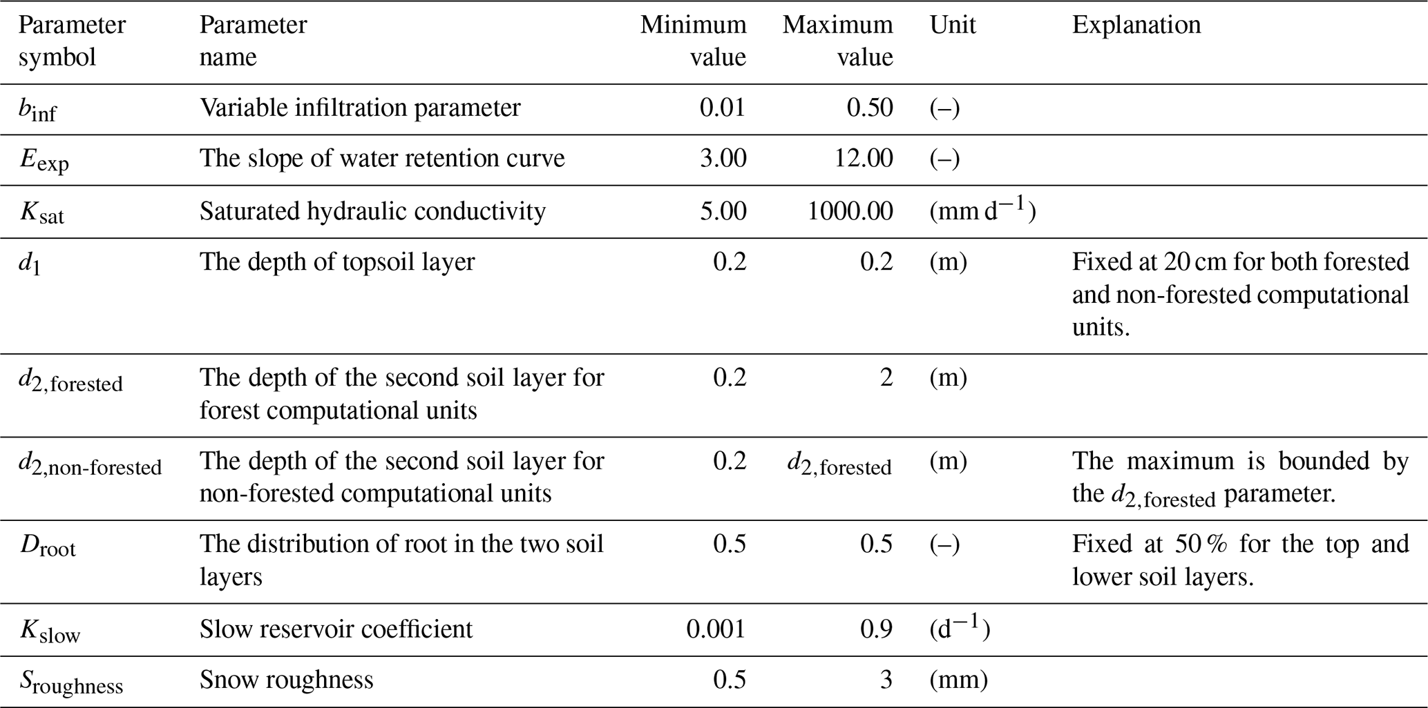
In the experiments for this study, we calibrate a subset of VIC parameters namely binf, Eexp, Ksat, d2,forested, d2,non-forested, Kslow, and Sroughness (names are mentioned in Table 1). Following the concept of GRUs (Kouwen et al., 1993), we assume that the computational units with similar geophysical characteristics (soil and land cover) possess similar parameter values. We make sure that the d2,forested is larger than the d2,non-forested as the root depths are deeper for forested regions (constraining relative parameters). For the sake of simplicity, we limit the root zone to the upper soil layers and replace the five-parameter VIC baseflow1 with a linear reservoir (refer to Gharari et al., 2019, for further explanation). We also assume that the two top soil layers possess homogeneous soil characteristics.
3.3.2 mizuRoute, a vector-based routing scheme
In this study, we make use of the vector-based routing model mizuRoute (Mizukami et al., 2016). Vector-based routing models can be configured for different computational units than the land model uses (e.g., configuring routing models using sub-basins derived from existing hydrologically conditioned DEMs such as HydroSHEDS, Lehner et al., 2006, or MERIT Hydro, Yamazaki et al., 2019). This removes the dependency of the routing on the grid size or computational unit configurations and eliminates the decisions that are often made to represent routing-related parameters at grid scale. Therefore, we can ensure that two model configurations with different geospatial configurations are routed using the same routing configuration. The intersection between the computational units in the land model and the sub-basins in the routing model defines the contribution of each computational units from the land model to each river segment.
The impulse response function (IRF) routing method (Mizukami et al., 2016) is used for this study. IRF, which is derived based on diffusive wave equation, includes two parameters – wave velocity and diffusivity. The diffusive wave parameters are set to 1 m s−1 and 1000 m2 s−1 respectively and remain identical for all the river segments. The river network topology, assuming approximately a 25 km2 starting threshold for the sub-basin size, is based on a 92-segment river network, depicted in Fig. 3d.
Table 1The VIC model parameters that are subject to perturbation for model calibration for the designed experiments.
3.4 Experimental design
In this study, we configure the VIC model in a flexible vector-based framework to understand how model simulations depend on the spatial configuration. We consider four different methods to discretize the landscape for seven different spatial forcing grids (see Table 2). The landscape discretization methods include (1) simplified land cover and soils; (2) full detail on land cover and soils; (3) full detail on land cover and soils, including elevation zones; and (4) full detail on land cover and soils, including elevation zones, slope, and aspect. The different spatial forcing resolutions are 4 km, 0.0625, 0.125, 0.25, 0.5, 1, and 2∘. This design enables us to separate discretization of the landscape based on geospatial data from the spatial resolution of the forcing data.
Table 2The numbers of computational units for the Bow River at Banff, given different spatial discretization of land cover, soil type, elevation zones, slopes, and aspects forced with various forcing resolutions.

3.4.1 Experiment 1: how does the spatial configuration affect model performance?
As the first experiment, we focus on how well the various configurations simulate observed streamflow for Bow River at Banff. We calibrate the parameters for the different configurations in Table 2. Model calibration is accomplished using the Genetic Algorithm implemented in the OSTRICH framework (Mattot, 2005; Yoon and Shoemaker, 2001), maximizing the Nash–Sutcliffe efficiency (ENS; Nash and Sutcliffe, 1970) using a total budget of 1000 model evaluations given the available resources limited by the most computationally expensive model (Case 4–4 km).
3.4.2 Experiment 2: how well do calibrated parameter sets transfer across different model configurations?
As the second experiment, we focus on how various configurations can reproduce the result from the configuration with highest computational units for a given parameter set. In other words, this experiment evaluates accuracy–efficiency trade-offs – i.e., the extent to which spatial simplifications affect model performance under the assumption that similar computational units possess identical parameters across various configurations. This is important as it enables modelers to understand accuracy–efficiency trade-offs, given the available data and the purpose of the modeling application. This experiment is based on perfect model experiments using the model with the highest computational unit as a synthetic case (Case 4–4 km). Synthetic streamflow for every river segment is generated using a calibrated parameter set for Case 4–4 km. The models with a lower number of computational units are then simulated using the exact same parameter set used for generating the synthetic streamflow. The differences in streamflow simulation, quantified using ENS, provide an understanding of how the simulations deteriorate when the spatial and forcing heterogeneities are masked or upscaled. This also will bring an understanding on how sensitive the changes are along the river network and at the gauge location at which the models are calibrated against the observed streamflow data. Similarly, we compare the spatial patterns of snow water equivalent for the different spatial configurations.
4.1 Experiment 1
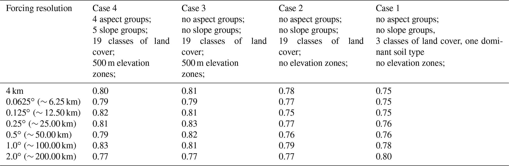
The various model configurations are compared with respect to the Nash–Sutcliffe performance metric (ENS). Results show that all the models, including the ones that are configured with coarser resolution forcings, can simulate streamflow with ENS as high as 0.70 (Table 3). It is noteworthy to mention that the configuration of Case 4–1∘ has a higher ENS value compared to the cases with highest computational units, Case 4–4 km for example. This might be due to various reasons including (1) compensation of forcing aggregation on possible forcing bias at finer resolution and (2) compensation of forcing aggregation on model states and fluxes and possible adjustment for model structural inadequacy and hence directing the optimization algorithm to different possible solutions across configurations.
Table 3The highest calibrated Nash–Sutcliffe performance metric (ENS) for the different model configurations. Details on the geospatial cases are provided in Table 2.
We use a single objective calibration algorithm for model calibration, however, and for investigating the parameter uncertainty, we check the behavioral parameter sets with ENS higher than 0.7 (arbitrary units). These parameter sets indicate very different soil characteristics. Figure 3a illustrates the possible combinations of behavioral parameter sets for Case 2–4 km (ENS > 0.7). As a specific example, saturated hydraulic conductivity, Ksat, and slope of water retention curve, Eexp, have very different combinations of values within the specified parameter ranges for calibration. The result indicates the two parameters that are often fixed or a priori allocated based on lookup tables can exhibit significant uncertainty and non-identifiability. It is also noteworthy to mention that among the parameters, Kslow seems to be the most identifiable parameter, while it is set to the upper limit range. There might be two explanations for this behavior: (1) this might be related to the nivo-glacier regime of the study basin, which has a strong yearly cycle due to snow accumulation and snowmelt; (2) the lack of macropore water movement to the baseflow component results in dampened input to this component and in return results in Kslow being higher than expected for a baseflow reservoir (for further reading, refer to Gharari et al., 2019). Overall, the results indicate that calibrating the VIC model parameters using a sum of squared objective function at the basin outlet does not constrain the VIC subsurface parameters. Additionally, we examine the difference between the fluxes, in this case transpiration, for all the parameter sets presented in Fig. 3a. Figure 3b illustrates differences between the yearly transpiration flux for the computational units of case 2–4 km. This difference can be as high as 250 mm yr−1 indicating the internal uncertainty of fluxes and related states in reproducing similar performance metric. This difference can be the basis of model diagnosis to understand which computational units are causing the internal uncertainty and perhaps the underlying reasons for it.
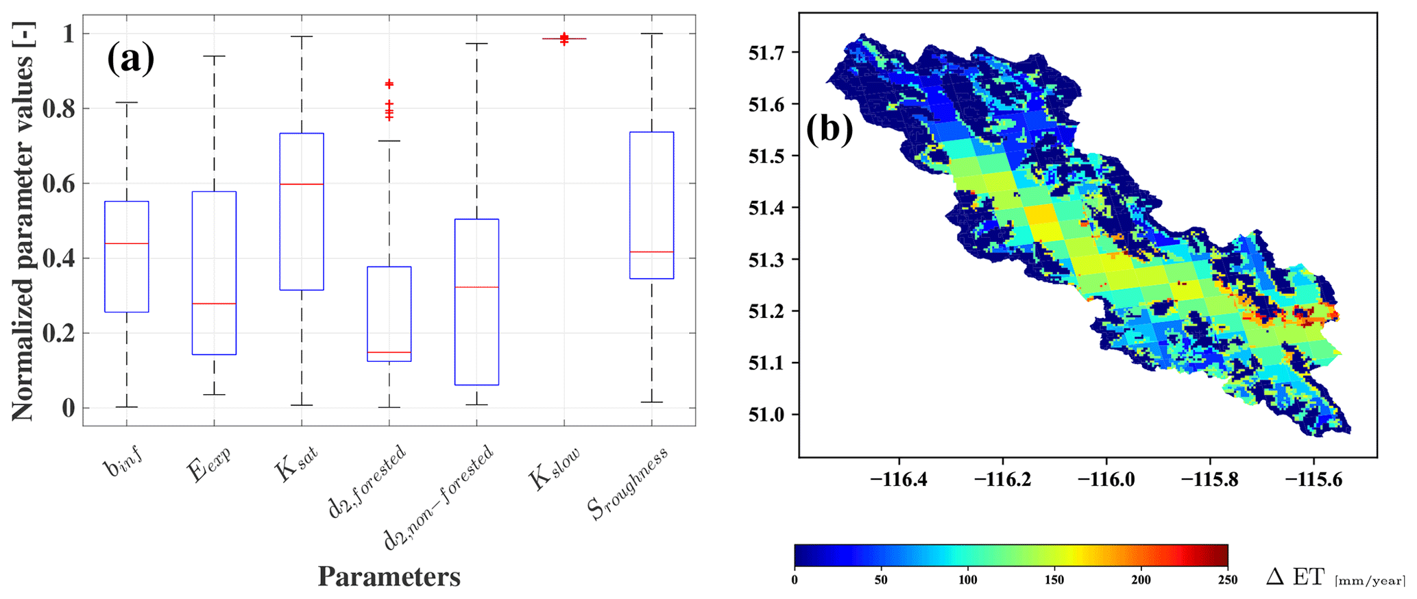
Figure 3(a) The normalized values for the parameters of Case 2–4 km that have ENS (Nash–Sutcliffe efficiency) values of higher than 0.7. (b) The difference of largest and smallest yearly simulated transpiration for parameter sets with ENS above 0.7.
4.2 Experiment 2
The second experiment compares the performance of a parameter set from the Case 4–4 km across the configurations with degraded geophysical information and aggregated spatial information. Here we choose a parameter set that has ENS of above 0.7 (this can be any other parameter sets). Figure 4 shows the evaluation metric, ENS, for the streamflow of every river segment across the domain in comparison with the synthetic case (Case 4–4 km). From Fig. 4, it is clear that the ENS is less sensitive for river segments with a larger upstream area (i.e., segments that are located more downstream). This result has two major interpretations (i) the parameter transferability across various configurations is dependent on the sensitivity of simulation at the scale of interest, meaning that as long as good performance is achieved in the context of modeling, for example for the streamflow at the basin outlet, the parameters can be said to transferable for that scale; and (ii) often inferred parameters at larger scale may not guarantee good performing parameters at the smaller scales (read upstream areas) as the change in the performance metric varies significantly across scale for the smaller modeling elements.
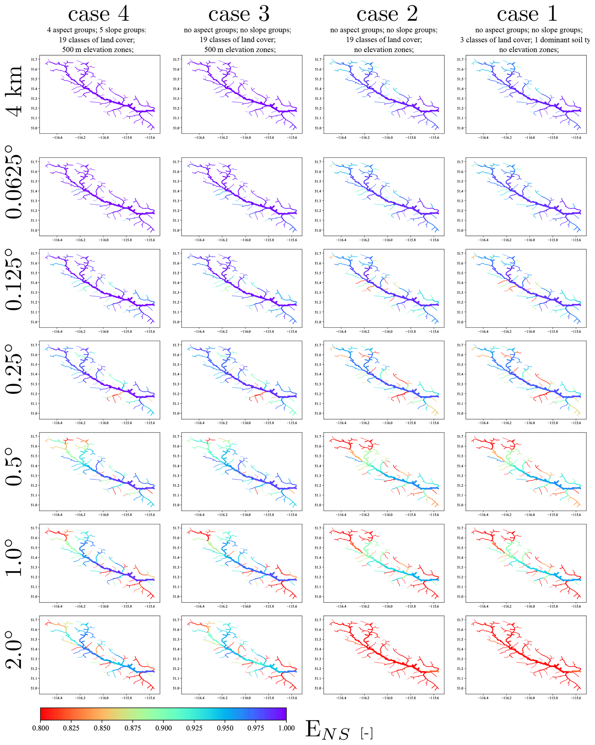
Figure 4Differences of the simulated streamflow at river segments in comparison with the synthetic case, Case 4–4 km, expressed in the performance metric ENS.
To understand the spatial patterns of model simulations for all the configurations, we evaluate the distribution of the snow water equivalent, SWE, for the computational units on 5 May 2004 (Fig. 5). In general, the SWE follows the forcing resolution and its aggregation. Although coarser forcing resolution results in coarser SWE simulation, the geospatial details such as elevation zones, slopes, and aspects result in more realistic representation of SWE as the snow layer is thinner for south-facing slopes where more melt can be expected to occur and thicker for higher elevation zones (compare SWE simulations for Case 4–2∘ and Case 3–2∘ in Fig. 5), which is consistent with higher precipitation volumes and slower melt at higher elevation. Another observation from Fig. 5 is the unrealistic distribution of SWE for configurations without elevation zones (Case 2 and Case 1). The lack of elevation zones results in both valley bottoms and mountaintops being forced with the same temperature. Snow is more durable in the forested areas, which are at lower elevation, as the result of the model formulation, while SWE is less for higher mountains, which is unrealistic. We remind the reader that the various spatial patterns of SWE across different configurations are from the simulations that result in a rather similar performance metric, ENS, for the streamflow at the outlet of the basin.
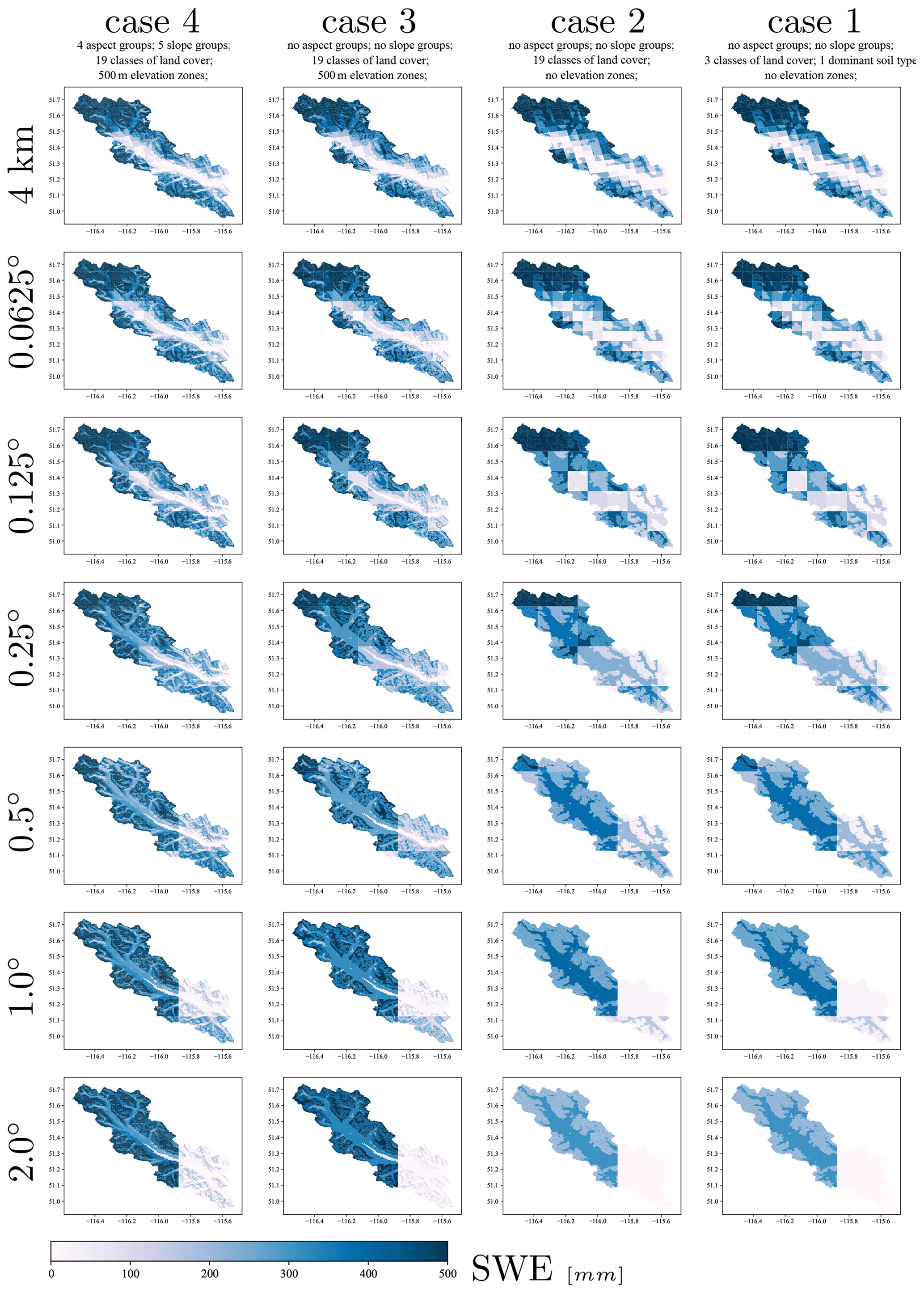
Figure 5Comparison of the snow water equivalent for 5 May 2004 for various configurations.
Figure 6a shows the performance of the streamflow across various configurations for the most downstream river segment (the gauged river segment which is used for parameter inference through calibration). Figure 6a illustrates that most of the configurations have a similar scaled ENS at the basin outlet. We compared the maximum snow water equivalent across different configurations for a computational unit located in the Bow Valley bottom (an arbitrary location of −116.134∘ W and 51.382∘ E) for the year 2004 (Fig. 6b). The result indicates that the SWE is higher for configurations with coarser forcing resolutions (almost triple). This is due to the reduced temperature as a result of masking warmer valley bottom by cooler and higher forcing grids over the Rockies. Such analyses can provide insights into the appropriate model configurations for different applications. Also, and as an example, if model configurations of different complexity are known to show similar performance for a given parameter set, uncertainty and sensitivity analysis can be done initially on the models with fewer computational units, and the results of the analysis can be applied to models with a higher number of computational units. This analysis can be repeated for different parameter sets, e.g., poorly performing parameter sets or randomly selected parameter sets, to better understand accuracy–efficiency trade-offs of the model within its specified parameters ranges.
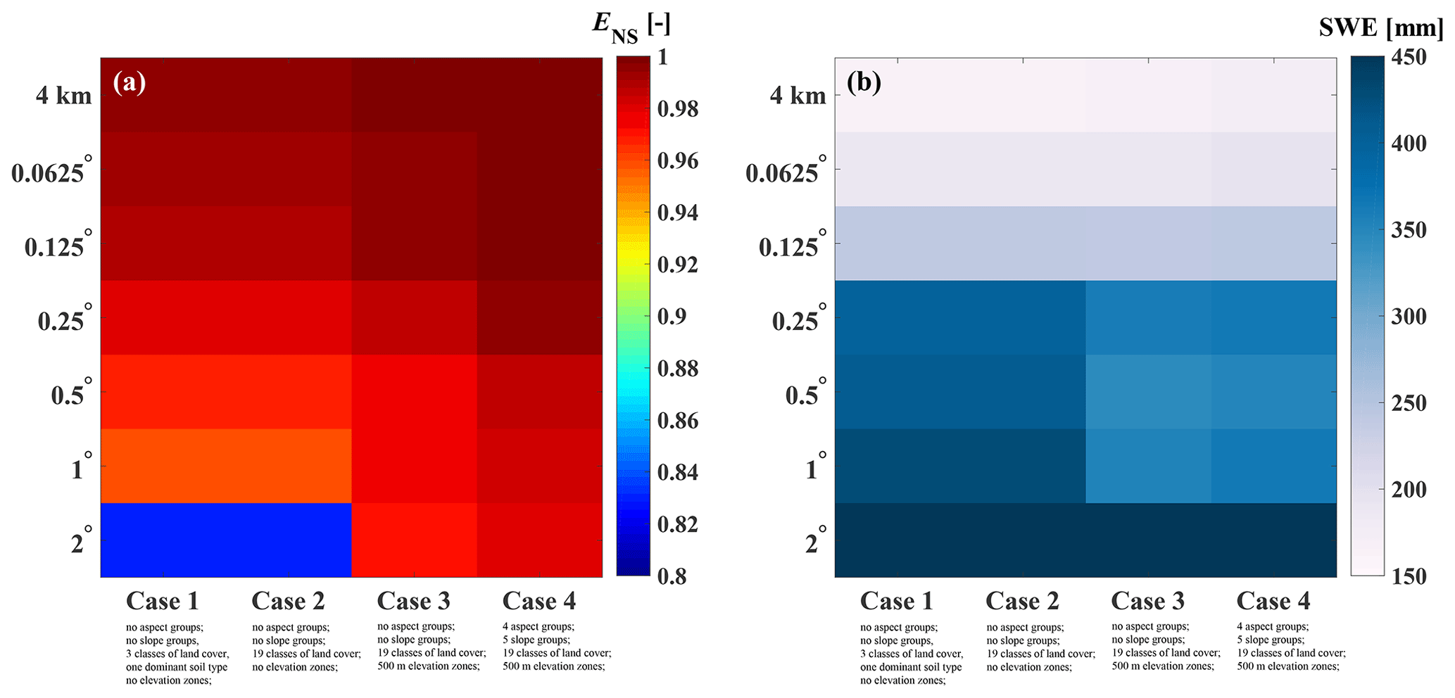
Figure 6(a) The relative performance of model simulation across various configurations with a single parameter set. (b) Maximum of snow water equivalent for an arbitrary location of −116.134∘ W and 51.382∘ E located in Bow Valley bottom across various model configurations for the year 2004.
In this study, we proposed a vector-based configuration for land models and applied this setup to the VIC model. We used a vector-based routing scheme, mizuRoute, which was forced using output from the land model (one-way coupling). Unlike the grid-based approach, there is no upscaling of land cover percentage or soil characteristics to a new grid size. This enables us to separate the effects of changes in forcing resolution from changes in the spatial configurations. As mentioned earlier in Sect. 2, the vector-based configuration of land models may help to avoid unrealistic configuration of soil type, land cover, or elevation zones that may happen in traditional grid-based implementation and hence increase the model fidelity. As an example, VIC configuration at grid scale assumes equal distribution of land cover over different elevation zones. Figure 7b illustrates how the traditional VIC configuration at grid scale wrongly considers forested land cover above the treeline. This issue is avoided in the vector-based configuration as the setup will only include two computational units of forested area below the treeline and bare soil above the treeline (Fig. 7a). The vector-based setup provides more flexibility in comparing the model simulations across computational units (as an example, refer to Fig. 5) and also comparing model simulations with point measurements, such as snow water equivalent. Moreover, the vector-based routing results in complete decoupling of the land model computational units' spatial extent from routing sub-basins. For the grid-based configuration of land models, it is often the case that in land, model grids and routing grids are identical, which result in further decisions on upscaling of the routing direction to the land model grid scale.

Figure 7(a) The realistic configuration of a natural system with land cover consisting of 50 % bare soil and 50 % forest within a grid located in two different elevation zones above and below the treeline which is preserved with vector-based configurations and (b) the traditional VIC configurations for the given system at the grid for the two elevation zones and two land cover types which results in an unrealistic combination of forested land cover above the treeline and bare soil below the treeline.
Our results illustrate that various vector-based spatial configuration of the VIC model generates similar large-scale simulations of streamflow when the setups are calibrated by maximizing the Nash–Sutcliffe score at the basin outlet. Similarly, we have shown that often behavioral parameter sets yield similar ENS values and can be significantly uncertain (Fig. 3a) or have significant differences for their internal behavior, which may be very well masked by aggregation of the result at the grid scale or basin scale (Figs. 3b and 5). Generally, parameter, state and flux uncertainties are not often evaluated or reported on in land models (Demaria et al., 2007) or are ignored by tying parameters, linking specific hydraulic conductivity to the slope of the water retention curve, for example, so that the possible combinations of parameters are reduced. Moreover, the behavior of the Kslow parameter can be revealing of the VIC model structural deficiencies, which are not often explored for land models. The recession coefficient obtained from recession analysis on the observed hydrograph is approximately 0.01 d−1, while the calibrated Kslow has much higher values of around 0.90 d−1. This can be due to a dampened response from the two top soil layers and a lack of macropore water movement to the baseflow component. Similarly, and due to a lack of macropore water movement in the VIC model, and land models in general, it is impossible to infer the Kslow based on recession analysis on the observed hydrograph (for further reading on this and also recession analysis refer to Gharari et al., 2019). This finding can be generalized to the five-parameter VIC baseflow, highlighting the need to properly evaluate the often not observable but calibrated baseflow parameters for the VIC model and if it is possible to identify five parameters based on the recession limps of a hydrograph.
Land models are often applied at large spatial scales. The results clearly show that the deviation of streamflow is much lower in river segments with a larger upstream area (Figs. 4 and 6a). It is often the case that the model parameters and associated processes are inferred through calibration on the streamflow at the basin outlet or over a large contributing area. We argue that this may not be a valid strategy for process understanding at the smaller scale (read computational units), given the large uncertainty exhibited by the parameters. Therefore, hyper-resolution modeling efforts (Wood et al., 2011) may suffer from poor process representation and parameter identification at the scale of interest (Beven et al., 2015). What is needed instead of efficiency metrics that aggregate model behavior across both space (e.g., at the outlet of the larger catchment) and time (e.g., expressing the mismatch between observations and simulations across the entire observation period as a single number) is diagnostic evaluation of the model's process fidelity at the scale at which simulations are generated in the case of available observations (e.g., Gupta et al., 2008; Clark et al., 2016).
One might argue that the spatial discretization is important for the realism of model fluxes and states. Moving to a significantly high number of computational units may result in computational units that are similar in their forcing and geospatial fabric (such as soil and land cover types). Based on the result of this study for snow water equivalent (Fig. 5), we can argue that the snow patterns are fairly similar for the configurations that have elevation zones and finer resolution of forcing (Cases 3 and 4 and forcing resolution less than 0.125∘). (, in which m is the model, x and θ are model forcing and the model parameter set, and and are upscaled forcing and parameter values at coarser spatial representation.)
The analysis of the accuracy–efficiency trade-off presented in this study, Fig. 6, can be used in model analysis such as sensitivity and uncertainty. One can assume that a configuration with fewer computational units can be a surrogate for a model with more computational units, under the condition that both models are known to behave similarly for a given parameter set. The calibration can be done on the model configuration with fewer computational units, and the parameters can be transferred directly to the model with more computational units or can be used as an initial point for optimization algorithm to speed up the calibration process. Similarly, the sensitivity analyses can be done primarily on the model with fewer computational units.
In this study, and following the concept hydrological similarity, we assume the parameters of computational units are identical for computational units with similar soil and land cover. The degree of validity of hydrological similarity concepts is debatable. For example, at the catchment scale, Oudin et al. (2010) have shown that the overlap between catchments with similar physiographic attributes and catchments with similar model performance for a given parameter set is only 60 %. Thus, physiographic similarity (in our case expressed through GRUs) does not necessarily imply similarity of hydrologic behavior, even though this is the critical assumption underlying GRUs. The VIC parameters can be linked to many more characteristics such as slope, height above nearest drainage (HAND; Renno et al., 2008; Gharari et al., 2011), or topographic wetness index (Beven and Kirkby, 1979), as has been done by Mizukami et al. (2016) and Chaney et al. (2018). Techniques such as multiscale parameter regionalization (MPR; Samaniego et al., 2010) can be used to scale parameter values for different model configurations. However, the functions that are used to link computational units and physical attributes to model parameters remain mostly based on inference, (i.e., calibration), and the reproducibility of those relationships are not very well explored. However, application of these techniques, such as in this case that has significant parameter and process uncertainty and significant accuracy–efficiency trade-off, should be put through rigorous tests (Merz et al., 2020; Liu et al., 2016).
A key outstanding challenge is for models to provide the right results for the right reasons (Kirchner, 2006). Thoughtful strategies to formulate parameter and process constraints based on expert knowledge can reduce the plausible range of behavioral parameter sets. In this study, we imposed a simple parameter constraint that the root zone moisture storage of forested area should be larger than the non-forested area (Table 1). Additional process constraints, if available, can be increasingly difficult to satisfy. More rigorous parameter estimation methods that satisfy the fidelity constraints based on expert knowledge are required (e.g., Gharari et al., 2014).
In this study, the vector-based routing configuration does not include lakes and reservoirs. This is often a neglected element of land modeling efforts and has only attracted limited attention compared to the its impact on terrestrial water cycle (Haddeland et al., 2006; Yassin et al., 2019). The presence of lakes and reservoirs and their interconnections reduces the, already limited, ability of inference of land model parameters based on calibration on the observed streamflow (Dang et al., 2020).
Although not primarily the result of this study, however, the nivo-glacial regime of the Bow River basins is mostly dominated by snowmelt that contributes mostly to streamflow through baseflow (slow component of the hydrograph). The high Nash–Sutcliffe efficiency, ENS, is partly due to the fact that it is rather easy for the land model to capture the yearly cycle of the streamflow only with snow processes (see, e.g., Knoben et al., 2020, demonstrating this for the Kling–Gupta efficiency), while rapid subsurface water movement, such as macropore movement, is largely missing in the land models (Gharari et al., 2019). Therefore, more caution is needed for the calibration of land model parameters for flood forecasting (Vionnet et al., 2020) for the Bow region and all the nivo-glacial river systems in western Canada, McKenzie, Yukon, and Colombia River basins.
The vector-based configuration of land models can provide modelers with more flexibility, e.g., representing the impact of various forcing resolutions or geospatial data representation. The conclusions from this study can be summarized as follows:
-
The land model configuration with the highest number of computational units may not result in improved performance and better spatial simulation, in terms of obtained efficiency scores, while the internal model state and fluxes can show significant uncertainty.
-
There is significant parameter and structural uncertainty associated with the land model (in this case, the VIC model). This uncertainty poses challenges for the process and parameter inference when the model is calibrated by minimizing the sum of squared differences between simulated and observed streamflow. Any parameter regionalization efforts should take these uncertainties into account. Our results emphasize that more attention is needed on the topic of parameter and process inference at finer modeling scales.
-
A model configuration with lower computational units, coarser resolution, and less geospatial information may reproduce model simulations with similar efficiency scores as configurations with higher computational units. Less computationally expensive configurations can be used for primary uncertainty and sensitivity analysis.
A key scientific challenge is hydrological scaling; i.e., how do small-scale heterogeneities shape large-scale fluxes? Addressing this challenge requires a mix of both explicit representations of spatial heterogeneity (enabled through spatial discretization of the landscape) and implicit representations of heterogeneity (enabled through sub-grid parameterizations). The contribution in this paper is to advance flexible spatial configurations for land models – our approach improves the explicit representation of spatial heterogeneities, at least compared to traditional approaches that simply drape a grid over the landscape. Much more work is required across all spatial scales to carefully evaluate how a mix of explicit and implicit representations of spatial heterogeneity can improve process representations. We encourage the community to develop tools which can enable easier and more flexible configuration of land models that can be used to explore the above-mentioned research questions.
This appendix reflects on the method and equations that have been used to calculate the ratio of the solar radiation on a surface with slope and aspect to a flat surface. Please note that the angles in the equations are in radians, but for better communication we express angles in degrees in the text.
Declination angle: the declination angle can be calculated for each day of year and is the same for the entire Earth (Sarbu and Sebarchievici, 2017):
in which δ is the declination angle in radians, and d is the number of days in a year starting from 1 January.
Hour angle: the hour angle is the angle expressed at the solar hour. The reference of solar hour angle is solar noon (hour angle is set to zero) when the sun is passing the meridian of the observer or when the solar azimuth is 180∘ (north direction with azimuth of 0∘). The hour angle can be calculated based on the
in which α, ϕ, and δ are the altitude angle, latitude of the observer, and declination angle. The sunset and sunrise hour can be calculated as (when sun is at horizon and solar altitude angle is zero)
More caution is needed using Eq. (A3) for latitudes above and below 66.55∘ north and south respectively where it can be always day or night with no sunrise or sunset during part of the year. The number of daylight hours that can be split before and after the solar noon equally can be calculated based on (assuming 15∘ for every 1 h)
And therefore, the hour angle can be easily calculated for the time before and after solar noon (every 15∘ is equal to an hour). The hour angle is negative for the time before solar noon and positive for the time after solar noon. Note the solar noon does not often coincide with 12:00 of the local time zone. There are relationships to find the local time of solar noon.
Solar altitude angle: the solar altitude angle is the angle of sun rays with the horizontal plane of an observer. This angle is maximum at solar noon and 0∘ for sunset and sunrise. The altitude angle can be calculated based on the
For the solar noon, when ω, the hour angle, is zero, the question simplifies to
Solar azimuth: the solar azimuth angle, ASun, reflects the angle of the sun on the sky from the north in a clockwise fashion. The azimuth angle can be calculated as
The solar azimuth angle for the solar noon is set to be 180∘.
Surface azimuth (a.k.a. aspect): the surface azimuth angle, ASurface, reflects the direction of any tilted surface to a northern direction. This azimuth is fixed for any point, while the solar azimuth changes over hours and seasons.
Angle of incidence θ: this angle represents the angle between sun rays and the normal vector of a sloped surface. The model angle of the incidence for a slope surface, β, and aspect of ASurface over latitudes of ∅ can be calculated as (Kalogirou, 2009; in the reference formulation the azimuth is from the south, which is corrected here for north)
For the flat surface, both ASurface and β are set to 0∘. The incident angle can be calculated for the flat surface as
In the case that the angle of incident is larger than 90∘, the surface shades itself.
Correction of shortwave radiation based on slope and aspect: in this study we correct the WRF shortwave radiation based on the surface slope and aspect. We first back-calculated the incoming shortwave radiation by dividing the shortwave radiation provided by the cosine of the incident angle of the flat surface. Then we can calculate the solar radiation of the sloped surface. multiplying this value by the cosine of the incident angle of the slope surface. Basically, this ratio is
The effect of the atmosphere is considered in the WRF product itself. However, and for incident levels close to 90∘, the ratio, R, might have very high values, which results in the surface receiving an unrealistically high value of radiation, even higher than the solar constant, 1366 W m−2, at the top of the atmosphere. For cases with cosine values of the incident angle lower than 0.05, we set the ratio to 0 to avoid this unrealistic condition.
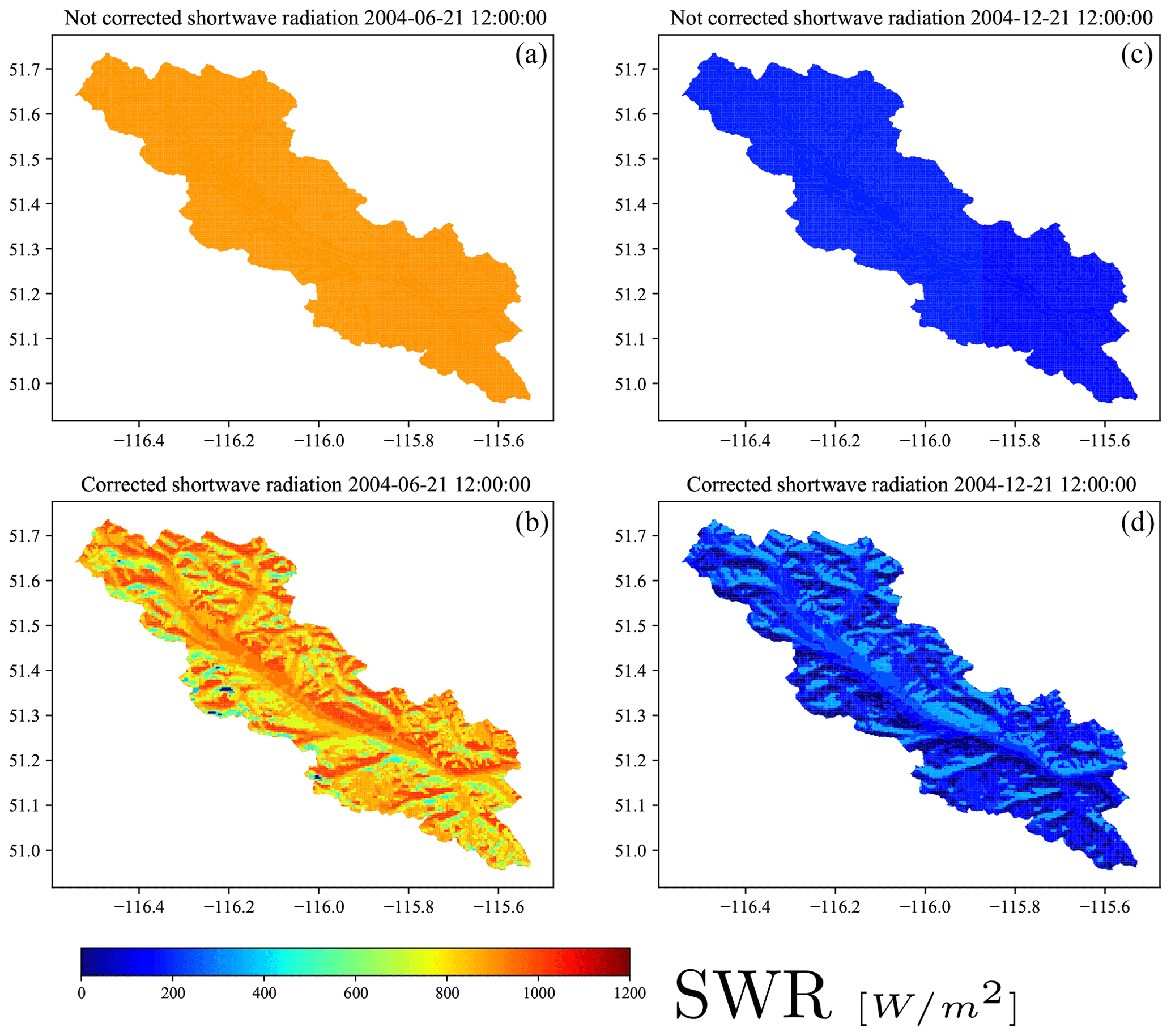
Figure A1Shortwave radiation (a) not corrected for slope and aspect and (b) corrected for slope and aspect for 21 June 2020 and (c) not corrected for slope and aspect and (d) corrected for slope and aspect for 21 December 2020.
All the data used in this study are available publicly (refer to references).
SG, AP, and MPC developed the concept. SG did the model setup and simulations. SG and MC wrote the paper. WJMK, NM, and JSW contributed to the writing and editing of the paper, scientific comments, interpretation of results, and preparation of figures.
The authors declare that they have no conflict of interest.
This research was carried out by the Global Water Futures (GWF) core modeling team.
This paper was edited by Niko Wanders and reviewed by two anonymous referees.
Beven, K. J.: Rainfall-runoff modelling: the primer, John Wiley and Sons, 2011.
Beven, K. J. and Kirkby, M. J.: A physically based, variable contributing area model of basin hydrology/Un modèle à base physique de zone d'appel variable de l'hydrologie du bassin versant, Hydrolog. Sci. J., 24, 43–69, 1979.
Beven, K. J., Cloke, H., Pappenberger, F., Lamb, R., and Hunter, N.: Hyperresolution information and hyperresolution ignorance in modelling the hydrology of the land surface, Sci. China Earth Sci., 58, 25–35, https://doi.org/10.1007/s11430-014-5003-4, 2015.
Blöschl, G., Grayson, R. B., and Sivapalan, M.: On the representative elementary area (REA) concept and its utility for distributed rainfall-runoff modelling, Hydrol. Process., 9, 313–330, 1995.
Chaney, N. W., Van Huijgevoort, M. H. J., Shevliakova, E., Malyshev, S., Milly, P. C. D., Gauthier, P. P. G., and Sulman, B. N.: Harnessing big data to rethink land heterogeneity in Earth system models, Hydrol. Earth Syst. Sci., 22, 3311–3330, https://doi.org/10.5194/hess-22-3311-2018, 2018.
Clark, M. P., Nijssen, B., Lundquist, J. D., Kavetski, D., Rupp, D. E., Woods, R. A., Freer, J. E., Gutmann, E. D., Wood, A. W., Brekke, L. D., Arnold, J. R., Gochis, D. J., and Rasmussen, R. M.: A unified approach for process‐based hydrologic modeling: 1. Modeling concept, Water Resour. Res., 51, 2498–2514, https://doi.org/10.1002/2015WR017198, 2015.
Clark, M. P., Schaefli, B., Schymanski, S. J., Samaniego, L., Luce, C. H., Jackson, B. M., Freer, J. E., Arnold, J. R., Moore, R. D., Istanbulluoglu, E., and Ceola, S.: Improving the theoretical underpinnings of process‐based hydrologic models, Water Resour. Res., 52, 2350–2365, https://doi.org/10.1002/2015WR017910, 2016.
Clark, M. P., Bierkens, M. F. P., Samaniego, L., Woods, R. A., Uijlenhoet, R., Bennett, K. E., Pauwels, V. R. N., Cai, X., Wood, A. W., and Peters-Lidard, C. D.: The evolution of process-based hydrologic models: historical challenges and the collective quest for physical realism, Hydrol. Earth Syst. Sci., 21, 3427–3440, https://doi.org/10.5194/hess-21-3427-2017, 2017.
Dang, T. D., Chowdhury, A. F. M. K., and Galelli, S.: On the representation of water reservoir storage and operations in large-scale hydrological models: implications on model parameterization and climate change impact assessments, Hydrol. Earth Syst. Sci., 24, 397–416, https://doi.org/10.5194/hess-24-397-2020, 2020.
Demaria, E. M., Nijssen, B., and Wagener, T.: Monte Carlo sensitivity analysis of land surface parameters using the Variable Infiltration Capacity model, J. Geophys. Res.-Atmos., 112, D11113, https://doi.org/10.1029/2006JD007534, 2007.
Fischer, G., Nachtergaele, F., Prieler, S., van Velthuizen, H. T., Verelst, L., and Wiberg, D.: Global Agro-ecological Zones Assessment for Agriculture (GAEZ 2008), IIASA, Laxenburg, Austria and FAO, Rome, Italy, 2008.
Flügel, W. A.: Delineating hydrological response units by geographical information system analyses for regional hydrological modelling using PRMS/MMS in the drainage basin of the River Bröl, Germany, Hydrol. Process., 9, 423–436, 1995.
Gharari, S., Hrachowitz, M., Fenicia, F., and Savenije, H. H. G.: Hydrological landscape classification: investigating the performance of HAND based landscape classifications in a central European meso-scale catchment, Hydrol. Earth Syst. Sci., 15, 3275–3291, https://doi.org/10.5194/hess-15-3275-2011, 2011.
Gharari, S., Hrachowitz, M., Fenicia, F., Gao, H., and Savenije, H. H. G.: Using expert knowledge to increase realism in environmental system models can dramatically reduce the need for calibration, Hydrol. Earth Syst. Sci., 18, 4839–4859, https://doi.org/10.5194/hess-18-4839-2014, 2014.
Gharari, S., Clark, M., Mizukami, N., Wong, J. S., Pietroniro, A., and Wheater, H.: Improving the representation of subsurface water movement in land models, J. Hydrometeorol., 2401–2418, https://doi.org/10.1175/JHM-D-19-0108.1, 2019.
Gupta, H. V., Wagener, T., and Liu, Y.: Reconciling theory with observations: elements of a diagnostic approach to model evaluation, Hydrol. Process., 22, 3802–3813, https://doi.org/10.1002/hyp.6989, 2008.
Haddeland, I., Matheussen, B. V., and Lettenmaier, D. P.: Influence of spatial resolution on simulated streamflow in a macroscale hydrologic model, Water Resour. Res., 38, 29-1–29-10, https://doi.org/10.1029/2001WR000854, 2002.
Haddeland, I., Lettenmaier, D. P., and Skaugen, T.: Effects of irrigation on the water and energy balances of the Colorado and Mekong river basins, J. Hydrol., 324, 210–223, 2006.
Hrachowitz, M. and Clark, M. P.: HESS Opinions: The complementary merits of competing modelling philosophies in hydrology, Hydrol. Earth Syst. Sci., 21, 3953–3973, https://doi.org/10.5194/hess-21-3953-2017, 2017.
Jarvis, P. G.: The interpretation of the variations in leaf water potential and stomatal conductance found in canopies in the field, Philos. T. Roy. Soc. B, 273, 593–610, 1976.
Kalogirou, S.: Solar Energy Engineering, edited by: Kalogirou, S. A., Academic Press, https://doi.org/10.1016/B978-0-12-374501-9.00013-3, 2009.
Kirchner, J. W.: Getting the right answers for the right reasons: Linking measurements, analyses, and models to advance the science of hydrology, Water Resour. Res., 42, W03S04, https://doi.org/10.1029/2005WR004362, 2006.
Kirkby, M. J. and Weyman, D. R.: Measurements of contributing area in very small drainage basins, Department of Geography, University of Bristol, Bristol, UK, 1974.
Knoben, W. J. M., Freer, J. E., Peel, M. C., Fowler, K. J. A., and Woods, R. A.: A brief analysis of conceptual model structure uncertainty using 36 models and 559 catchments, Water Resour. Res., 56, e2019WR025975, https://doi.org/10.1029/2019WR025975, 2020.
Knudsen, J., Thomsen, A., and Refsgaard, J. C.: WATBALA Semi-Distributed, Physically Based Hydrological Modelling System, Hydrol. Res., 17, 347–362, https://doi.org/10.2166/nh.1986.0026, 1986.
Koster, R. D. and Suarez, M. J.: Modeling the land surface boundary in climate models as a composite of independent vegetation stands, J. Geophys. Res.-Atmos., 97, 2697–2715, 1992.
Kouwen, N., Soulis, E. D., Pietroniro, A., Donald, J., and Harrington, R. A.: Grouped response units for distributed hydrologic modeling, J. Water Res. Pl., 119, 289–305, 1993.
Latifovic, R., Zhu, Z., Cihlar, J., Giri, C., and Olthof, I.: Land cover mapping of North and Central America – Global Land Cover 2000, Remote Sens. Environ., 89, 116–127, https://doi.org/10.1016/j.rse.2003.11.002, 2004.
Lehner, B., Verdin, K., and Jarvis, A.: HydroSHEDS technical documentation, version 1.0, World Wildlife Fund, Washington DC, USA, 1–27, 2006.
Liang, X., Lettenmaier, D. P., Wood, E. F., and Burges, S. J.: A simple hydrologically based model of land surface water and energy fluxes for general circulation models, J. Geophys. Res.-Atmos., 99, 14415–14428, 1994.
Liang, X., Guo, J., and Leung, L. R.: Assessment of the effects of spatial resolutions on daily water flux simulations, J. Hydrol., 298, 287–310, 2004.
Liu, H., Tolson, B. A., Craig, J. R., and Shafii, M.: A priori discretization error metrics for distributed hydrologic modeling applications, J. Hydrol., 543, 873–891, 2016.
Manabe, S.: Climate and the ocean circulation: I. The atmospheric circulation and the hydrology of the earth's surface, Mon. Weather Rev., 97, 739–774, 1969.
Marsh, C. B., Pomeroy, J. W., and Spiteri, R. J.: Implications of mountain shading on calculating energy for snowmelt using unstructured triangular meshes, Hydrol. Process., 26, 1767–1778, 2012.
Matott, L. S.: OSTRICH: An optimization software tool: Documentation and users guide, University at Buffalo, Buffalo, NY, USA, 2005.
Maxwell, R. M., Condon, L. E., and Kollet, S. J.: A high-resolution simulation of groundwater and surface water over most of the continental US with the integrated hydrologic model ParFlow v3, Geosci. Model Dev., 8, 923–937, https://doi.org/10.5194/gmd-8-923-2015, 2015.
Melsen, L., Teuling, A., Torfs, P., Zappa, M., Mizukami, N., Clark, M., and Uijlenhoet, R.: Representation of spatial and temporal variability in large-domain hydrological models: case study for a mesoscale pre-Alpine basin, Hydrol. Earth Syst. Sci., 20, 2207–2226, https://doi.org/10.5194/hess-20-2207-2016, 2016.
Merz, R., Tarasova, L., and Basso, S.: Parameter's controls of distributed catchment models – How much information is in conventional catchment descriptors?, Water Resour. Res., 56, e2019WR026008, https://doi.org/10.1029/2019WR026008, 2020.
Mizukami, N., Clark, M. P., Sampson, K., Nijssen, B., Mao, Y., McMillan, H., Viger, R. J., Markstrom, S. L., Hay, L. E., Woods, R., Arnold, J. R., and Brekke, L. D.: mizuRoute version 1: a river network routing tool for a continental domain water resources applications, Geosci. Model Dev., 9, 2223–2238, https://doi.org/10.5194/gmd-9-2223-2016, 2016.
Naef, F., Scherrer, S., and Weiler, M.: A process based assessment of the potential to reduce flood runoff by land use change, J. Hydrol., 267, 74–79, 2002.
Nash, J. E. and Sutcliffe, J. V.: River flow forecasting through conceptual models part I – A discussion of principles, J. Hydrol., 10, 282–290, https://doi.org/10.1016/0022-1694(70)90255-6, 1970.
Newman, A. J., Clark, M. P., Winstral, A., Marks, D., and Seyfried, M.: The use of similarity concepts to represent subgrid variability in land surface models: Case study in a snowmelt-dominated watershed, J. Hydrometeorol., 15, 1717–1738, 2014.
Nijssen, B., O'Donnell, G. M., Hamlet, A. F., and Lettenmaier, D. P.: Hydrologic sensitivity of global rivers to climate change, Climatic Change, 50, 143–175, 2001.
Niu, G. Y., Yang, Z. L., Dickinson, R. E., and Gulden, L. E.: A simple TOPMODEL-based runoff parameterization (SIMTOP) for use in global climate models, J. Geophys. Res.-Atmos., 110, D21106, https://doi.org/10.1029/2005JD006111, 2005.
Olivera, F., Valenzuela, M., Srinivasan, R., Choi, J., Cho, H., Koka, S., and Agrawal, A.: ArcGIS-SWAT: A Geodata Model and GIS Interface for SWAT, J. Am. Water Resour. As., 42, 295–309, https://doi.org/10.1111/j.1752-1688.2006.tb03839.x, 2006.
Oudin, L., Kay, A., Andréassian, V., and Perrin, C.: Are seemingly physically similar catchments truly hydrologically similar?, Water Resour, Res, 46, W11558, https://doi.org/10.1029/2009WR008887, 2010.
Park, S. J. and Van De Giesen, N.: Soil-landscape delineation to define spatial sampling domains for hillslope hydrology, J. Hydrol., 295, 28–46, 2004.
Pietroniro, A., Fortin, V., Kouwen, N., Neal, C., Turcotte, R., Davison, B., Verseghy, D., Soulis, E. D., Caldwell, R., Evora, N., and Pellerin, P.: Development of the MESH modelling system for hydrological ensemble forecasting of the Laurentian Great Lakes at the regional scale, Hydrol. Earth Syst. Sci., 11, 1279–1294, https://doi.org/10.5194/hess-11-1279-2007, 2007.
Pigeon, K. E. and Jiskoot, H.: Meteorological controls on snowpack formation and dynamics in the southern Canadian Rocky Mountains, Arct. Antarct. Alp. Res., 40, 716–730, 2008.
Pitman, A. J.: The evolution of, and revolution in, land surface schemes designed for climate models, Int. J. Climatol., 23, 479–510, 2003.
Rasmussen, R. and Liu, C.: High Resolution WRF Simulations of the Current and Future Climate of North America, Research Data Archive at the National Center for Atmospheric Research, Computational and Information Systems Laboratory, https://doi.org/10.5065/D6V40SXP, 2017.
Reggiani, P., Hassanizadeh, S. M., Sivapalan, M., and Gray, W. G.: A unifying framework for watershed thermodynamics: constitutive relationships, Adv. Water Resour., 23, 15–39, 1999.
Rennó, C. D., Nobre, A. D., Cuartas, L. A., Soares, J. V., Hodnett, M. G., Tomasella, J., and Waterloo, M. J.: HAND, a new terrain descriptor using SRTM-DEM: Mapping terra-firme rainforest environments in Amazonia, Remote Sens. Environ., 112, 3469–3481, 2008.
Samaniego, L., Kumar, R., and Attinger, S.: Multiscale parameter regionalization of a grid-based hydrologic model at the mesoscale, Water Resour, Res., 46, W05523, https://doi.org/10.1029/2008WR007327, 2010.
Samaniego, L., Kumar, R., Thober, S., Rakovec, O., Zink, M., Wanders, N., Eisner, S., Müller Schmied, H., Sutanudjaja, E. H., Warrach-Sagi, K., and Attinger, S.: Toward seamless hydrologic predictions across spatial scales, Hydrol. Earth Syst. Sci., 21, 4323–4346, https://doi.org/10.5194/hess-21-4323-2017, 2017.
Sarbu, I. and Sebarchievici, C.: Thermal Energy Storage, in: Solar Heating and Cooling Systems, edited by: Sarbu, I. and Sebarchievici, C., Academic Press, 99–138, https://doi.org/10.1016/B978-0-12-811662-3.01001-X, 2017.
Savenije, H. H. G.: HESS Opinions “Topography driven conceptual modelling (FLEX-Topo)”, Hydrol. Earth Syst. Sci., 14, 2681–2692, https://doi.org/10.5194/hess-14-2681-2010, 2010.
Shrestha, P., Sulis, M., Simmer, C., and Kollet, S.: Impacts of grid resolution on surface energy fluxes simulated with an integrated surface-groundwater flow model, Hydrol. Earth Syst. Sci., 19, 4317–4326, https://doi.org/10.5194/hess-19-4317-2015, 2015.
Singh, R. S., Reager, J. T., Miller, N. L. and Famiglietti, J. S.: Toward hyper-resolution land-surface modeling: The effects of fine-scale topography and soil texture on CLM 4.0 simulations over the S outhwestern US, Water Resour. Res., 51, 2648–2667, 2015.
Troy, T. J., Wood, E. F., and Sheffield, J.: An efficient calibration method for continental-scale land surface modeling, Water Resour. Res., 44, W09411, https://doi.org/10.1029/2007WR006513, 2008.
Uhlenbrook, S., Roser, S., and Tilch, N.: Hydrological process representation at the meso-scale: the potential of a distributed, conceptual catchment model, J. Hydrol., 291, 278–296, 2004.
Vionnet, V., Fortin, V., Gaborit, E., Roy, G., Abrahamowicz, M., Gasset, N., and Pomeroy, J. W.: Assessing the factors governing the ability to predict late-spring flooding in cold-region mountain basins, Hydrol. Earth Syst. Sci., 24, 2141–2165, https://doi.org/10.5194/hess-24-2141-2020, 2020.
Vivoni, E. R., Ivanov, V. Y., Bras, R. L., and Entekhabi, D.: Generation of triangulated irregular networks based on hydrological similarity, J. Hydrol. Eng., 9, 288–302, 2004.
Winter, T. C.: The concept of hydrologic landscapes, J. Am. Water Resour. As., 37, 335–349, 2001.
Wood, E. F., Sivapalan, M., Beven, K., and Band, L.: Effects of spatial variability and scale with implications to hydrologic modeling, J. Hydrol., 102, 29–47, 1988.
Wood, E. F., Roundy, J. K., Troy, T. J., Van Beek, L. P. H., Bierkens, M. F., Blyth, E., de Roo, A., Döll, P., Ek, M., Famiglietti, J., and Gochis, D.: Hyperresolution global land surface modeling: Meeting a grand challenge for monitoring Earth's terrestrial water, Water Resour. Res., 47, W05301, https://doi.org/10.1029/2010WR010090, 2011.
Yamazaki, D., Ikeshima, D., Sosa, J., Bates, P. D., Allen, G., and Pavelsky, T.: MERIT Hydro: A high-resolution global hydrography map based on latest topography datasets, Water Resour. Res., 55, 5053–5073, https://doi.org/10.1029/2019WR024873, 2019.
Yassin, F., Razavi, S., Elshamy, M., Davison, B., Sapriza-Azuri, G., and Wheater, H.: Representation and improved parameterization of reservoir operation in hydrological and land-surface models, Hydrol. Earth Syst. Sci., 23, 3735–3764, https://doi.org/10.5194/hess-23-3735-2019, 2019.
Yoon, J.-H., Shoemaker, C. A.: Improved real-coded GA for groundwater bioremediation, J. Comput. Civil Eng., 15, 224–231, 2001.
Zhao, R.-J., Zhang, Y.-L., Fang, L.-R., Liu, X.-R., and Zhang, Q.-S.: The Xinanjiang Model, Hydrological Forecasting Proceedings Oxford Symposium, IASH, 129, 351–356, 1980.
The VIC baseflow parameters are Dsmax, maximum rate of baseflow; Ds, fraction of Dsmax where nonlinear baseflow begins; Ws, fraction of maximum soil moisture where nonlinear baseflow occurs; c, exponent used for the nonlinear part of the baseflow; and d3, depth of the baseflow layer.