the Creative Commons Attribution 4.0 License.
the Creative Commons Attribution 4.0 License.
 | 26 Oct 2023
HISDAC-ES: historical settlement data compilation for Spain (1900–2020)
Johannes H. Uhl
Dominic Royé
Keith Burghardt
José A. Aldrey Vázquez
Manuel Borobio Sanchiz
Stefan Leyk
Multi-temporal measurements quantifying the changes to the Earth's surface are critical for understanding many natural, anthropogenic, and social processes. Researchers typically use remotely sensed Earth observation data to quantify and characterize such changes in land use and land cover (LULC). However, such data sources are limited in their availability prior to the 1980s. While an observational window of 40 to 50 years is sufficient to study most recent LULC changes, processes such as urbanization, land development, and the evolution of urban and coupled nature–human systems often operate over longer time periods covering several decades or even centuries. Thus, to quantify and better understand such processes, alternative historical–geospatial data sources are required that extend farther back in time. However, such data are rare, and processing is labor-intensive, often involving manual work. To overcome the resulting lack in quantitative knowledge of urban systems and the built environment prior to the 1980s, we leverage cadastral data with rich thematic property attribution, such as building usage and construction year. We scraped, harmonized, and processed over 12 000 000 building footprints including construction years to create a multi-faceted series of gridded surfaces, describing the evolution of human settlements in Spain from 1900 to 2020, at 100 m spatial and 5-year temporal resolution. These surfaces include measures of building density, built-up intensity, and built-up land use. We evaluated our data against a variety of data sources including remotely sensed human settlement data and land cover data, model-based historical land use depictions, and historical maps and historical aerial imagery and find high levels of agreement. This new data product, the Historical Settlement Data Compilation for Spain (HISDAC-ES), is publicly available (https://doi.org/10.6084/m9.figshare.22009643, Uhl et al., 2023a) and represents a rich source for quantitative, long-term analyses of the built environment and related processes over large spatial and temporal extents and at fine resolutions.
- Article
(35209 KB) - Full-text XML
-
Supplement
(37276 KB) - BibTeX
- EndNote


The built environment, encompassing cities, towns, villages, and transportation infrastructure connecting them, represents a fundamental component of our civilization. It determines the social, environmental, economic, identity-related, perceptual, and safety- and health-related aspects of human settlements in urban and rural settings. The built environment interacts with human life and society in various ways. For example, the morphological structure and dimension of the built environment and of cities in general affects the efficiency and sustainability of cities and urban ecosystems, human health, economic development, and social inequality (Alonso, 1964; Ewing and Rong, 2008; Saiz, 2010; Seto et al., 2011).
Measuring the physical, functional, and socio-economic characteristics of the built environment, as well as their evolutionary trajectories, helps researchers to understand the development of complex urban systems and enables informed decision-making in urban and regional planning. Information about different dimensions of the built environment and the building stock can be obtained from a variety of data sources, such as remote sensing data or volunteered geographic information (VGI). In particular, detailed building data are critical for the development of long-term urban sustainability strategies (Hudson, 2018). Data sources for contemporary studies or analyses covering the last 30 to 40 years include gridded data on impervious surfaces (e.g., Gong et al., 2020), built-up areas, building functions, building height and volume (Marconcini et al., 2020a; Haberl et al., 2021; Pesaresi et al., 2021; Esch et al., 2022; Li et al., 2022; Schiavina et al., 2022), urban fabric classification (Demuzere et al., 2019), and mass and material of the building stock (Haberl et al., 2021). Moreover, building-level data are available from industry-generated data sources, such as Google (Sirko et al., 2021), Microsoft (https://github.com/microsoft/GlobalMLBuildingFootprints, last access: 10 October 2023), and VGI (OpenCityModel (https://github.com/opencitymodel/opencitymodel, last access: 10 October 2023), Atwal et al., 2022), and increasingly from cadastral data sources, for parts of the United States (Uhl and Leyk, 2022a) or, recently, for large parts of Europe (EUBUCCO, Milojevic-Dupont et al., 2023). In addition, (commercial) property/real estate data can be obtained through large-scale, data harmonization and dissemination efforts (e.g., ZTRAX (https://www.zillow.com/research/ztrax/, last access: 10 October 2023), Regrid (https://regrid.com/, last access: 10 October 2023), ParcelAtlas (https://boundarysolutions.com/, last access: 10 October 2023), and EuroGeographics (https://www.mapsforeurope.org/datasets/cadastral-all, last access: 10 October 2023)). Such efforts have catalyzed the data-driven study of environmental processes in general (Nolte et al., 2023) and opened new avenues to increase our knowledge of the human habitat and its interactions from a multi-dimensional, quantitative perspective.
However, such multi-source, multi-modal data often suffer from spatial, temporal, or semantic inconsistencies or incompatibilities, which impede the direct, quantitative analyses of the built environment from a multi-dimensional perspective. Moreover, while data on the contemporary state and recent history of the built environment are available for many places in the world, analysis-ready geospatial vector or raster data or systematically georeferenced historical information for cities, towns, and villages prior to the 1980s is generally scarce (Uhl and Leyk, 2022a).
We argue that cadastral data sources (i.e., parcel and building data including construction dates and other thematic information on building size, material, or function) allow these two shortcomings to be mitigated and complement the traditional data sources (e.g., remote sensing data). Cadastral data are increasingly available as open data (Von Meyer and Jones, 2013; Haberl et al., 2021; Milojevic-Dupont et al., 2023) and have been used in a variety of geographic, demographic, and economic studies (e.g., Tapp, 2010; Leyk et al., 2014; Zoraghein et al., 2016; Nolte, 2020; Sapena et al., 2022; Domingo et al., 2023). In previous work, for example, Uhl and Leyk (2022a) integrated cadastral parcel data and building footprint data to generate multi-temporal building footprint data for some regions within the conterminous United States (CONUS), which constitutes a valuable data source for accuracy assessments of remote-sensing-derived built-up surface data (Leyk et al., 2018; Uhl et al., 2018; Uhl and Leyk, 2022b, c) and remote-sensing-based construction year estimation (Uhl and Leyk, 2017, 2020). We also used cadastral and property data sources to create accessible, geohistorical data infrastructure on the built environment in the United States (Leyk and Uhl, 2018; Uhl et al., 2021c; McShane et al., 2022) and demonstrated the value of such data for quantitative analyses of long-term urbanization and land development (Leyk et al., 2020; Uhl et al., 2021b), road network evolution (Burghardt et al., 2022a), long-term urban scaling analyses (Burghardt et al., 2022b), and long-term settlement trends in the context of natural hazards (Braswell et al., 2022; Iglesias et al., 2021) and for assessments of historical neighborhood changes (Connor et al., 2020).
Specifically, in past work, the Zillow Transaction and Assessment Dataset (ZTRAX) was employed, an industry-generated property dataset covering over 150 000 000 properties in the United States, resulting from a large cadastral data harmonization effort, to generate the Historical Settlement Data Compilation for the United States (HISDAC-US). HISDAC-US consists of gridded datasets that measure built-up intensity and settlement age (Leyk and Uhl, 2018), as well as building density from 1810 to 2015 (Uhl et al., 2021c) and building function (McShane et al., 2022) from 1940 to 2015, at 250 m spatial resolution. These datasets have widely been used by researchers for various scientific studies (e.g., Millhouser, 2019; Balch et al., 2020; Mietkiewicz et al., 2020; McDonald et al., 2021; Ferrara et al., 2021; Boeing, 2021; Li et al., 2021; Dornbierer et al., 2021; Millard-Ball, 2022; Miranda, 2022; Wan et al., 2022).
A lack of comparable data outside of the United States has impeded similar efforts for other regions of the world. However, the INSPIRE directive (“Infrastructure for Spatial Information in Europe”) has paved the way for the availability of open cadastral and building data for the member countries of the European Union (EU). INSPIRE is the legal framework to implement a European Spatial Data Infrastructure (SDI; Bernard et al., 2005; Minghini et al., 2021), enabling harmonized and searchable data resources across the EU. One of the core components of INSPIRE are standardized metadata specifications (Cetl et al., 2017). Moreover, INSPIRE provides a taxonomy of geospatial data into 34 data themes, encompassing cadastral parcels, buildings, and land cover, as well as population, environmental, and infrastructure-related topics (Minghini et al., 2021). One of the data themes defined in the INSPIRE data scheme is the building theme, representing a set of data models for spatial vector data on the geometric and thematic attributes of buildings, with a rich set of thematic attributes describing the physical, functional, and age-related characteristics of buildings. The INSPIRE building model can be implemented at different geometric and thematic levels of detail, specified in the “core 2d”, “extended 2d”, “core 3d”, and “extended 3d” profiles, accounting for different levels of data availability across EU member countries (Gröger and Plümer, 2014).
Many member countries of the EU have made such data publicly accessible (as regulated for instance in the EU PSI directive; European Union, 2019), typically derived from cadastral data records, at varying levels of geometric detail and attribute completeness. We roughly compared the building footprint data available for some European countries, in a non-systematic manner (including France, Spain, the Netherlands, and Germany) and found that data from Spain have high levels of data coverage and attribute completeness (for an in-depth study on building data availability across Europe, see Milojevic-Dupont et al., 2023). However, these building data are maintained by different institutions within Spain, i.e., the chartered communities (diputaciones forales) of Navarre and the provinces of the Basque Country, as well as the national cadastral agency (Dirección General del Catastro) for the remaining autonomous communities1, and are available as large, distributed datasets in slightly different data models and data formats, impeding direct and wide usage of these data for country-level analyses.
Spain is one of the two major countries that make up the Iberian Peninsula. It has an area of 506 000 km2. In addition to the peninsular territory, it has two archipelagos, the Canary Islands in the Atlantic Ocean and the Balearic Islands in the Mediterranean Sea, and two exclaves in northern Africa, the autonomous cities of Ceuta and Melilla. It is a decentralized state with autonomous communities, 17 in total, and the aforementioned autonomous cities. The autonomous communities have a high degree of self-government, and several of them are classified as “historic” due to their differential identity associated with their own language. This is the case with Catalonia, Galicia, Valencia, the Balearic Islands, the Basque Country, and Navarre. The latter two, located on the northern coast of the Iberian Peninsula, also have their own economic agreement and a different fiscal and tax collection system from the rest of the territories. This is the reason why their cadastral data differ from the rest of the country. The administrative organization has four levels: the national level, the autonomous communities (with powers in territorial planning, education, healthcare, primary sector, industry, commerce, and tourism), the provinces (50 in total with limited competencies, mainly coordination and assistance to small municipalities), and over 8100 municipalities, which have powers in urban planning and local services. Spain has had two distinct settlement systems, increasingly diluted, associated with its historical and climatic evolution. In the northwest and the Cantabrian area (Galicia, Asturias, Cantabria, Basque Country, northern Navarre, and part of Catalonia), there has been a traditional dispersal of the rural population in isolated houses and/or small settlements associated with an Atlantic climate, with intensive agriculture and livestock favored by the presence of abundant water. In contrast, the rest of the territory, with a Mediterranean climate, has experienced concentrated settlements associated with cereal crops, vineyards, and olive groves, as well as extensive livestock farming.
To increase the accessibility of cadastral data, we obtained and harmonized INSPIRE-conforming building data from the different cadastral systems in Spain to create an accessible and consistent geospatial data resource enabling the analysis of the built environment in Spain from a physical, functional, and temporal perspective. More specifically, we generated a set of fine-grained gridded surfaces describing physical, functional, and temporal dimensions of the built environment in Spain. These surfaces encompass, for example, the building area, the number of housing units, predominant land use type, and building age statistics at a fine spatial resolution of 100 m × 100 m. Moreover, we used building age information available in these building databases to estimate and map historical building densities and built-up land from 1900 to 2020.
These gridded surfaces are intended to enable researchers from various disciplines to carry out fine-scale, multi-dimensional analyses of the built environment in Spain, consistently enumerated in a common spatial grid, and to facilitate long-term studies of the evolution of the built environment within an observational window of up to 120 years. We call this dataset the “Historical Settlement Data Compilation for Spain” (HISDAC-ES) and make all data publicly available (https://doi.org/10.6084/m9.figshare.22009643; Uhl et al., 2023a). This “Data description” paper presents our data curation effort (Sect. 2); highlights the resulting gridded surfaces (Sect. 3); includes a thorough evaluation of the created data, encompassing several comparative analyses against a variety of independent data sources on land use and built-up land across both space and time (Sect. 4) and technical notes on the published data and code (Sects. 5 and 6, respectively); and concludes with some final remarks and an outlook (Sect. 7).
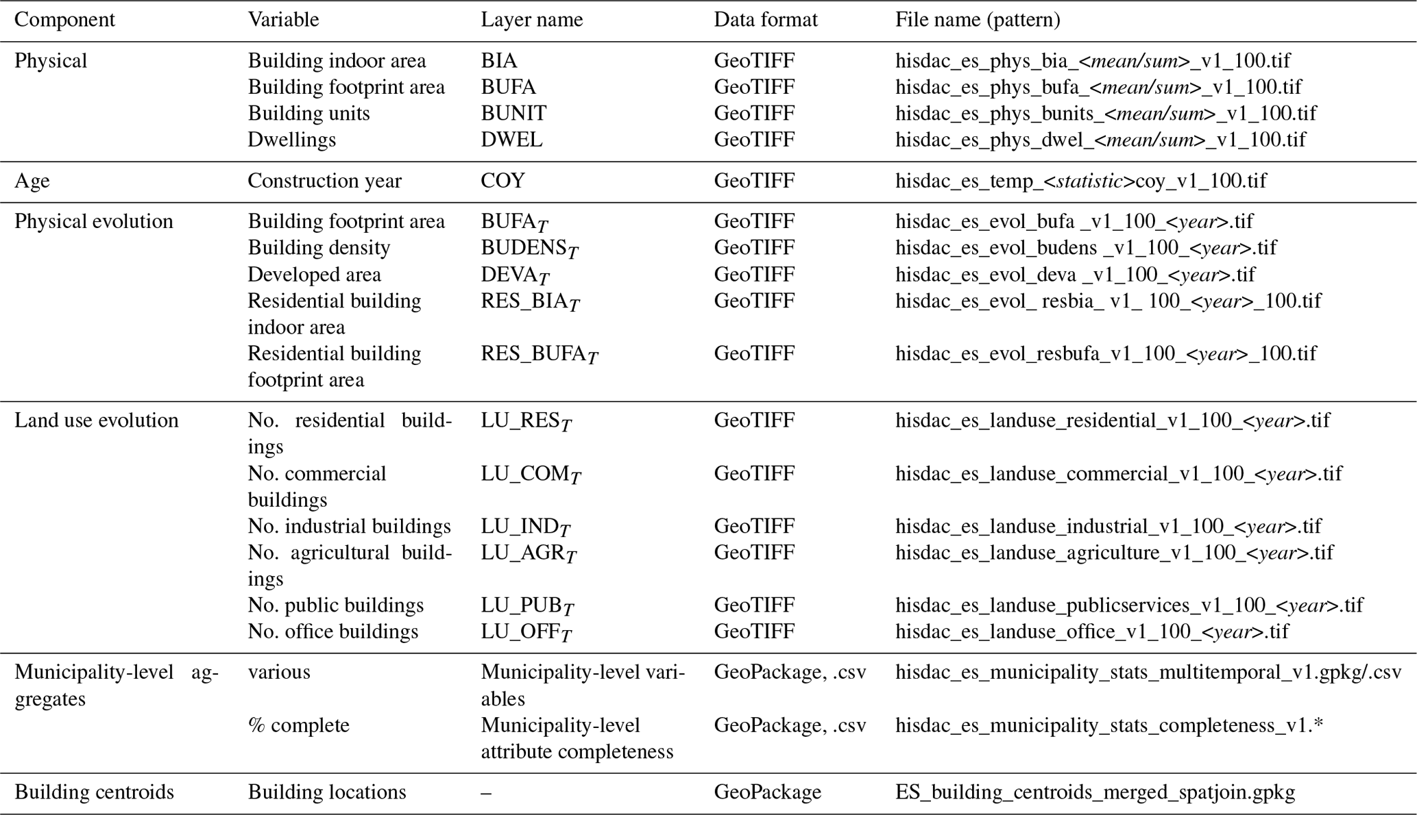
Cadastral building footprint data for Spain are hosted by national, regional, or provincial authorities. The data processing workflow consisted of the following steps: (1) we acquired around 12 000 000 building footprints and attributes as polygonal, geospatial vector data in Geographic Markup Language (GML) format from official web resources using automated and manual downloads (Sect. 2.1.1). (2) We harmonized the data (Sect. 2.1.2). (3) We aggregated the data into gridded surfaces and computed zonal statistics at the municipality level (Sect. 2.1.3). Furthermore, we evaluated the resulting gridded surfaces through comprehensive comparisons with a wide variety of independent spatial datasets (Sects. 2.2 and 4).
2.1 INSPIRE building data processing
2.1.1 Data collection
For most parts of Spain, cadastral building data are available through an ATOM interface. The ATOM feed format is an XML-based language that allows automated, web-based content retrieval by providing a machine-readable web interface (IBM, 2023). The ATOM XML files are organized in a hierarchical manner (see Table 1 for examples) and allow the building data to be accessed in GML format, at the municipality level. We created a Python script to automatically download these GML files (https://github.com/johannesuhl/hisdac-es, last access: 10 October 2023). In some cases (e.g., Basque Country, Navarre region, which have their own cadastral systems) we manually downloaded the data available as a Web Feature Service (WFS) (Table 1). All downloaded data were projected in UTM zone 30N (EPSG:25830).
Table 1Source data overview.
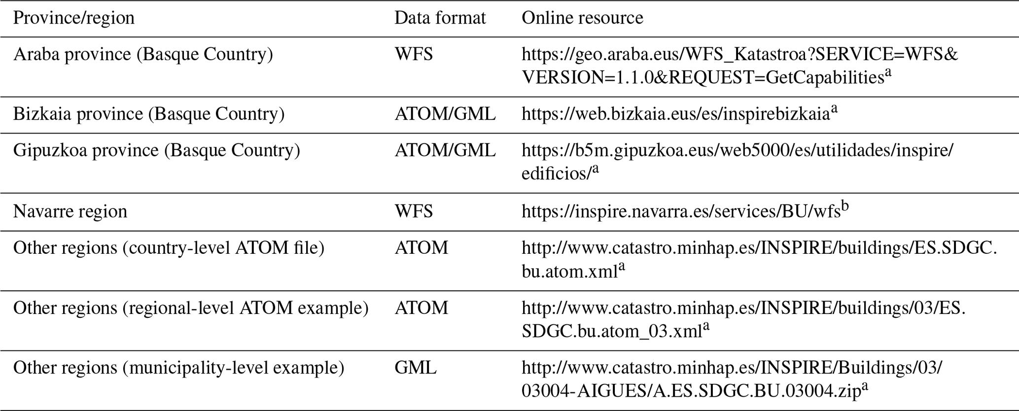
a Last access: 10 October 2023. b Last access: 15 October 2021. In the meantime, the WFS has been replaced by a repository available at https://filescartografia.navarra.es/2_CARTOGRAFIA_TEMATICA/2_7_CATASTRO/2_7_1_SHAPEFILE/ (last access: 10 October 2023).
2.1.2 Data preprocessing
After downloading and gathering the building data for over 8100 municipalities, covering all regions of Spain, we first calculated and attached the building footprint area (obtained after reprojecting to EPSG:3035) and converted the polygonal building footprint data to centroids, retaining all relevant attributes, to reduce the computational effort for the subsequent data processing. Despite the common INSPIRE framework, attribute names and building function classes differed slightly between the different data sources. Thus, we harmonized the data by renaming columns, and by applying a common building function classification scheme, including the six building function classes “residential”, “commercial”, “industrial”, “agricultural”, “public services”, and “office”. “Public services” is probably the broadest of these categories, including governmental buildings, but also health-related buildings and cultural institutions (e.g., churches or museums). Specifically, building function ontologies differed slightly for the data from the region of Navarre and the province of Araba and were consistent across the other regions/provinces. For example, commercial buildings in Navarre are labeled “trade” instead of “commercial”. The applied mapping scheme can be accessed on the HISDAC-ES GitHub repository (https://github.com/johannesuhl/hisdac-es/blob/main/landuse_mapping.csv, last access: 10 October 2023).
The gridded surfaces of HISDAC-ES are provided in three different spatial reference systems: (a) ETRS89 UTM zone 30N (EPSG:25830) for the Spanish mainland, Balearic Islands, and the exclaves Ceuta and Melilla located in northern Africa; (b) REGCAN-95 (EPSG:4083) for the Canary Islands; and (c) the reference grid of the European Environmental Agency (EEA), which is based on the ETRS89 Lambert azimuthal equal area projection (LAEA; EPSG:3035) and is commonly used for pan-European statistical mapping (e.g., CORINE Land Cover data), for all Spanish territory. This way, users can refer to the data in UTM/REGCAN for mapping purposes (north-oriented, angle-preserving), while the datasets in area-preserving LAEA projection can be used for statistical modeling and integration with other datasets (e.g., gridded statistical data from Eurostat (https://ec.europa.eu/eurostat/web/gisco/geodata/reference-data/grids, last access: 10 October 2023) or gridded Spanish census data (INE grid (https://www.ine.es/censos2011_datos/cen11_datos_resultados_rejillas.htm, last access: 10 October 2023)). Thus, we reprojected the building centroids into these reference systems, yielding two sets of harmonized building centroid data: (a) in UTM/REGCAN and (b) in LAEA projection.
After an initial examination of the attribute coverage and completeness, we decided to focus on six well-covered attributes, measuring different aspects of the built environment, including the construction year, building function, number of dwellings, number of building units, building indoor area, and building footprint area (Fig. 1). For clarity, the number of dwellings describes the number of housing units in residential buildings, whereas the number of building units also includes the number of units within non-residential buildings (e.g., number of commercial businesses within a building complex). Furthermore, the building indoor area represents the attribute “official area” and measures the gross indoor area (across all stories) within a building.
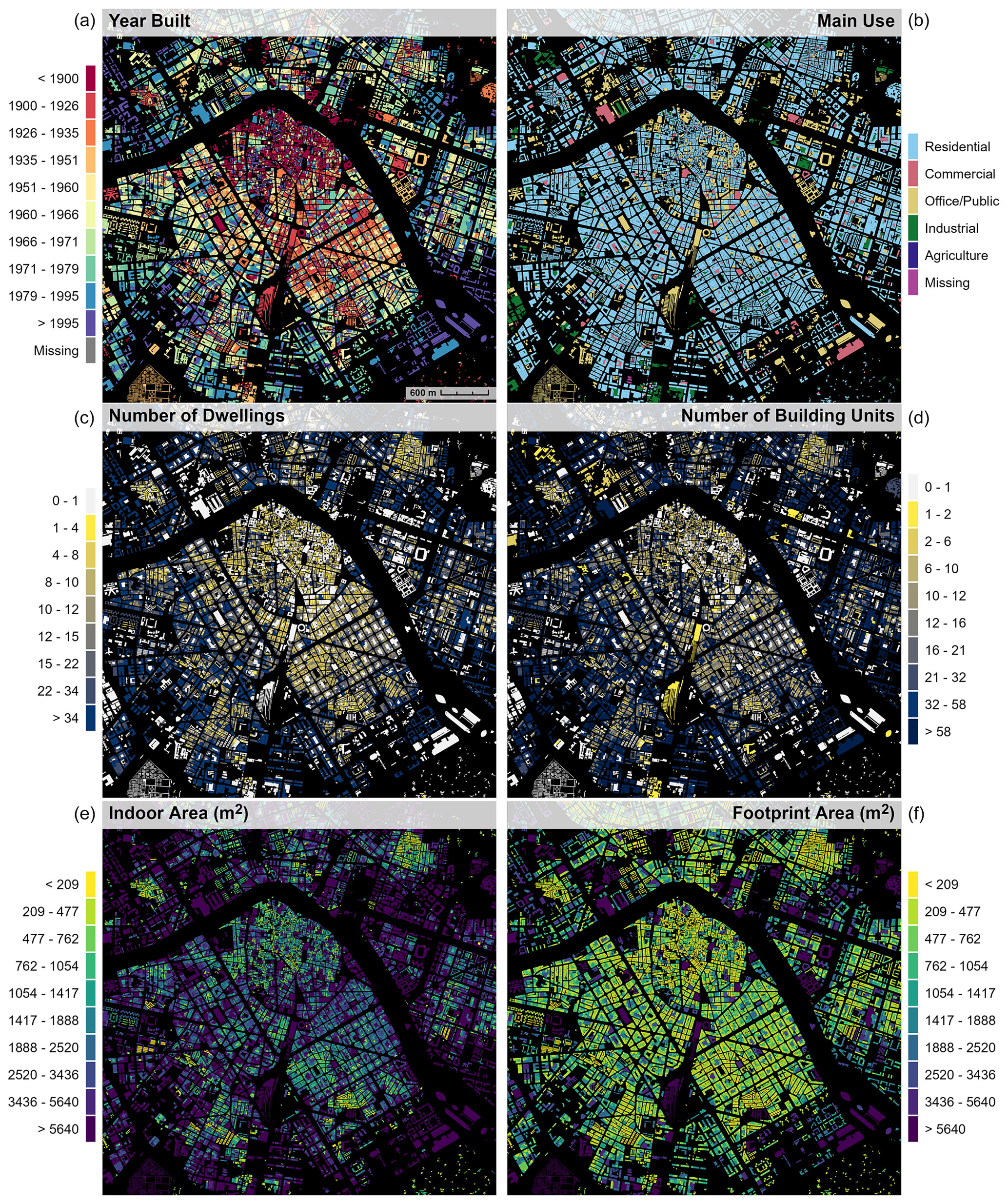
Figure 1Input data: INSPIRE-conforming building footprint data provided by the Spanish authorities, including several attributes. (a) Year built, (b) building use, (c) number of dwellings, (d) number of building units, (e) building indoor area, and (f) building footprint area. Data shown for the city of Valencia.
2.1.3 Data aggregation
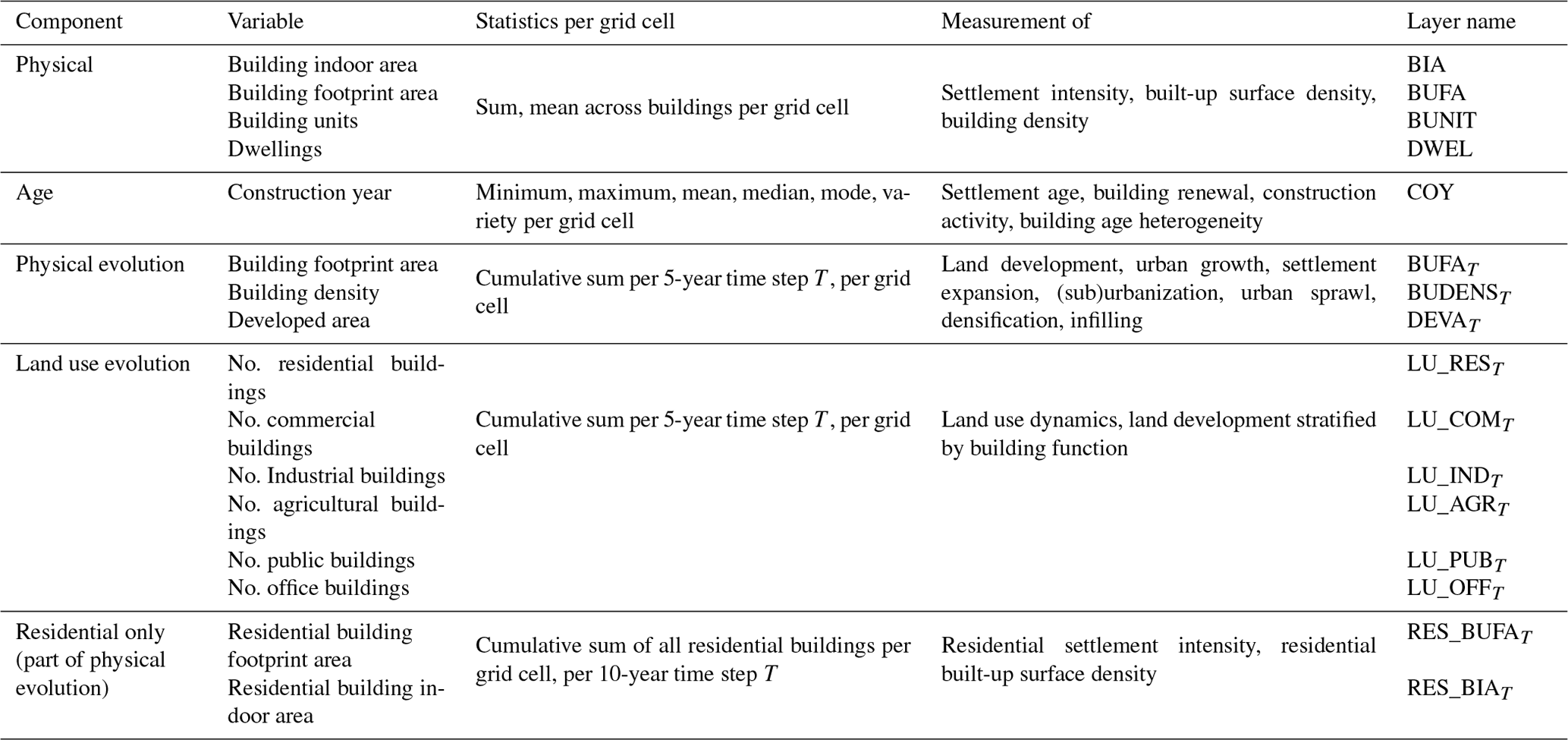
Based on the preprocessed, harmonized building data and the six selected thematic attributes, we created a range of different aggregated representations of the data. These aggregations include (a) spatial aggregation into grid cells within regular spatial grids of 100 m × 100 m, (b) aggregation to the municipality level by calculating zonal statistics per municipality polygon, and (c) temporal aggregation by stratification into different temporal classes. The combination of spatial aggregation and temporal stratification applied to the different thematic attributes yields a range of different sets of gridded surfaces. For example, we calculated the sum and the mean of the building units (BUNITS) and dwellings (DWEL) over all buildings within a given grid cell, as well as both the sum and mean building indoor area (BIA) and building footprint area (BUFA), based on the building centroids located within a grid cell. The resulting gridded surfaces represent physical features of the built environment. Similarly, we calculated the minimum, maximum, mean, median, mode, and the variety of construction years (COY) per grid cell, which measures settlement age (heterogeneity) and quantifies construction/remodeling activity within each grid cell. Thus, COY statistics describe the age-related features of the built environment.
We stratified the building records by their construction year into temporal classes (epochs) based on 5-year intervals (e.g., built-up before 1900, before 1905) and calculated the number (or density) of buildings (BUDENS) and the total building footprint area (BUFA) per grid cell in each of these epochs from 1900 to 2020. We further binarized these grid cells to measure developed area (DEVA) (i.e., grid cells containing at least one building) and undeveloped areas in each epoch. These gridded surfaces measure the physical evolution of the built environment in Spain. Similarly, we thematically disaggregated the building count surfaces per epoch based on the building function attribute of the buildings in each grid cell and epoch, yielding time series of function-specific building density layers, for six types of building functions (i.e., residential, commercial, industrial, agricultural, public services, and offices) as a proxy measure for built-up land use evolution from 1900 to 2020. Table 2 provides an overview of the gridded surfaces and spatial variables generated by these data processing steps. These surfaces quantify, for example, the building density (i.e., number of buildings per grid cell, BUDENS), the built-up surface density (i.e., building footprint area per grid cell, BUFA), or the built-up intensity (i.e., the total building indoor floor area per grid cell, BIA).
Table 2Overview of the gridded surfaces of the HISDAC-ES, measuring different components of the built environment, including the underlying variables and statistics.
As mentioned before, all gridded surfaces are available in UTM Zone 30N for the Iberian Peninsula, in REGCAN-95 for the Canaries, and in Lambert azimuthal equal area (LAEA) projection for the whole extent. For selected variables, we also provide a time series of zonal statistics, aggregated to the municipality boundaries2 (see Sect. 3.5). We created these zonal statistics based on (a) spatially joining the municipality identifier and area to each building centroid of our harmonized building dataset (point-in-polygon query) and (b) deriving statistics (sums, densities) for each municipality. All data processing, as well as the evaluation experiments and data visualizations, was implemented in Python 3.8, using libraries such as NumPy, SciPy, GDAL, GeoPandas, pandas, Matplotlib, PIL, and Esri ArcPy. The core component of our grid cell aggregation procedure is the “binned statistic 2D” function in SciPy (https://docs.scipy.org/doc/scipy/reference/generated/scipy.stats.binned_statistic_2d.html, last access: 10 October 2023). The overall processing workflow from the building data to the spatial layers of the HISDAC-ES is shown in Fig. 2.
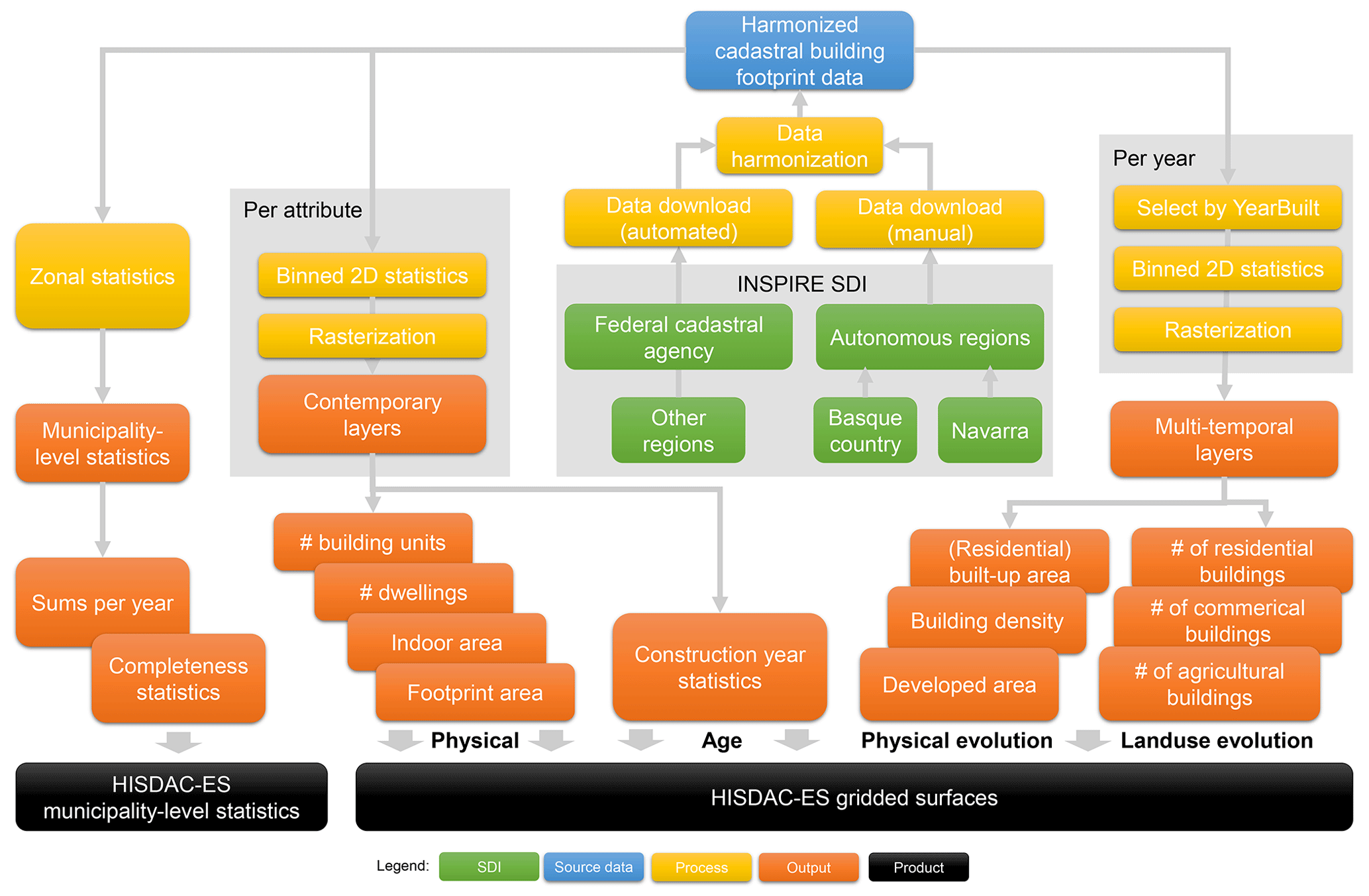
Figure 2Data processing workflow to create the spatial data layers of the HISDAC-ES, measuring multiple dimensions of the built environment in Spain from 1900 to 2020, obtained from cadastral building footprint data available via the INSPIRE Spatial Data Infrastructure (SDI).
2.2 Evaluation data and agreement assessments
As historical spatial data are generally scarce, the evaluation of the produced historical data is difficult. In order to evaluate the quality of the produced spatial layers in the HISDAC-ES as thoroughly as possible, we employed a range of independent datasets that exhibit coherence to the spatio-temporal processes measured by HISDAC-ES and carried out different evaluations and cross-comparisons. Specifically, we used three types of spatial data for these experiments: (a) recent, remote-sensing-derived datasets (i.e., the Global Human Settlement Layer (GHSL), CORINE Land Cover); (b) spatial–historical land use models (i.e., History Database of the Global Environment); and (c) historical cartographic data (i.e., historical maps and urban atlases) and orthoimagery. For most of these experiments, we implemented the following strategy: (1) when comparing HISDAC-ES to other gridded datasets, we downsampled the dataset of higher resolution to the dataset of lower resolution. This way, additional uncertainty introduced by resampling is kept to a minimum. (2) We conducted agreement experiments at the grid cell level, i.e., based on cell-by-cell map comparison or correlation analysis. (3) From these cell-by-cell-level comparisons, calculated agreement metrics within local or regional strata, defined by administrative boundaries or other classifications, are granular enough that we could assess regional variations of agreement, and large enough to ensure statistical robustness within each local stratum.
2.2.1 Global Human Settlement Layer (GHSL)
To evaluate the plausibility and reliability of the developed area (DEVA) layers from 1975 to 2015, we used built-up areas from the Global Human Settlement Layer (GHS-BUILT R2018, Florczyk et al., 2019) for comparison. The GHS-BUILT surfaces are derived from multispectral remote sensing data (Landsat sensors, Sentinel-2) and map built-up areas globally from 1975 to 2014, at a spatial resolution of 30 m (Fig. 3a, b). They are accompanied by a rural–urban classification (settlement model GHS-SMOD; Fig. 3c, d). GHS-SMOD is available at a resolution of 1 km and classifies each location on Earth into one of seven classes of urbanness, ranging from sparse rural settlements to high-density urban centers (Florczyk et al., 2019). While more recent versions of GHS-BUILT are available at the time of writing, we decided to use GHS-BUILT R2018A due to its fine spatial resolution and because a lot of work has been done and published to quantify the accuracy of GHS-BUILT R2018A across the rural–urban continuum and over time (e.g., Liu et al., 2020; Uhl and Leyk, 2022b, c), whereas little information is available on the accuracy of newer, multi-temporal GHS-BUILT datasets. For example, it has been reported that GHS-BUILT R2018A yields an average Intersection over Union of around 0.35 in 1975, in rural areas, to around 0.65 in 2018, in urban areas, respectively, for selected study areas in the United States (Uhl and Leyk, 2022b), and correlation coefficients of built-up surface fraction >0.7, compared to reference data for selected cities in China (Liu et al., 2020).
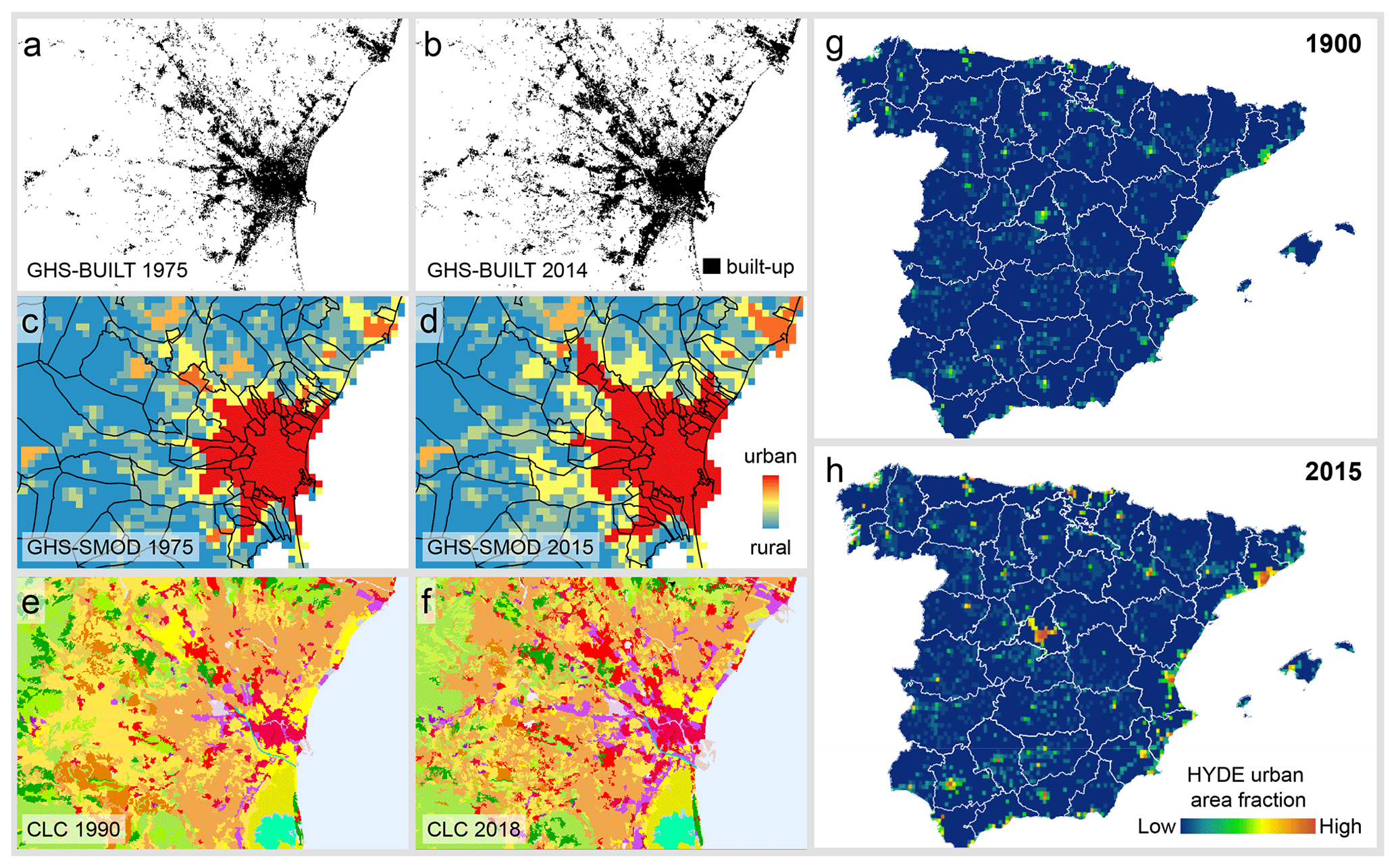
Figure 3Remote-sensing- and model-based evaluation data: built-up areas from GHS-BUILT R2018A in (a) 1975 and (b) 2014; GHS-SMOD rural–urban classes in (c) 1975 and (d) 2014; CORINE Land Cover data in (e) 1990 and (f) 2018; and urban area fraction from the HYDE v3.2 dataset in (g) 1900 and (h) 2015. Panels (a)–(f) show the city of Valencia, and panels (g) and (h) show mainland Spain and the Balearic Islands.
We resampled GHS-BUILT to the HISDAC-ES grid (i.e., upsampling from 30 to 100 m spatial resolution) for the epochs 1975, 1990, 2000, and 2015 and, thus, obtained binary grid cells (i.e., built-up vs. not built-up) for each epoch. To reduce spatial misalignment effects, we first upsampled the 30 m GHS-BUILT data to a 10 m × 10 m grid, nesting within the 100 m × 100 m HISDAC-ES grid, and then downsampled to the target grid, assigning 1 (built-up) if at least one 10 m grid cell within the target cell was labeled as built-up. We then quantified the agreement between the resampled, binary GHS-BUILT and the DEVA layers using Precision, Recall, and F1 score for each epoch and for each municipality. Specifically, we overlaid the binary raster surfaces of DEVA and GHSL and calculated the number of true positive (TP), false positive (FP), and false negative (FN) grid cells within each municipality polygon. These zonal statistics of binary agreement categories were then used to calculate municipality-level Precision, Recall, and F1 score. Moreover, we expected the agreement to vary across the rural–urban gradient (see Leyk et al., 2018; Uhl and Leyk, 2022a, b). Hence, we calculated these agreement metrics for each year, within each of the seven GHS-SMOD rural–urban classes, based on the zonal counts of TP, FP, and FN per SMOD class. Moreover, we generated a continuous rural–urban index for each municipality based on the GHS-SMOD layers, constructed from the weighted histogram of SMOD class instances within each municipality polygon (see Uhl et al., 2023c, for details), and assessed the municipality-level agreement trends across this rural–urban continuum (Sect. 4.1). Here, it is worth noting that we qualitatively compared the built-up areas from GHS-BUILT to the World Settlement Footprint (WSF) Evolution dataset (Marconcini et al., 2020a) and found high levels of agreement between these two datasets (Fig. A1). Thus, herein, we compared HISDAC-ES to GHS-BUILT only.
2.2.2 CORINE Land Cover data
While the comparison of DEVA and GHS-BUILT evaluated the presence/absence of buildings in the HISDAC-ES, we also used CORINE Land Cover data (CLC; Büttner, 2014) and compared them to the land use/building function layers in HISDAC-ES. For most years in which CLC data are available, their estimated accuracy exceeds 85 % (Büttner et al., 2021), while in the case of Spain, the accuracy of the CLC versions 2000 and 2006 has an estimated overall accuracy of >93 % (Diaz-Pacheco and Gutiérrez, 2014) in the Madrid region. Herein, we obtained CLC data, available at a spatial resolution of 100 m × 100 m for the earliest (1990) and most recent (2018) available epoch (Fig. 3e, f, also Fig. A1). As the grid underlying the HISDAC-ES LAEA version nests with the reference grid of the EEA, it also nests with the CLC grid. Thus, we overlaid the CLC surfaces with the land-use-specific building count layers of the respective years and cross-tabulated the building counts for each combination of INSPIRE building function class and CLC class on a cell-by-cell basis (Sect. 4.2).
2.2.3 History Database of the Global Environment (HYDE)
While the remotely sensed data from the GHSL and CLC allow for assessing the plausibility of the HISDAC-ES since 1975 and 1990, respectively, it does not provide any insight into the plausibility of the long-term trends (1900–2020) measured in the HISDAC-ES. To account for this, we employed the History Database of the Global Environment (HYDE V3.2; Klein Goldewijk et al., 2017), consisting of a set of global, gridded land use layers from 10 000 BC to 2015, which are model-based and available at a spatial resolution of 5′ × 5′ (approx. 6 km × 9 km in Spain). While the accuracy of built-up area estimates in the HYDE data is difficult to quantify due to a lack of historical reference data (Klein Goldewijk and Verburg, 2013), Uhl et al. (2021a) find relatively high agreement of urban growth trends extracted from HYDE and from the integrated processing of remote sensing data and historical maps. Specifically, we used the layer “urban area fraction” from HYDE for each decade from 1900 to 2015 (Fig. 3g, h) and aggregated both the building footprint area (BUFA) and developed area (DEVA) from the HISDAC-ES to the HYDE grid cells. We then conducted a correlation and regression analysis to quantify the agreement between BUFA, DEVA, and the total urban area as reported in HYDE, per grid cell. To account for potential regional differences in the agreement, we stratified our analyses into regions obtained from the NUTS-1 (Nomenclature of territorial units for statistics) administrative dataset (https://ec.europa.eu/eurostat/web/gisco/geodata/reference-data/administrative-units-statistical-units/nuts, last access: 10 October 2023) (Sect. 4.3).
2.2.4 Historical maps and orthoimagery
While the evaluation approaches described in the previous sections are based on measured or modeled data, they suffer from measurement error, resampling errors, and other incompatibilities that may bias the comparative analyses. Thus, we decided to include alternative, historical data sources in our evaluation analyses, allowing for a more unbiased evaluation of HISDAC-ES layers in early years. These data sources include (a) historical planimetric maps (shown for the city of Alicante in Fig. 4a), (b) aerial photographs from 1956 (Fig. 4b), and (c) an urban atlas (Remírez et al., 1998) depicting different urban development phases (Fig. 4c). While no quantitative information on the accuracy of these data sources is available, the underlying maps are handcrafted and based on manual interpretation of orthophotos, topographic measurements, or local domain knowledge and can be deemed to be relatively accurate. Specifically, we manually digitized the areas developed in different time periods for the city of Alicante and Madrid and obtained a similar vector dataset, depicting different historical urban development phases for the city of Valencia (courtesy of Carmen Zornoza-Gallego, 2022a). We quantitatively assessed the agreement between these historical urban extents and the MINCOY/DEVA layers (Sect. 4.4). Moreover, we visually compared the built-up areas depicted in planimetric topographic maps from around 19003 to the HISDAC-ES DEVA layer for several urban and rural places (Sect. 4.4). Finally, we manually delineated the approximate urban boundaries for the cities of Santiago de Compostela, Madrid, and Alicante based on aerial imagery from 19564 and compared them qualitatively to the developed areas in HISDAC-ES in the same year (Sect. 4.5).
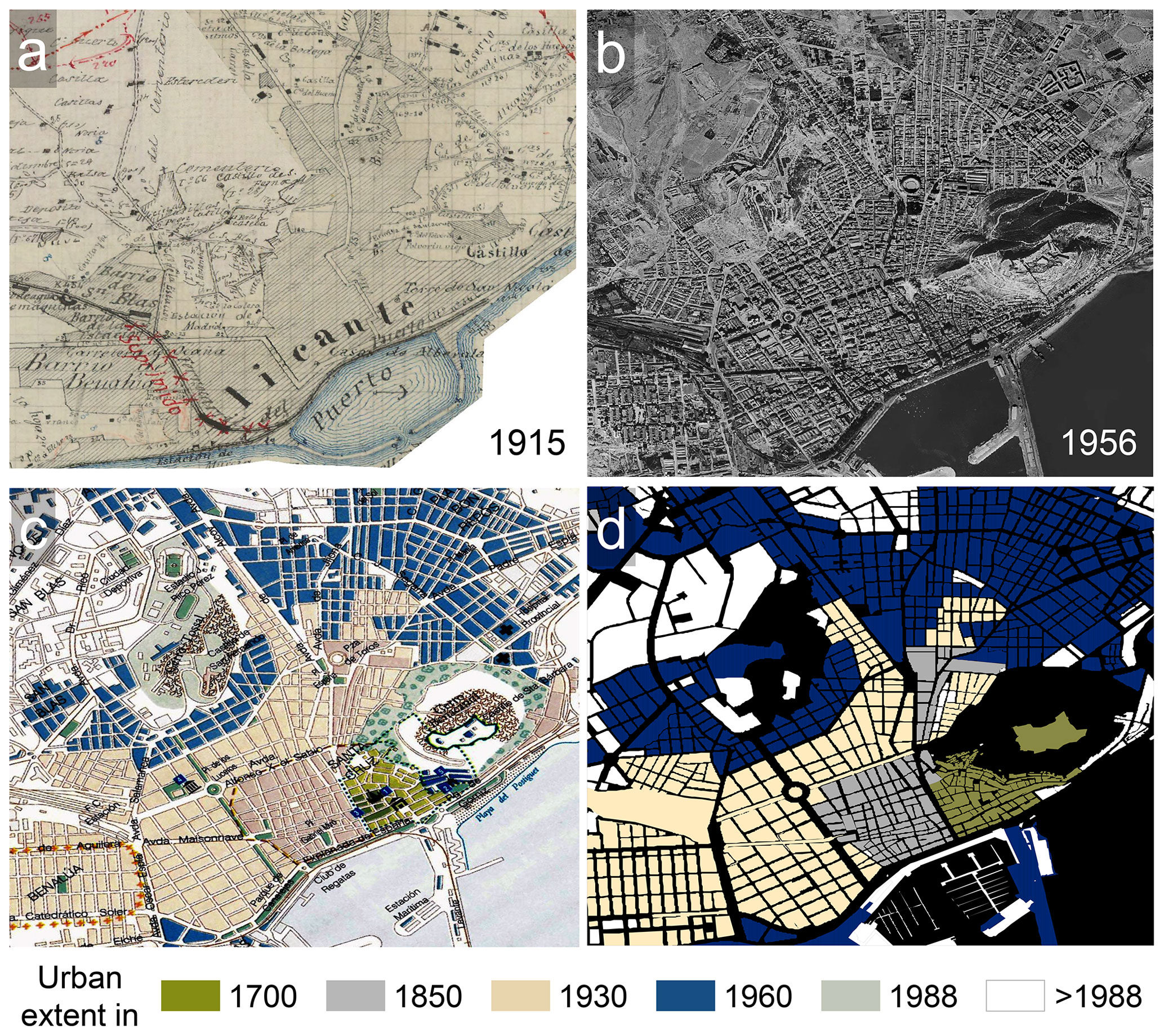
Figure 4Evaluation data based on historical cartography and orthoimagery: (a) Planimetría historical topographic map from 1910 (Minutas catastrones at scale 1:50 000; Instituto Nacional de Geografía, 2022), (b) historical aerial image from 1956 (Ortofotos AMS(B) 1956–1957), and (c) historical urban atlas illustrating different urban development phases (Remírez et al., 1988), and (d) urban areas for different time periods, manually digitized from (c). All datasets shown for the city of Alicante.
2.2.5 Attribute completeness
In addition to the comparison to external datasets, we also aimed to quantify internal uncertainties in the HISDAC-ES, or the underlying INSPIRE building data, respectively, by assessing the completeness and coverage of relevant building attributes at the municipality level (Sect. 4.6).
In this section, we present the different spatial layers contained in HISDAC-ES, resulting from the spatial aggregation and temporal stratification of the building data. This includes the gridded surfaces related to the four thematic components of HISDAC-ES (physical, age-related, physical, and land use evolution; Sect. 3.1 to 3.4) and the municipality-level statistics (Sect. 3.5).
3.1 Physical characteristics
Figure 5 displays the gridded surfaces measuring selected contemporary, physical features (in the year 2020) of the Spanish built environment, exemplarily shown for the city of Valencia. Surfaces showing the sums of these features exhibit interesting spatial patterns of the density of building indoor area (BIA) and footprint area (BUFA), decreasing from the city center towards the outskirts, whereas the density of dwellings (i.e., housing units) is higher in the outskirts than in the center part. The grid cell means of these variables are measures of (vertical/horizontal) building size and exhibit different patterns, illustrating the presence of large multi-apartment complexes in the outskirts and small, historical buildings in the center part of the city.
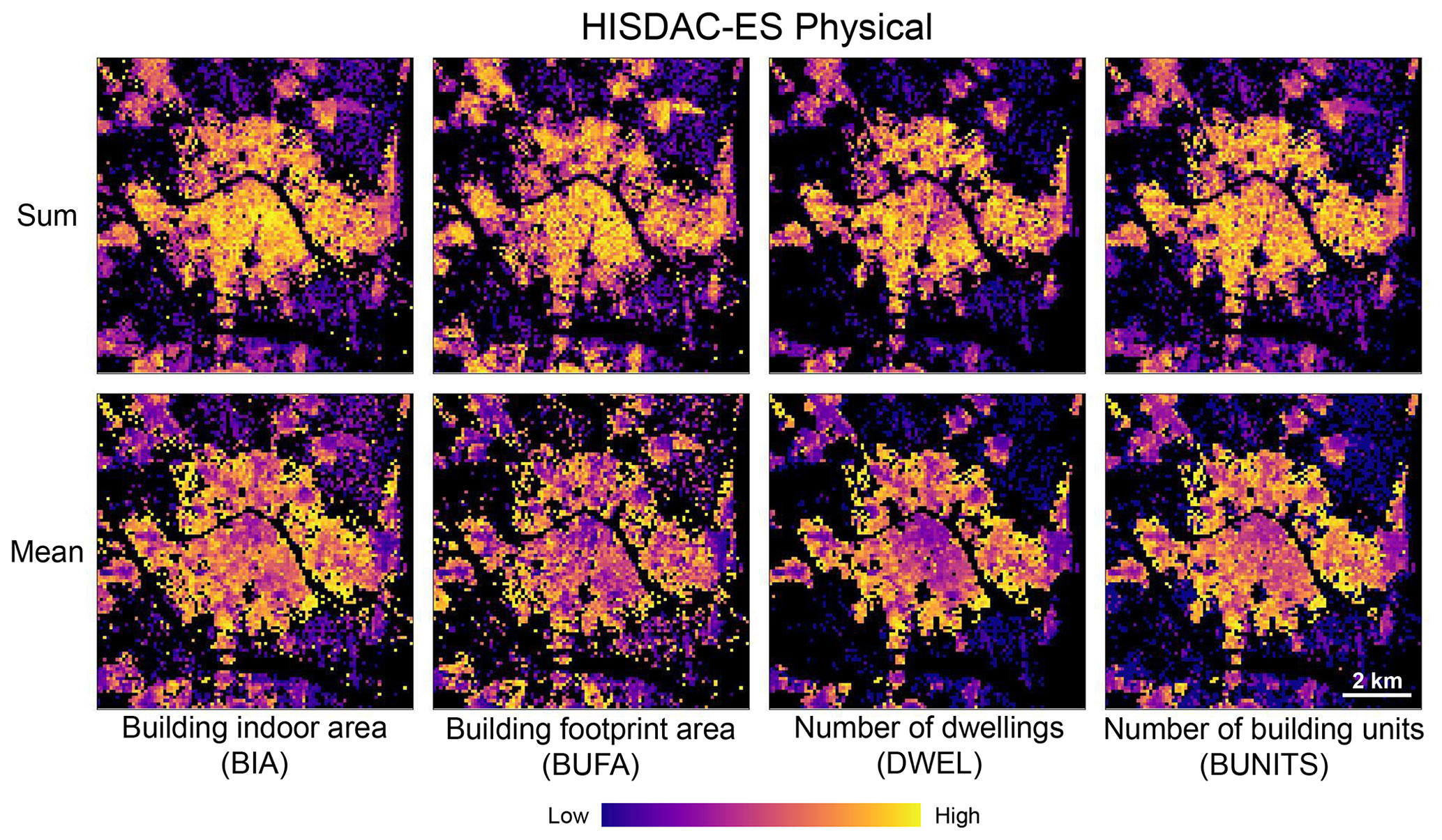
Figure 5Examples of the created gridded surfaces of the HISDAC-ES, quantifying physical characteristics of the built environment: building indoor area (BIA), building footprint area (BUFA), number of dwellings (DWEL), and number of building units (BUNITS). HISDAC-ES contains the sum (top row) and the mean (bottom row) of these variables per grid cell. All datasets shown for the city of Valencia.
3.2 Age-related characteristics
Age-related statistics of the Spanish building stock are measured by different statistics calculated using the construction year attribute of the buildings within each grid cell. For example, the minimum construction year (MINCOY) impressively shows the settlement age patterns in the metropolitan area of Valencia (Fig. 6), depicting the historical city core, as well as recently developed suburban areas in the urban fringe, and older settlements in the surrounding villages. Similar patterns can be observed in the mean (MEANCOY), median (MEDCOY), and the most frequent (i.e., mode) construction year (MODECOY). The maximum construction year (MAXCOY) per grid cell measures the year of the last modification of the building stock and, alongside the construction year variety (i.e., the number of unique construction years per grid cell, VARCOY), is a measure of construction activity, highlighting areas characterized by heavy urban renewal processes. Here it is worth noting that the construction year on record may also represent the year of the last building reformation, which introduces certain bias in the created surfaces (see Discussion section).
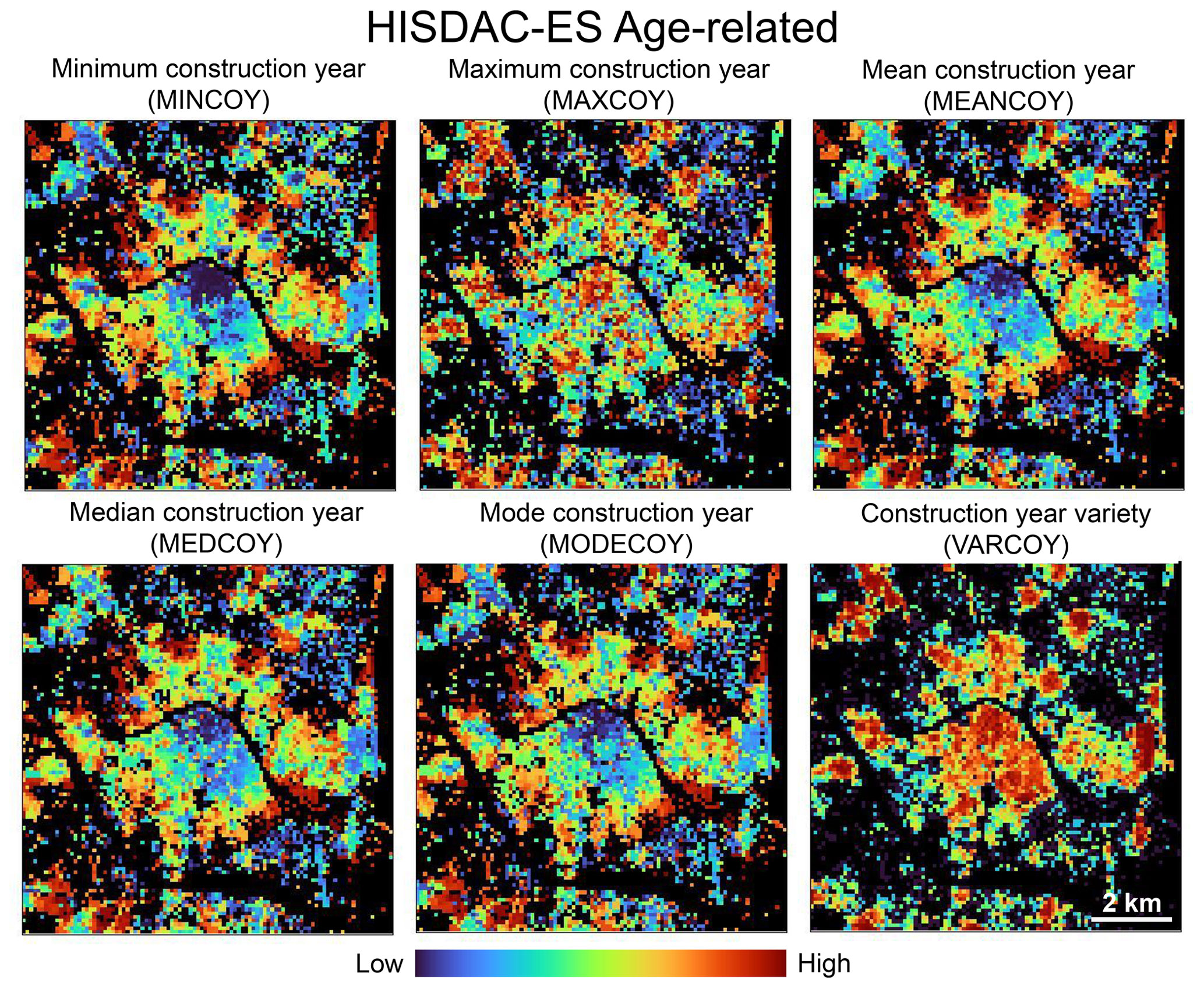
Figure 6Examples of the created gridded surfaces of the HISDAC-ES, describing building-age-related characteristics of the built environment: minimum construction year, maximum construction year, mean construction year, median construction year, mode (i.e., most frequent) construction year, and the variety (i.e., number of unique construction years) per grid cell. All datasets shown for the city of Valencia.
3.3 Evolutionary characteristics
Grid-cell-level statistics (i.e., sums of BUFA, counts/densities of buildings, BUDENS) stratified by the construction year attribute yield a time series of gridded surfaces measuring the long-term evolution of cities, towns, and villages. For example, the BUFA and BUDENS surfaces show how the built-up intensity (as measured by built-up surface density and building density) has increased from 1900 to 2020 (Fig. 7). These gridded surfaces uniquely document the long-term urban growth processes, measured at fine spatial granularity and over long time periods. The derived DEVA surfaces show developed/undeveloped land for each point in time, facilitating quantitative, multi-temporal analysis of urban form, e.g., using landscape metrics (Uhl et al., 2021b). The high temporal resolution (i.e., 5 years) of these multi-temporal layers enables the measurement of the evolution of urban extents and building density at fine spatial and temporal detail, as illustrated in a complete time series for the city of Valencia (Appendix Fig. B1). The additional stratification of the BUDENS layers by building function disaggregates the building stock spatially, by age, and by function. As an example shown in Fig. 7 (right column), industrial land use has heavily increased in suburban areas, especially in the northern suburbs (between 1900 and 1960) and later in the southern suburbs (after 1960).
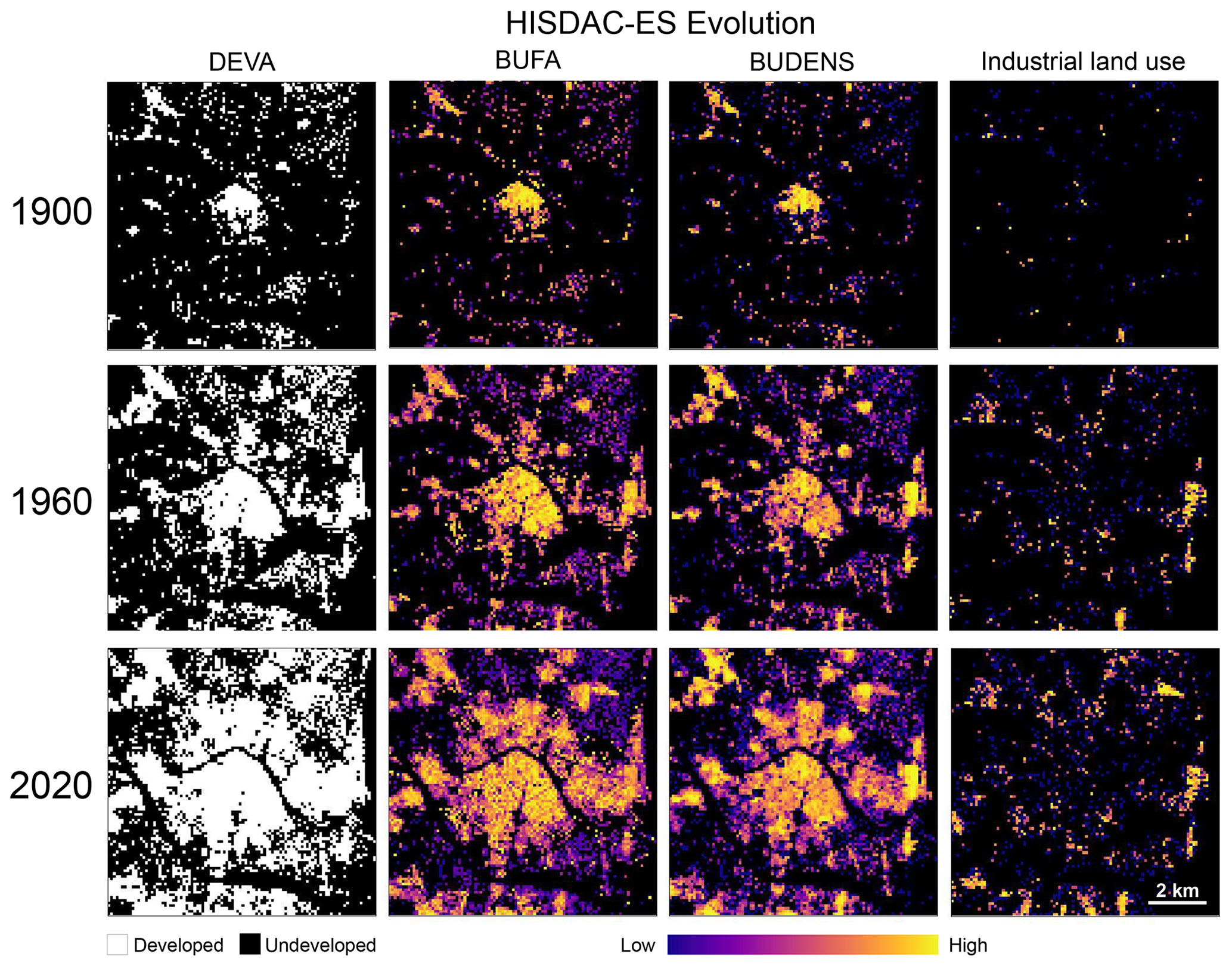
Figure 7Examples of the created gridded surfaces of the HISDAC-ES, quantifying evolutionary characteristics of the built environment: multi-temporal layers of developed area (DEVA), building footprint area (BUFA), and building density (BUDENS), as well as industrial land use in 1900, 1960, and 2020 (as one exemplary land use class). All datasets shown for the city of Valencia.
While the examples in Figs. 5–7 show the city of Valencia, we would like to emphasize the country-wide coverage of HISDAC-ES. For example, the minimum construction year surface (MINCOY) reveals commonalities and differences between settlement age patterns in different cities in Spain (Fig. 8), including polycentric development (e.g., Barcelona, Seville) and monocentric development (most other cities shown). Moreover, HISDAC-ES not only measures urban development across different cities, e.g., by means of the MINCOY surface (Fig. 8), but also long-term land development processes in rural areas, including towns, villages, and scattered, unincorporated settlements, as exemplified by the DEVA surfaces (Fig. 9). The DEVA layers reveal further detail on the spatial configuration of cities in early years, allowing, e.g., for the computation of historical, urban morphological indicators (Appendix Fig. B2). We also provide several supplementary animated data visualizations illustrating the value of HISDAC-ES for quantifying long-term urbanization processes (see Video supplement).
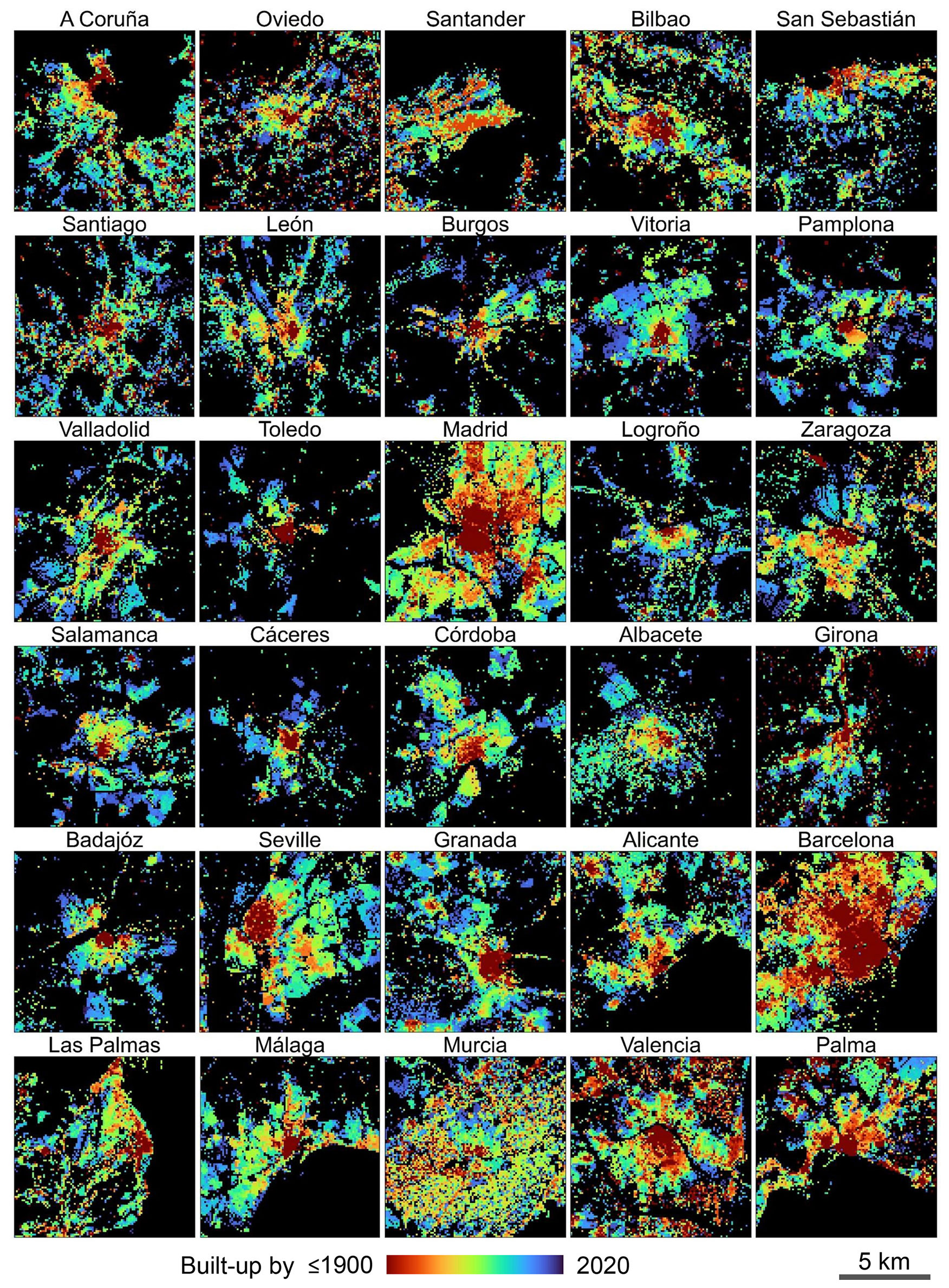
Figure 8HISDAC-ES settlement age surfaces for 30 cities in Spain: minimum construction year (MINCOY) shown for a selection of 30 cities, arranged in an approximate, quasi-geographic space (upper right shows the northeast; lower left shows the southwest).
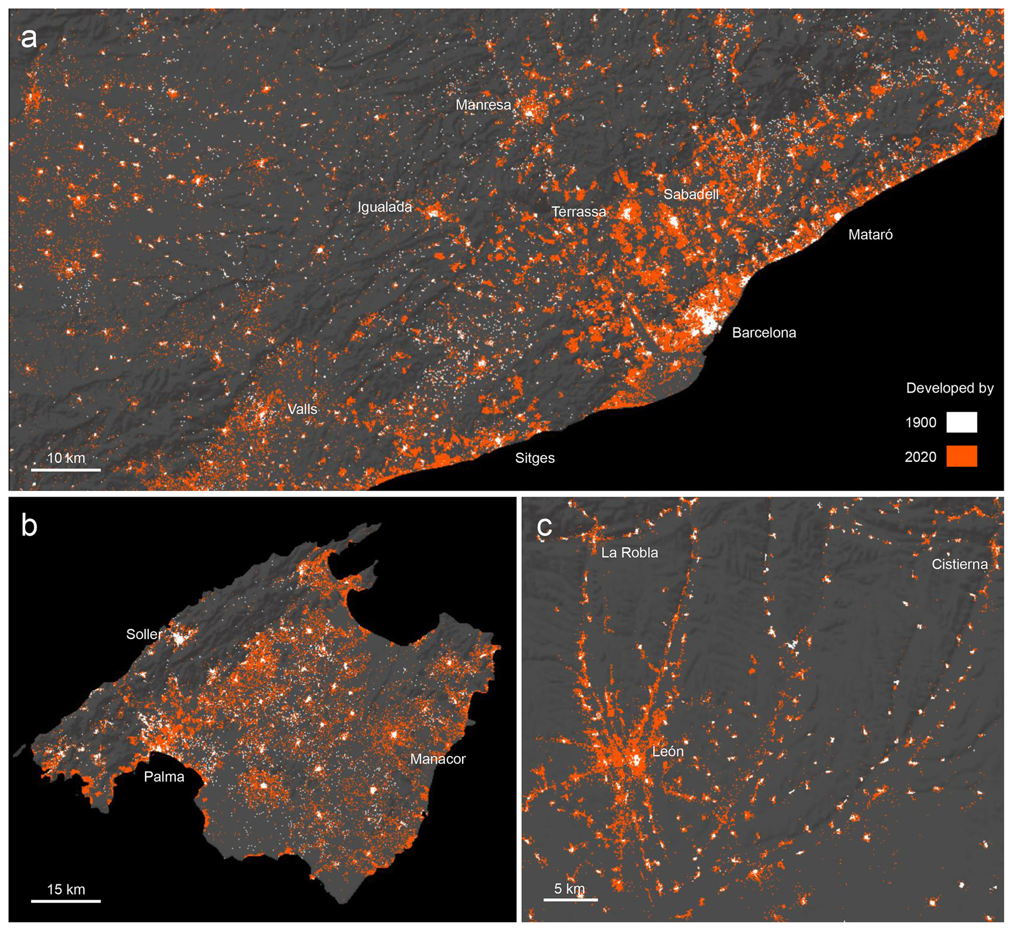
Figure 9HISDAC-ES multi-temporal surfaces of developed areas: DEVA layers for 1900 and 2020, shown (a) for Greater Barcelona, (b) for the island of Mallorca, and (c) for the greater León area. Basemap: Esri, USGS, NOAA.
3.4 Built-up land use surfaces
Lastly, we show the building density layers stratified by building function, measuring the spatial distribution of different built-up land use classes (Fig. 10). These gridded surfaces not only highlight the dominance of residential land use but also illustrate peri-urban clusters of industrial land use, as well as spatial patterns of commercial land use, which has a mixed clustered and scattered spatial pattern, or agricultural land use, mostly occurring in peri-urban areas to the northeast of Valencia. These surfaces, along with the corresponding multi-temporal land use surfaces (Fig. 7d) enable the quantitative assessment of land use specific evolution of the built environment and add a unique thematic component to the HISDAC-ES data layers. Besides the building density layers stratified per building function, we also provide the total building indoor area and building footprint area per grid, for residential buildings only (RES_BIA, RES_BUFA), facilitating the integration with historical population data and population disaggregation. We created RES_BIA and RES_BUFA for each decade from 1900 to 2020 (approximately in line with the decennial census), and in the LAEA grid only, as these layers are intended for statistical use.
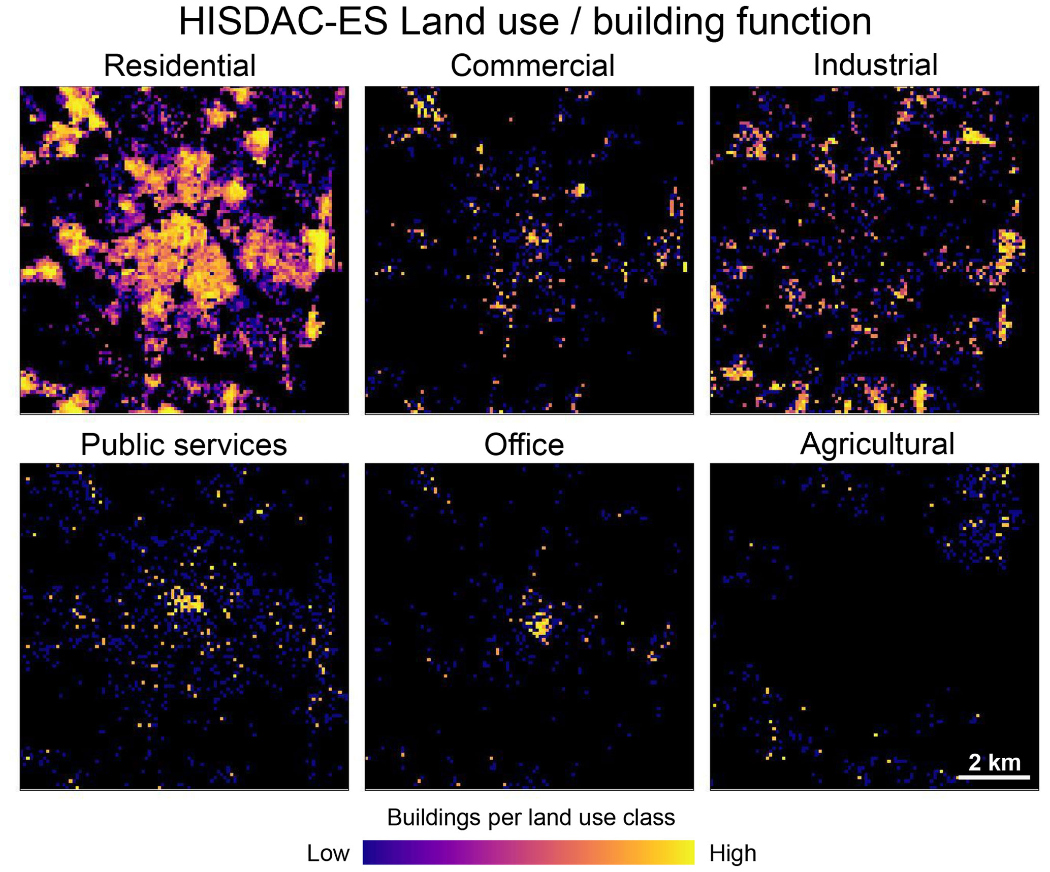
Figure 10Gridded surfaces describing the spatial distributions of different building function classes or building-related land use classes, shown for the city of Valencia in 2020.
3.5 Municipality-level statistics
We provide zonal statistics of building footprint data for over 8100 municipalities in Spain as tabular data and geospatial vector data. These datasets contain the zonal sums of selected variables (i.e., building counts, as well as BUFA, BIA, DWEL, BUNITS, RES_BUFA, RES_BIA) as well as corresponding densities (per municipality area) and allow for coarse-scale analyses, and for the joint analysis with historical population data, available at the municipality level. The visualizations in Fig. 11 illustrate the usefulness of such aggregated statistics to observe and quantitatively assess broad-scale settlement and building stock age patterns. These patterns can be interpreted in the context of historical settlement development but also provide insight into the contemporary building stock age and its spatial variation. As the absolute counts per municipality may be affected by regional trends of municipality area (Fig. 11, top row), we also provide these statistics as densities normalized by the municipality area, which show a different picture (Fig. 11, bottom row) (see Video supplement).
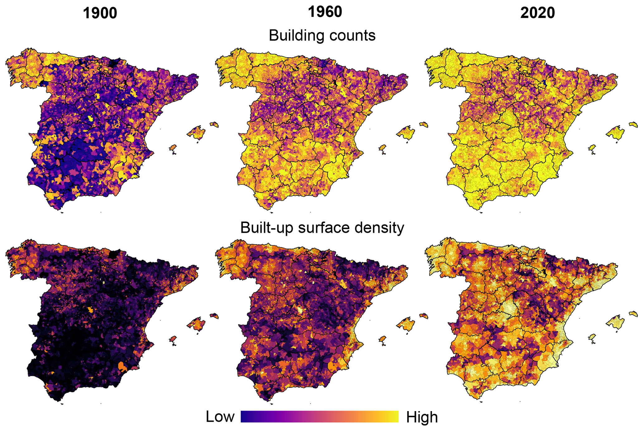
Figure 11Selected multi-temporal municipality-level statistics: building counts and built-up surface density per municipality in 1900, 1960, and 2020. See Appendix Fig. C1 for corresponding maps of the Canary Islands.
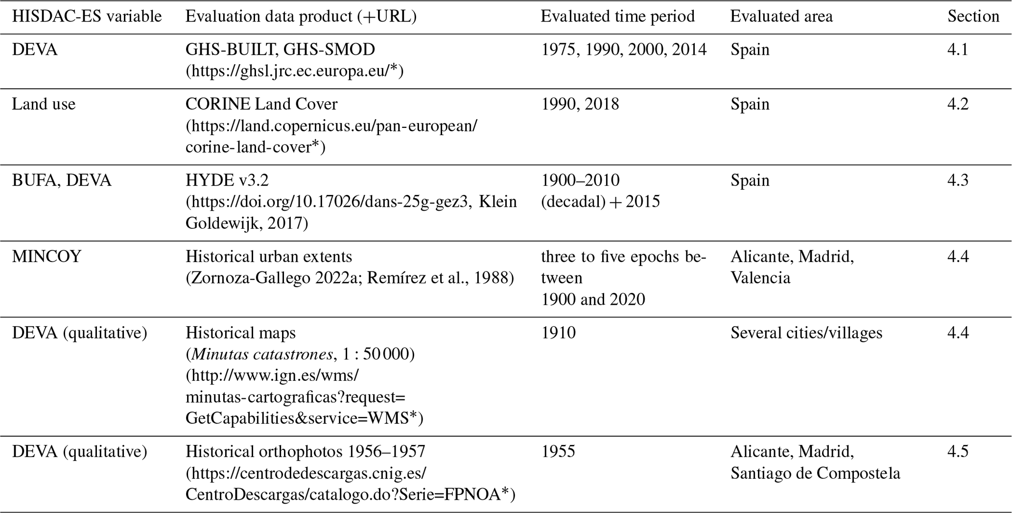
We compared the layers from HISDAC-ES to a variety of related but independent datasets to evaluate spatial, temporal, and thematic components of our data (Sect. 4.1–4.5). The various comparisons carried out are of either quantitative or qualitative nature and aim to evaluate the quality of the information contained in HISDAC-ES. The chosen evaluation datasets cover a range of data products of different sources (e.g., remote sensing, model-based hindcasting, historical cartographic sources) and different thematic domains (e.g., land use/land cover, built-up areas, urban areas) While none of the evaluation datasets are free from uncertainty, in particular for early points in time, we believe that demonstrating the coherence between the phenomena measured in HISDAC-ES and the respective evaluation datasets will shed light on the quality of HISDAC-ES from various perspectives. These evaluation efforts are summarized in Table 3. Moreover, we assessed the attribute completeness of the building data underlying HISDAC-ES (Sect. 4.6).
Table 3Overview of the comparative evaluation efforts for HISDAC-ES.
* Last access: 10 October 2023.
4.1 Multi-temporal built-up area evaluation (1975–2014)
The comparison of the developed area (DEVA) to built-up areas from GHS-BUILT reveals several trends: (1) the agreement between DEVA and GHS-BUILT changes from rural to urban areas. Specifically, the precision of DEVA is high in urban areas and low in rural areas (Fig. 12a). A low precision in an agreement assessment would indicate high commission errors, which in this case implies that DEVA labels much more grid cells as built-up than GHS-BUILT. This is encouraging as previous work has shown that GHS-BUILT tends to underreport built-up areas in rural regions (Leyk et al., 2018; Uhl and Leyk, 2022b), and thus, the DEVA layers appear to account for this shortcoming. Similarly, recall of DEVA is slightly lower in urban areas such as the Madrid region (Fig. 12a). As previous work revealed, GHS-BUILT tends to overestimate built-up areas in urban settings (i.e., roads are often classified as built-up). The DEVA layers are not affected by this type of misclassification, resulting in lower recall values. Hence, both low precision (rural settings) and low recall (urban settings) imply high accuracy in the DEVA layers, as the reference data (i.e., GHS-BUILT) suffer from the described shortcomings. (2) We observe an increase of precision over time (Fig. 12b), which is likely due to increasing completeness of built-up areas in GHS-BUILT, particularly in rural areas. Recall, however, shows a different trend over time (Fig. 12b), maximizing, on average, across all municipalities in 1990 and decreasing towards recent epochs. This is likely a combined effect of (a) increasing incompleteness in GHS-BUILT as we go back in time due to poorer quality of underlying Landsat data and (b) increasing incompleteness in DEVA as we go back in time due to a survivorship bias in the INSPIRE building footprint data. Specifically, new buildings that replace an existing (old) building will be attributed with the construction year of the replacement, and the building that existed prior to the replacement is not contained in our data. Thus, urban renewal causes this bias in our data, and this bias manifests in lower recall values towards early points in time.
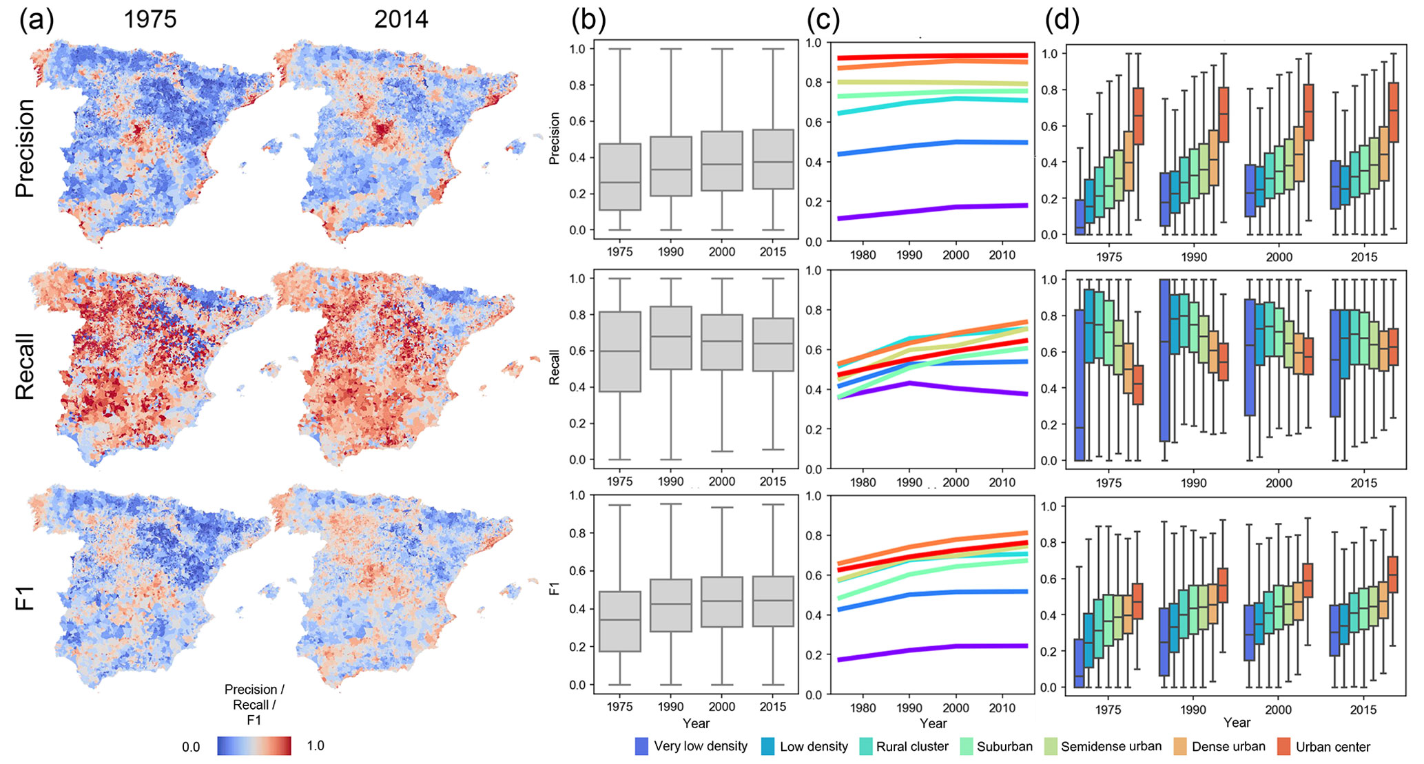
Figure 12Evaluation of the HISDAC-ES developed area (DEVA) in comparison to built-up areas from the Global Human Settlement Layer per municipality, over time, and across the rural–urban continuum, by means of map comparison. (a) Maps of municipality-level precision, recall, and F1 score in 1975 and 2014; (b) overall temporal trends of municipality-level precision, recall, and F1 score; (c) temporal trends of precision, recall, and F1 score calculated globally (i.e., at the country-level) within strata of the seven GHS-SMOD rural–urban classes; and (d) distributions of municipality-level agreement metrics within strata of a GHS-SMOD-based rural–urban index calculated per municipality. See Appendix Fig. D1 for corresponding maps of the Canary Islands. All agreement metrics are obtained by map comparison on a cell-by-cell basis at a spatial resolution of 100 m × 100 m, calculated locally within municipality boundaries in (a), (b), and (d) and calculated globally (i.e., overall metrics for the whole country) within areas delineated by GHS-SMOD classes in (c).
Looking at the agreement trends over time and across the GHS-SMOD rural–urban classes (Fig. 12c), we observe a sharp increase in agreement from rural to urban areas, and a slight increase over time, implying that the reliability of the DEVA layers is highest in urban centers. Lastly, the distributions of municipality-level agreement metrics across rural–urban strata confirm this trend (Fig. 12d). The peaks in recall in the low-density and rural cluster strata, across all years, indicate that the effects of incompleteness in the reference data (caused by omitting rural settlements) and in the DEVA (caused by survivorship bias) are of similar magnitude and, thus, cause higher levels of agreement. Here it is noteworthy that the more recent GHS-BUILT v2022 is likely to perform better in rural areas, and thus, precision of the HISDAC-ES is expected to increase in such areas, and the agreement gradients across the rural–urban continuum are expected to be less steep (Uhl and Leyk, 2023). However, as mentioned above, we prefer to use GHS-BUILT R2018A because its accuracy has been well studied and makes our interpretations more robust.
4.2 Land use evaluation 1990–2020
We cross-tabulated the land-use-specific building counts from HISDAC-ES in 1990 and 2020, within the land cover classes from CLC for the years 1990 and 2018 (Fig. 13). The absolute building counts per land cover class in Fig. 13a indicated that most buildings underlying the HISDAC-ES fall into urban fabric, industrial, or commercial areas; agriculturally used areas; and, to a lesser extent, areas characterized by forest (Fig. 13a). When plotting the proportions of buildings per HISDAC-ES land use class (Fig. 13b) or per CLC class (Fig. 13c), we observe more interesting patterns. For example, most buildings of any land use (except agriculture) are in areas of continuous urban fabric. Agriculturally used buildings are mostly located in areas classified as “complex cultivation patterns” in CLC. This indicates that the agricultural land use as reported in the INSPIRE building data is highly accurate. Moreover, in 2020, the proportion of buildings in “discontinuous urban fabric” has increased, as compared to 1990, which may be an effect of suburbanization and increasing low-density built-up areas. Finally, the cross-tabulation relative to the CLC classes shows that residential land use is the most dominant across all land cover classes, with a few interesting exceptions: industrial land use also has high proportions in CLC “industrial or commercial units”, and buildings attributed as “public services” in the cadastral data have a peak in “port areas” and “airport” CLC classes. Agricultural buildings peak in CLC classes “rice fields”, “annual crops”, and “agro-forestry areas”, which confirms the high levels of coherence between the two datasets. The peak of agricultural buildings in the “inland marshes” class may indicate higher levels of confusion between CLC classes “inland marshes” and “rice fields”, which may be difficult to differentiate. All these observations confirm that the land use information from the cadastral building data and the derived HISDAC-ES land use layers seems highly plausible. Note that there is a slight temporal gap between the two datasets, as the most recent CLC data are from 2018. However, we expect this discrepancy to be of minor importance.
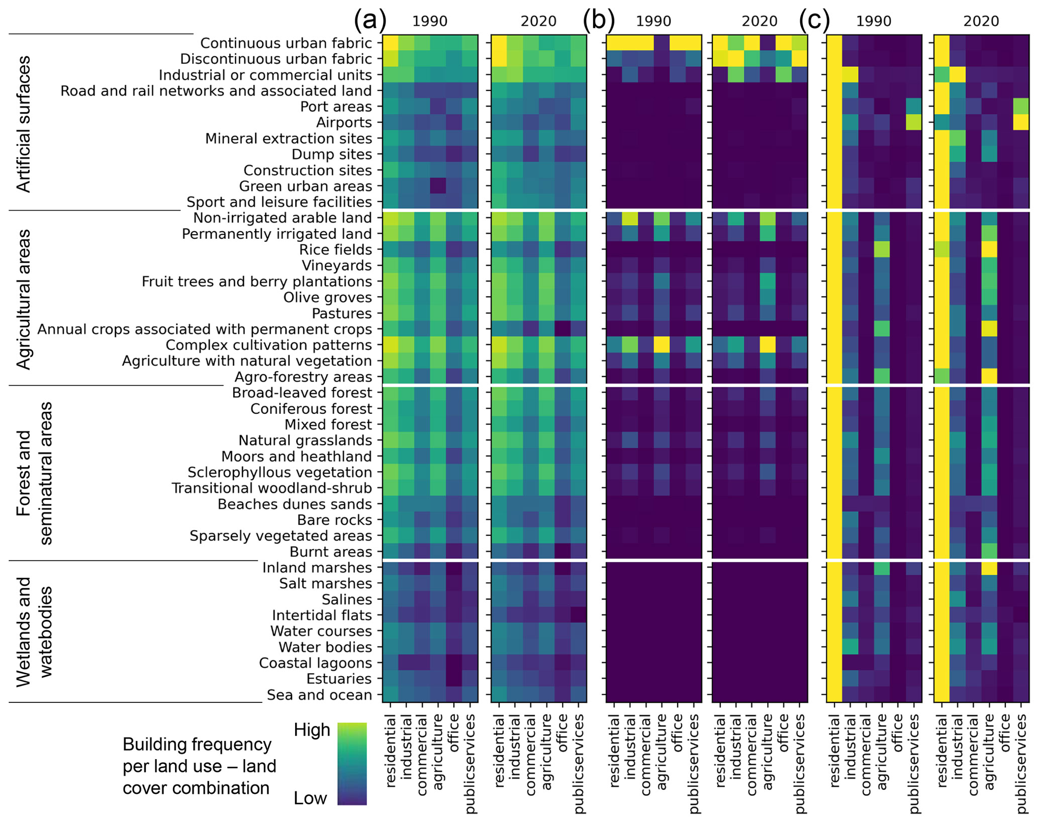
Figure 13Comparison of the HISDAC-ES land use data (columns) to land cover classes from CORINE Land Cover (rows) for the years 1990 and 2018. The heatmaps show the number of buildings (BUDENS) assigned to grid cells within each combination of HISDAC-ES land use and CLC classes. These bidimensional frequency maps are shown in three variants showing (a) absolute building counts, (b) proportions of buildings per HISDAC-ES land use class, and (c) proportion of buildings per CLC class. Note that the 2020 HISDAC-ES data were compared to the 2018 CLC data.
4.3 Long-term trajectory evaluation (1900–2015)
While the comparisons of HISDAC-ES to GHS-BUILT and CORINE Land Cover data focus on recent decades, the comparison to HYDE's urban fraction estimates examines the long-term agreement with the BUFA and DEVA evolution layers. We observe that the correlation between urban area fraction and BUFA is high after 1980 (i.e., >0.8 for most regions) and decreases as we go back in time but is still at around 0.6 in 1900, in most regions (Fig. 14a). This drop in correlation could be explained by the previously mentioned survivorship bias in HISDAC-ES but could also be attributed to uncertainties in the model-based urban area fractions in HYDE. The correlation to DEVA (Fig. 14b) shows a similar trend but slightly lower levels of correlations. Interestingly, correlations are highest in the southern region (i.e., Andalucia), possibly due to low levels of building stock renewal and, thus, a weaker effect of the survivorship bias in the HISDAC-ES data. Interestingly, correlations reach an early peak for the Madrid region (1960s for BUFA, 1930s for DEVA) and then drop. Such a decreasing agreement towards recent epochs could be related to heavy (peri-)urban renewal in the Madrid region, which would be less well captured in HISDAC-ES (cf. Sect. 4.5). Besides this comparison of quantitative measures per grid cell, we also compared the agreement between developed and undeveloped grid cells in DEVA and HYDE, as measured by the time series of F1 scores in Fig. 14c. We observe extremely high agreement (>0.95) in recent decades and just slightly lower F1 scores in the beginning of the 20th century. These high levels of agreement of the HISDAC-ES and model-based urban area estimations from HYDE underline the high quality of the HISDAC-ES evolutionary layers. It is noteworthy that the high F1 scores may be an effect of the relatively low spatial resolution of HYDE (5′ × 5′ grid cells).
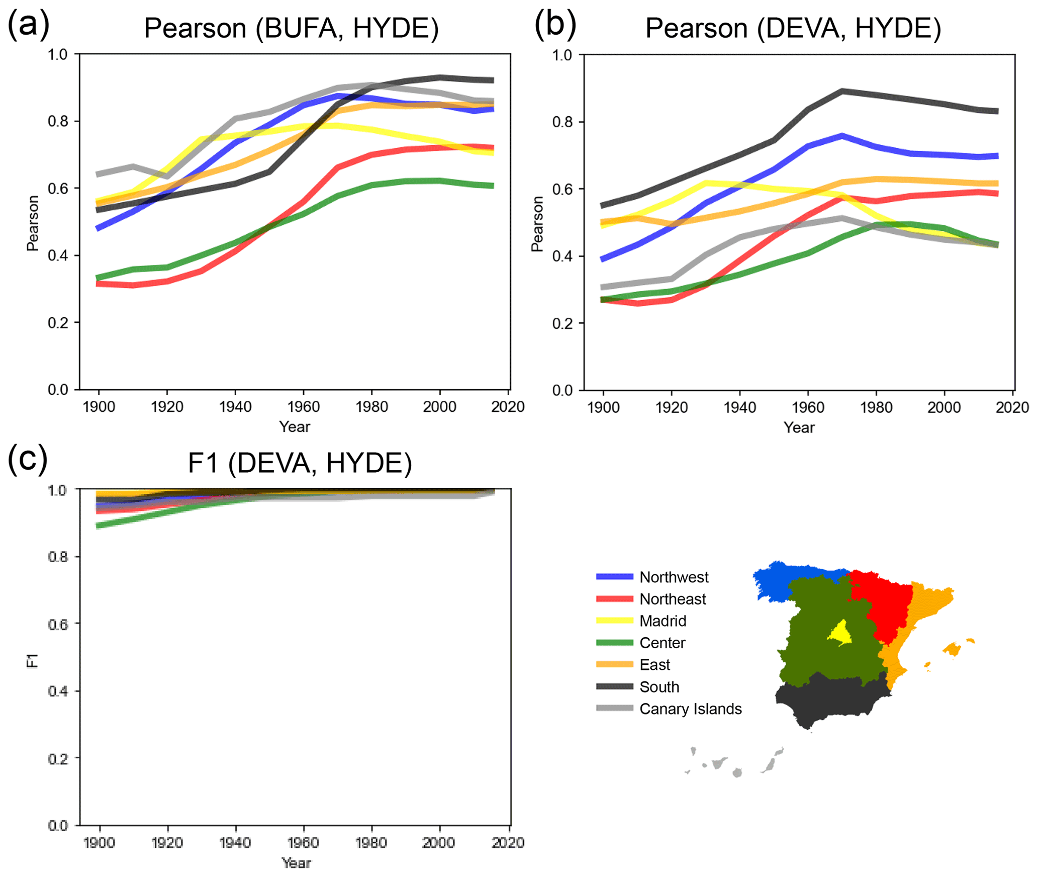
Figure 14Regionally stratified agreement analysis of HISDAC-ES developed area (DEVA) and building footprint area (BUFA) variables against HYDE urban area estimates. (a) Time series of Pearson's correlation coefficient of BUFA and HYDE, (b) time series of Pearson's correlation coefficient of DEVA and HYDE, and (c) time series of F1 scores based on developed vs. non-developed grid cells in the HISDAC-ES and HYDE urban area fraction (5′ × 5′ grid cells). Regional stratification was done based on the seven NUTS-1 regions (https://ec.europa.eu/eurostat/web/gisco/geodata/reference-data/administrative-units-statistical-units/nuts, last access: 10 October 2023).
4.4 Comparison to historical maps
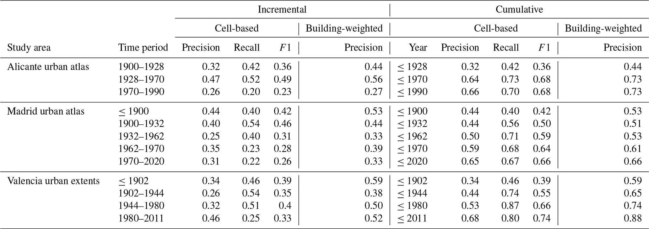
The previous evaluations are based on either remotely sensed data or model-based reference data. Thus, those datasets are limited in their temporal coverage or suffer from uncertainty themselves. Hence, we used multi-temporal urban areas manually digitized from historical maps, covering the period from approximately 1900 to present, for the cities of Alicante, Madrid, and Valencia (Fig. 15). These extents were manually digitized for Alicante and Madrid from an urban atlas (Remírez et al., 1988; Valencia data are courtesy of Carmen Zornoza-Gallego), resulting in increments of urban area newly added in a given time period (see Fig. 4a, b). We rasterized the resulting vector data in the HISDAC-ES grid, encoding the earlier year of each time period (Fig. 15a). For each city, we reclassified the MINCOY surface to match the settlement age categories from the digitized urban areas (Fig. 15b) and calculated agreement measures for each city, based on both the cumulative urban area per point in time and the newly added built-up area in each period (Table 4). As the MINCOY surface only encodes the year of earliest settlement per grid cell, disregarding the settlement density in that year, we also used the BUDENS layers for the respective years (shown for 1900 and 2015 in Fig. 15c, d), to weight each grid cell by its building density. We did this because we assumed that misclassifications are more likely in sparsely populated areas, likely not contained in the urban extents from the historical urban atlases due to generalization. Thus, agreement metrics based on building counts rather than grid cell counts would be more representative and realistic for a comparison between these two datasets. Based on this evaluation strategy, we observe the following:
-
Agreement levels are generally relatively low (F1 between 0.28 and 0.74). This may be attributed to the survivorship bias in HISDAC-ES but also due to definitional differences; i.e., HISDAC-ES measures built-up area, while the urban extents derived from historical atlases measure urban area and, thus, are already a generalized representation of the developed land at a given point in time. They are likely to omit low-density, scattered, peri-urban settlements but include roads, impervious surfaces, and intra-urban green spaces (e.g., parks and cemeteries), which are not directly measured in HISDAC-ES, which is based on the presence of built structures only.
-
Recall is higher than precision. Low precision indicates high commission error (i.e., overestimation), likely because peri-urban, rural settlements are contained in HISDAC-ES but not in the urban extents due to generalization and the (arbitrary) definition of the urban boundaries in the historical urban atlases, similar to what we observed in the comparison to the GHSL (Sect. 4.1).
-
Agreement for cumulative urban extents is higher than for incremental time slices. This effect is to be expected, as the confusion between historical increments is irrelevant when comparing the total built-up/urban area at each point in time. As the urban areas (and the increments) in early time periods can be small, misclassification is more likely, also due to higher levels of survivorship bias in HISDAC-ES for early time periods.
-
Precision based on the number of buildings is higher than precision based on the number of “occupied” grid cells. This indicated that grid cells label ed as “built-up” in HISDAC-ES but not in the historical urban areas tend to have low building density, confirming our aforementioned assumption that low-density settlements are not mapped in the historical urban extents.
-
For cumulative urban extents, precision and recall increase over time. This is a direct effect of the survivorship bias, manifesting in higher omission errors (and thus lower recall) as we go back in time. Moreover, the proportion of scattered low-density settlements (which are not contained in the historical urban atlases) in relation to dense, urban settlements was higher in early than in recent epochs, resulting in an increase of precision over time.
Moreover, the agreement levels are relatively similar across the three cities under study, implying that these observations are likely to be generalizable at least across the larger cities in Spain. Despite the low absolute numbers of the agreement metrics reported in Table 4, which are likely due to definitional differences, the observed trends are in line with theoretical expectations (e.g., survivorship bias decreases over time) and with evaluation results of the HISDAC-US (Uhl et al., 2021c), indicating similar characteristics of the historical settlement layers derived from cadastral/property data in the United States and in Spain. Confusion matrices underlying the agreement metrics shown in Table 4 can be found in the Appendix Fig. E1.
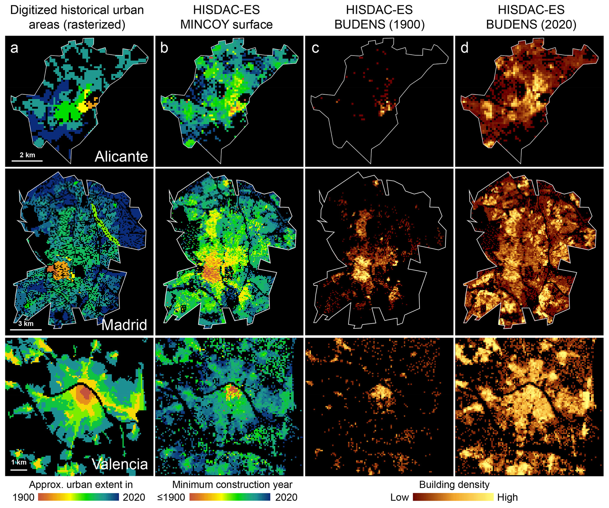
Figure 15Data used for the quantitative comparison of the HISDAC-ES to historical urban extents, derived from historical maps for the cities of Alicante (top row), Madrid (middle row), and Valencia (bottom row): (a) historical urban areas digitized from historical maps after rasterization, (b) the HISDAC-ES MINCOY layer, and the HISDAC-ES building density layers for (c) 1900 and (d) 2020. Data source of the historical urban extents for Valencia: courtesy of Carmen Zornoza-Gallego. Figure in the lower left corner adapted from Zornoza-Gallego (2022a).
Table 4Map comparison results of urban areas digitized from historical maps and HISDAC-ES settlement age surface (MINCOY), for both increments (i.e., newly developed grid cells between two points in time) and cumulatively (i.e., for the total developed land at a given point in time. Note that there is a slight temporal gap in the earliest Madrid epoch, where MINCOY from 1900 is compared to urban extents from 1892.
The qualitative comparison of the DEVA layers and planimetric historical maps (predecessors of the Minutas catastrones from 1870–1950, at scale 1:50 000) confirms the previously made observations. As shown in Fig. 16, the DEVA layer (for 1900) mimics the urban areas as depicted in the maps quite well, with some omission errors mainly in peri-urban areas, e.g., for Madrid, Seville, and Terrassa. This could indicate that building replacements (causing survivorship bias in the HISDAC-ES) tend to occur least in the medieval city centers, which are subject to monument protection (assuming concentric growth patterns). Moreover, these disagreement patterns may also be due to temporal inconsistencies between DEVA (1900) and the planimetric maps, which may have slightly different temporal references. In the small villages around Hornillos del Camino (Burgos) (Fig. 16 right column) we rather observe over- than underestimation. This could indicate that in rural, economically less prosperous areas, where less building remodeling occurs, the original building stock is still dominating, and, thus, the HISDAC-ES is less affected by survivorship bias. This observation may imply higher levels of data quality in small, rural places, a promising perspective for long-term settlement modeling in the often under-studied rural settings. The bottom row (Fig. 16c) shows the contemporary (i.e., 2020) building densities, illustrating a positive association between building density and settlement age.
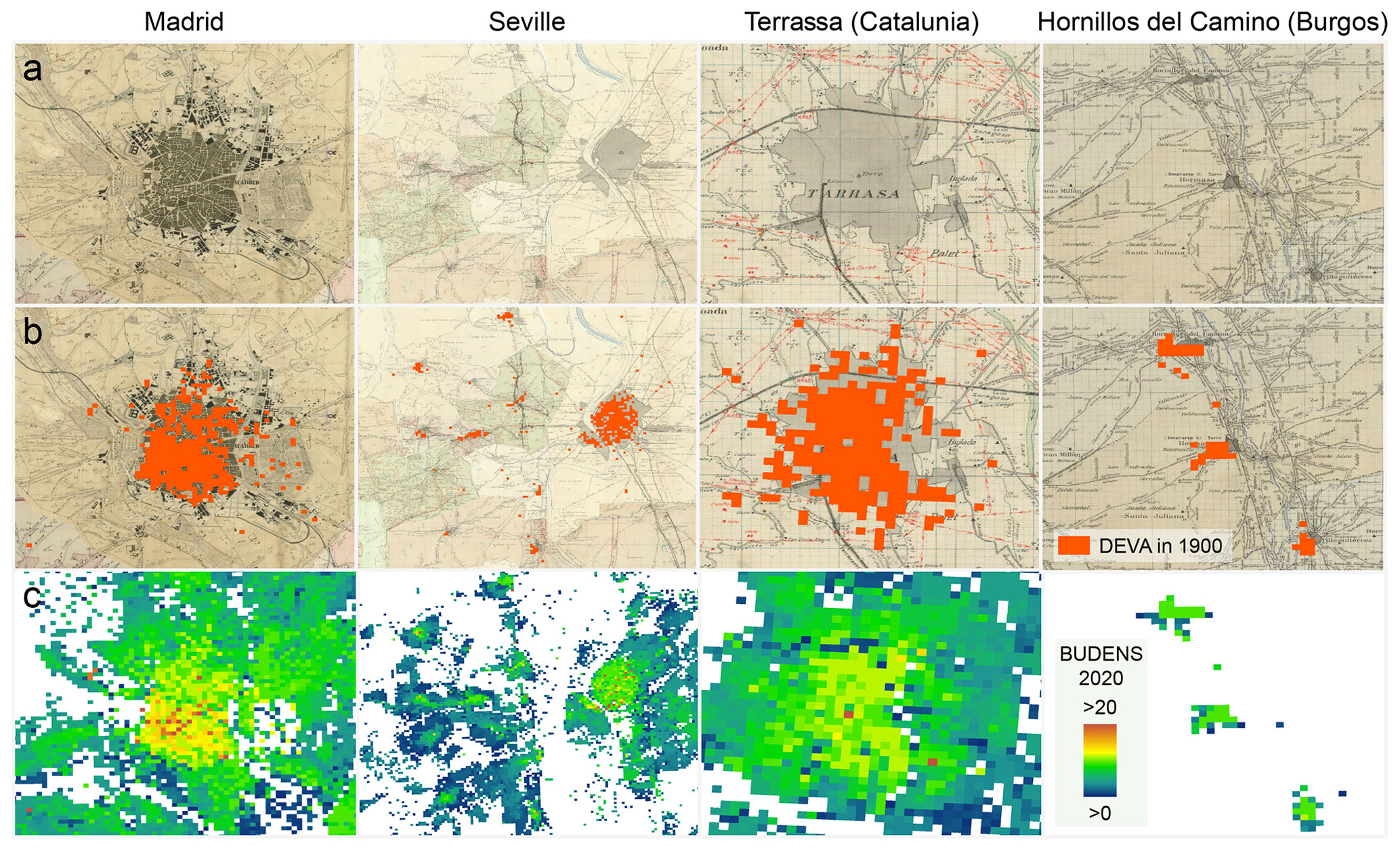
Figure 16Visual comparison of HISDAC-ES developed areas (i.e., DEVA layer in 1900) with historical maps. (a) “Planimetría” maps (b) overlaid with DEVA in 1900 and (c) contemporary building density layer (BUDENS) in 2020), illustrating the change between 1900 and 2020. Each layer is shown for Madrid, Seville, Terrassa (Catalonia), and Hornillos del Camino (Burgos). Historical map source: Instituto Nacional de Geografía (2022).
4.5 Comparison to historical orthophotos from 1956
The urban extents manually digitized from historical orthophotos acquired in 1956 show the urban boundary in those years in Alicante, Madrid, and Santiago de Compostela (Fig. 17a, b, c). When we overlay these boundaries to the built-up areas from HISDAC-ES in the same year, we observe varying levels of agreement: In Alicante the agreement is relatively high (Fig. 17d), as well as in Santiago (Fig. 17f), whereas we observe higher levels of disagreement in the Madrid data (Fig. 17e), mainly occurring in suburban areas. While some of the disagreement may be attributed to differences in definitions (i.e., the urban boundaries drawn in the orthophotos only include dense, urban settlements), in the Madrid case there are additional issues, related to notable activities of urban renewal in previously informal settlements (e.g., the Entrevías neighborhood; example 2 in Fig. 17e). See Fig. F1 for a more detailed discussion of historical reasons for these discrepancies.
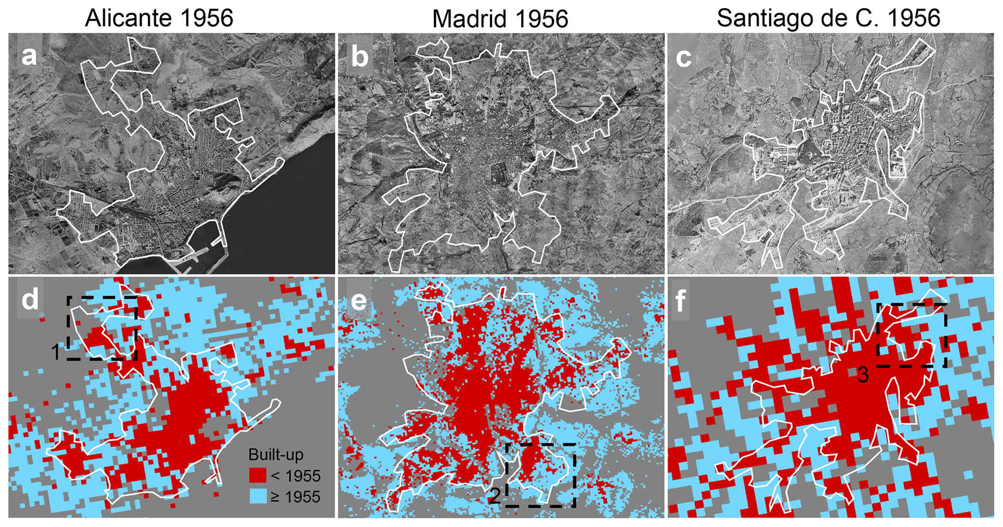
Figure 17Visual comparison of HISDAC-ES to aerial imagery from 1956. Aerial image overlaid with manually digitized urban extents for (a) Alicante, (b) Madrid, and (c) Santiago de Compostela and (d)–(f) overlaid with the HISDAC-ES built-up grid cells after and prior to 1955. Dashed black boxes are selected areas of discrepancies (i.e., turquoise areas within the digitized urban boundaries or red areas without the urban boundary), which are enlarged and discussed in the Appendix Fig. A6.
4.6 Attribute completeness and coverage
Lastly, we report the INSPIRE building attribute completeness at the municipality level, compared to the total number of buildings available in each municipality (Fig. 18a). We observe very high levels of completeness of the construction year attribute (Fig. 18b). The building function attribute has a high coverage, except in the Gipuzkoa and Bizkaia provinces on the northern coast (Fig. 18c). Moreover, there is a building function attribute, “other”, that is only available in the Navarre region, which we excluded from the HISDAC-ES dataset (Fig. 18d). Thus, the uncertainty in the (historical) land use layers in HISDAC-ES in Navarre is slightly higher, as it is unknown what building function the “other” class encompasses. The indoor area, number of dwellings, and number of building units attributes also have lower levels of completeness in some areas of the Basque Country (Fig. 18e, f, h).The completeness of “number of dwellings” is higher in buildings labeled as “residential” (Fig. 18g) than across all buildings (Fig. 18f), as this attribute is semantically linked to (mostly) residentially used buildings. Conversely, information on the number of floors is highly complete in the Navarre region (Fig. 18j) but otherwise not covered in the remaining provinces and, thus, has not been used in this version of HISDAC-ES.
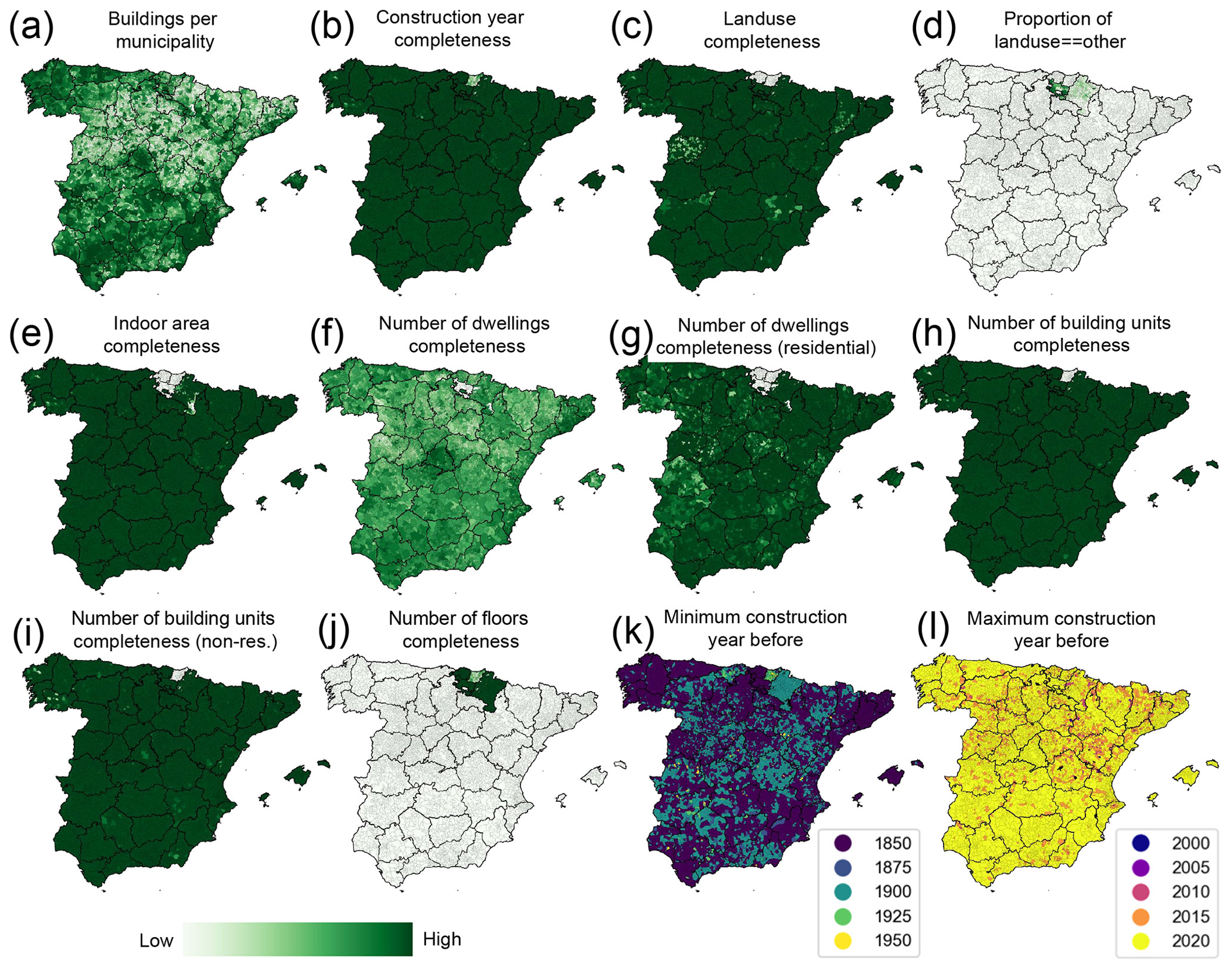
Figure 18Attribute completeness and construction year coverage at the municipality level. See the Appendix Fig. G1 for corresponding maps of the Canary Islands.
We also assessed the temporal coverage of construction year information at the municipality level, in order to better understand potential survivorship bias in the data. As can be seen in Fig. 18k, most municipalities have the earliest construction year on record <1850 or <1900. Only a few regions have minimum construction years between 1900 and 1925 (e.g., regions around San Sebastián and Bilbao), whereas very few, scattered municipalities have earliest construction years between 1925 and 1950. In these municipalities, data users should be careful when conducting long-term analyses, as survivorship bias may be high. Likewise, we mapped out the maximum construction year per municipality (Fig. 18l), indicating the recentness of the cadastral building data underlying HISDAC-ES, as in most municipalities, the most recent construction year on record is between 2015 and 2020. Generally, these high levels of attribute completeness and temporal coverage are encouraging and indicate that the layers derived from these attributes are expected to be highly reliable at least for recent points in time. We made these municipality-level attribute completeness statistics available in the data repository.
All datasets are available at https://doi.org/10.6084/m9.figshare.22009643 (Uhl et al., 2023a). All raster datasets are available in Lempel–Ziv–Welch (LZW)-compressed GeoTIFF format and have a spatial resolution of 100 m × 100 m. All raster datasets are available in EPSG:3035 (LAEA, all Spanish territory), EPSG:4083 (REGCAN, Canary Islands), and EPSG:25830 (UTM30N, Iberian Peninsula) projections. The raster datasets are organized in subfolders as follows: they are grouped by geographic coverage (all, can, ibe) and reference system (laea, regcan, utm) and by theme (evolution, landuse, physical, temporal). For example, “ibe_utm_age” contains the layers measuring age-related characteristics of the built environment, covering the Iberian Peninsula, referenced to the UTM grid (see Table 5). In total, there are 743 GeoTIFF files. Municipality-level aggregates and uncertainty measures are available in CSV format and in GeoPackage (.gpkg) format (EPSG:3035) including municipality boundaries, obtained from https://doi.org/10.7419/162.09.2020 (Centro Nacional de Información Geográfica, 2023) (recintos_municipales_inspire_peninbal_etrs89.shp, recintos_municipales_inspire_canarias_regcan95.shp). The data in the repository are partitioned into four ZIP-compressed archives, one for the raster data in each of the three spatial reference systems and one for the municipality-level aggregates. For reproducibility purposes, the building footprint centroids derived from the cadastral data (downloaded in June 2021) are also made available as geospatial vector data in GeoPackage format.
The Python code used to create HISDAC-ES (i.e., input vector data, raster data, municipality-level data) is publicly available at https://github.com/johannesuhl/hisdac-es (last access: 13 October 2023) (https://doi.org/10.5281/zenodo.8429118, Uhl, 2023). R users can access the Spanish cadastral data underlying HISDAC-ES using the CatastRo package, which is available at (https://ropenspain.github.io/CatastRo/index.html, last access: 13 October 2023) (https://doi.org/10.5281/zenodo.6044091, Delgado Panadero and Hernangómez, 2023), as well as the CatastRoNav package (for cadastral data from Navarre; https://ropenspain.github.io/CatastRoNav/, last access: 11 October 2023; https://doi.org/10.5281/zenodo.6366407, Hernangómez, 2023), and comprehensive instructions for building age visualization in R can be found at https://dominicroye.github.io/en/2019/visualize-urban-growth/ (Royé, 2019).
In this “Data description” paper, we presented the creation and characteristics of HISDAC-ES, a set of geospatial raster and vector layers measuring the built environment in Spain from different perspectives, including physical, temporal, evolutionary, and functional aspects. HISDAC-ES aims to (a) facilitate the access to and use of information derived from cadastral building data by spatial, temporal, and semantic aggregation; (b) provide empirically measured, historical geospatial data, enabling contemporary but also long-term, historical analyses of urban growth, sprawl, and change; and (c) demonstrate the usefulness of cadastral data for geographic applications in general and domains of social and environmental sciences, more specifically. HISDAC-ES represents an extension of related work, recently conducted on US property data (HISDAC-US; Leyk and Uhl, 2018; Uhl et al., 2021c; McShane et al., 2022), and demonstrates the benefit of open data policies and large-scale data harmonization efforts for the scientific community and beyond.
HISDAC-ES provides a valuable data source for urban analysts, regional planners, and policy makers, enabling or upscaling the quantitative measurement and interpretation of long-term urbanization and land development processes (e.g., Arribas-Bel et al., 2011; Alvarez-Palau et al., 2019; Sapena and Ruiz, 2019; Zornoza-Gallego 2022b; Domingo et al., 2023). Together with the sister product HISDAC-US, it will enable the comparative study of urban size, shape, and morphology over long time periods, across different continents, and across historical as well as cultural settings.
We evaluated the agreement of HISDAC-ES with a range of related datasets obtained from remote sensing data and historical maps, identifying varying levels of agreement. While the associations between datasets imply some level of coherence and are generally promising, it is important to point out that a rigorous quality assessment of historical geospatial data is difficult. The main reasons are the general lack of reliable, historical reference data but also differences in definitions and semantic discrepancies (ambiguity) between the evaluation datasets and HISDAC-ES, as well as vagueness in the evaluation datasets (e.g., arbitrarily defined urban boundaries).
Nonetheless, there are a few shortcomings of HISDAC-ES that need to be addressed in the future. The main issue is the survivorship bias in the data: we infer settlement age based on the construction year on record in the cadastral building data. It remains unknown whether a construction date represents the first establishment of a building at a given location or whether there was a built-up structure existing prior to that. Similarly, buildings that existed in the past, but have been demolished, are not contained in HISDAC-ES. Thus, HISDAC-ES can only measure urban growth but not urban shrinkage or urban renewal. Fortunately, the latter process is rare. It is also unknown if the different attributes in the cadastral building data underlying the HISDAC-ES were measured at the same time. For example, the building function and indoor area, etc., reflect the contemporary state of a building (i.e., as of the year 2020), but these properties may have changed since the construction year on record, which may introduce additional uncertainty in the evolutionary layers in HISDAC-ES. Moreover, missing attributes in the cadastral data underlying HISDAC-ES could be estimated using specific data imputation strategies (e.g., Milojevic-Dupont et al., 2020). The complementary nature of certain, related building attributes (such as building indoor area, building height, number of floors, building volume, and average floor height) could also be exploited for such data imputation efforts (see Fig. 18).
Importantly, as the cadastral data used to create HISDAC-ES originate from different cadastral systems, there may be inconsistencies in the definition and in the measurement of specific attributes. For example, the way that building indoor area (BIA) is defined and measured could vary across the different cadastral systems, despite conforming to the specifications of the INSPIRE directive aiming to homogenize cadastral data across the EU. Also, the definition and measurement of building units or number of dwellings could be affected by such inconsistencies, where the building footprint area (the input data for the BUFA layers) can be expected to be least affected by differences in cadastral systems. Thus, future work needs to thoroughly assess (and account for) such potential inconsistencies between the different cadastral systems. Similarly, the variables DWEL (number of dwellings) and BUNITS (building units) need to be treated carefully, due to their potential semantic overlap: for example, while DWEL only contains residential units, BUNITS may contain both residentially and non-residentially used building units, for example, in the case of buildings of mixed use. Generally, we advise to be cautious when employing the HISDAC-ES data layers for demographic modeling applications, where the propagation of uncertainty from the input data to the outputted products needs to be taken into account (e.g., Goerlich-Gisbert and Cantarino-Marti, 2017). Finally, the gridded surfaces in HISDAC-ES are based on discrete point locations, rather than the actual building footprint geometries, in order to reduce computational processing effort. Thus, large buildings extending across two or more grid cells may not be represented correctly in HISDAC-US, introducing some positional uncertainty in the data. For this reason, grid cell values in the BUFA layers (representing the built-up area per cell) may exceed the grid cell area in some cases.
Future work should focus on validation of the HISDAC-ES dataset, for example, by employing large-scale historical map collections (cf. Olazabal et al., 2019) or other historical records. The integration of HISDAC-ES with historical population data in a dasymetric modeling framework could be useful to create fine-grained, historical population estimates (cf. Silveira et al., 2013; Burghardt et al., 2022b). Moreover, other components of Spanish cadastral building data could be used, such as sub-building-level information (e.g., building parts), to create fine-grained data on building function at the sub-building level, and information on building heights, which is available in a separate data pool (https://www.catastro.minhap.es/webinspire/documentos/Conjuntos de datos.pdf, last access: 11 October 2023). Lastly, with the prospect of increasing availability of INSPIRE-conforming cadastral building data, HISDAC-related efforts will be expanded to other European countries where cadastral building data are of similarly high completeness, quality, and thematic richness.
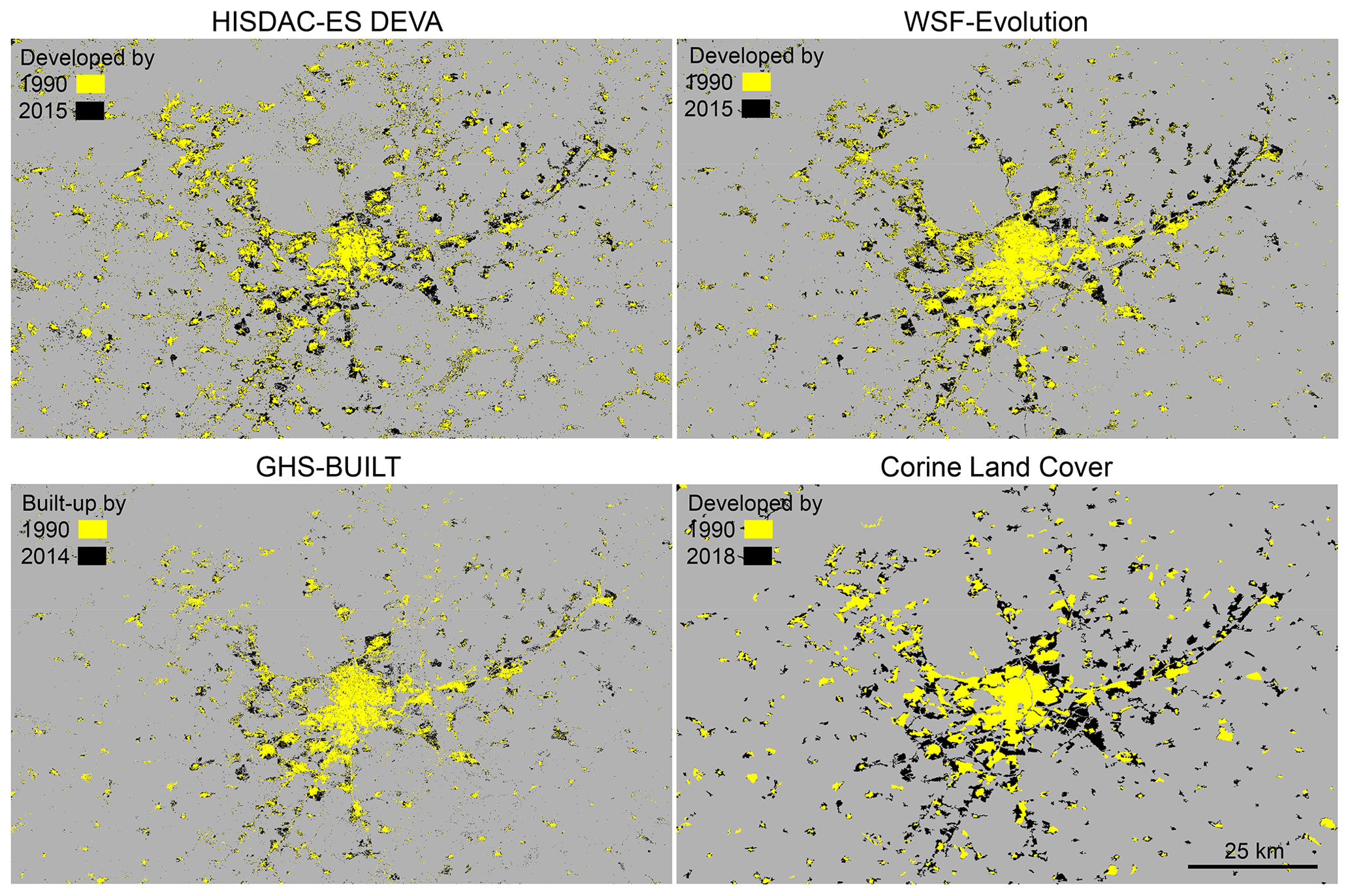
Figure A1Visual comparison of HISDAC-ES DEVA, WSF-Evolution, GHS-BUILT, and CORINE Land Cover, in 1990 and approximately 2015. For CORINE Land Cover, only the classes “continuous urban fabric”, “discontinuous urban fabric”, “industrial or commercial units”, “sport and leisure facilities”, “construction sites”, and “port areas” are shown, which are loosely related to developed/built-up areas.
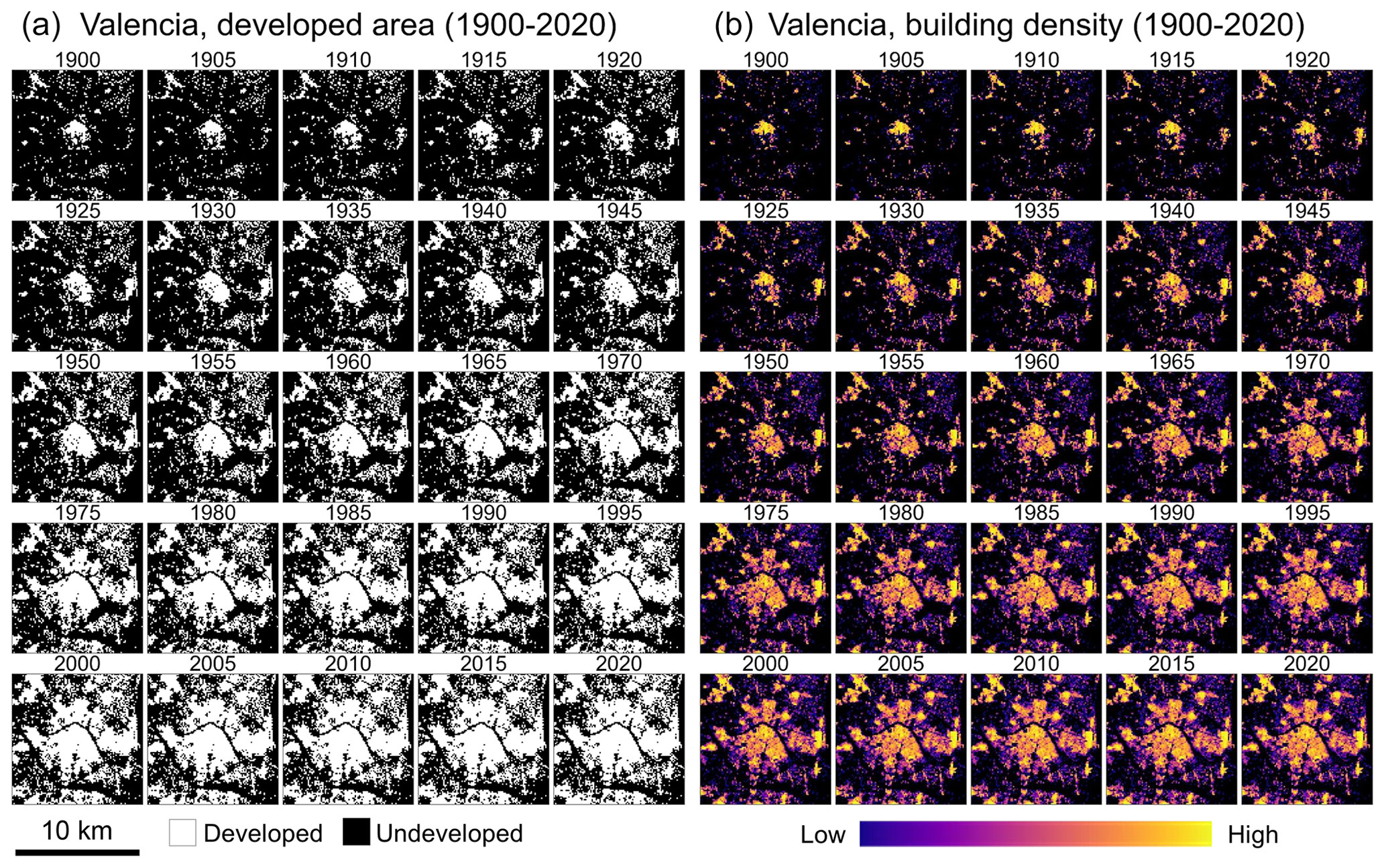
Figure B1Complete time series of the DEVA (developed area, a) and BUDENS (building density, b) raster time series in 5-year intervals from 1900 to 2020. Data shown for the city of Valencia.
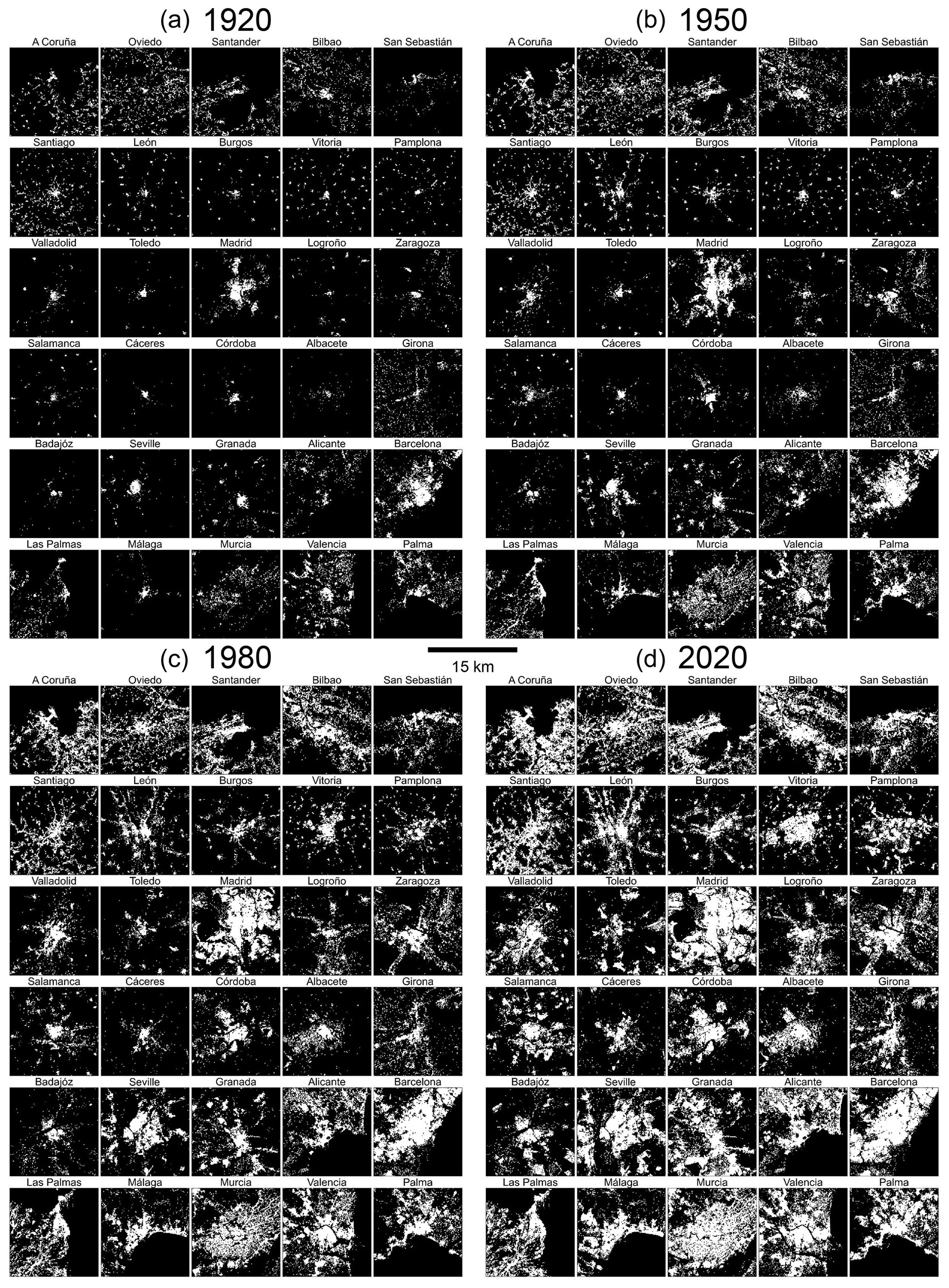
Figure B2HISDAC-ES developed area layers (DEVA) for (a) 1920, (b) 1950, (c) 1980, and (d) 2020 for a selection of 30 cities in Spain. Cities are arranged in an approximate, quasi-geographic space (San Sebastián in the upper right is located in the northeast, and Las Palmas in the lower left is located in the southwest.

Figure C1Exemplary municipality-level aggregates for the Canary Islands in 1900, 1960, and 2020.
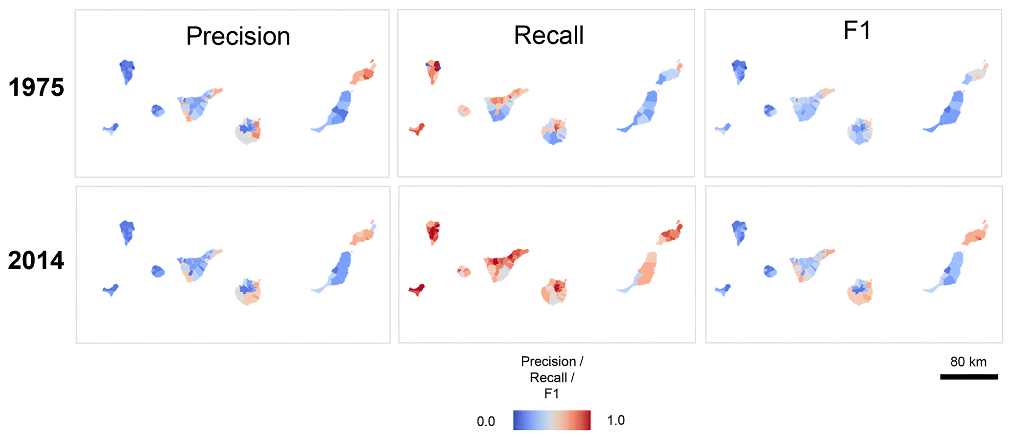
Figure D1Municipality-level agreement of HISDAC-ES DEVA and GHS-BUILT R2018A for the Canary Islands.
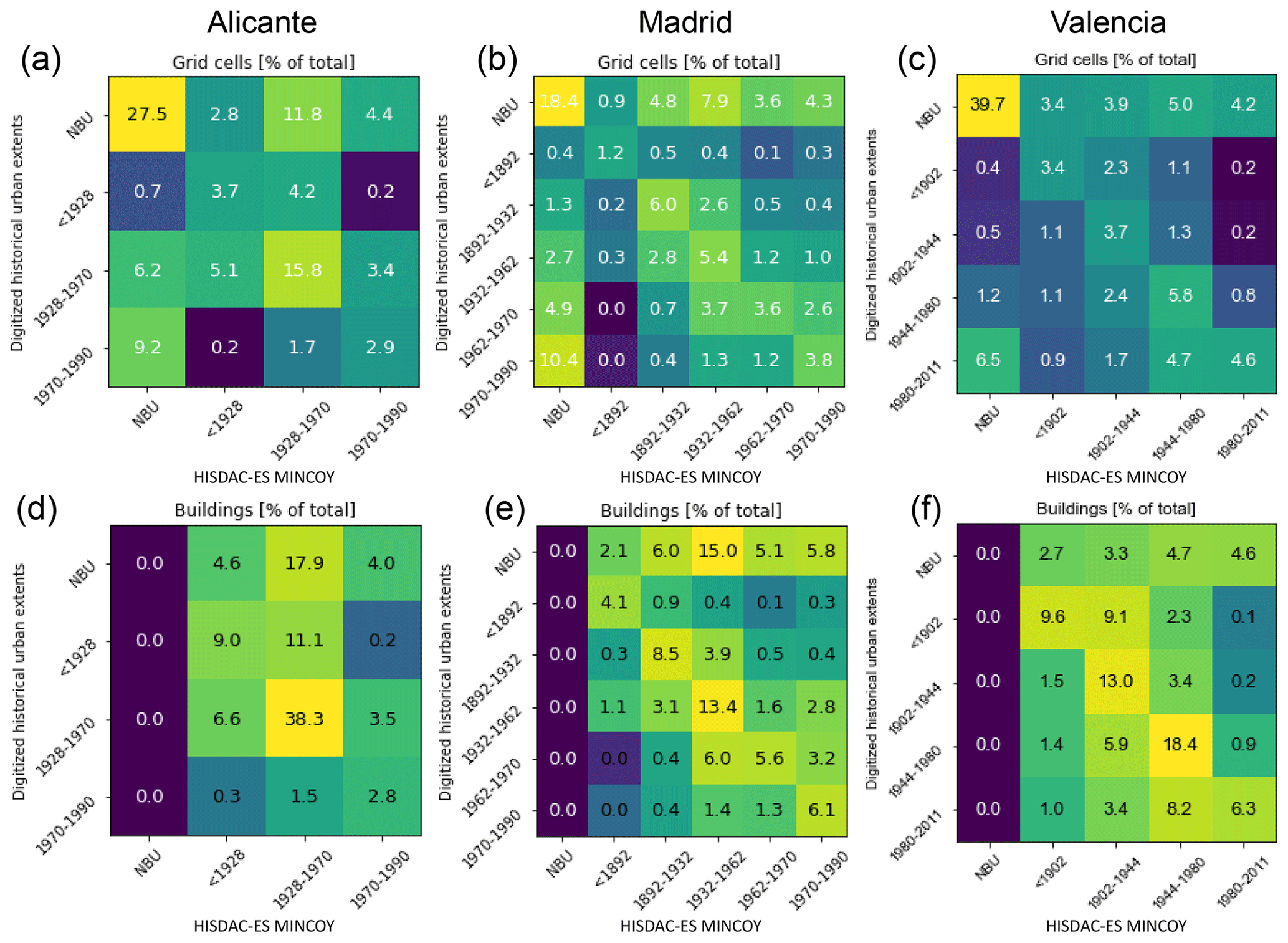
Figure E1Confusion matrices underlying Table 4 from map comparison of the MINCOY and urban extents digitized from historical maps for (a) Alicante, (b) Madrid, and (c) Valencia. While panels (a)–(c) cross-tabulate the grid cell counts in each category, panels (d)–(f) are based on the number of buildings reported in HISDAC-ES within each category.
-
Alicante: Alférez Rojas Navarrete Barracks. Even though this military facility existed in 1955, it is not well covered in the cadastral data underlying the HISDAC-ES. Despite covering a large area, it is only represented by one grid cell in the HISDAC-ES layers for 1955. It is likely that military facilities were not mapped the same way as regular residential neighborhoods, possibly for security reasons.
-
Madrid: Housing colonies Entrevías (Vallecas II). This large social housing colony was completely renewed at a later point in time. This is an extreme example of urban renewal, which cannot be measured by the HISDAC-ES data.
-
Santiago de Compostela. This discrepancy between the HISDAC-ES data and the manually drawn urban boundary is due to a definitional problem. In the aerial image of the Monte da Almáciga region, the large building complex is a college, surrounded by scattered settlements, possibly of agricultural usage. In this case, we excluded these areas from the “urban extent” due to the low settlement density, even though these areas should be considered “urban” due to their functional importance. This definitional mismatch causes this discrepancy.
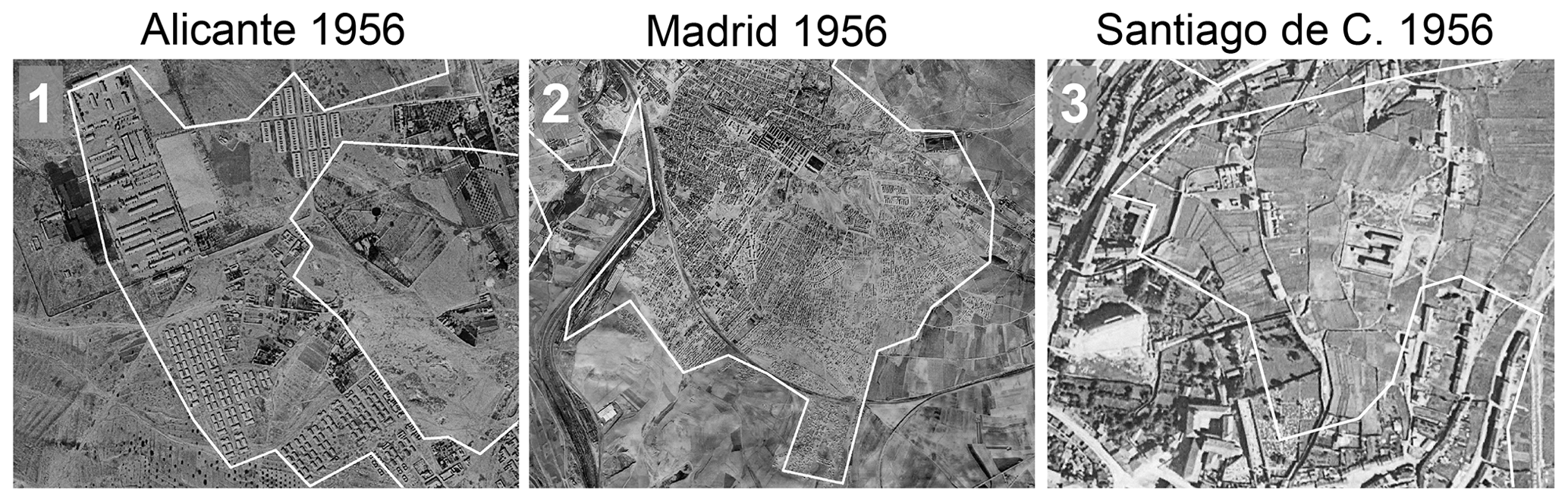
Figure F1Examples of discrepancies between HISDAC-ES and the 1956 aerial imagery. Shown are three regions highlighted in Fig. 17.
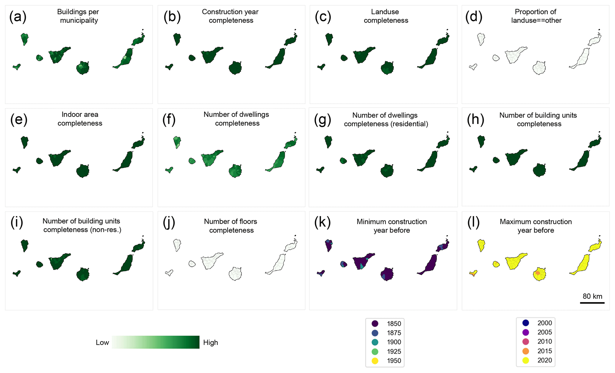
Figure G1Attribute completeness and temporal coverage at the municipality level for the Canary Islands.
We provide eight animated data visualizations (available at https://doi.org/10.6084/m9.figshare.22064798, Uhl et al., 2023b), showcasing several data layers of the HISDAC-ES, at the grid cell level and at the municipality level:
-
evolution of developed areas (DEVA) in 30 urban centers in Spain (01_hisdac_es_developed_area_evolution.gif),
-
evolution of building density (BUDENS) in 30 urban centers in Spain (02_hisdac_es_building_density_evolution.gif),
-
evolution of building footprint area (BUFA) in 30 urban centers in Spain (03_hisdac_es_building_footprint_area_evolution.gif),
-
evolution of residential land use in 30 urban centers in Spain (04_hisdac_es_residential_landuse_evolution.gif),
-
evolution of commercial land use in 30 urban centers in Spain (05_hisdac_es_commercial_landuse_evolution.gif),
-
evolution of industrial land use in 30 urban centers in Spain (06_hisdac_es_industrial_landuse_evolution.gif),
-
evolution of building footprint area (BUFA) per municipality (07_hisdac_es_municipality_bufa_density.gif),
-
evolution of building density (BUDENS) per municipality (08_hisdac_es_municipality_building_density.gif).
Animations 1–3 are shown from 1920 to 2020. Animations 4–6 are shown from 1950 to 2020. Note that for the land-use-related animations (4–6), we binarized the building density layers stratified by land use category (i.e., highlighting grid cells where at least one building of the respective land use class exists). Major cities where no land use information was available (i.e., San Sebastián and Bilbao, shown in animations 1–3) were replaced by the cities of Cadiz and Jaén in animations 4–6. Animations 7 and 8 show the municipality-level aggregates, converted into densities (i.e., built-up area per square kilometer and buildings per square kilometer), shown in percentiles based on the data distributions across all years.
The supplement related to this article is available online at: https://doi.org/10.5194/essd-15-4713-2023-supplement.
JHU, DR, and SL designed the data model. JHU and DR acquired the source data. DR, MBS, JAAV, and JHU gathered evaluation data. JHU implemented the code for data production. JHU, DR, SL, and KB designed the evaluation experiments. JHU implemented and carried out the data production process and the evaluation analyses. JHU and DR visualized the results. JHU prepared the manuscript with contributions from all co-authors.
The contact author has declared that none of the authors has any competing interests.
The content is solely the responsibility of the authors and does not necessarily represent the official views of National Institutes of Health (NIH) or University of Colorado Population Center (CUPC).
Publisher’s note: Copernicus Publications remains neutral with regard to jurisdictional claims in published maps and institutional affiliations.
Thanks are given to Carmen Zornoza-Gallego for providing data on historical urban extents for the city of Valencia, used for the evaluation studies presented herein. Partial funding for this work was provided through the Humans, Disasters, and the Built Environment and the Human Networks and Data Science – Infrastructure programs of the US National Science Foundation (award numbers 1924670 and 2121976, respectively) to the University of Colorado Boulder. Moreover, this research benefited from support provided to the University of Colorado Population Center (CUPC; project 2P2CHD066613-06) from the Eunice Kennedy Shriver National Institute of Child Health and Human Development. Moreover, this study was supported partially by the Open Philanthropy Project. Keith Burghardt was funded in part by the Defense Advanced Research Projects Agency (DARPA) and Army Research Office (ARO) under contract no. W911NF-21-C-0002. Finally, this work was supported, in part, by HE ICARIA project (HORIZON-MISS-2021-CLIMA-02-03, grant ID: 101093806 ICARIA).
This research has been supported by the Eunice Kennedy Shriver National Institute of Child Health and Human Development (grant no. 2P2CHD066613-06), the National Science Foundation (grant nos. 2121976 and 1924670), the Open Philanthropy Project (grant no. 1433), the Defense Advanced Research Projects Agency (grant no. W911NF-21-C-0002), and the HE ICARIA project (grant no. 101093806 ICARIA).
This paper was edited by David Carlson and reviewed by Tracy Kugler and two anonymous referees.
Alonso, W.: The historic and the structural theories of urban form: Their implications for urban renewal, Land Econ., 40, 227–231, 1964.
Alvarez-Palau, E. J., Martí-Henneberg, J., and Solanas-Jiménez, J.: Urban Growth and Long-Term Transformations in Spanish Cities Since the Mid-Nineteenth Century: A Methodology to Determine Changes in Urban Density, Sustainability, 11, 6948, https://doi.org/10.3390/su11246948, 2019.
Arribas-Bel, D., Nijkamp, P., and Scholten, H.: Multidimensional urban sprawl in Europe: A self-organizing map approach, Comput. Environ. Urban. Syst., 35, 263–275, 2011.
Atwal, K. S., Anderson, T., Pfoser, D., and Züfle, A.: Predicting building types using OpenStreetMap, Scientific Reports, 12, 19976, https://doi.org/10.1038/s41598-022-24263-w, 2022.
Balch, J. K., Iglesias, V., Braswell, A. E., Rossi, M. W., Joseph, M. B., Mahood, A. L., Shrum, T. R., White, C. T., Scholl, V. M., McGuire, B., Karban, C., Buckland, M., and Travis, W. R.: Social-environmental extremes: Rethinking extraordinary events as outcomes of interacting biophysical and social systems, Earth's Future, 8, e2019EF001319, https://doi.org/10.1029/2019EF001319, 2020.
Bernard, L., Kanellopoulos, I., Annoni, A., and Smits, P.: The European geoportal – one step towards the establishment of a European Spatial Data Infrastructure, Comput. Environ. Urban. Syst., 29, 15–31, 2005.
Boeing, G.: Off the grid … and back again? The recent evolution of American street network planning and design, J. Am. Plann. Assoc., 87, 123–137, 2021.
Braswell, A. E., Leyk, S., Connor, D. S., and Uhl, J. H.: Creeping disaster along the US coastline: Understanding exposure to sea level rise and hurricanes through historical development, PLoS one, 17, e0269741, https://doi.org/10.1371/journal.pone.0269741, 2022.
Burghardt, K., Uhl, J. H., Lerman, K., and Leyk, S.: Road network evolution in the urban and rural United States since 1900, Comput. Environ. Urban. Syst., 95, 101803, https://doi.org/10.1016/j.compenvurbsys.2022.101803, 2022a.
Burghardt, K., Uhl, J. H., Lerman, K., and Leyk, S.: Analyzing urban scaling laws in the United States over 115 years, arXiv [preprint], https://doi.org/10.48550/arXiv.2209.10852, 22 September 2022b.
Büttner, G.: CORINE land cover and land cover change products, in: Land use and land cover mapping in Europe: practices & trends, 55–74, Dordrecht, Springer Netherlands, ISBN 978-94-007-7969-3, https://doi.org/10.1007/978-94-007-7969-3, 2014.
Büttner, G., Kosztra, B., Maucha, G., Pataki, R., Kleeschulte, S., Hazeu, G. W., Vittek, M., Schröder, C., and Littkopf, A.: Copernicus Land Monitoring Service – CORINE Land Cover, User Manual, Copernicus Publications, https://land.copernicus.eu/en/technical-library/clc-product-user-manual/@@download/file (last access: 13 October 2023), 2021.
Centro Nacional de Información Geográfica: Centro de Descargas, Centro Nacional de Información Geográfica [data set], https://doi.org/10.7419/162.09.2020, 2023.
Cetl, V., de Lima, V. N., Tomas, R., Lutz, M., D'Eugenio, J., Nagy, A., and Robbrecht J.: Summary report on status of implementation of the INSPIRE directive in EU, JRC Technical Report, https://doi.org/10.2760/143502, 2017.
Connor, D. S., Gutmann, M. P., Cunningham, A. R., Clement, K. K., and Leyk, S.: How entrenched is the spatial structure of inequality in cities? Evidence from the integration of census and housing data for Denver from 1940 to 2016, Ann. Am. Assoc. Geogr., 110, 1022–1039, 2020.
Delgado Panadero, Á. and Hernangómez, D.: CatastRo: Interface to the API Sede Electrónica Del Catastro, Zenodo [code], https://doi.org/10.5281/zenodo.6044091, 2023.
Demuzere, M., Bechtel, B., Middel, A., and Mills, G.: Mapping Europe into local climate zones, PloS One, 14, e0214474, https://doi.org/10.1371/journal.pone.0214474, 2019.
Diaz-Pacheco, J. and Gutiérrez, J.: Exploring the limitations of CORINE Land Cover for monitoring urban land-use dynamics in metropolitan areas, J. Land Use Sci., 9, 243–259, 2014.
Domingo, D., Van Vliet, J., and Hersperger, A. M.: Long-term changes in 3D urban form in four Spanish cities, Landsc. Urban Plan., 230, 104624, https://doi.org/10.1016/j.landurbplan.2022.104624, 2023.
Dornbierer, J., Wika, S., Robison, C., Rouze, G., and Sohl, T.: Prototyping a methodology for long-term (1680–2100) historical-to-future landscape modeling for the conterminous United States, Land, 10, 536, https://doi.org/10.3390/land10050536, 2021.
Esch, T., Brzoska, E., Dech, S., Leutner, B., Palacios-Lopez, D., Metz-Marconcini, A., Marconcini, M., Roth, A., and Zeidler, J.: World Settlement Footprint 3D-A first three-dimensional survey of the global building stock, Remote Sens. Environ., 270, 112877, https://doi.org/10.1016/j.rse.2021.112877, 2022.
European Union: Directive (EU) 2019/1024 of the European Parliament and of the Council of 20 June 2019 on open data and the re-use of public sector information, in OJ L 172, 26.6.2019, 56–83, ELI http://data.europa.eu/eli/dir/2019/1024/oj (last access: 11 October 2023), 2019.
Ewing, R. and Rong, F.: The impact of urban form on US residential energy use, Housing policy debate, 19, 1–30, https://doi.org/10.1080/10511482.2008.9521624, 2008.
Ferrara, A., Testa, P., and Zhou, L.: New area-and population-based geographic crosswalks for US counties and congressional districts, 1790-2020, SSRN 4019521, https://doi.org/10.2139/ssrn.4019521, 2021.
Florczyk, A. J., Corbane, C., Ehrlich, D., Freire, S., Kemper, T., Maffenini, L., Melchiorri, M., Pesaresi, M., Politis, P., Schiavina, M. and Sabo, F.: GHSL data package 2019, Luxembourg, EUR, 29788(10.2760), p. 290498, https://doi.org/10.2760/290498, 2019.
Goerlich-Gisbert, F. J. and Cantarino-Marti, I.: Grid poblacional 2011 para España. Evaluación metodológica de diversas posibilidades de elaboración, Estud. Geogr., 78, 135–163, 2017.
Gong, P., Li, X., Wang, J., Bai, Y., Chen, B., Hu, T., Liu, X., Xu, B., Yang, J., Zhang, W., and Zhou, Y.: Annual maps of global artificial impervious area (GAIA) between 1985 and 2018, Remote Sens. Environ., 236, 111510, https://doi.org/10.1016/j.rse.2019.111510, 2020.
Gröger, G. and Plümer, L.: The interoperable building model of the European Union, in: Geoinformation for Informed Decisions, Springer, Cham, 1–17, https://doi.org/10.1007/978-3-319-03644-1, 2014.
Haberl, H., Wiedenhofer, D., Schug, F., Frantz, D., Virág, D., Plutzar, C., Gruhler, K., Lederer, J., Schiller, G., Fishman, T., and Lanau, M.: High-resolution maps of material stocks in buildings and infrastructures in Austria and Germany, Environ. Sci. Technol., 55, 3368–3379, 2021.
Hernangómez, D.: CatastRoNav: Interface to the API Catastro de Navarra, Zenodo [code], https://doi.org/10.5281/zenodo.6366407, 2023.
Hudson, P.: Urban Characterisation; Expanding Applications for, and New Approaches to Building Attribute Data Capture, Hist. Environ. Policy, 9, 306–327, https://doi.org/10.1080/17567505.2018.1542776, 2018.
IBM: Atom feed format, https://www.ibm.com/docs/en/baw/19.x?topic=formats-atom-feed-format, last access: 11 October 2023.
Iglesias, V., Braswell, A. E., Rossi, M. W., Joseph, M. B., McShane, C., Cattau, M., Koontz, M. J., McGlinchy, J., Nagy, R. C., Balch, J., Leyk, S., and Travis, W. R.: Risky development: Increasing exposure to natural hazards in the United States, Earth's Future, 9, e2020EF001795, https://doi.org/10.1029/2020EF001795, 2021.
Instituto Nacional de Geografía: Planimetría historical maps Web Map Service, Online resource, http://www.ign.es/wms/minutas-cartograficas?request=GetCapabilities&service=WMS& (last access: 10 October 2023), 2022.
Klein Goldewijk, C. G. M.: Anthropogenic land-use estimates for the Holocene; HYDE 3.2, DANS Data Station Archaeology [data set], https://doi.org/10.17026/dans-25g-gez3, 2017.
Klein Goldewijk, K. and Verburg, P. H.: Uncertainties in global-scale reconstructions of historical land use: an illustration using the HYDE data set, Landsc. Ecol., 28, 861–877, 2013.
Klein Goldewijk, K., Beusen, A., Doelman, J., and Stehfest, E.: Anthropogenic land use estimates for the Holocene – HYDE 3.2, Earth Syst. Sci. Data, 9, 927–953, https://doi.org/10.5194/essd-9-927-2017, 2017.
Leyk, S. and Uhl, J. H.: HISDAC-US, historical settlement data compilation for the conterminous United States over 200 years, Sci. Data, 5, 180175, https://doi.org/10.1038/sdata.2018.175, 2018.
Leyk, S., Ruther, M., Buttenfield, B. P., Nagle, N. N., and Stum, A. K.: Modeling residential developed land in rural areas: A size-restricted approach using parcel data, Appl. Geog., 47, 33–45, 2014.
Leyk, S., Uhl, J. H., Balk, D., and Jones, B.: Assessing the accuracy of multi-temporal built-up land layers across rural-urban trajectories in the United States, Remote Sens. Environ., 204, 898–917, 2018.
Leyk, S., Uhl, J. H., Connor, D. S., Braswell, A. E., Mietkiewicz, N., Balch, J. K., and Gutmann, M.: Two centuries of settlement and urban development in the United States, Sci. Adv., 6, eaba2937, https://doi.org/10.1126/sciadv.aba2937, 2020.
Li, M., Wang, Y., Rosier, J. F., Verburg, P. H., and van Vliet, J.: Global maps of 3D built-up patterns for urban morphological analysis, Int. J. Appl. Earth. Obs. Geoinf., 114, 103048, https://doi.org/10.1016/j.jag.2022.103048, 2022.
Li, X., Zhou, Y., Hejazi, M., Wise, M., Vernon, C., Iyer, G., and Chen, W.: Global urban growth between 1870 and 2100 from integrated high resolution mapped data and urban dynamic modelling, Commun. Earth Env., 2, 201, https://doi.org/10.1038/s43247-021-00273-w, 2021.
Liu, F., Wang, S., Xu, Y., Ying, Q., Yang, F., and Qin, Y.: Accuracy assessment of Global Human Settlement Layer (GHSL) built-up products over China, PLoS One, 15, e0233164, https://doi.org/10.1371/journal.pone.0233164, 2020.
Marconcini, M., Gorelick, N., Metz-Marconcini, A., and Esch, T.: Accurately monitoring urbanization at global scale–the world settlement footprint, IOP Conf. Ser.: Earth Environ. Sci., 509, 012036, https://doi.org/10.1088/1755-1315/509/1/012036, 2020a.
Marconcini, M., Metz-Marconcini, A., Üreyen, S., Palacios-Lopez, D., Hanke, W., Bachofer, F., Zeidler, J., Esch, T., Gorelick, N., Kakarla, A., Paganini, M., and Strano, E.: Outlining where humans live, the World Settlement Footprint 2015, Sci. Data, 7, 242, https://doi.org/10.1038/s41597-020-00580-5, 2020b.
McDonald, R. I., Biswas, T., Sachar, C., Housman, I., Boucher, T. M., Balk, D., Nowak, D., Spotswood, E., Stanley, C. K., and Leyk, S.: The tree cover and temperature disparity in US urbanized areas: Quantifying the association with income across 5723 communities, PloS one, 16, e0249715, https://doi.org/10.1371/journal.pone.0249715, 2021.
McShane, C., Uhl, J. H., and Leyk, S.: Gridded land use data for the conterminous United States 1940–2015, Sci. Data, 9, 493, https://doi.org/10.1038/s41597-022-01591-0, 2022.
Mietkiewicz, N., Balch, J. K., Schoennagel, T., Leyk, S., St. Denis, L. A., and Bradley, B. A.: In the line of fire: consequences of human-ignited wildfires to homes in the US (1992–2015), Fire, 3, 50, https://doi.org/10.3390/fire3030050, 2020.
Millard-Ball, A.: The width and value of residential streets, J. Am. Plann. Assoc., 88, 30–43, 2022.
Millhouser, P.: Evaluating Landscape Connectivity and Habitat Fragmentation Effects on Elk in the Roaring Fork and Eagle Valleys, Master's Thesis, Pennsylvania State University, https://www.researchgate.net/publication/335106926_Evaluating_Landscape_Connectivity_and_Habitat_Fragmentation_Effects_on_Elk_in_the_Roaring_Fork_and_Eagle_Valleys (last access: 13 October 2023), 2019.
Milojevic-Dupont, N., Hans, N., Kaack, L. H., Zumwald, M., Andrieux, F., de Barros Soares, D., Lohrey, S., Pichler, P. P., and Creutzig, F.: Learning from urban form to predict building heights, PLoS One, 15, e0242010, https://doi.org/10.1371/journal.pone.0242010, 2020.
Milojevic-Dupont, N., Wagner, F., Nachtigall, F., Hu, J., Brüser, G. B., Zumwald, M., Biljecki, F., Heeren, N., Kaack, L. H., Pichler, P. P. and Creutzig, F.: EUBUCCO v0.1: European building stock characteristics in a common and open database for 200+ million individual buildings, Sci. Data, 10, 147, https://doi.org/10.1038/s41597-023-02040-2, 2023.
Minghini, M., Cetl, V., Kotsev, A., Tomas, R., and Lutz, M.: INSPIRE: The entry point to Europe's big geospatial data infrastructure, in: Handbook of Big Geospatial Data, Springer, Cham, 619–641, https://doi.org/10.1007/978-3-030-55462-0, 2021.
Miranda, A. S.: The micro persistence of layouts and design: quasi-experimental evidence from the United States housing corporation, Reg. Sci. Urb. Econ., 95, 103755, https://doi.org/10.1016/j.regsciurbeco.2021.103755, 2022.
Nolte, C.: High-resolution land value maps reveal underestimation of conservation costs in the United States, P. Natl. Acad. Sci. USA, 117, 29577–29583, 2020.
Nolte, C., Boyle, K. J., Chaudhry, A., Clapp, C., Guignet, D., Hennighausen, H., Kushner, I., Liao, Y., Mamun, S., Pollack, A., Richardson, J., Sundquist, S., Swedberg, K., and Uhl, J. H.: Data Practices for Studying the Impacts of Environmental Amenities and Hazards with Nationwide Property Data, Land Econ., Jun 2023, 102122-0090R, https://doi.org/10.3368/le.100.1.102122-0090R, 2023.
Olazabal, E., Alvarez Palau, E., Barquín, R., Macías Muñoz, M. O., Martí Henneberg, J., Morillas-Torné, M., Ortúñez, P. P., and Solanas, J.: Catálogo digital de cartografía urbana contemporánea en España (1800–1950), Biblio 3W, Revista Electrónica Bibliográfica de Geografía y Ciencias Sociales Universidad de Barcelona, 2019, vol. XXIV, 1267, https://revistes.ub.edu/index.php/b3w/article/view/27944 (last access: 11 October 2023), 2019.
Pesaresi, M., Corbane, C., Ren, C., and Edward, N.: Generalized Vertical Components of built-up areas from global Digital Elevation Models by multi-scale linear regression modelling, PLoS One, 16, e0244478, https://doi.org/10.1371/journal.pone.0244478, 2021.
Remírez, P., Martínez de Marigorta, M. Á., Fragua, R., Izquierdo, M., LLinàs, J., Lorenzo, E., and Más, R. M.: GradualMap, SL, Rugoma SA, RevisaAtlas SA, Técnica Cartográfica Andaluza SA, Digraf SL, and Tracasa SA: Gran atlas de España Planeta (Segunda), Editorial Planeta, S.A., ISBN 9788408462491, 1998.
Royé, D.: Visualize urban growth, GitHub [code], https://dominicroye.github.io/en/2019/visualize-urban-growth/ (last access: 11 October 2023), 2019.
Saiz, A.: The geographic determinants of housing supply, Q. J. Econ., 125, 1253–1296, 2010.
Sapena, M. and Ruiz, L. Á.: Analysis of land use/land cover spatio-temporal metrics and population dynamics for urban growth characterization, Comput. Environ. Urban. Syst., 73, 27–39, 2019.
Sapena, M., Kühnl, M., Wurm, M., Patino, J. E., Duque, J. C., and Taubenböck, H.: Empiric recommendations for population disaggregation under different data scenarios, PLoS One, 17, e0274504, https://doi.org/10.1371/journal.pone.0274504, 2022.
Schiavina M., Melchiorri M., Pesaresi M., Politis P., Freire S., Maffenini L., Florio P., Ehrlich D., Goch K., Tommasi P., and Kemper T.: GHSL Data Package 2022, Publications Office of the European Union, Luxembourg, JRC 129516, https://doi.org/10.2760/19817, 2022.
Seto, K. C., Fragkias, M., Güneralp, B., and Reilly, M. K.: A meta-analysis of global urban land expansion, PloS One, 6, e23777, https://doi.org/10.1371/journal.pone.0023777, 2011.
Silveira, L. E. D., Alves, D., Painho, M., Costa, A. C., and Alcântara, A.: The evolution of population distribution on the Iberian Peninsula: a transnational approach (1877–2001), Hist. Methods, 46, 157–174, 2013.
Sirko, W., Kashubin, S., Ritter, M., Annkah, A., Bouchareb, Y. S. E., Dauphin, Y., Keysers, D., Neumann, M., Cisse, M., and Quinn, J.: Continental-scale building detection from high resolution satellite imagery, arXiv [preprint], https://doi.org/10.48550/arXiv.2107.12283, 26 July 2021.
Tapp, A. F.: Areal interpolation and dasymetric mapping methods using local ancillary data sources, Cartogr. Geogr. Inf. Sci., 37, 215–228, 2010.
Uhl, J. H.: johannesuhl/hisdac-es: v2 (release_v2), Zenodo [code], https://doi.org/10.5281/zenodo.8429118, 2023.
Uhl, J. H. and Leyk, S.: A framework for radiometric sensitivity evaluation of medium resolution remote sensing time series data to built-up land cover change, in: 2017 IEEE Int, Geosci. Remote Sens. Symp. (IGARSS), 1908–1911, https://doi.org/10.1109/IGARSS.2017.8127351, 2017.
Uhl, J. H. and Leyk, S.: Towards a novel backdating strategy for creating built-up land time series data using contemporary spatial constraints, Remote Sens. Environ., 238, 111197, https://doi.org/10.1016/j.rse.2019.05.016, 2020.
Uhl, J. H. and Leyk, S.: MTBF-33: A multi-temporal building footprint dataset for 33 counties in the United States (1900–2015), Data Brief, 43, 108369, https://doi.org/10.1016/j.dib.2022.108369, 2022a.
Uhl, J. H. and Leyk, S.: A scale-sensitive framework for the spatially explicit accuracy assessment of binary built-up surface layers, Remote Sens. Environ., 279, 113117, https://doi.org/10.1016/j.rse.2022.113117, 2022b.
Uhl, J. H. and Leyk, S.: Assessing the relationship between morphology and mapping accuracy of built-up areas derived from global human settlement data, GIsci. Remote Sens., 59, 1722–1748, 2022c.
Uhl, J. H. and Leyk, S.: Spatially explicit accuracy assessment of deep learning-based, fine-resolution built-up land data in the United States, Int. J. Appl. Earth. Obs. Geoinf., 123, 103469, https://doi.org/10.1016/j.jag.2023.103469, 2023.
Uhl, J. H., Zoraghein, H., Leyk, S., Balk, D., Corbane, C., Syrris, V., and Florczyk, A. J.: Exposing the urban continuum: Implications and cross-comparison from an interdisciplinary perspective, Int. J. Digit. Earth 13, 22–44, 2018.
Uhl, J. H., Leyk, S., Li, Z., Duan, W., Shbita, B., Chiang, Y. Y., and Knoblock, C. A.: Combining remote-sensing-derived data and historical maps for long-term back-casting of urban extents, Remote Sens., 13, 3672, https://doi.org/10.3390/rs13183672, 2021a.
Uhl, J. H., Connor, D. S., Leyk, S., and Braswell, A. E.: A century of decoupling size and structure of urban spaces in the United States, Comm. Earth Env., 2, 20, https://doi.org/10.1038/s43247-020-00082-7, 2021b.
Uhl, J. H., Leyk, S., McShane, C. M., Braswell, A. E., Connor, D. S., and Balk, D.: Fine-grained, spatiotemporal datasets measuring 200 years of land development in the United States, Earth Syst. Sci. Data, 13, 119–153, https://doi.org/10.5194/essd-13-119-2021, 2021c.
Uhl, J. H., Royé, D., Burghardt, K., Aldrey Vázquez, J. A., Borobio Sanchiz, M., and Leyk, S.: HISDAC-ES: Historical Settlement Data Compilation for Spain (1900–2020), Figshare [data set], https://doi.org/10.6084/m9.figshare.22009643, 2023a.
Uhl, J. H., Royé, D., Burghardt, K., Aldrey Vázquez, J. A., Borobio Sanchiz, M., and Leyk, S.: Visualizing long-term urbanization and land development in Spain (1900–2020), Figshare [video], https://doi.org/10.6084/m9.figshare.22064798, 2023b.
Uhl, J. H., Hunter, L. M., Leyk, S., Connor, D. S., Nieves, J. J., Hester, C., Talbot, C., and Gutmann, M.: Place-level urban–rural indices for the United States from 1930 to 2018, Landscape Urban Plan., 236, 104762, https://doi.org/10.1016/j.landurbplan.2023.104762, 2023c.
Von Meyer, N. and Jones, B.: Building National Parcel Data in the United States: One State at a Time, IAAO, International Association of Assessing Officers Fair and Equitable, 3–10, https://www.iaao.org/media/Topics/FE_July13_National_Database.pdf (last access: 11 October 2023), 2013.
Wan, H., Yoon, J., Srikrishnan, V., Daniel, B., and Judi, D.: Population downscaling using high-resolution, temporally-rich US property data, Cartogr. Geogr. Inf. Sci., 49, 18–31, 2022.
Zoraghein, H., Leyk, S., Ruther, M., and Buttenfield, B. P.: Exploiting temporal information in parcel data to refine small area population estimates, Comput. Environ. Urban. Syst., 58, 19–28, 2016.
Zornoza Gallego, C.: Estructura urbana y movilidad en el área metropolitana de Valencia. Análisis de la evolución entre los años 1902–1942–1982–2017, Publicacions de la Universitat de València., https://doi.org/10.7203/PUV-OA-461-3, 2022a.
Zornoza-Gallego, C.: Means of Transport and Population Distribution in Metropolitan Areas: An Evolutionary Analysis of the Valencia Metropolitan Area, Land, 11, 657, https://doi.org/10.3390/land11050657, 2022b.
Herein, we refer to the autonomous communities as “regions”.
https://doi.org/10.7419/162.09.2020 (Centro Nacional de Información Geográfica, 2023), dataset “Límites municipales, provinciales y autonómicos” (August 2023)
Maps from 1870–1950, predecessors of the Minutas catastrones (MTN50), scale 1:50 000, available at http://www.ign.es/wms/minutas-cartograficas?request=GetCapabilities&service=WMS (last access: 10 October 2023).
Ortofotos AMS (B) 1956–1957 (IGN, Instituto Geográfico Nacional), available at http://centrodedescargas.cnig.es/CentroDescargas/catalogo.do?Serie=FPNOA (last access: 10 October 2023)
- Abstract
- Introduction
- Data and methods
- Results
- Evaluation
- Data availability
- Code availability
- Conclusions
- Appendix A: Comparison of HISDAC-ES with remote-sensing-based settlement and land cover data
- Appendix B: Visualizing urban development using HISDAC-ES
- Appendix C: Municipality-level aggregates for the Canary Islands
- Appendix D: Municipality-level agreement metrics between HISDAC-ES and GHS-BUILT for the Canary Islands
- Appendix E: Confusion matrices of historical urban areas obtained from historical maps vs. HISDAC-ES
- Appendix F: Aerial imagery from 1956 shown for exemplary discrepant areas
- Appendix G: Municipality-level attribute completeness for the Canary Islands
- Video supplement
- Author contributions
- Competing interests
- Disclaimer
- Acknowledgements
- Financial support
- Review statement
- References
- Supplement