the Creative Commons Attribution 4.0 License.
the Creative Commons Attribution 4.0 License.
 | 28 Aug 2020
Compound warm–dry and cold–wet events over the Mediterranean
Gabriele Messori
Davide Faranda
Philip J. Ward
Dim Coumou
The Mediterranean (MED) Basin is a climate change hotspot that has seen drying and a pronounced increase in heatwaves over the last century. At the same time, it is experiencing increased heavy precipitation during wintertime cold spells. Understanding and quantifying the risks from compound events over the MED is paramount for present and future disaster risk reduction measures. Here, we apply a novel method to study compound events based on dynamical systems theory and analyse compound temperature and precipitation events over the MED from 1979 to 2018. The dynamical systems analysis quantifies the strength of the coupling between different atmospheric variables over the MED. Further, we consider compound warm–dry anomalies in summer and cold–wet anomalies in winter. Our results show that these warm–dry and cold–wet compound days are associated with large values of the temperature–precipitation coupling parameter of the dynamical systems analysis. This indicates that there is a strong interaction between temperature and precipitation during compound events. In winter, we find no significant trend in the coupling between temperature and precipitation. However in summer, we find a significant upward trend which is likely driven by a stronger coupling during warm and dry days. Thermodynamic processes associated with long-term MED warming can best explain the trend, which intensifies compound warm–dry events.
- Article
(5948 KB) -
Supplement
(6712 KB) - BibTeX
- EndNote


The Mediterranean (MED) Basin is considered a climate change hotspot (Giorgi, 2006) and has seen winter drying as well as a pronounced increase in summer heatwaves over recent decades (e.g. Mariotti, 2010; Hoerling et al., 2012; Shohami et al., 2011; Nykjaer, 2009). Summer heatwave trends observed over the historical period are mainly driven by thermodynamic changes, such as increasing temperatures, that exacerbate soil drying and daily maximum temperatures. Drying trends during winter are associated with atmospheric circulation changes (i.e. northward shift and intensification of the storm track), likely triggered by increased greenhouse gas and aerosol forcing (Hoerling et al., 2012). However, wintertime heavy precipitation, often in the form of snowfall, has not decreased as rapidly as one may expect as a consequence of global warming (Faranda, 2019).
Many studies have investigated climate change projections over the MED under high greenhouse gas emission scenarios, providing strong evidence for a continuation of the trends witnessed in the historical period and much warmer and drier conditions by the end of the 21st century (Zappa et al., 2015; Mariotti et al., 2015; Scoccimarro et al., 2016; Hochman et al., 2018; Samuels et al., 2018; Seager et al., 2014; Barcikowska et al., 2020; Goubanova and Li, 2007; Giorgi and Lionello, 2008; Giannakopoulos et al., 2009; Beniston et al., 2007). Such climatic changes imply more severe and frequent summer heatwaves and droughts (Fischer and Schär, 2010; Giorgi and Lionello, 2008; Beniston et al., 2007; Giannakopoulos et al., 2009) but also an increase in heavy precipitation events notwithstanding the decline in total precipitation (Scoccimarro et al., 2016; Samuels et al., 2018; Goubanova and Li, 2007; Giannakopoulos et al., 2009; Tramblay and Somot, 2018). Changes, such as a reduction in cold spell intensity, are also expected during winter. For example, Hochman et al. (2020) showed that Cyprus Lows – synoptic low-pressure systems that develop over the Eastern MED and can drive cold spells and heavy precipitation over the Levant – are projected to decrease in frequency and rain-bearing capacity in the future. Changes in atmospheric dynamics, such as an amplified “monsoon–desert mechanism” in summer (Rodwell and Hoskins, 1996; Cherchi et al., 2016; Kim et al., 2019; Wang et al., 2012) or a poleward shift of the tropical belt in winter (Hu and Fu, 2007; Seidel et al., 2008; Peleg et al., 2015; Totz et al., 2018), may play a significant role in enhancing the drying of the MED in future climates.
In recent years, it has become increasingly clear that hydro-meteorological impacts often result from the compounding nature of several variables and/or events, even if they are not extreme when analysed independently (e.g. Moftakhari et al., 2017; Zscheischler et al., 2020). For natural hazards it is thus important to consider compound, or multi-variate, events (e.g. Zscheischler et al., 2020, 2018; De Luca et al., 2017, 2020b; Couasnon et al., 2020; Ward et al., 2018) as well as cascading events (e.g. de Ruiter et al., 2020). Such compound events can lead to socio-economic damage exceeding that expected if the individual hazards were to occur separately (e.g. de Ruiter et al., 2020; Barriopedro et al., 2011). The MED region is highly vulnerable to compound heat-related events, such as the co-occurrence of heatwaves and droughts (Manning et al., 2019; Zampieri et al., 2017; Li et al., 2009). Wintertime cold–wet events, especially when associated with snowfall, may also result in costly regional impacts (e.g. Hochman et al., 2019; Bisci et al., 2012). Summer heatwaves and droughts may lead to premature deaths and wildfires, as occurred during the 2003 and 2010 European heatwaves (Shaposhnikov et al., 2014; Bosch, 2003). On the other hand, cold–wet events during winter may cause road-network disruptions (Seeherman and Liu, 2015).
Here, we specifically seek to characterize precipitation–temperature compound events over the MED in terms of the coupling between precipitation and temperature fields. This allows us to relate long-term changes in compound events to their underlying physical drivers. We focus on compound warm–dry and cold–wet events during summer (June–July–August, JJA) and winter (December–January–February, DJF) respectively. We apply a method based on dynamical systems theory that reflects the dynamical evolution of the atmosphere and is well-suited to diagnosing changes in atmospheric properties (Faranda et al., 2019). Our approach considers the analysed variables in terms of their evolution in phase space and quantifies the strength of their coupling along with a measure of their persistence (Faranda et al., 2020; De Luca et al., 2020a). The article is structured as follows: Sect. 2 describes the methods, data and statistical tests. Sections 3 and 4 present the results. Specifically, Sect. 3 focuses on the strength of the dynamical coupling, chiefly during JJA. Section 4 investigates the large-scale patterns of sea-level pressure (SLP), temperature and precipitation observed during the days when the dynamical coupling is high in both JJA and DJF and relates these to the compound warm–dry and cold–wet events. Finally, Sect. 5 summarizes and discusses our main findings and outlines future research opportunities.
2.1 Dynamical systems metrics
In this study, we use a dynamical systems approach to compute two metrics: θ−1 and α. The metric θ−1, which we term persistence, is very intuitively a measure of the average residence time of the system around a state of interest. Hence, the higher the value of θ−1, the more likely it is that the preceding and future states of the system will resemble the current state over relatively long timescales (Faranda et al., 2017b; Messori et al., 2017; Hochman et al., 2019). The metric α, which we term co-recurrence ratio, is a measure of the dynamical coupling between two variables, independently of their values (e.g. wet or dry) or in other terms their dependence structure.
The calculation of the dynamical systems metrics stems from the combination of Poincaré recurrences with extreme value theory (Lucarini et al., 2012; Freitas et al., 2010; Faranda et al., 2020). By recurrences we refer to the system being analysed returning arbitrarily close to a previously visited state in the phase space. Given an atmospheric variable x, we consider a state of interest ζx. In our case, this would be an instantaneous configuration of that variable, such as a latitude–longitude temperature map on a given day over the MED. We then consider recurrences to be those states that are close to ζx, namely other time steps at which the selected variable takes a very similar configuration. In order to quantify how close two configurations are to one another, we use the Euclidean distance (dist) between latitude–longitude maps. To compute the recurrences we first define an observable via logarithmic returns as follows:
where x(t) represents the time series of x. We then define a threshold s(q, ζx) as a function of high qth quantile of the time series g(x(t), ζx). Next, ∀g(x(t), ζx)>s(q, ζx) we define an exceedance u(ζx)=g(x(t), ζx)−s(q, ζx). The cumulative probability distribution F(u, ζx) then converges to the exponential member of the generalized Pareto distribution (Freitas et al., 2010; Lucarini et al., 2012):
where ϑ is the extremal index (Moloney et al., 2019), and we estimate it here following Süveges (2007). The dynamical systems persistence is computed as . In our case, Δt=1 d and has the units of the time step of the data being analysed (i.e. days). For conciseness, we hereafter adopt the notation to refer to the persistence of state ζx.
To extend the analysis to two variables, x and y, we can compute joint logarithmic returns around a state of interest ζ={ζx, ζy} as follows:
where represents the average root mean square norm of a vector's coordinates. Once joint logarithmic returns are defined, we compute the co-persistence based on the recurrences around ζ. This effectively amounts to a weighted average of and (Faranda et al., 2020; Abadi et al., 2018). In our analysis, the joint state ζ={ζx, ζy} would correspond to two instantaneous latitude–longitude maps: one for precipitation and one for temperature.
We further define the co-recurrence ratio (Faranda et al., 2020) α between x and y as
where sx(q) and sy(q) are high qth quantiles (or thresholds) of the univariate logarithmic returns g(x(t)) and g(y(t)) and ν[−] represents the number of events that satisfy condition [–]. Given a state ζ={ζx, ζy}, the co-recurrence ratio measures the number of events where x resembles ζx given that y resembles ζy versus the number of cases when only x resembles the relevant reference state. When α=0, there are no co-recurrences of ζ={ζx, ζy} when we observe a recurrence of ζx. When α=1, recurrences of ζx are always also co-recurrences of ζ={ζx, ζy}. Hence, α may be interpreted as a measure of the dynamical coupling between x and y. However, α does not indicate causality: indeed, the order of x and y may be exchanged without affecting the value of α.
In order to compute the dynamical metrics we use a quantile q=0.98 to determine s. In previous studies (e.g. Faranda et al., 2011; Lucarini et al., 2012; Faranda et al., 2017b, 2019), this value has provided good estimates of the dynamical indicators, as it is high enough to select only genuine recurrences of ζ, while also ensuring a sufficiently large sample of recurrences for analysis. Tests further showed little sensitivity of the results to q in the range (Faranda et al., 2017b).
Finally, the dynamical systems approach rests on a number of theoretical assumptions, not all of which are strictly fulfilled by climate data. Specifically, the framework assumes the existence of an underlying chaotic attractor for the dynamics and was derived for ergodic systems (Freitas et al., 2010). However, recent applications have shown that weak nonstationarities do not preclude the validity of the results (e.g. Faranda et al., 2019), provided that they do not lead to bifurcations of the system. Unlike common statistical techniques (e.g. copulas), which rely on extrapolation of extreme values from statistical distributions, the metrics we use here are grounded in the underlying dynamics of the system being analysed.
In our analysis, we consider each daily time step in our datasets in turn as the state of interest ζ. The final result of our analysis is therefore a value for each metric and time step for the MED domain. This allows us to relate specific values of the metrics to the corresponding geographical anomaly patterns. We use the term compound dynamical extremes (CDEs) for the days characterized by α>90th quantile of the full-year distribution over the 1979–2018 period. We selected the 90th quantile as a good balance between an extreme value threshold and obtaining a sufficiently large sample of events. As a sensitivity test we repeated the analysis in Sect. 4.2 for a 95th quantile threshold, obtaining similar results (not shown). The two dynamical metrics successfully reflect large-scale features of atmospheric motions and have recently been applied to a range of different climate variables over different geographical domains (Faranda et al., 2017a, b, 2019, 2020; Messori et al., 2017; Rodrigues et al., 2018; Hochman et al., 2019, 2020; De Luca et al., 2020a; Scher and Messori, 2018).
2.2 Data
We use the European Centre for Medium-Range Weather Forecasts (ECMWF) ERA5 reanalysis over 1979–2018, with a spatial horizontal resolution of 0.25∘ and a 6-hourly temporal resolution (C3S, 2017). Our MED domain follows the “Full Mediterranean” region described in Giorgi and Lionello (2008). For ERA5, this corresponds to 27.75–48.00∘ N, 9.75∘ W–39.00∘ E. To improve the robustness of our results, we have repeated the bulk of the analysis on ERA-Interim (Dee et al., 2011) and the ERA5 10-member ensemble (C3S, 2017) (see Supplement). We use the instantaneous 6-hourly data to compute daily maximum and minimum 2 m temperature (K) and forecasted 1-hourly data for daily total precipitation (mm), from now on termed Tmax, Tmin and P respectively. Warm–dry days are days displaying positive Tmax and negative P anomalies relative to JJA means. Similarly, cold–wet days are DJF days displaying negative Tmin and positive P anomalies relative to DJF means. These are collectively referred to as “compound events” and the corresponding anomaly means are computed individually at a grid-point level. Therefore, if for example a grid point on a given day is warm, it does not necessarily imply that it is also dry. We also analyse daily-mean SLP (hPa) anomalies relative to JJA (DJF) means, computed from instantaneous 6-hourly steps.
2.3 Statistical tests
The statistical significance of the Sen's slopes (Sen, 1968) of the α and θ−1 time series is verified using the Mann–Kendall test (Mann, 1945) from the R package https://cran.r-project.org/web/packages/modifiedmk/modifiedmk.pdf (last access: 28 August 2020). The Sen's slopes provide information about the steepness of the trends. If the Sen's slope is positive (negative), the corresponding trend is increasing (decreasing).
The statistical significance of SLP, Tmax, Tmin and P composite anomalies occurring during CDEs is computed using a one-tailed Mann–Whitney test at the 5 % confidence level (Mann and Whitney, 1947). The null hypothesis is that a randomly selected median anomaly value during a CDE is equally likely to be less than or greater than a randomly selected median value from the days that are not CDEs. The alternative hypothesis is that during JJA (DJF), the SLP and Tmax (Tmin) median anomalies observed during CDEs are higher (lower) than those observed during other days. For P in JJA (DJF), the alternative hypothesis is that anomalies observed during CDEs are lower (higher) than those during other days. To avoid incurring Type I errors (or false positives), we apply the Bonferroni correction to all p values when considering single-grid-point data (Bonferroni, 1936). The one-tailed Mann–Whitney test is also applied to the cumulative distribution functions (CDFs) of the anomaly means occurring during CDEs versus all other days.
Lastly, we checked the statistical significance of the percentage (%) agreement between JJA (DJF) CDEs and compound events. Here, the null hypothesis is that the JJA (DJF) observed percentage agreement is due to chance, and to compute the significance the following steps have been followed: (i) create n=1000 datasets of random dates, with the same number of elements in each dataset as we have for the CDEs; (ii) compute the percentage of agreement between CDEs and compound events' days for each dataset and grid point; (iii) pool together all the random percentage values and compute their 1st and 99th quantiles for each grid point; (iv) check whether the observed percentage values fall outside the random quantile values, and if this is the case, consider the percentage values statistically significant at the 1 % level (p value < 0.01).
During JJA, the co-recurrence ratio (α) between Tmax and P shows a significant upward trend (p value < 0.01) over 1979–2018 (Figs. 1a and S1a in the Supplement). This points to an increasingly strong coupling between Tmax and P over time. Similar trends are also obtained when considering Tmin and P (not shown). During DJF, we also observe positive, albeit non-significant, α trends for all three reanalysis products (Fig. S2). There is a clear correlation between α and summer mean Tmax, as highlighted in Figs. 1b and S1b. Indeed, ranking α values by JJA averages of Tmax results in positive and statistically significant trends (p values < 0.01), comparable in magnitude to those seen in Figs. 1a and S1a. Moreover, both a regression analysis and the two-sided Spearman's rank correlation test (Corder and Foreman, 2014) between JJA α values and JJA average Tmax over the MED show a clear association between them (Fig. S3). Trends in the α time series of both CDE and non-CDE days are positive and statistically significant (Fig. S4), pointing to a general shift in the α distribution towards higher values.
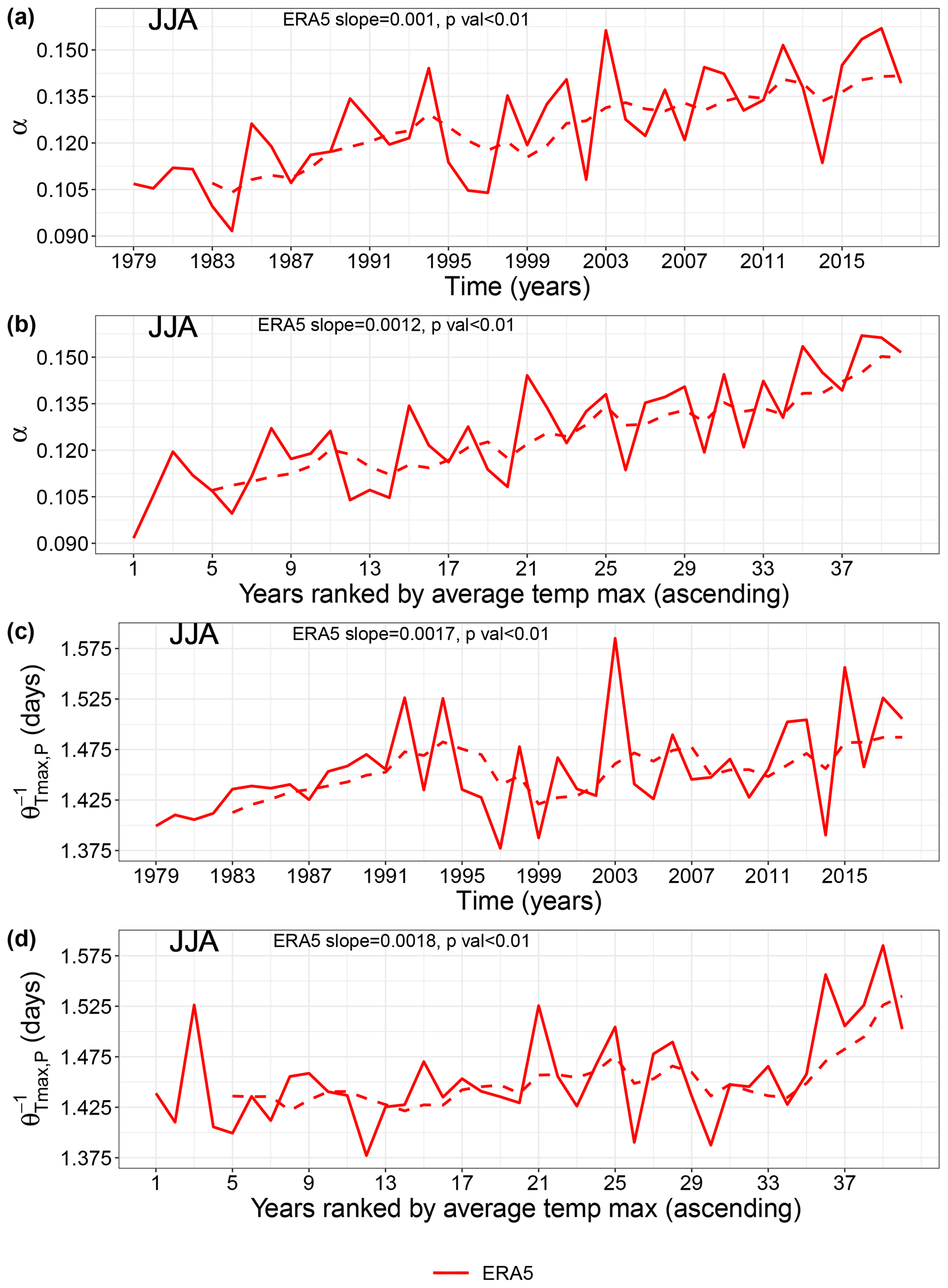
Figure 1Co-recurrence ratio (α) and local co-persistence JJA means for ERA5 during the 1979–2018 period over the Mediterranean (MED). (a) α JJA yearly means; (b) α ranked according to ascending JJA average Tmax; (c) JJA yearly means; and (d) ranked according to ascending JJA average Tmax. The dashed lines are 5-year centred moving averages. The Sen's slopes and p values are also shown.
We next compute the local co-persistence () trends during JJA (Figs. 1c and S1c) in analogy to Figs. 1a and S1a. The significant upward trends (p value < 0.01 for ERA5 and ERA-Interim and p value < 0.05 for ERA5 ensemble) in imply a trend towards longer-lasting joint spatial patterns of Tmax and P over the MED within the observational period. By computing the co-persistence trends with only warm–dry days, similar results are obtained (not shown), pointing towards increasingly long warm–dry events over the region. As for α, changes in co-persistence map directly onto changes in average Tmax in JJA (Figs. 1d and S1d). Interestingly, there is a clear peak in during summer 2003 for all reanalysis products, coinciding with the extreme 2003 European heatwave (Black et al., 2004; Fischer et al., 2007; Stott et al., 2004). Moreover, similar trends as for Fig. 1 are obtained when computing α and for land-only grid points (Fig. S5a–d). The same, albeit with lower values, applies for α trends over sea only (Fig. S5e and f), while in this case does not show statistical significance (Fig. S5g and h). The latter may be related to the damping role of the sea on air temperatures, although a more systematic analysis would be required to ascertain this. The trends in reflect trends in the (univariate) local persistence of Tmax () and P () (Figs. 2 and S6). They also at least in part explain the trends in α, since one may intuitively expect a higher co-persistence to lead to a higher co-recurrence ratio. We do indeed find that and α are positively and significantly correlated in JJA (not shown). Trends in (Figs. 2a and S6a) are stronger than those in (Figs. 2b and S6b). This strengthens our interpretation of Tmax as playing a predominant role in setting the observed positive trends in the dynamical metrics.
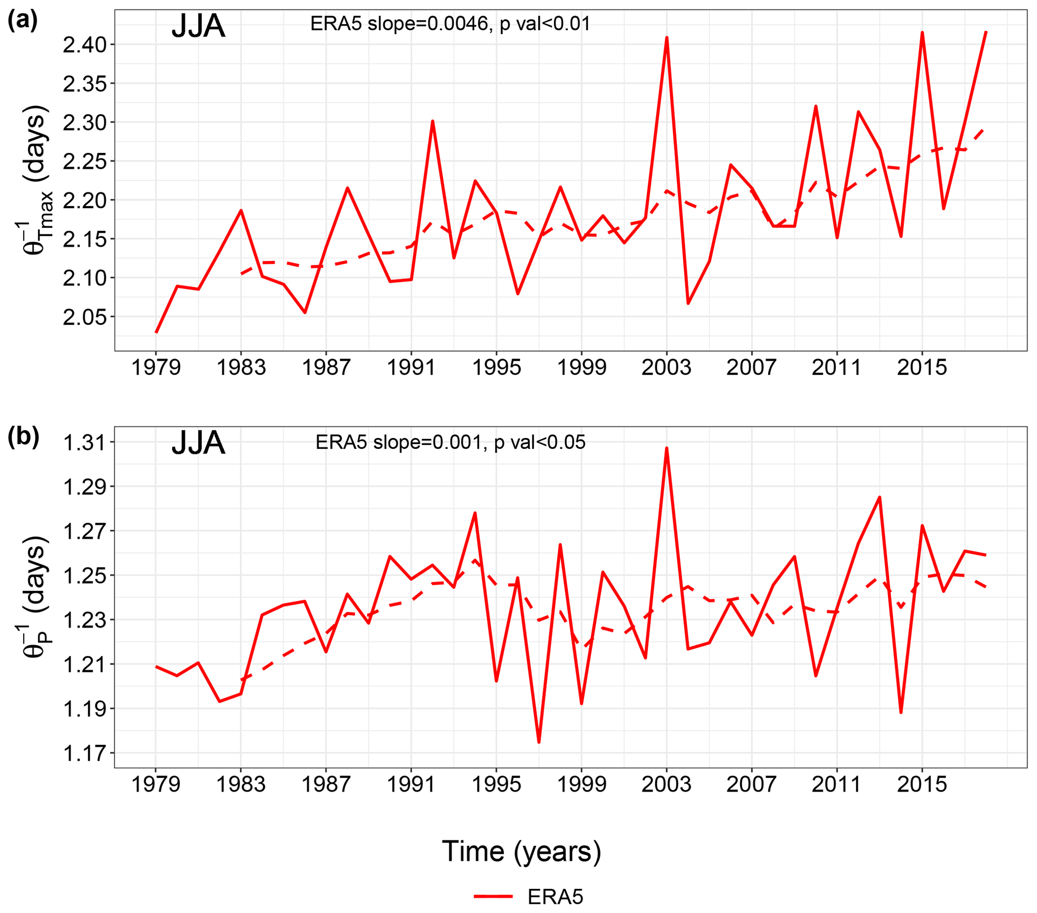
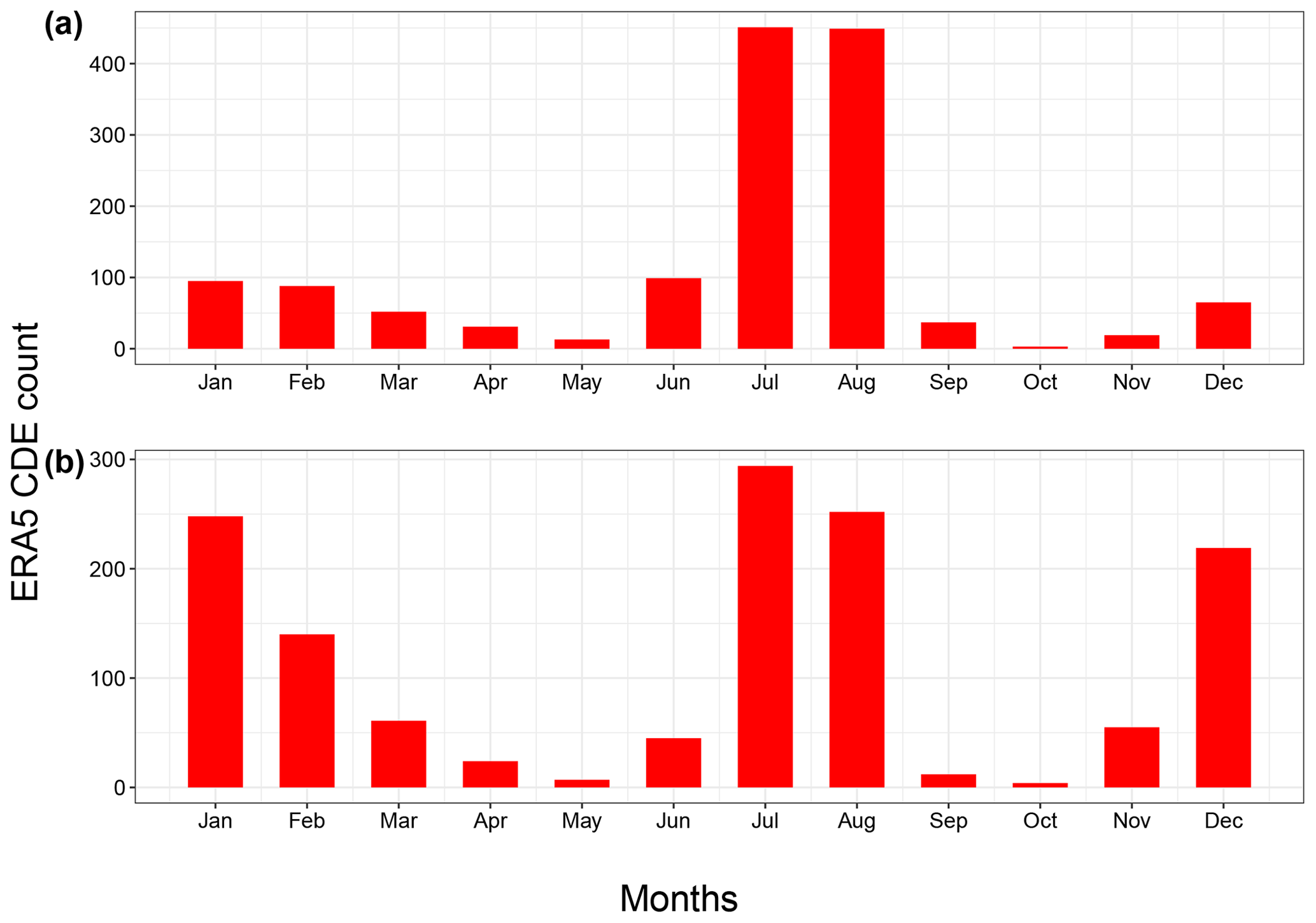
Figure 3Monthly counts of compound dynamical extremes (CDEs) for ERA5 during 1979–2018 over the MED. (a) α computed from Tmax and P; (b) α computed from Tmin and P. CDEs are defined as α daily observations >90th quantile of the α distribution for the full dataset.

Figure 4JJA and DJF anomaly means of (a, b) SLP, (c, d) Tmax and Tmin, and (e, f) P during CDE days. The data are from the ERA5 reanalysis during 1979–2018. α for JJA is computed from Tmax and P, whereas that for DJF is computed from Tmin and P. Stippling shows statistically significant anomalies (p value < 0.05, Mann–Whitney one-tailed test). The Bonferroni correction is applied to all p values.
4.1 Seasonality of CDEs
We next investigate the temporal distribution of CDEs. For α computed on Tmax and P, all three reanalysis products display most of the CDEs clustering in July and August, with a secondary peak in DJF (Figs. 3a and S7a). For α computed on Tmin and P, most CDEs occur during DJF, July and August (Figs. 3b and S7b). This holds for all three reanalysis products. The large number of CDEs during July and August (Figs. 3b and S7b) reflect compound warm–dry events (not shown). We further note that, notwithstanding the previously mentioned correlation between co-persistence and α, the seasonality of extremes – defined analogously to the CDEs – does not reflect that of the CDEs (not shown). For both variable combinations (i.e. Tmax–P and Tmin–P), the two shoulder seasons (i.e. spring and autumn) display very few CDEs. In Faranda et al. (2017a), the authors hypothesized that during autumn and spring the atmospheric flow sits on a saddle-like point of the dynamics, while winter and summer represent more stable basins of attraction. Assuming that distinct attractors does indeed exist for winter and summer, we thus interpret these low CDE counts as the result of the atmospheric flow exploring both summer and winter configurations, resulting in rarer co-recurrences.
4.2 Pressure, temperature and precipitation anomalies during CDEs
During JJA, CDEs correspond to statistically significant positive SLP anomalies over the Western MED (north-western Africa) and the Anatolia–Black Sea region. These are separated by negative SLP anomalies spanning the Aegean Sea, the Levant and northern Egypt (Figs. 4a and S8a and b). These SLP anomalies are in turn associated with significant warm Tmax anomalies over most of the MED, with a particularly warm Balkan Peninsula, and a negative anomaly over central northern Africa, to the east of the positive SLP anomaly (Figs. 4c and S8c and d). Lastly, we observe weak dry P anomalies over the Black Sea (Figs. 4e and S8e and f) and stronger wet P anomalies over the Alps. The latter correspond to statistically significant convective available potential energy (CAPE, J kg−1) positive anomalies (Fig. S9) and may therefore be linked to localized convective P events. We conclude that JJA CDEs are closely linked to widespread warm Tmax anomalies but have a weaker footprint on P anomalies, except over the Alps.

Figure 5Histograms and cumulative distribution functions (CDFs) of anomaly means of (a) Tmax and (b) P during JJA CDEs and (c) Tmin and (d) P during DJF CDEs. The data are the same as in Fig. 4c–f. The distributions are statistically different from those of all other JJA and DJF days respectively (p value ≪ 0.01, Mann–Whitney one-tailed test).
In DJF we observe an east–west dipole in SLP over the MED, that favours cold-air advection from northern Europe to the Balkans, parts of the Italian Peninsula and the southern and Eastern MED (Figs.4b and S10a and b). Indeed, negative and significant Tmin anomalies are observed over most of the MED region (Figs. 4d and S10c and d). The Eastern MED also displays significant positive P anomalies (Figs. 4f and S10e and f). The statistically significant (p value < 0.05) negative SLP anomalies over the Eastern MED are reminiscent of the footprint of Cyprus Lows, which are the main rain-bearing systems over the region (Alpert et al., 2004; Saaroni et al., 2010) (Figs. 4b and S10a and b). Cyprus Lows are also associated with the majority of wintertime cold spells over the Eastern MED (Hochman et al., 2020), and we do indeed find that some of the P anomalies over the Eastern MED are snowfall events, particularly over the Balkans, Turkey and Lebanon (Fig. S11). We thus conclude that CDEs are associated with wintertime cold–wet compound events over the Eastern MED.
As a proxy for the variability within our composites in Fig. 4, we compute the standard deviations (SDs) of the anomalies (not shown). We observe that SLP SDs are larger over the northern and central MED, while temperature SDs are larger over land compared to the sea – the latter a natural consequence of the sea's large thermal inertia. Finally, precipitation SDs are larger where the higher anomaly mean values are reported (i.e. the Alps in JJA and south-eastern MED in DJF), which may be linked to the prevailingly dry summertime conditions in the MED which yield low SDs where little or no rain falls. Similar results are obtained when computing Fig. 4 using only extreme anomalies (anom > 90th and anom < 10th quantiles) matching CDEs, although the JJA positive SLP anomalies are less geographically extensive (Fig. S12).
4.3 Distributions of temperature and precipitation anomaly means
We next test empirically whether the CDEs highlighted above have a systematic link to compound JJA warm–dry and DJF cold–wet events. During JJA, Tmax and P daily anomaly means, computed for each grid point during CDEs, are predominantly warm (85 %) and dry (79 %) respectively (Fig.5a and b). Similar results are also obtained for ERA-Interim and the ERA5 ensemble (Fig. S13). P anomalies tend to cluster around zero, owing to the overall dry summertime climate of the region, although as noted above they do show a preference for negative (dry) values (Figs. 5b and S13b and d). A Mann–Whitney one-tailed test between the anomaly means during CDEs versus all other days in JJA results in statistically significant differences (p value ≪ 0.01) for all reanalysis products for both Tmax and P. This implies that CDEs are significantly warmer and drier than other JJA days.
In DJF, most of the Tmin and P anomaly means are cold (78 %) and wet (58 %) respectively for ERA5 (Fig. 5c and d) and the other reanalysis products (Fig. S14). Again, a Mann–Whitney one-tailed test between anomaly means during CDEs and all other DJF days highlights statistically significant (p value ≪ 0.01) differences for all reanalysis products, except ERA-Interim's P (p value < 0.05). This implies that CDEs are significantly colder and wetter than all other DJF days. The CDEs therefore present a somewhat mirror image of the preferred anomalies seen in the geographical anomaly composites for both JJA and DJF.
4.4 Spatial patterns of compound warm–dry and cold–wet events
We next complement the statistical information provided by the histograms and CDFs with spatial distributions of percentage (%) match between CDEs and compound events. Put simply, for each grid point in Fig. 6 we identify the days reporting compound events and CDEs and then divide the total number of these days by the total number of CDEs and multiply the resulting number by 100 to obtain the percentage agreement value. Across the MED, a high fraction of CDEs coincide with compound warm–dry events during JJA. Values locally exceed 70 %, meaning that >70 % of all JJA CDEs occur during compound warm–dry events (Figs. 6a and S15). The highest percentages occur in southern Spain, the Balearic Islands, Italy and the Balkans. During DJF, the percentage match between CDEs and compound cold–wet events is lower than that seen for warm–dry JJA events (<50 %) (Figs. 6b and S16). The highest percentage occurs over the Eastern MED sea, between the coastlines of Libya, Egypt, Greece and Turkey. In both JJA and DJF the vast majority of observations (%) are statistically significant at the 1 % level (p value < 0.01; Figs. 6 and S15 and S16).
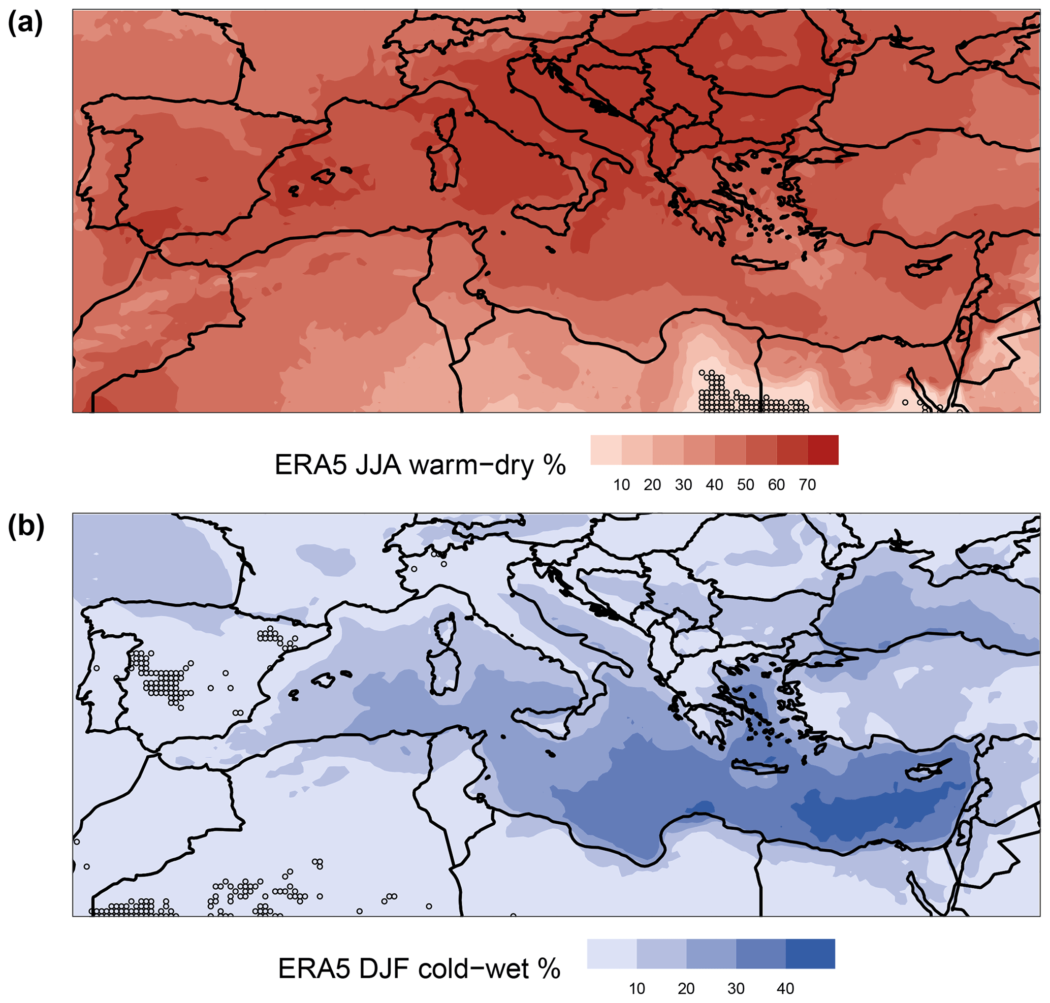
Figure 6Percentage (%) of CDEs occurring during compound (a) JJA warm–dry and (b) DJF cold–wet events. The data are from the ERA5 reanalysis during 1979–2018. Stippling represent values not statistically significant at the 1 % level (p value ≥ 0.01).
In this paper, we analysed compound warm–dry (cold–wet) events during JJA (DJF) over the Mediterranean (MED) through the lens of dynamical systems theory. We specifically computed a measure of coupling (α) between daily maximum temperature (Tmax) and total precipitation (P) during JJA and daily minimum temperature (Tmin) and P during DJF. We then identified days when the two variables are strongly coupled (α>90th percentile of its full distribution) and termed them CDEs. We further computed a dynamical systems measure of the persistence of large-scale configurations in the above variables (θ−1), considering them both individually and in pairs. We made use of the ERA5 dataset but also replicated the analyses with ERA-Interim and the ERA5 10-member ensemble (see Supplement). We generally found good agreement between the different reanalysis products.
During JJA, both α and display significant upward trends. An upward persistence trend is also found if we focus specifically on warm–dry days. We propose that these trends are driven by surface warming over the MED. A possible physical process driving increasing coupling with increasing temperature is soil drying. Although we did not investigate this in detail here, we found that a decrease in average P is also linked with an upward and significant trend in α (Fig. S17) and that the correlation between Figs. 1b and S17 α values is positive and significant (ρ=0.56, p value < 0.01). Specifically, the increasingly warm summer temperatures and lack of P may lead to significantly lower soil-moisture content, triggering a feedback mechanism that favours persistent warm–dry conditions. However, at this stage, is difficult to discriminate between the prevailing role between Tmax and P in driving the α trends, since they may have a compound or univariate effect. We will therefore keep this investigation for a further work. Consistently with the α trends, we found that CDEs computed from Tmax and P cluster during July and August, whereas CDEs computed from Tmin and P cluster during July, August and DJF. During CDE days, synoptic patterns in JJA show significant positive SLP and warm Tmax anomalies over large parts of the MED and dry but mainly not-significant anomalies for P. The latter is somewhat unsurprising, as the low climatological summertime precipitation over the region effectively prevents the occurrence of large negative precipitation anomalies. Moreover, Tmax anomalies result higher over land than over the sea because the latter's thermal inertia likely plays a damping role during the occurrence of heatwaves. Lastly, the JJA SLP patterns do not point to any clear and documented synoptic structure. It may therefore be possible that CDEs capture several different sets of weather circulation regimes. In DJF, CDEs are associated with significant negative SLP anomalies and cold–wet anomalies centred over the Eastern MED. The distributions of anomalies occurring during CDEs are significantly different (p values of <0.01 or <0.05) from the ones recorded during all other days. Lastly, we found that CDEs correspond to a heightened frequency of positive Tmax and negative P anomalies during JJA and to a heightened frequency of negative Tmin and positive P anomalies during DJF over large parts of the MED. The percentages of CDEs matching cold–wet days during DJF are, however, lower than those found during summer for warm–dry days.
The findings that summertime Tmax and P have become more strongly coupled over the last 40 years and that the persistence of warm–dry days has increased are in agreement with Zscheischler and Seneviratne (2017) and Manning et al. (2019). The former study showed that land–atmosphere feedbacks in a warmer world may lead to an increase in warm–dry summers larger than what may be expected by analysing the projected temperature and precipitation changes as single variables. However, the work of Zscheischler and Seneviratne (2017) differs from ours since they made use of detrended temperature and precipitation datasets. Whereas Manning et al. (2019) found that rising temperatures drive an increased probability of dry and hot events in Europe, with dry periods becoming hotter and hence pointing to a significant thermodynamic response of compound events due to global warming. Assuming a continued increase in future temperatures, we may therefore expect ongoing positive JJA α and trends, leading to a higher frequency of compound JJA warm–dry events.
The analysis of DJF CDEs, matching cold–wet events, points to very different dynamics. Here, the largest anomalies in SLP, Tmin and P are found over the Eastern MED and are reminiscent of the footprint of Cyprus Lows. These are wintertime synoptic systems that play a predominant role in driving concurrent cold spells and heavy precipitation events over the Levant (e.g. Hochman et al., 2019). Our findings show no significant increase in α values during DJF, in line with studies suggesting a decrease in Cyprus Low frequency, persistence and associated precipitation over the Eastern MED (Hochman et al., 2020, 2018; Peleg et al., 2015).
Our findings highlight a close connection between CDEs, computed from dynamical systems coupling and compound JJA warm–dry and DJF cold–wet events over the MED. The link between CDEs and compound events likely issues from the fact that, in both cases, the data reflect anomalous (or highly coupled) conditions for the atmospheric variables being studied. It is of particular interest that α distinguishes between JJA warm–dry and DJF cold–wet compound events. However, results obtained from our dynamical systems approach may be sensitive to the size and location of the geographical domain(s) under study. For such a reason, it is important to constrain the dynamical systems analysis only over a geographical area justified by, for example, physical process understanding or impact assessment. In the latter case, one may be interested to calculate compound climate risks by making use of CDEs as a measure of the multi-hazard component or to link α with (long enough) impact datasets, such as insurance losses, crop yield or renewable energy production.
Based on our results, we learn the following: (i) the coupling between temperature and precipitation at large scales is driven by specific regions and processes (e.g. Cyprus Low), and therefore it does not always reflect the whole MED; (ii) the coupling results are sensitive even to non-extreme events, and thus the co-recurrence ratio (α) may be fruitfully used in forthcoming studies to elucidate potential future seasonal climatic changes over the MED; and (iii) our results provide information on specific factors that are driving the changes in α (e.g. surface warming). In the future, we envisage making use of global CMIP6 data under different shared socio-economic pathways (SSPs) up to 2100 (O'Neill et al., 2016) and abrupt climate change simulations (e.g. 4×CO2) (Eyring et al., 2016). These investigations may also shed some light on possible tipping points over the MED (Lenton et al., 2008; Lenton, 2011).
The ERA5, ERA5 10-member ensemble and ERA-Interim reanalysis datasets used in this work are freely available from the European Centre for Medium-Range Weather Forecasts (ECMWF) websites https://cds.climate.copernicus.eu/ (last access: 28 August 2020) (C3S, 2017) and https://apps.ecmwf.int/datasets/data/interim-full-daily/levtype=sfc/ (last access: 28 August 2020) (Dee et al., 2011).
The supplement related to this article is available online at: https://doi.org/10.5194/esd-11-793-2020-supplement.
PDL designed the study, performed the analyses and created the figures. GM, DF and DC contributed to the methods and study design. PDL and GM wrote the first paper draft. All the authors contributed to the writing.
The authors declare that they have no conflicts of interest.
This article is part of the special issue “Understanding compound weather and climate events and related impacts (BG/ESD/HESS/NHESS inter-journal SI)”. It is not associated with a conference.
The data analysis was performed on the VU HPC BAZIS cluster. The authors would like to thank the three referees and the editor for their constructive comments, which significantly improved the paper.
This is TiPES contribution no. 15. This project has received funding from the European Union's Horizon 2020 research and innovation programme under grant agreement no. 820970. Paolo De Luca was also supported by an E-COST STSM (DAMOCLES, Action CA17109). Gabriele Messori was partly supported by the Swedish Research Council Vetenskapsrådet under grant agreement no. 2016-03724. Philip J. Ward was supported by a VIDI grant from the Dutch Research Council (NWO, grant no.: 016.161.324).
This paper was edited by Jakob Zscheischler and reviewed by Olivia Romppainen-Martius, Vera Melinda Galfi, and Emanuele Bevacqua.
Abadi, M., Freitas, A. C. M., and Freitas, J. M.: Dynamical counterexamples regarding the Extremal Index and the mean of the limiting cluster size distribution, arXiv preprint: arXiv:180802970, 2018. a
Alpert, P., Osetinsky, I., Ziv, B., and Shafir, H.: Semi-objective classification for daily synoptic systems: application to the eastern Mediterranean climate change, Int. J. Climatol., 24, 1001–1011, https://doi.org/10.1002/joc.1036, 2004. a
Barcikowska, M. J., Kapnick, S. B., Krishnamurty, L., Russo, S., Cherchi, A., and Folland, C. K.: Changes in the future summer Mediterranean climate: contribution of teleconnections and local factors, Earth Syst. Dynam., 11, 161–181, https://doi.org/10.5194/esd-11-161-2020, 2020. a
Barriopedro, D., Fischer, E. M., Luterbacher, J., Trigo, R. M., and García-Herrera, R.: The Hot Summer of 2010: Redrawing the Temperature Record Map of Europe, Science, 332, 220–224, https://doi.org/10.1126/science.1201224, 2011. a
Beniston, M., Stephenson, D. B., Christensen, O. B., Ferro, C. A. T., Frei, C., Goyette, S., Halsnaes, K., Holt, T., Jylhä, K., Koffi, B., Palutikof, J., Schöll, R., Semmler, T., and Woth, K.: Future extreme events in European climate: an exploration of regional climate model projections, Climatic Change, 81, 71–95, https://doi.org/10.1007/s10584-006-9226-z, 2007. a, b
Bisci, C., Fazzini, M., Beltrando, G., Cardillo, A., and Romeo, V.: The February 2012 exceptional snowfall along the Adriatic side of Central Italy, Meteorol. Z., 21, 503–508, https://doi.org/10.1127/0941-2948/2012/0536, 2012. a
Black, E., Blackburn, M., Harrison, G., Hoskins, B., and Methven, J.: Factors contributing to the summer 2003 European heatwave, Weather, 59, 217–223, https://doi.org/10.1256/wea.74.04, 2004. a
Bonferroni, C.: Teoria statistica delle classi e calcolo delle probabilita, Pubblicazioni del R Istituto Superiore di Scienze Economiche e Commericiali di Firenze, 8, 3–62, 1936. a
Bosch, X.: European heatwave causes misery and deaths, Lancet, 362, 543, https://doi.org/10.1016/S0140-6736(03)14155-4, 2003. a
Cherchi, A., Annamalai, H., Masina, S., Navarra, A., and Alessandri, A.: Twenty-first century projected summer mean climate in the Mediterranean interpreted through the monsoon-desert mechanism, Clim. Dynam., 47, 2361–2371, https://doi.org/10.1007/s00382-015-2968-4, 2016. a
Corder, G. W. and Foreman, D. I.: Nonparametric Statistics: A Step-by-Step Approach, Wiley, Hoboken, New Jersey, 2014. a
Couasnon, A., Eilander, D., Muis, S., Veldkamp, T. I. E., Haigh, I. D., Wahl, T., Winsemius, H. C., and Ward, P. J.: Measuring compound flood potential from river discharge and storm surge extremes at the global scale, Nat. Hazards Earth Syst. Sci., 20, 489–504, https://doi.org/10.5194/nhess-20-489-2020, 2020. a
C3S – Copernicus Climate Change Service: ERA5: Fifth generation of ECMWF atmospheric reanalyses of the global climate, CDS – Copernicus Climate Change Service Climate Data Store, available at: https://cds.climate.copernicus.eu/cdsapp#!/home (last access: 28 August 2020), 2017. a, b, c
Dee, D. P., Uppala, S. M., Simmons, A. J., Berrisford, P., Poli, P., Kobayashi, S., Andrae, U., Balmaseda, M. A., Balsamo, G., Bauer, P., Bechtold, P., Beljaars, A. C. M., van de Berg, L., Bidlot, J., Bormann, N., Delsol, C., Dragani, R., Fuentes, M., Geer, A. J., Haimberger, L., Healy, S. B., Hersbach, H., Hólm, E. V., Isaksen, L., Kållberg, P., Köhler, M., Matricardi, M., McNally, A. P., Monge-Sanz, B. M., Morcrette, J.-J., Park, B.-K., Peubey, C., de Rosnay, P., Tavolato, C., Thépaut, J.-N., and Vitart, F.: The ERA-Interim reanalysis: configuration and performance of the data assimilation system, Q. J. Roy. Meteorol. Soc., 137, 553–597, https://doi.org/10.1002/qj.828, 2011. a, b
De Luca, P., Hillier, J., Wilby, R., Quinn, N., and Harrigan, S.: Extreme multi-basin flooding linked with extra-tropical cyclones, Environ. Res. Lett., 12, 114009, https://doi.org/10.1088/1748-9326/aa868e, 2017. a
De Luca, P., Messori, G., Pons, F., and Faranda, D.: Dynamical Systems Theory Sheds New Light on Compound Climate Extremes in Europe and Eastern North America, Q. J. Roy. Meteorol. Soc., 146, 1636–1650, https://doi.org/10.1002/qj.3757, 2020a. a, b
De Luca, P., Messori, G., Wilby, R. L., Mazzoleni, M., and Di Baldassarre, G.: Concurrent wet and dry hydrological extremes at the global scale, Earth Syst. Dynam., 11, 251–266, https://doi.org/10.5194/esd-11-251-2020, 2020b. a
de Ruiter, M. C., Couasnon, A., van den Homberg, M. J. C., Daniell, J. E., Gill, J. C., and Ward, P. J.: Why We Can No Longer Ignore Consecutive Disasters, Earth's Future, 8, e2019EF001425, https://doi.org/10.1029/2019EF001425, 2020. a, b
Eyring, V., Bony, S., Meehl, G. A., Senior, C. A., Stevens, B., Stouffer, R. J., and Taylor, K. E.: Overview of the Coupled Model Intercomparison Project Phase 6 (CMIP6) experimental design and organization, Geosci. Model Dev., 9, 1937–1958, https://doi.org/10.5194/gmd-9-1937-2016, 2016. a
Faranda, D.: An attempt to explain recent trends in European snowfall extremes, Weather Clim. Dynam. Discuss., 2019, 1–20, https://doi.org/10.5194/wcd-2019-15, 2019. a
Faranda, D., Lucarini, V., Turchetti, G., and Vaienti, S.: Numerical Convergence of the Block-Maxima Approach to the Generalized Extreme Value Distribution, J. Stat. Phys., 145, 1156–1180, https://doi.org/10.1007/s10955-011-0234-7, 2011. a
Faranda, D., Messori, G., Alvarez-Castro, M. C., and Yiou, P.: Dynamical properties and extremes of Northern Hemisphere climate fields over the past 60 years, Nonlin. Processes Geophys., 24, 713–725, https://doi.org/10.5194/npg-24-713-2017, 2017a. a, b
Faranda, D., Messori, G., and Yiou, P.: Dynamical proxies of North Atlantic predictability and extremes, Scient. Rep., 7, 41278, https://doi.org/10.1038/srep41278, 2017b. a, b, c, d
Faranda, D., Alvarez-Castro, M. C., Messori, G., Rodrigues, D., and Yiou, P.: The hammam effect or how a warm ocean enhances large scale atmospheric predictability, Nat. Commun., 10, 1–7, https://doi.org/10.1038/s41467-019-09305-8, 2019. a, b, c, d
Faranda, D., Messori, G., and Yiou, P.: Diagnosing concurrent drivers of weather extremes: application to warm and cold days in North America, Clim. Dynam., 54, 2187–2201, https://doi.org/10.1007/s00382-019-05106-3, 2020. a, b, c, d, e
Fischer, E. M. and Schär, C.: Consistent geographical patterns of changes in high-impact European heatwaves, Nat. Geosci., 3, 398–403, https://doi.org/10.1038/ngeo866, 2010. a
Fischer, E. M., Seneviratne, S. I., Vidale, P. L., Lüthi, D., and Schär, C.: Soil Moisture–Atmosphere Interactions during the 2003 European Summer Heat Wave, J. Climate, 20, 5081–5099, https://doi.org/10.1175/JCLI4288.1, 2007. a
Freitas, A. C. M., Freitas, J. M., and Todd, M.: Hitting time statistics and extreme value theory, Probabil. Theor. Relat. Fields, 147, 675–710, https://doi.org/10.1007/s00440-009-0221-y, 2010. a, b, c
Giannakopoulos, C., Sager, P. L., Bindi, M., Moriondo, M., Kostopoulou, E., and Goodess, C.: Climatic changes and associated impacts in the Mediterranean resulting from a 2 ∘C global warming, Global Planet. Change, 68, 209–224, https://doi.org/10.1016/j.gloplacha.2009.06.001, 2009. a, b, c
Giorgi, F.: Climate change hot-spots, Geophys. Res. Lett., 33, L08707, https://doi.org/10.1029/2006GL025734, 2006. a
Giorgi, F. and Lionello, P.: Climate change projections for the Mediterranean region, Global Planet. Change, 63, 90–104, https://doi.org/10.1016/j.gloplacha.2007.09.005, 2008. a, b, c
Goubanova, K. and Li, L.: Extremes in temperature and precipitation around the Mediterranean basin in an ensemble of future climate scenario simulations, Global Planet. Change, 57, 27–42, https://doi.org/10.1016/j.gloplacha.2006.11.012, 2007. a, b
Hochman, A., Harpaz, T., Saaroni, H., and Alpert, P.: The seasons' length in 21st century CMIP5 projections over the eastern Mediterranean, Int. J. Climatol., 38, 2627–2637, https://doi.org/10.1002/joc.5448, 2018. a, b
Hochman, A., Alpert, P., Harpaz, T., Saaroni, H., and Messori, G.: A new dynamical systems perspective on atmospheric predictability: Eastern Mediterranean weather regimes as a case study, Sci. Adv., 5, eaau0936, https://doi.org/10.1126/sciadv.aau0936, 2019. a, b, c, d
Hochman, A., Alpert, P., Kunin, P., Rostkier-Edelstein, D., Harpaz, T., Saaroni, H., and Messori, G.: The dynamics of cyclones in the twentyfirst century: the Eastern Mediterranean as an example, Clim. Dynam., 54, 561–574, https://doi.org/10.1007/s00382-019-05017-3, 2020. a, b, c, d
Hoerling, M., Eischeid, J., Perlwitz, J., Quan, X., Zhang, T., and Pegion, P.: On the Increased Frequency of Mediterranean Drought, J. Climate, 25, 2146–2161, https://doi.org/10.1175/JCLI-D-11-00296.1, 2012. a, b
Hu, Y. and Fu, Q.: Observed poleward expansion of the Hadley circulation since 1979, Atmos. Chem. Phys., 7, 5229–5236, https://doi.org/10.5194/acp-7-5229-2007, 2007. a
Kim, G.-U., Seo, K.-H., and Chen, D.: Climate change over the Mediterranean and current destruction of marine ecosystem, Scient. Rep., 9, 18813, https://doi.org/10.1038/s41598-019-55303-7, 2019. a
Lenton, T. M.: Early warning of climate tipping points, Nat. Clim. Change, 1, 201–209, https://doi.org/10.1038/nclimate1143, 2011. a
Lenton, T. M., Held, H., Kriegler, E., Hall, J. W., Lucht, W., Rahmstorf, S., and Schellnhuber, H. J.: Tipping elements in the Earth's climate system, P. Natl. Acad. Sci. USA, 105, 1786–1793, https://doi.org/10.1073/pnas.0705414105, 2008. a
Li, Y., Ye, W., Wang, M., and Yan, X.: Climate change and drought: a risk assessment of crop-yield impacts, Clim. Res., 39, 31–46, https://doi.org/10.3354/cr00797, 2009. a
Lucarini, V., Faranda, D., and Wouters, J.: Universal Behaviour of Extreme Value Statistics for Selected Observables of Dynamical Systems, J. Stat. Phys., 147, 63–73, https://doi.org/10.1007/s10955-012-0468-z, 2012. a, b, c
Mann, H. B.: Nonparametric Tests Against Trend, Econometrica, 13, 245–259, 1945. a
Mann, H. B. and Whitney, D. R.: On a test of whether one of two random variables is stochastically larger than the other, Ann. Math. Stat., 18, 50–60, 1947. a
Manning, C., Widmann, M., Bevacqua, E., Loon, A. F. V., Maraun, D., and Vrac, M.: Increased probability of compound long-duration dry and hot events in Europe during summer (1950–2013), Environ. Res. Lett., 14, 094006, https://doi.org/10.1088/1748-9326/ab23bf, 2019. a, b, c
Mariotti, A.: Recent Changes in the Mediterranean Water Cycle: A Pathway toward Long-Term Regional Hydroclimatic Change?, J. Climate, 23, 1513–1525, https://doi.org/10.1175/2009JCLI3251.1, 2010. a
Mariotti, A., Pan, Y., Zeng, N., and Alessandri, A.: Long-term climate change in the Mediterranean region in the midst of decadal variability, Clim. Dynam., 44, 1437–1456, https://doi.org/10.1007/s00382-015-2487-3, 2015. a
Messori, G., Caballero, R., and Faranda, D.: A dynamical systems approach to studying midlatitude weather extremes, Geophys. Res. Lett., 44, 3346–3354, https://doi.org/10.1002/2017GL072879, 2017. a, b
Moftakhari, H. R., AghaKouchak, A., Sanders, B. F., and Matthew, R. A.: Cumulative hazard: The case of nuisance flooding, Earth's Future, 5, 214–223, https://doi.org/10.1002/2016EF000494, 2017. a
Moloney, N. R., Faranda, D., and Sato, Y.: An overview of the extremal index, Chaos, 29, 022101, https://doi.org/10.1063/1.5079656, 2019. a
Nykjaer, L.: Mediterranean Sea surface warming 1985–2006, Clim. Res., 39, 11–17, https://doi.org/10.3354/cr00794, 2009. a
O'Neill, B. C., Tebaldi, C., van Vuuren, D. P., Eyring, V., Friedlingstein, P., Hurtt, G., Knutti, R., Kriegler, E., Lamarque, J.-F., Lowe, J., Meehl, G. A., Moss, R., Riahi, K., and Sanderson, B. M.: The Scenario Model Intercomparison Project (ScenarioMIP) for CMIP6, Geosci. Model Dev., 9, 3461–3482, https://doi.org/10.5194/gmd-9-3461-2016, 2016. a
Peleg, N., Bartov, M., and Morin, E.: CMIP5-predicted climate shifts over the East Mediterranean: implications for the transition region between Mediterranean and semi-arid climates, Int. J. Climatol., 35, 2144–2153, https://doi.org/10.1002/joc.4114, 2015. a, b
Rodrigues, D., Alvarez-Castro, M. C., Messori, G., Yiou, P., Robin, Y., and Faranda, D.: Dynamical Properties of the North Atlantic Atmospheric Circulation in the Past 150 Years in CMIP5 Models and the 20CRv2c Reanalysis, J. Climate, 31, 6097–6111, https://doi.org/10.1175/JCLI-D-17-0176.1, 2018. a
Rodwell, M. J. and Hoskins, B. J.: Monsoons and the dynamics of deserts, Q. J. Roy. Meteorol. Soc., 122, 1385–1404, https://doi.org/10.1002/qj.49712253408, 1996. a
Saaroni, H., Halfon, N., Ziv, B., Alpert, P., and Kutiel, H.: Links between the rainfall regime in Israel and location and intensity of Cyprus lows, Int. J. Climatol., 30, 1014–1025, https://doi.org/10.1002/joc.1912, 2010. a
Samuels, R., Hochman, A., Baharad, A., Givati, A., Levi, Y., Yosef, Y., Saaroni, H., Ziv, B., Harpaz, T., and Alpert, P.: Evaluation and projection of extreme precipitation indices in the Eastern Mediterranean based on CMIP5 multi-model ensemble, Int. J. Climatol., 38, 2280–2297, https://doi.org/10.1002/joc.5334, 2018. a, b
Scher, S. and Messori, G.: Predicting weather forecast uncertainty with machine learning, Q. J. Roy. Meteorol. Soc., 144, 2830–2841, https://doi.org/10.1002/qj.3410, 2018. a
Scoccimarro, E., Gualdi, S., Bellucci, A., Zampieri, M., and Navarra, A.: Heavy precipitation events over the Euro-Mediterranean region in a warmer climate: results from CMIP5 models, Reg. Environ. Change, 16, 595–602, https://doi.org/10.1007/s10113-014-0712-y, 2016. a, b
Seager, R., Liu, H., Henderson, N., Simpson, I., Kelley, C., Shaw, T., Kushnir, Y., and Ting, M.: Causes of Increasing Aridification of the Mediterranean Region in Response to Rising Greenhouse Gases, J. Climate, 27, 4655–4676, https://doi.org/10.1175/JCLI-D-13-00446.1, 2014. a
Seeherman, J. and Liu, Y.: Effects of extraordinary snowfall on traffic safety, Accident Anal. Prevent., 81, 194–203, https://doi.org/10.1016/j.aap.2015.04.029, 2015. a
Seidel, D. J., Fu, Q., Randel, W. J., and Reichler, T. J.: Widening of the tropical belt in a changing climate, Nat. Geosci., 1, 21–24, https://doi.org/10.1038/ngeo.2007.38, 2008. a
Sen, P. K.: Estimates of the Regression Coefficient Based on Kendall's Tau, J. Am. Stat. Assoc., 63, 1379–1389, https://doi.org/10.1080/01621459.1968.10480934, 1968. a
Shaposhnikov, D., Revich, B., Bellander, T., Bedada, G. B., Bottai, M., Kharkova, T., Kvasha, E., Lezina, E., Lind, T., Semutnikova, E., and Pershagen, G.: Mortality related to air pollution with the moscow heat wave and wildfire of 2010, Epidemiology, 25, 359–364, https://doi.org/10.1097/EDE.0000000000000090, 2014. a
Shohami, D., Dayan, U., and Morin, E.: Warming and drying of the eastern Mediterranean: Additional evidence from trend analysis, J. Geophys. Res.-Atmos., 116, D22101, https://doi.org/10.1029/2011JD016004, 2011. a
Stott, P. A., Stone, D. ., and Allen, M. R.: Human contribution to the European heatwave of 2003, Nature, 432, 610–614, https://doi.org/10.1038/nature03089, 2004. a
Süveges, M.: Likelihood estimation of the extremal index, Extremes, 10, 41–55, https://doi.org/10.1007/s10687-007-0034-2, 2007. a
Totz, S., Petri, S., Lehmann, J., and Coumou, D.: Regional Changes in the Mean Position and Variability of the Tropical Edge, Geophys. Res. Lett., 45, 12076–12084, https://doi.org/10.1029/2018GL079911, 2018. a
Tramblay, Y. and Somot, S.: Future evolution of extreme precipitation in the Mediterranean, Climatic Change, 151, 289–302, https://doi.org/10.1007/s10584-018-2300-5, 2018. a
Wang, B., Liu, J., Kim, H.-J., Webster, P. J., and Yim, S.-Y.: Recent change of the global monsoon precipitation (1979–2008), Clim. Dynam., 39, 1123–1135, https://doi.org/10.1007/s00382-011-1266-z, 2012. a
Ward, P. J., Couasnon, A., Eilander, D., Haigh, I. D., Hendry, A., Muis, S., Veldkamp, T. I. E., Winsemius, H. C., and Wahl, T.: Dependence between high sea-level and high river discharge increases flood hazard in global deltas and estuaries, Environ. Res. Lett., 13, 084012, https://doi.org/10.1088/1748-9326/aad400, 2018. a
Zampieri, M., Ceglar, A., Dentener, F., and Toreti, A.: Wheat yield loss attributable to heat waves, drought and water excess at the global, national and subnational scales, Environ. Res. Lett., 12, 064008, https://doi.org/10.1088/1748-9326/aa723b, 2017. a
Zappa, G., Hawcroft, M. K., Shaffrey, L., Black, E., and Brayshaw, D. J.: Extratropical cyclones and the projected decline of winter Mediterranean precipitation in the CMIP5 models, Clim. Dynam., 45, 1727–1738, https://doi.org/10.1007/s00382-014-2426-8, 2015. a
Zscheischler, J. and Seneviratne, S. I.: Dependence of drivers affects risks associated with compound events, Sci. Adv., 3, e1700263, https://doi.org/10.1126/sciadv.1700263, 2017. a, b
Zscheischler, J., Westra, S., van den Hurk, B., Seneviratne, S., Ward, P., Pitman, A., AghaKouchak, A., Bresch, D., Leonard, M., Wahl, T., and Zhang, X.: Future climate risk from compound events, Nat. Clim. Change, 8, 469–477, https://doi.org/10.1038/s41558-018-0156-3, 2018. a
Zscheischler, J., Martius, O., Westra, S., Bevacqua, E., Raymond, C., Horton, R. M., van den Hurk, B., AghaKouchak, A., Jézéquel, A., Mahecha, M. D., Maraun, D., Ramos, A. M., Ridder, N. N., Thiery, W., and Vignotto, E.: A typology of compound weather and climate events, Nat. Rev. Earth Environ., 1, 333–347, https://doi.org/10.1038/s43017-020-0060-z, 2020. a, b
- Abstract
- Introduction
- Methods and data
- Temperature–precipitation coupling
- Compound dynamical extremes linked to compound warm–dry and cold–wet events
- Discussion and conclusions
- Data availability
- Author contributions
- Competing interests
- Special issue statement
- Acknowledgements
- Financial support
- Review statement
- References
- Supplement