the Creative Commons Attribution 4.0 License.
the Creative Commons Attribution 4.0 License.
 | 19 Jul 2018
Abyssal plain hills and internal wave turbulence
Hans van Haren
A 400 m long array with 201 high-resolution NIOZ temperature sensors was deployed above a north-east equatorial Pacific hilly abyssal plain for 2.5 months. The sensors sampled at a rate of 1 Hz. The lowest sensor was at 7 m above the bottom (m a.b.). The aim was to study internal waves and turbulent overturning away from large-scale ocean topography. Topography consisted of moderately elevated hills (a few hundred metres), providing a mean bottom slope of one-third of that found at the Mid-Atlantic Ridge (on 2 km horizontal scales). In contrast with observations over large-scale topography like guyots, ridges and continental slopes, the present data showed a well-defined near-homogeneous “bottom boundary layer”. However, its thickness varied strongly with time between < 7 and 100 m a.b. with a mean around 65 m a.b. The average thickness exceeded tidal current bottom-frictional heights so that internal wave breaking dominated over bottom friction. Near-bottom fronts also varied in time (and thus space). Occasional coupling was observed between the interior internal wave breaking and the near-bottom overturning, with varying up- and down- phase propagation. In contrast with currents that were dominated by the semidiurnal tide, 200 m shear was dominant at (sub-)inertial frequencies. The shear was so large that it provided a background of marginal stability for the straining high-frequency internal wave field in the interior. Daily averaged turbulence dissipation rate estimates were between 10−10 and 10−9 m2 s−3, increasing with depth, while eddy diffusivities were of the order of 10−4 m2 s−1. This most intense “near-bottom” internal-wave-induced turbulence will affect the resuspension of sediments.


The mechanical kinetic energy brought into the ocean via tides, atmospheric disturbances and the Earth's rotation governs the motions in the density-stratified ocean interior. On the one hand isopycnals are set into oscillating motions as “internal waves”. On the other hand these oscillating motions deform non-linearly and eventually irreversibly lose their energy to turbulent mixing. Breaking internal waves are suggested to be the dominant source of turbulence in the ocean (e.g. Eriksen, 1982; Gregg, 1989; Thorpe, 2018). This turbulence is vital for life in the ocean, as it dominates the diapycnal redistribution of components and suspended materials. It is also important for the resuspension of bottom materials. Large-scale sloping ocean bottoms are important for both the generation (e.g. Bell, 1975; LeBlond and Mysak, 1978; Morozov, 1995) and the breaking of internal waves (e.g. Eriksen, 1982). Not only the topography around ocean basin edges act as a source–sink of internal waves, but also the topography of ridges, mountain ranges and seamounts distributed over the ocean floor (Baines, 2007). Above sufficiently steep slopes exceeding those of the main internal carrier (e.g. tidal) wave containing the largest energy and > 1 km (> the internal wavelength) horizontal-scale topography, turbulent mixing averages 10 000 times molecular diffusion (e.g. Aucan et al., 2006; van Haren and Gostiaux, 2012). This mixing is considered to have a high potential (Cyr and van Haren, 2016) as the back and forth sloshing of the carrier wave ensures a rapid re-stratification down to within a metre from the sea floor. Apparently, mixed waters are transported into the interior along isopycnals or perhaps along isobaths by advective flows. Sloping large-scale topography has received more scientific interest than abyssal “plains” due to the higher turbulence intensity of internal wave breaking. However, abyssal plains occupy a large part of the ocean and the processes that occur there deserve investigation. For example, hills on the bottom form corrugated topography instead of the seemingly flat bottom and contribute to internal wave generation and breaking. These hills are so numerous (Baines, 2007; Morozov, 2018) that it may be questioned whether the abyssal plain and its overlying waters may be called a “quiescent zone”.
This is because occasional “benthic storms” have been reported to disturb the quiescence, even at great depths > 5000 m (Hollister and McCave, 1984). The effects can be significant on sediment reworking and particles remain resuspended long after the “storm” has passed. Such resuspension has obvious effects on deep-sea benthic biology and remineralization (e.g. Lochte, 1992).
In order to avoid semantic problems, the term “benthic boundary layer” is reserved here for the sediment–water interface (at the bottom of the water phase of the ocean), following common practice by sedimentologists and marine chemists (e.g. Boudreau and Jørgensen, 2001). The term “bottom boundary layer” follows the physical oceanographic convention to describe the lower part of the water phase of the ocean, which is almost uniform in density, using the threshold criterion of the large-scale (100 m) buoyancy frequency N < 3 × 10⁻⁴ s−1. This is the layer of investigation here together with overlying higher density-stratified waters in the interior. The amount of homogeneity is also a subject of study. Historic observations have demonstrated the variability of the abyssal plain bottom boundary layer in space and time (e.g. Wimbush, 1970; Armi and Millard, 1976; Armi and D'Asaro, 1980).
Similar to the ocean interior, waters above abyssal plains are considered calm ocean regions in terms of weak turbulent exchange. However, the (bulk) Reynolds number Re = UL∕ν as a measure for the transition from laminar (“molecular”) to turbulent flow is not small. With the kinematic viscosity m2 s−1 to characterize the molecular water properties, characteristic velocity U ≈ 0.05 m s−1 and length scale L≈30 m of the (internal wave) water flow, Re ≈ 106, which is highly turbulent (e.g. Tennekes and Lumley, 1972; Fritts et al., 2016) even for the unbounded open-ocean and atmosphere interiors.
Both convective instability of the gravitationally unstable denser over less dense water and shear-induced Kelvin–Helmholtz instability KHi are probable for internal wave breaking; for a recent model see Thorpe (2018). Earlier models (e.g. Garrett and Munk, 1972) suggested KHi was dominant over convective instabilities, especially considering the construction of the internal wave field of the smallest vertical scales residing at their lowest frequencies (e.g. LeBlond and Mysak, 1978). Most kinetic energy is found at these frequencies and thus a large background shear is generated (e.g. Alford and Gregg, 2001) through which shorter length-scale waves near the buoyancy frequency propagate, break and overturn. The result is an open-ocean wave field that is highly intermittent, producing a very step-like, non-smooth, sheet-and-layer-structured ocean interior stratification (e.g. Lazier, 1973; Fritts et al., 2016). In the near-surface ocean, such internal wave propagation and deformation “straining” of stratification has been observed to migrate through the density field in space and time.
The lower bound of inertio-gravity wave (IGW) frequencies is determined by the local vertical Coriolis parameter, i.e. the inertial frequency, f=2Ωsinφ, of the Earth rotational vector Ω at latitude φ. This bound becomes significantly modified to lower sub-inertial frequencies under weak stratification (∼ N2) when N < 10f. From non-approximated equations, minimum and maximum IGW frequencies are calculated as [σmin, σmax] = ( using , in which γ is the angle to the north (γ=0 denotes meridional propagation) and the horizontal component of the Coriolis parameter fh=2Ωcosφ becomes important for internal wave dynamics (e.g. LeBlond and Mysak, 1978; Gerkema et al., 2008).
In the present paper, detailed moored observations from a Pacific abyssal plain confirm the Lazier (1973) sheet-and-layer stratification. The new observations are used to investigate the interplay between motions in the stratified interior and the effects on the bottom boundary layer. The small-scale topography may prove non-negligible for internal waves in comparison with large oceanic ridges, seamounts and continental slopes. Following Bell (1975), recent studies demonstrate the potential of substantial internal wave generation by flow over abyssal hills under particular slope and stratification conditions (e.g. Nikurashin et al., 2014; Hibiya et al., 2017). We are interested in the observational details of the IGW-induced turbulent processes.
Observations were made from the German R/V Sonne cruises SO239 and SO240 above the abyssal hills in the Clarion–Clipperton Fracture Zone of the north-east equatorial Pacific Ocean, west of the oriental Pacific Ridge (Fig. 1). The data were collected in the German licence area for polymetallic nodule exploration. The area is not mountainous but also not flat. It is characterized by numerous hills extending several hundred metres above the surrounding sea floor. The average bottom slope is 1.2 ± 0.6∘, computed from Fig. 1b using the 1′ resolution version of the Smith and Sandwell (1997) sea-floor topography. This slope is about 3 times larger than that of the Hatteras Plain (the area of observations by Armi and D'Asaro, 1980) and about 3 times smaller than that for a similar size area from the Mid-Atlantic Ridge (west of the Azores). Sea-Bird SBE 911plus CTD profiles were collected 1 km around 11∘50.630′ N, 116∘57.938′ W in 4114 ± 20 m of water depth on 20–23 March and 6 June 2015. Between 19 March and 2 June a taut-wire mooring was deployed at the above coordinates. At this latitude s−1 (≈ 0.4 cpd, cycles per day) and s−1 (≈ 2 cpd). A 130 m elevation has its ridge at approximately 5 km west of the mooring.
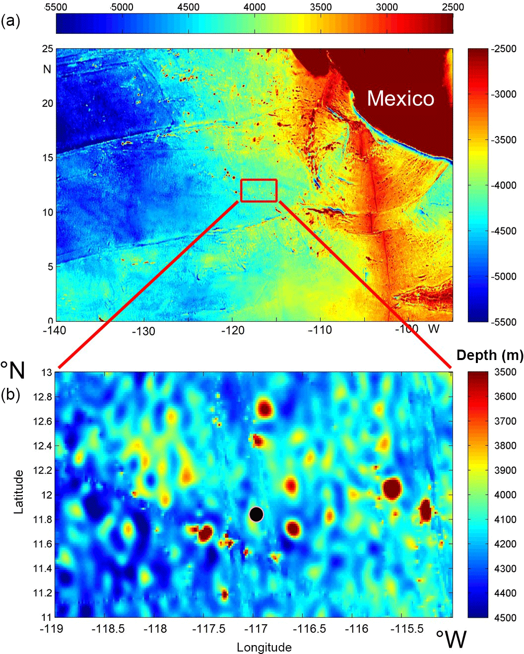
Figure 1Bathymetry map of the tropical north-east Pacific based on the Topo_9.1b 1′ version of satellite altimetry-derived data by Smith and Sandwell (1997). The black dot in panel (b) indicates mooring and CTD positions. Note the different colour ranges between the panels.
The mooring consisted of 2700 N of net top buoyancy at about 450 m from the bottom. With current speeds of less than 0.15 m s−1, the buoy did not move more than 0.1 m vertically and 1 m horizontally, as was verified using pressure and tilt sensors. The mooring line held three single-point Nortek AquaDopp acoustic current meters at 6, 207 and 408 m a.b. The middle current meter was clamped to a 0.0063 m diameter plastic-coated steel cable. To this 400 m long insulated cable 201 custom-made NIOZ4 temperature sensors were taped at 2.0 m intervals. To deploy the 400 m long instrumented cable it was spooled from a custom-made large-diameter drum with separate “lanes” for T sensors and the cable (Appendix A).
The NIOZ4 T-sensor noise level is < 0.1 mK (verified in Appendix B), and the precision is < 0.5 mK (van Haren et al., 2009; NIOZ4 is an update of NIOZ3 with similar characteristics). The sensors sampled at a rate of 1 Hz and were synchronized via induction every 4 h so that their timing mismatch was < 0.02 s and the 400 m profile was measured nearly instantaneously. As in the abyssal area temperature variations are extremely small, so severe constraints were put on the de-spiking and noise levels of the data. Under these constraints, 35 (17 % of) T sensors showed electronic timing, calibration or noise problems. Their data are no longer considered and are linearly interpolated. This low biases the estimates of turbulence parameters like dissipation rate and diffusivity from T-sensor data by about 10 %. Appendix B describes further data processing details.
During 3 days around the time of mooring deployment and 2 days after recovery, shipborne conductivity–temperature–depth (CTD) profiles were made for the monitoring of the temperature–salinity variability from 5 m below the surface to 10 m a.b. A calibrated CTD was used. The CTD data were processed using the standard procedures incorporated in the SBE software, including corrections for cell thermal mass using the parameter setting of Mensah et al. (2009) and sensor time alignment. All other analyses were performed with conservative (∼ potential) temperature (Θ), absolute salinity (SA) and density anomalies σ4 referenced to 4000 dbar using the GSW software described in IOC et al. (2010).
After the establishment of the temperature–density relationship from shipborne CTD profiles (Appendix B), the moored T-sensor data are used to estimate turbulence dissipation rate and vertical eddy diffusivity following the method of reordering potentially unstable vertical density profiles in statically stable ones, as proposed by Thorpe (1977). Here, d denotes the displacements between unordered (measured) and reordered profiles and N is computed from the reordered profiles. We use standard constant values of c1=0.8 for the Ozmidov–overturn scale factor and m1=0.2 for the mixing efficiency (e.g. Osborn, 1980; Dillon, 1982; Oakey, 1982). The validity of the latter is justified after inspection of the temperature-scalar spectral inertial subrange content (being mainly shear driven; compare to Sect. 3) and also considering the generally long averaging periods over many (> 1000) profiles. The mixing efficiency value is close to the tidal mean mixing potential observed by Cyr and van Haren (2016), also in layers in which stratification is weak. Internal waves not only induce mixing through their breaking but also allow for rapid re-stratification, making the mixing rather efficient.
The moored T-sensor data are thus much more precise and apt for using Thorpe overturning scales to estimate turbulence parameters than shipborne CTD data. Most of the concerns raised e.g. by Johnson and Garrett (2004) on this method using shipborne CTD data are not relevant here. First, instead of a single (CTD) profile, averaging is performed over 103–104 profiles, i.e. at least over the buoyancy timescale and more commonly over the inertial timescale. Second, the mooring does not move more than 0.1 m vertically and if moving it does so on a sub-inertial timescale; no corrections are needed for “ship motions” and instrumental and frame flow disturbance, as for CTD data. Third, the noise level of the moored T sensors is very low, about one-third of the high-precision sensors used in a Sea-Bird 911 CTD (Appendix B). Fourth, the environment in which the observations are made is dominated by internal wave breaking (above topography), in which turbulent mixing is generally not weak and there is a tight temperature–density relationship. Because of points three and four, complex noise reduction as in Piera et al. (2002) is not needed for moored T-sensor data. More in general for these data in such environments, Thorpe overturning scales can be solidly determined using temperature sensor data instead of more imprecise density (T- and S-sensor data), as salinity intrusions are not found important as verified. The buoyancy Reynolds number Re is used to distinguish between areas of weak, Reb < 100, and strong turbulence.
In the following, averaging over time is denoted by […] and averaging over depth range by 〈…〉. The specific averaging periods and ranges are indicated with the mean values. The vertical coordinate z is taken upward from the bottom z=0. Shear-induced overturns are visually identified as inclined S shapes in log(N) panels, while convection demonstrates more vertical columns (e.g. van Haren and Gostiaux, 2012; Fritts et al., 2016). It is noted that both types occur simultaneously, as columns exhibit secondary shear along the edges and KHi demonstrates convection in the interior core (Matsumoto and Hoshino, 2004; Li and Li, 2006).
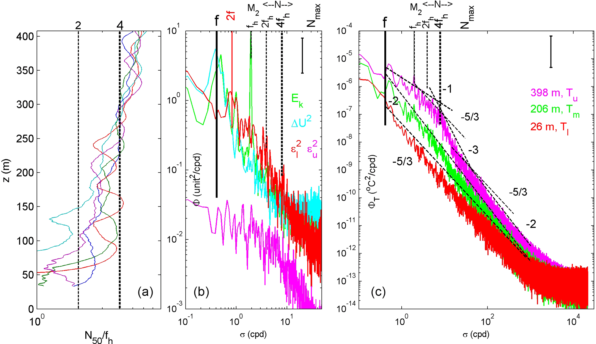
Figure 2Stratification and spectral overview. (a) Vertical profiles of buoyancy frequency scaled with the local horizontal component of the Coriolis parameter fh and smoothed over 50 dbar (∼ 50 m) from all five CTD stations to within 1 km from the mooring. The blue, green and red profiles are made around the time of mooring deployment. (b) Weakly smoothed (10 degrees of freedom, DOF) spectra of kinetic energy (upper current meter; green) and current difference (between upper and middle current meters; light blue). In red and purple are the spectra of 150 s subsampled time series of 100 m vertically averaged turbulence dissipation rates for the lower (7–107 m a.b.) and upper (307–407 m a.b.) T-sensor data segments, respectively. The inertial frequency f, fh including several higher harmonics, buoyancy frequency N including range and the semidiurnal lunar tidal frequency M2 are indicated. Nmax indicates the maximum small-scale buoyancy frequency. (c) Weakly smoothed (10 DOF) spectra of 2 s subsampled temperature data from three heights representing upper, middle and lower levels. For reference, several slopes with frequency are indicated.
High-resolution T-sensor data analysis was difficult because of the very small temperature ranges and variations of only a few mK over, especially the lower, 100 m of the observed range. This rate of variation is less than the local adiabatic lapse rate. First, a spectral analysis is performed to investigate the internal wave and turbulence range and slope appearance. Then, particular turbulent overturning aspects of internal wave breaking are demonstrated in magnifications of time–depth series. Finally, profiles of mean turbulence parameter estimates are used to focus on the extent and nature of the bottom boundary layer.
3.1 Spectral overview
The small temperature ranges are reflected in the low values of the large-scale stratification (Fig. 2a). (Salinity contributes weakly to density variations; Appendix B.) Typical buoyancy periods are 3 h, increasing to roughly 9 h in near-homogeneous layers, e.g. near the bottom. In spite of the weak stratification, the IGW band approximately between and including f and N is 1 order of magnitude wide. This IGW bandwidth is observable in spectra of turbulence dissipation rate (Fig. 2b) and temperature variance (Fig. 2c).
The T sensors have identical instrumental (white) noise levels at frequencies σ > 104 cpd and near-equal variance at sub-inertial frequencies σ < f (Fig. 2c). From the former an approximate 1 standard deviation is observed of SD ≈ ∘C; see also Appendix B. In the frequency range in between and especially for f ∼ < σ ∼ < N, the upper T-sensor data demonstrate the largest variance by up to 2 orders of magnitude at σ ≈ N compared with the lower T-sensor data. In this frequency range, the upper T-sensor spectrum has a slope of about −1 in the log–log domain, which reflects a dominance of smooth quasi-linear ocean interior IGW (van Haren and Gostiaux, 2009). Extending above this slope is a small near-inertial peak reflecting rarely observed low internal wave frequency vertical motions in weakly stratified waters (van Haren and Millot, 2005). The steep −3 roll-off at super-buoyancy frequencies σ > N is also associated with IGW. At frequencies in between and for the lower T-sensor data throughout the frequency range, a slope of is found. This reflects passive scalar turbulence dominated by shear (Tennekes and Lumley, 1972). After sufficient averaging this passive scalar turbulence is efficient (Mater et al., 2015). At intermediate depth levels and in short frequency ranges of the spectral data, slopes vary between −2 and −1. Slopes between and −1 would point at active scalar turbulence of convective mixing (Cimatoribus and van Haren, 2015), while a slope of −2 reflects fine-structure contamination (Phillips, 1971) or a saturated IGW field (Garrett and Munk, 1972).
While the upper T-sensor data contain the most variance and hence the most potential energy in the IGW band, the spectrum of estimated turbulence dissipation rate demonstrates nearly 2 orders of magnitude higher variance for the lowest T-sensor data around σ≈f (Fig. 2b). The stratification around the upper sensor supports substantial internal waves, but weak turbulence provides a flat and featureless spectrum of the dissipation rate time series. The lower layer ε spectrum shows a relative peak near σ≈2f besides one at sub-inertial frequencies, but no peaks at the inertial and semidiurnal tidal frequencies. The lack of peaks at the latter frequencies is somewhat unexpected as the kinetic energy (Fig. 2b, blue spectrum) is highly dominated by motions at M2 and, to a lesser extent, at just super-inertial 1.04f.
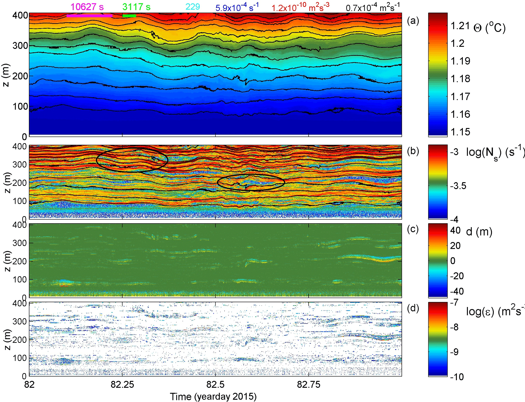
Figure 3A 1-day sample detail of moored temperature observations during relatively calm conditions (on the day of calibration in the beginning of the record). (a) Conservative temperature. The black contour lines are drawn every 0.005 ∘C. At the top from left to right are two time references indicating the mean (purple bar) and shortest (green bar) buoyancy periods found in this data detail. Values for time–depth–range–mean parameters are given by the buoyancy Reynolds number (light blue), buoyancy frequency (blue), turbulence dissipation rate (red) and turbulent eddy diffusivity (black). Errors for the latter two are to approximately within a factor of 2. (b) Logarithm of small-scale (2 dbar) buoyancy frequency from reordered temperature profiles. The black isotherms are reproduced from panel (a). (c) Thorpe displacements between raw (a) and reordered T profiles. (d) Logarithm of turbulence dissipation rate.
In contrast, the “large-scale shear” spectrum computed between current meters 200 m apart (Fig. 2b, light blue) shows a single dominant peak at just sub-inertial 0.99f, with a complete absence of a tidal peak. This reflects large quasi-barotropic vertical length scales > 400 m exceeding the mooring range at semidiurnal tidal frequencies and commonly known “small” ≤ 200 m vertical length scales at near-inertial frequencies. The large-scale shear has an average magnitude of = 2 × 10⁻⁴ s−1 for 207–408 m a.b. and 1.6 × 10⁻⁴ s−1 for 6–207 m a.b., with peak values of = 6 × 10⁻⁴ s−1 and 4 × 10⁻⁴ s−1, respectively. Considering mean 〈N〉 ≈ 5.5 × 10⁻⁴ s−1 with variations over 1 order of magnitude, the mean gradient Richardson number Ri = is larger than unity, while marginally stable conditions (Ri ≈ 0.5; Abarbanel et al., 1984) occur regularly in “bursts”. Unfortunately, higher-vertical-resolution acoustic profiler current measurements were not available to establish smaller-scale shear variations associated with higher-frequency internal waves propagating through the (large-scale) shear generated by near-inertial motions. Such smaller-scale variations in shear are expected in association with sheet-and-layer variation in stratification observed using the detailed high-resolution T sensors.
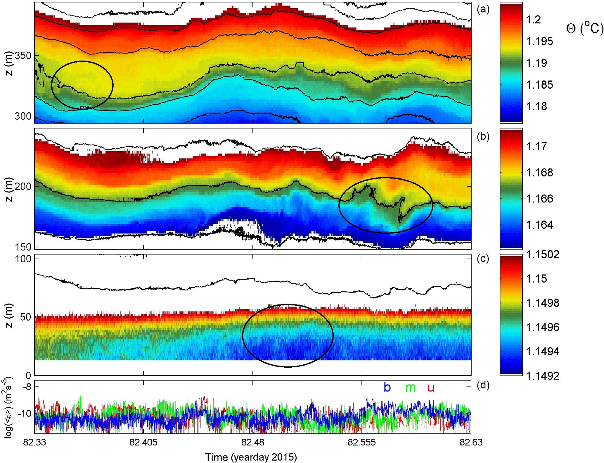
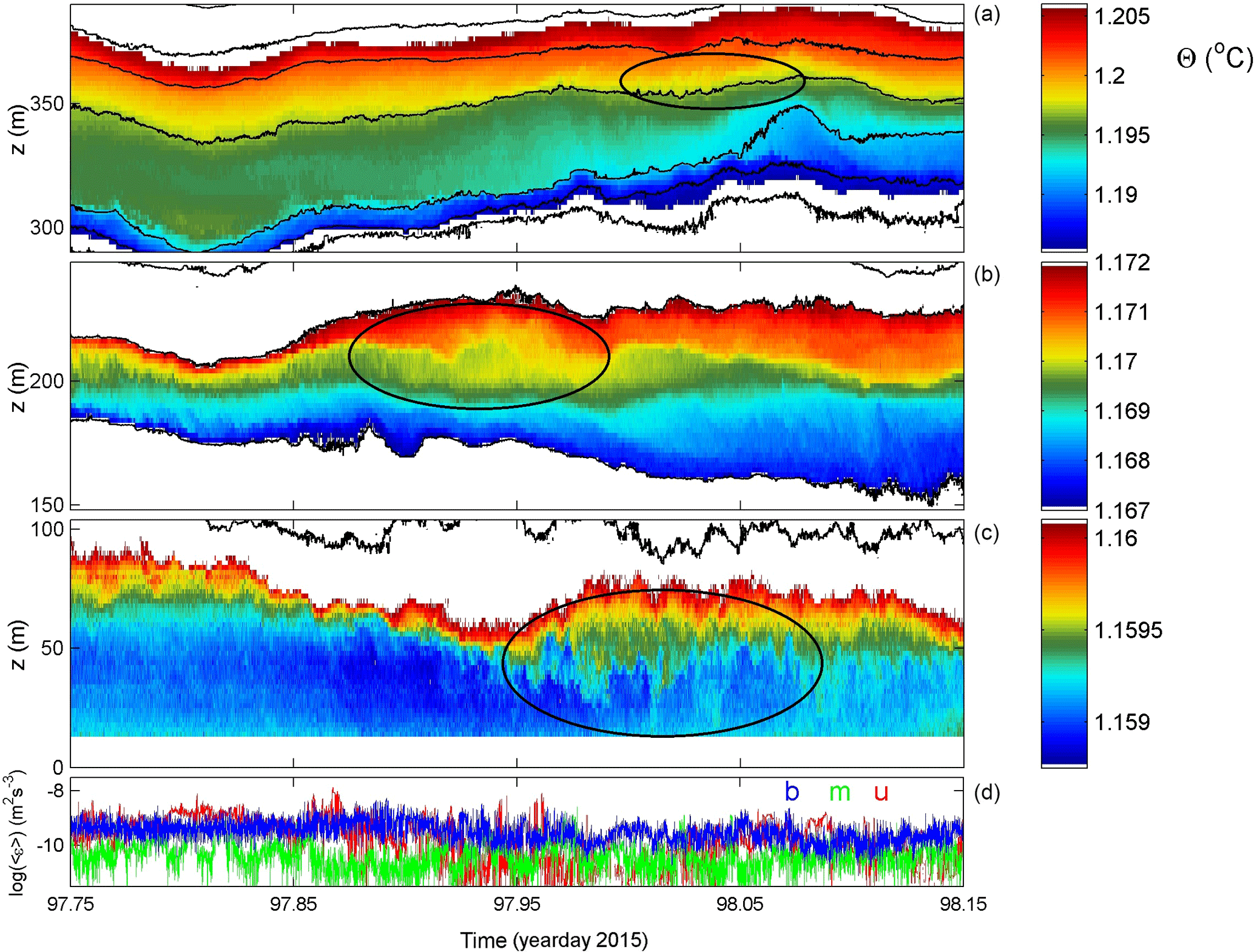
Figure 4Magnifications of Fig. 3a using different colour ranges but maintaining the 5 mK distance between isotherms. (a) Upper 100 m of the temperature sensor range (T range). (b) Approximately the middle 100 m of the T range. (c) Bottom 100 m of the T range; note the entire colour range extending over 1 mK only. (d) Time series of the logarithm of vertical mean turbulence dissipation rates from Fig. 3d for panels (a), (b) and (c) labelled u, m and b, respectively.
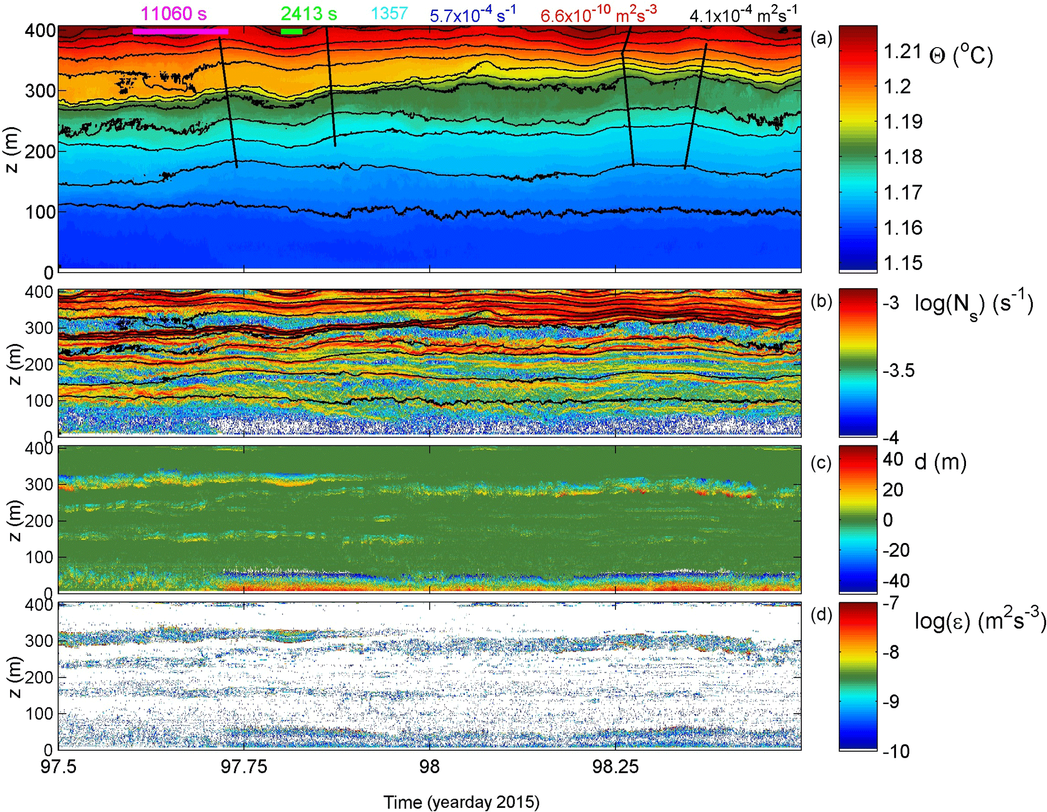
Figure 5As Fig. 3 with identical colour ranges, but for a 1-day period with more intense turbulence, especially near the bottom.
3.2 Detailed periods
The days shortly after deployment were amongst the quietest in terms of turbulence during the entire mooring period. Nevertheless, some near-bottom and interior turbulent overturning was observed occasionally (Fig. 3). For this example, averages of turbulence parameters for a 1-day time interval and 400 m vertical interval are estimated as [〈ε〉] = 1.2 ± 0.8 × 10⁻¹⁰ m2 s−3 and [〈Kz〉] = 7 ± 4 × 10⁻⁵ m2 s−1. These values are typical for open-ocean “weak turbulence” conditions although mean Reb ≈ 200. The shortest isotherm distances are observed far above the bottom (a few hundred metres; Fig. 3a), reflecting the generally stronger stratification (Fig. 3b) there. While the upper isotherms smoothly oscillate with a periodicity close to the average buoyancy period of 3.2 h and amplitudes of about 15 m, the stratification is organized in fine-scale layering throughout, except for the lower 50 m of the range. Detailed inspection of sheets (large values of small-scale Ns in Fig. 3b) demonstrates that they gain and lose strength “strain” over timescales of the buoyancy period and shorter and that they merge and deviate (e.g. around 300 m a.b. between days 82.25 and 82.5 in Fig. 3b; upper left black ellipse) also from the isotherms in association with the largest turbulent overturns (Fig. 3c) eroding them. This is reflected in non-smooth isotherms (e.g. the interior overturning near 220 m a.b. and day 82.6 in Fig. 3b; right ellipse). The patches of interior turbulent overturns, with displacements < 10 m in this example, are elongated in time–depth space, having timescales of up to the local buoyancy period but not longer. Thus, it is unlikely they represent an intrusion that can have timescales (well) exceeding the local buoyancy timescale. Considering the 0.05 m s−1 average (tidal) advection speed, their horizontal spatial extent is estimated to be about 500 m. This extent is very close to the estimated baroclinic “internal” Rossby radius of deformation Roi = m for vertical length scale H = 100 m and first mode n = 1.
The near-bottom range is different, with buoyancy periods approaching the semidiurnal period and sometimes longer. However, a permanent turbulent and homogeneous bottom boundary layer is not observed after further detailing (Fig. 4).
Examples of the upper, middle and lower 100 m of the T-sensor range are presented in magnifications with different colour ranges while maintaining the same isotherm interval of 5 mK (Fig. 4a–c). For this period, the mean flow is 0.04 ± 0.01 m s−1 towards the SE, more or less off slope of the small ridge located 5 km west of the mooring. Between these panels, the high-frequency internal wave variations decrease in frequency from upper to lower, but all panels do show overturning (e.g. as indicated by the black ellipses (around 330 m a.b. and day 82.35 in Fig. 4a, 200 m a.b. and day 82.6 in Fig. 4b, and 35 m a.b. and day 82.5 in Fig. 4c). In Fig. 4c the entire T colour range represents only 1 mK. In this depth range, the low-frequency variation in temperature and, while not related, stratification vary with a period of about 15.5 h. These variations do not have tidal-harmonic periodicity and thus do not reflect bottom friction of the dominant tidal currents. Quasi-convective overturning seems to occur after day 82.5. In the interior > 100 m a.b. most overturning seems shear induced.
The overturning phenomena are more intensely observed during a less quiescent day (Figs. 5, 6) when turbulence values are about 5 times larger and mean Reb ≈ 1400. Between 300 and 400 m a.b. isotherms remain quite smooth with near-linear internal wave oscillations (Fig. 5a, b). The lower 300 m is quasi-permanently in turbulent overturning but in specific bands only around 310 m a.b. and around 160 m a.b. (Fig. 5c, d). The latter is approximately the height of the nearest crest, still 5 km away from the mooring. RMS vertical overturn displacements are 2–3 times larger than in the previous example. Their duration is commensurate with the local buoyancy periods. The smooth upper range isotherms centred around 360 m a.b. are reflected in a 75 m, 1-day-wide range of turbulence dissipation rates below threshold (Fig. 5d). But, above and especially below, turbulent overturning is more intense; see also the detailed panels (Fig. 6). While shear-induced overturning is seen (e.g. in the black ellipses around 350 m a.b. day 98.0 (Fig. 6a) and around 200 m a.b. day 97.95; Fig. 6b), convective turbulence columns are observed (e.g. around 60 m a.b. and day 98; Fig. 6c, black ellipse). It is noted, however, that in the presented data we cannot distinguish the fine-detailed secondary overturning, e.g. shear-induced billow formation, on convection “vertical columns”. In the lower 100 m a.b., overturning occurs on large (∼ 50 m, hours) scales but also on much shorter timescales of 10 min. This results in isotherm excursions that are faster than further away from the bottom. A coupling between interior and near-bottom (turbulence and internal wave) motions is difficult to establish. For example, short-scale (high-frequency σ ≫ f) internal wave propagation > 200 m a.b. shows a downward phase (i.e. upward energy) propagation around day 97.75 (Fig. 5a) with no clear correspondence with the lower 100 m a.b. Between days 98.2 and 98.5, however, the phase propagation appears upward (downward energy propagation), with some indication for correspondence between the upper 200–400 m a.b. and lower 100 m a.b. During this period the mean 0.04 m s−1 flow was towards the west (upslope).

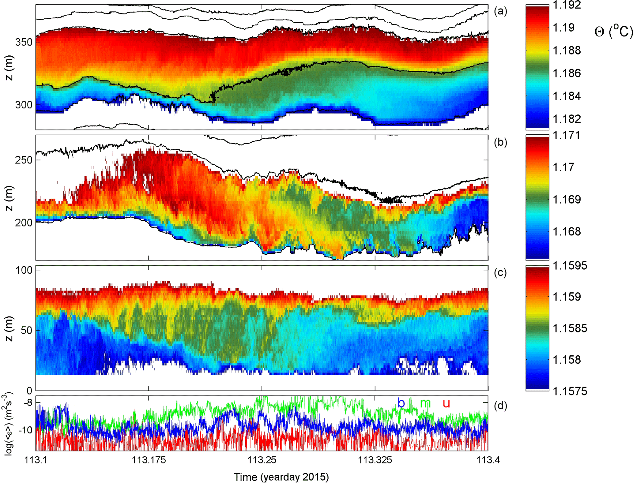
Figure 7As Fig. 3 with identical colour ranges, but for a 2-day period with occasional long shear turbulence.
Another example (of 2 days) of rather intense turbulence is given in Figs. 7 and 8, with similar average values as in the previous example. It demonstrates in particular relatively large-amplitude near-N internal waves (e.g. day 112.9, 310 m a.b.; Fig. 7a, left black ellipse) and bursts of elongated weakly sloping (slanting) shear-induced overturning (e.g. day 113.2, 210 and 50 m a.b.; Fig. 7c, black ellipses). The near-N waves appear quasi-solitary, lasting a maximum of two periods and having about 30 m trough–crest level variation. As before, the vertical phase propagation of these waves is ambiguous. In addition, very high-frequency “internal waves” around the small-scale buoyancy frequency are observed in the present example, with small amplitudes < 10 m visible in the isotherms around 300 m a.b. on day 113.1 (Fig. 7a, right black ellipse).
The interior turbulent overturning appears more intense than in preceding examples, with larger excursions of about 50 m near 200 m a.b. (Fig. 8b). This slanting layer of elongated overturns seems originally shear induced, but the overturns show clear convective properties during the observed stage. The largest duration of patches is close to the local mean buoyancy period. The entire layer demonstrates numerous shorter-timescale overturning. Crossovers, sudden changes in the vertical, are observed in isotherms from thin high-Ns above low-Ns turbulent patches to below the low-Ns patches, e.g. day 112.6 in Fig. 7b and vice versa, e.g. days 113.1 and 113.5. (Recall that small-scale Ns is computed from reordered Θ profiles.) This evidences one-sided, rather than two-sided, turbulent mixing eroding a stratified layer either from below or above.
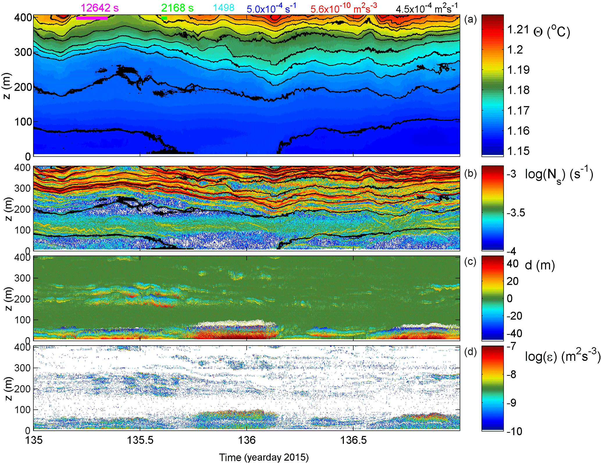
Figure 9As Fig. 3 with identical colour ranges, but for a 2-day period with some intense convective turbulence also near the bottom.
The interior shear-induced turbulent overturning seems to have some correspondence with the (top of) the near-bottom layer: on days 113.1–113.6 interior mixing is accompanied by similar near-bottom mixing. The status of the near-bottom layer (z < 75 m a.b.) switches from large-scale convective instabilities (day < 113.1) to stratified shear-induced overturning (113.1 < day < 113.6) and back to large-scale convection with probably secondary shear instabilities (day > 113.6). This is visible in the displacements (Fig. 7c) and dissipation rate (Fig. 7d), and part of it is visible in detailed temperature (Fig. 8c). The transitions between near-bottom “mixing regimes” are abruptly marked by near-bottom fronts. The mean 0.03 m s−1 flow is south-west directed (more or less on slope).
A 2-day example of a relatively intensely turbulent near-bottom layer is given in Figs. 9 and 10. Two periods about 9 h long (around days 135.9 and 136.8) and 22 h apart demonstrate > 50 m tall convective overturning extending nearly 100 m a.b. In between, large-scale shear-induced overturning dominates, with a possible correspondence with the interior in the form of a large-scale doming of isotherms and mixing in patches around day 135.4 (lasting 135.25 < day < 135.75, generally around 200 m a.b.). The doming interior isotherms are not repeated in the lowermost isotherm capping of the near-bottom layer, except perhaps for the down-going flank or front. The mean north-east flow is 0.03 m s−1 and directed more or less off slope. In this example as well as in previous ones no evidence is found for “smooth” intrusions, as demonstrated in the atmospheric DNS model by Fritts et al. (2016).
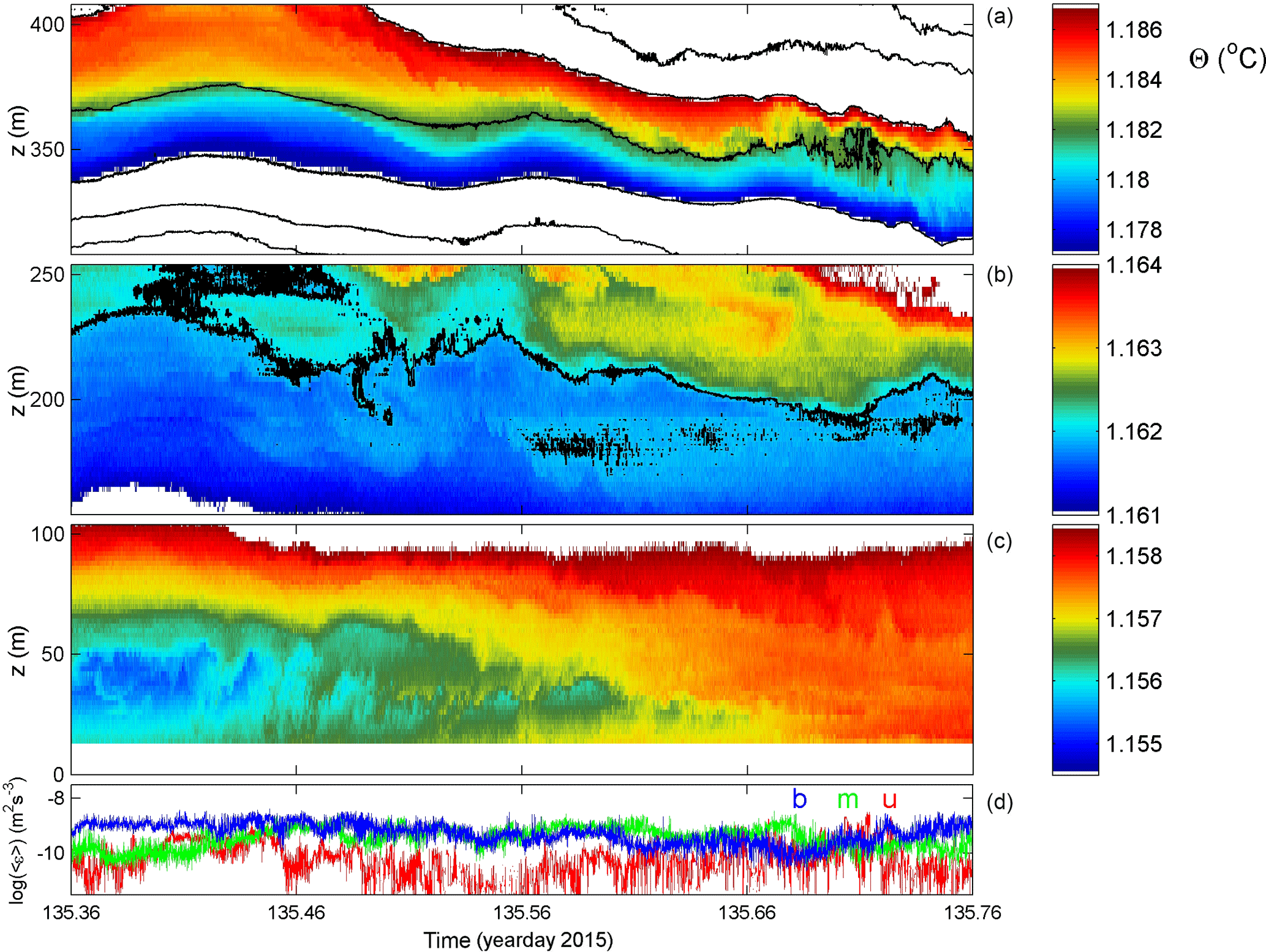
3.3 Mean profiles
The different mixing observed in the interior and near the bottom is reflected in the “mean profiles” of estimated turbulence parameters (Fig. 11a–c). These plots are constructed from patching together consecutive 1-day portions of data that are locally drift-corrected. Time-averaged values of [ε], turbulent flux (providing average [Kz]) and stratification (providing average [N]) are computed for each depth level. Averaging over a day and longer exceeds the buoyancy period even in these weakly stratified waters. It is thus considered appropriate for internal-wave-induced mixing. This may lead to some counter-intuitive averaging of displacement values greater than the local distance to the bottom at particular depths. However, it is noted that Prandtl's concept of overturn sizes never exceeding the distance to a solid boundary was based on turbulent friction of flow over a flat plate. As Tennekes and Lumley (1972) indicate, such “mixing length theoretical concept” may not be valid for flows with more than one characteristic velocity. The present area is not known for geothermal fluxes, which are also not observed in the present data. Here, the dominant turbulence generation process seems to be induced by internal waves, as the observed turbulence extends well above the layer (of the order of 10 m) of bottom friction.
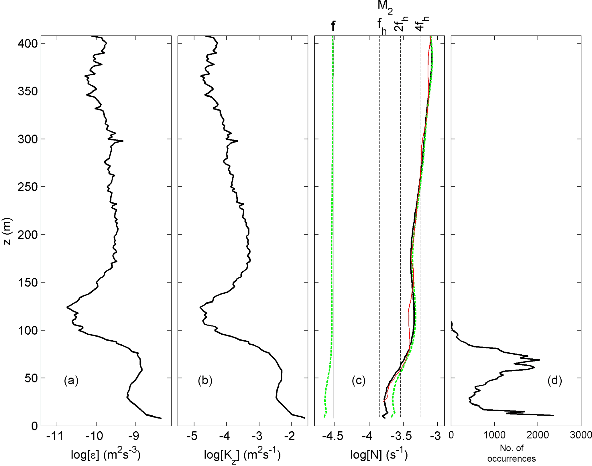
Figure 11Profiles of turbulence parameters from entire-record time-averaged estimates using 1-day drift-corrected, 150 s subsampled moored temperature data. (a) Logarithm of dissipation rate. (b) Logarithm of eddy diffusivity. (c) Logarithm of small-scale (2 dbar) buoyancy frequency from the T sensors (black) for comparison with the mean of the five CTD profiles smoothed over 50 dbar vertical intervals from Fig. 2a (red). The green dashed curves indicate the minimum (to the left of the f line) and maximum (to the right of the N profile) inertio-gravity wave bounds for meridional internal wave propagation (see text). (d) Probability density function (PDF) of the “bottom boundary layer height”, the level of the first passage of threshold N > 3 × 10⁻⁴ s−1, indicating the stratification capping the “near-homogeneous” layer from the bottom upward. Two peaks are visible, one near 10 m a.b. attributable to bottom friction and another around 65 m a.b. attributable to internal-wave-induced turbulence.
The mean dissipation rate (Fig. 11a) and diffusivity (Fig. 11b) profiles are observed to be largest between 7 and 60 m a.b., with values at least 10 times higher than in the interior. This suggests an internal wave breaking impact on sediment resuspension. Near the bottom, stratification (Fig. 11c) is low but not as weak as some 15 m higher up. At about 30 m a.b. local minima of [ε] and [Kz] are found. The average top of the weakly stratified N < s−1 ≈ 4 cpd “bottom boundary layer” is at about 65 m a.b. (Fig. 11d). This sub-maximum in the PDF distribution is broader than a second maximum closer to the bottom, near 10 m a.b. This smaller bottom boundary layer is probably induced by current friction, whereas the larger layer with an average of 65 m a.b. is probably induced by internal wave turbulence. Around 110 m a.b. the maximum of the bottom boundary layer is found with few occurrences (Fig. 11d). Around that height, the profile minimum turbulence values are observed at the depth of a weak local maximum N (Fig. 11c). This layer separates the interior turbulent mixing with a maximum around 200 m a.b. and the “near-bottom” (< 100 m a.b.) mixing. From the detailed data in Sect. 3.2 correspondence is observed between these layers, occurring at least occasionally. Considering the weaker (mean) turbulence in between, it is expected that the correspondence is communicated via internal waves and their shear. As for freely propagating IGW, its frequency band has a 1 order of magnitude width nearly everywhere, also close to the bottom (Fig. 11c). It is noted that inertial waves from all (horizontal) angles can propagate through homogeneous, weakly and strongly stratified layers, thus providing local shear (LeBlond and Mysak, 1978; van Haren and Millot, 2004).
The observed turbulence at 100 m and higher above the sea floor is mainly induced by (sub-)inertial shear and (small-scale) internal wave breaking. This confirms suggestions by Garrett and Munk (1972) about interior IGW. However, this shear is not found to decrease with N (depth) in the present data. The > 100 m a.b. depth range is termed “the interior” here, although perhaps it is not representative of the “mid-water ocean” as it is still within the height range of the surrounding hilly topography. The 130 m high ridge 5 km west of the mooring is well outside the baroclinic Rossby radius of deformation (Roi ≈ 500 m). It is not likely to influence the near-bottom turbulence here, also because no correlation is found between across-slope flow and turbulence intensity. The interior is occasionally found quiescent, with parameter values below the threshold of very weak turbulence at about 10 times molecular diffusion values. More commonly the interior is found weakly to moderately turbulent with values commensurate with open-ocean values (e.g. Gregg, 1989) following the interaction of high-frequency internal wave breaking and inertial shear.
The observed dominance of near-inertial shear at the 200 m vertical scale, the vertical separation distance between the current meters, is found far below the depths of atmospheric disturbance generation near the surface. It seems related to local generation, possibly in association with the hilly topography (St. Laurent et al., 2012; Nikurashin et al., 2014; Alford et al., 2017; Hibiya et al., 2017). Also, the 200 m vertical scale is observed to far exceed the excursion length (amplitude) of the internal waves, the scale of overturn displacements and the size of most density stratification layering. In contrast, above the Mid-Atlantic Ridge where tidal currents are only twice as energetic as near-inertial motions, the vertical length scale of tides equals that of near-inertial motions around 100–150 m (van Haren, 2007). There and in the open ocean, near-inertial motions dominate shear at shorter scales with an expected peak around 25 m (e.g. Gregg, 1989). Like in the present data, the near-inertial shear showed a shift to sub-inertial frequencies (van Haren, 2007). Because the shear magnitude was found to be concentrated in sheets of high N, it was suggested that this red shift was due to the broadening of the IGW band in low-N layers. As a result, an effective coupling between shear, stratification and the IGW band was established. Considering the similarity in sheet and layering and (large-scale) shear, such coupling is also suggested in the present observations from the deep sea over less dramatic topography.
As for a potential coupling between the interior and the observed more intense near-bottom turbulence, internal wave propagation is found in both the up and down directions. In the lower 50 m a.b. the variability in turbulence intensity, in turbulence processes of shear and convection, and in stratification demonstrates a non-smooth bottom boundary layer, perhaps better defined as an active near-bottom turbulent zone or NBTZ. As reported by Armi and D'Asaro (1980), the extent above the bottom of turbulent mixing and a near-homogeneous mixed layer varies between < 7 and 100 m a.b. with a mean of about 65 m a.b. This mean value exceeds the common frictional boundary scales that can be computed for flow over flat bottoms on a rotating sphere (Ekman, 1905), although parameterizations provide 1 order of magnitude differences: , with A the turbulent viscosity if –10−3 m2 s−1 (Fig. 11b), δ≈2.5–8 m or ; U≈0.05 m s−1, δ≈30 m (e.g. Tennekes and Lumley, 1972). Both are (substantially) less than the NBTZ found here, which thus seems to be governed by other processes such as IGW breaking. Such a relatively weak contribution of bottom friction compared to interior shear and internal wave turbulence was also observed using the instrumentation near the bottom of throughflows like the Romanche Fracture Zone (van Haren et al., 2014) and Kane Gap (van Haren et al., 2013) where current speeds are larger than ∼ 0.25 m s−1. The throughflow data form a contrast with the present observations because the near-bottom zone is stratified there despite relatively strong shear flow. They are similar in showing internal wave convection occasionally penetrating close to the bottom.
Sloping fronts are observed near the bottom in Armi and D'Asaro (1980), Thorpe (1983) and the present data. However, the isopycnal transport of mixed waters seems not to be away from the boundary as proposed in Armi and D'Asaro (1980) but rather into the NBTZ sloping downward with time (present data). This governs the variable height of the NBTZ.
Although bottom slopes were about 3 times larger in the north-east Pacific than above the Hatteras Plain, the present observations show many similarities as in Armi and D'Asaro (1980). They also show many similarities with equivalent turbulence estimates in both the interior and in the variable lower 100 m a.b. compared with those from above the central Alboran Sea, a basin of the Mediterranean Sea (van Haren, 2015), and with observations made in the south-east Pacific abyssal hill plains around −7∘7.213′ S, −88∘24.202′ W, east of the oriental Pacific Ridge (Hans van Haren, unpublished data). Thus it seems that the precise characteristics (slopes and heights) of the hilly topography are not very relevant for the observed internal wave intensity and turbulence generation as long as the bottom is not a flat plate and the hills have IGW scales. This is associated with the suggestion by Baines (2007) and Morozov (2018) that small-scale topography may prove non-negligible for internal wave generation and dissipation in comparison with large oceanic ridges, seamounts and continental slopes. After all, flat bottoms hardly exist in the ocean, depending on the length scale investigated.
The 10-fold larger turbulence intensity observed here in the NBTZ compared to the stratified interior marks a relatively extended inertial subrange. Although the near-bottom (6 m a.b.) current speeds are typically 0.05 m s−1 up to about 0.10 m s−1, the estimated turbulence intensity of 103–104 times larger than molecular diffusion is sufficient to mix materials up to 100 m a.b., the extent of observed vertical mixing in the layer adjacent to the bottom. This reflects previous observations of nephels, turbid waters of enhanced suspended materials (Armi and D'Asaro, 1980). It is expected that this material is resuspended locally, as the more intensely turbulent, steeper large-scale slopes are too far away horizontally, far beyond the baroclinic Rossby radius of deformation.
For the future, modelling may provide better insights into the precise coupling between near-inertial shear and internal wave breaking, leading to a combination of convective and shear-induced overturning. It is expected that interaction between the semidiurnal tidal current and the hilly topography may generate internal waves near the buoyancy frequency (Hibiya et al., 2017), while it remains to be investigated whether the inertial motions and shear are topographically or atmospherically driven. The one-sided shear across thin-layer stratification, as inferred from observed deviation of high-N sheets from isotherms and associated with the vertical propagation direction of internal waves, may prove important for wave breaking.
From the present high-resolution temperature sensor data moored up to 400 m above a hilly abyssal plain in the north-eastern Pacific we find an interaction between small-scale internal wave propagation, large-scale near-inertial shear and the near-bottom water phase. In an environment where semidiurnal tidal currents dominate, 200 m shear is the largest at the inertial frequency and near-bottom turbulence dissipation rates are the largest at twice the inertial frequency. Due to internal wave propagation and occasional breaking, stratification in the overlying waters is organized in thin sheets, with less stratified waters in larger layers in between, but turbulent erosion occurs asymmetrically. The average amount of turbulent overturns due to internal wave breaking here and there is equal to open-ocean turbulence, with intensities about 100 times larger than those of molecular diffusion. The high-frequency internal waves propagate to near the bottom and likely trigger 10 times larger turbulence there as shown in time-averaged vertical profiles. The result is a highly variable near-bottom turbulent zone, which may be near homogeneous over heights of less than 7 and up to 100 m above the bottom. This near-bottom turbulence is not predominantly governed by frictional flows on a rotating sphere as in Ekman dynamics that occupy a shorter range (of the order of 10 m) above the bottom. Fronts occur, as do sudden isotherm uplifts by solitary internal waves. Turbulence seems shear dominated, but occurs in parallel with convection. The shear is quasi-permanent because the dominant near-circular inertial motions have a constant magnitude. It is expected that inertial shear also dominates on shorter scales, which was not verifiable with the present current meter data, possibly added by smaller internal wave shear. In terms of the mean, turbulence dissipation rates exceed the level of 10−11 m2 s−3, except for a 30 m thick layer around 100 m a.b. Given the numerous hills distributed over the ocean floor, the present observations lend some support to their importance for internal wave turbulence generation in the ocean.
Current meter and CTD data are stored in the WDC database, PANGAEA, at https://doi.org/10.1594/PANGAEA.891476 (van Haren, 2018). The moored temperature sensor data are made available upon request to the author as they need to be computed from the raw data set for any given specific period.
The deployment of a 1-D T-sensor mooring, a thermistor string, is most commonly done for oceanographic moorings. Through the aft A frame, the top buoy is put first in the water whilst the ship is slowly steaming forward. The thermistor string is coupled between a buoy or other instrument(s) and other instrument(s) or acoustic releases before attaching the weight that is dropped in free fall. The thermistor string is put overboard through a wide, relatively large (> ∼ 0.4 m) diameter pulley about 2 m above deck or, preferably, via a smoothly rounded gunwhale (Fig. A1). Up to a 100 m length of string typically holding 100 T sensors can be put overboard manually by one or two people. In that case, the string is laid on deck in neat long loops. The deployment of a longer length of string becomes more difficult because of the weight and drag. For such strings a 1.48 m inner diameter (1.60 m OD) 1400-pin drum is constructed to safely and fully control their overboard operation (Fig. A1). The drum dimensions fit in a sea container for easy transportation. The 0.04 m high metal pins guide the cables and separate them from the T sensors in “lanes”, while allowing the cables to switch between lanes. The pins are screwed and welded in rows 0.027 and 0.023 m apart, the former sufficiently wide to hold the sensors. Up to 18 T sensors can be located in one lane before the next lane is filled. The drum has 14 double lanes and can store about 230 T sensors and 450 m of cable in one layer. The longest string deployed successfully thus far held 300 T sensors and was 600 m long, with about one-quarter of the string doubled on the drum. The doubling did not pose a problem, and the sensors were thus well separated so that entanglement did not occur. For recovery or deployment of strings holding up to 150 T sensors, a smooth surface drum is used of the same dimensions but without pins.
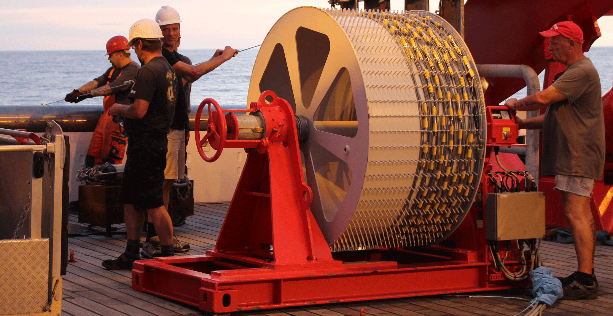
Figure A1Photo of thermistor string deployment using the instrumented cable spooling drum onboard R/V Sonne.
High-resolution T sensors can be used to estimate vertical turbulent exchange across density-stratified waters under particular constraints that are more difficult to account for under weakly stratified conditions of N < 0.1f. As in the present data the full temperature range is only 0.05∘C over 400 m, and careful calibration is needed to resolve temperatures well below the 1 mK level, at least in relative precision. Correction for instrumental electronic drift of 1–2 mK mo−1 requires shipborne high-precision CTD knowledge of the local conditions and uses the physical condition of static stability of the ocean at timescales longer than the buoyancy scale (longer than the largest turbulent overturning timescale). CTD knowledge is also needed to use temperature data as a tracer for density variations.
The NIOZ4 T-sensor noise level is nominally < 1 × 10⁻⁴ ∘C (van Haren et al., 2009; NIOZ4 is an update of NIOZ3 with similar characteristics) and thus potentially of sufficient precision. A custom-made laboratory tank can hold up to 200 T sensors for calibration against an SBE35 Deep Ocean Standards high-precision platinum thermometer to an accuracy of 2 × 10⁻⁴ ∘C over ranges of about 25 ∘C in the domain of [−4, +35] ∘C. Due to drift in the NTC resistors and other electronics of the T sensors, such accuracy can be maintained for a period of about 4 weeks after ageing. However, this period is generally shorter than the mooring period (of up to 1.5 years). During post-processing, sensor drifts are corrected by subtracting constant deviations from a smooth profile over the entire vertical range and averaged over typical periods of 4–7 days. Such averaging periods need to be at least longer than the buoyancy period to guarantee that the water column is stably stratified by definition (in the absence of geothermal heating as in the present area). Conservatively, they are generally taken longer than the local inertial period (here 2.5 days). In weakly stratified waters as in the present observations, the effect of drift is relatively so large that the smooth polynomial is additionally forced to the smoothed CTD profile obtained during the overlapping time period of data collection (Fig. B1a). In the present case, this can only be done during the first few days of deployment. Corrections for drift during other periods are made by adapting the local smooth polynomial with the difference of the (smooth average) CTD profile and the smooth polynomial of the first few days of deployment. The instrumental noise level can be verified from spectra like in Fig. 2c and, alternatively, from a near-homogeneous period and layer, here between 15 and 50 m a.b. for 1.5 h (Fig. B1b). Its standard deviation is 4 × 10⁻⁵ ∘C, which is about one-third of the standard deviation of the Sea-Bird 911 CTD–T sensor (Johnson and Garrett, 2004). The calibrated and drift-corrected T-sensor data are transferred to conservative (∼ potential) temperature (Θ) values (IOC et al., 2010) before they are used as a tracer for potential density variations δσ4 referenced to 4000 dbar, following the constant linear relationship obtained from best-fit data using all nearby CTD profiles over the mooring period and across the lower 400 m (Fig. B2). As temperature dominates density variations, this relationship's slope or
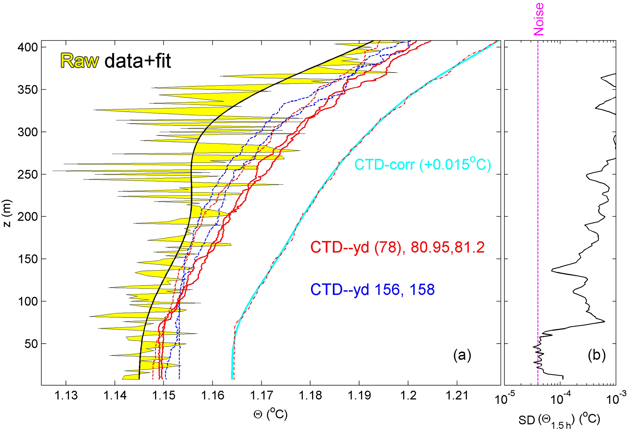
Figure B1Conservative temperature profiles with depth over the lower 400 m a.b. (a) 1-day mean moored sensor data, raw data after calibration (thin black line, yellow filled) and smooth high-order polynomial fit (thick black solid line). In red are three CTD profiles within 1 km from the mooring during the first days of deployment (two solid profiles on day 80–81 coincide in time with moored data mean), and in blue dashed are two CTD profiles after recovery of the mooring. The mean of the two solid red profiles is given by the red dashed-dot profile, 0.015∘ offset for clarity, with its smooth high-order polynomial fit in light blue to which the moored data are corrected. (b) Standard deviation of 1.5 h T-sensor data between days 80.26 and 80.32 when the layer between about 15 and 50 m a.b. is nearly homogeneous. The sensor noise level is indicated by the purple line.
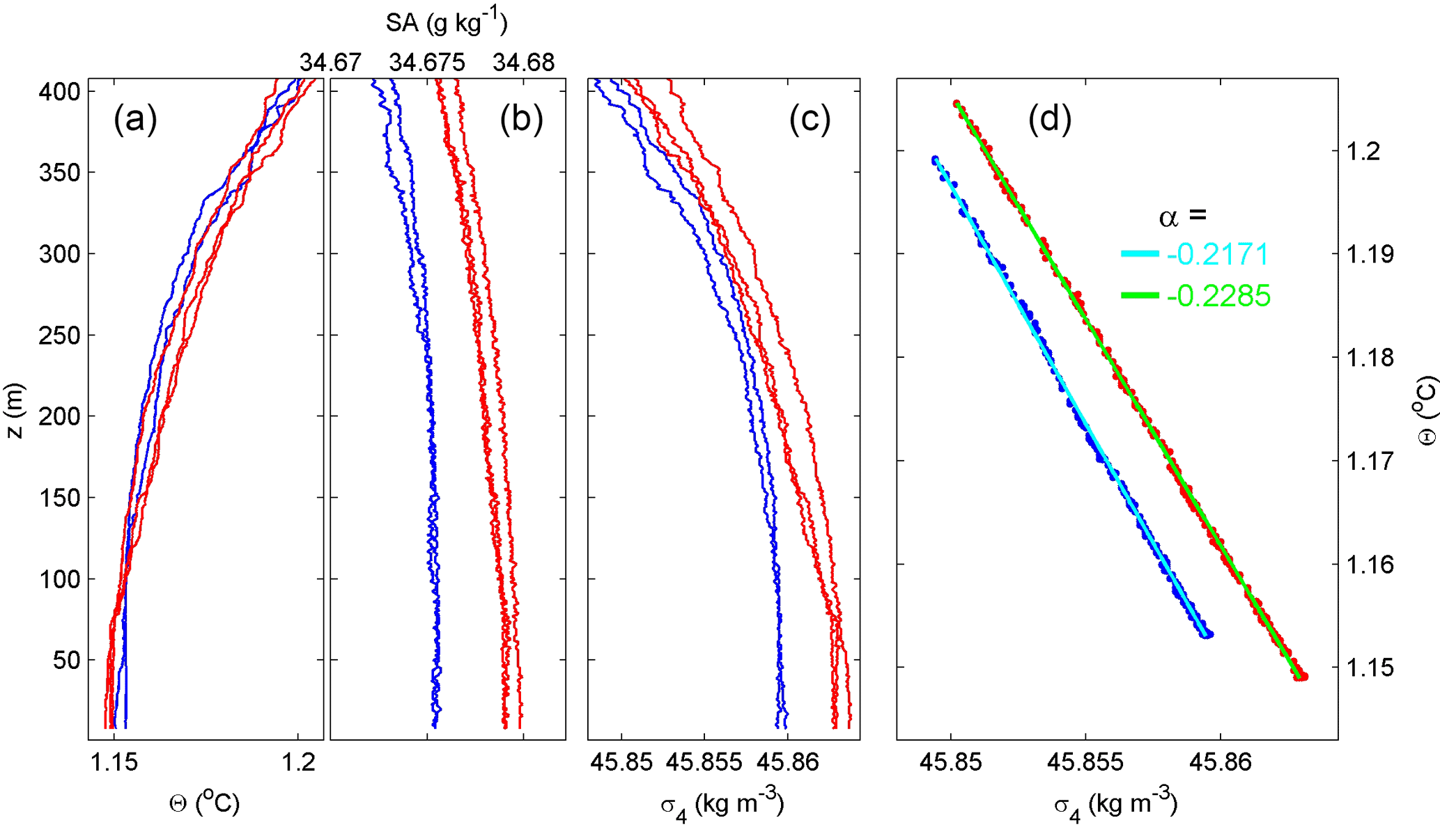
Figure B2Lower 400 m of five CTD profiles obtained near the T-sensor mooring. Red data are from around the beginning of the moored period, blue are from after recovery. (a) Conservative temperature. (b) Absolute salinity with x axis range matching the one in (a) in terms of equivalent relative contributions to density variations. The noise level is larger than for temperature. (c) Density anomaly referenced to 4000 dbar. (d) Density anomaly–conservative temperature relationship (δσ4=αδΘ). The data yielding two representative slopes after linear fit are indicated (the mean of five profiles gives < α > = −0.223 ± 0.005 kg m−3 ∘C−1).
apparent thermal expansion coefficient is kg m−3 ∘C−1 (n=5). The resolvable turbulence dissipation rate threshold averaged over a 100 m vertical range is approximately 3 × 10⁻¹² m2 s−3.
The author declares that he has no conflict of interest.
This article is part of the special issue “Assessing environmental impacts of deep-sea mining – revisiting decade-old benthic disturbances in Pacific nodule areas”. It is not associated with a conference.
I thank the master and crew of the R/V Sonne, Jens Greinert and
Annemiek Vink, for their pleasant contributions to the overboard sea
operations. Jan Blom meticulously welded the thermistor string drums,
including all of the pins. Financial support came from the Netherlands
Organization for the Advancement of Science (N.W.O.) under grant number
ALW-856.14.001 (“Ecological aspects of deep-sea mining” of the JPI Oceans
project “MiningImpact”).
Edited by: Matthias
Haeckel
Reviewed by: Eugene Morozov and one anonymous referee
Abarbanel, H. D. I., Holm, D. D., Marsden, J. E., and Ratiu, T.: Richardson number criterion for the nonlinear stability of three-dimensional stratified flow, Phys. Rev. Lett., 52, 2352–2355, 1984.
Alford, M. H. and Gregg, M. C.: Near-inertial mixing: Modulation of shear, strain and microstructure at low latitude, J. Geophys. Res., 106, 16947–16968, 2001.
Alford, M. H., MacKinnon, J. A., Simmons, H. L., and Nash, J. D.: Near-inertial internal gravity waves in the ocean, Annu. Rev. Mar. Sci., 8, 95–123, 2017.
Armi, L. and D'Asaro, E.: Flow structures of the benthic ocean, J. Geophys. Res., 85, 469–483, 1980.
Armi, L. and Millard, R. C.: The bottom boundary layer of the deep ocean, J. Geophys. Res., 81, 4983–4990, 1976.
Aucan, J., Merrifield, M. A., Luther, D. S., and Flament, P.: Tidal mixing events on the deep flanks of Kaena Ridge, Hawaii, J. Phys. Oceanogr., 36, 1202–1219, 2006.
Baines, P. G.: Internal tide generation by seamounts, Deep-Sea Res. Pt. I, 54, 1486–1508, 2007.
Bell, T. H.: Topographically generated internal waves in the open ocean, J. Geophys. Res., 80, 320–327, 1975.
Boudreau, B. P. and Jørgensen, B. B. (Eds.): The benthic boundary layer: Transport processes and biogeochemistry, Oxford University Press, Oxford, UK, 2001.
Cimatoribus, A. A. and van Haren, H.: Temperature statistics above a deep-ocean sloping boundary, J. Fluid Mech., 775, 415–435, 2015.
Cyr, F. and van Haren, H.: Observations of small-scale secondary instabilities during the shoaling of internal bores on a deep-ocean slope, J. Phys. Oceanogr., 46, 219–231, 2016.
Dillon, T. M.: Vertical overturns: A comparison of Thorpe and Ozmidov length scales, J. Geophys. Res., 87, 9601–9613, 1982.
Ekman, V. W.: On the influence of the Earth's rotation on ocean-currents, Ark. Math. Astron. Fys., 2, 1–52, 1905.
Eriksen, C. C.: Observations of internal wave reflection off sloping bottoms, J. Geophys. Res., 87, 525–538, 1982.
Fritts, D. C., Wang, L., Geller, M. A., Lawrence, D. A., Werne, J., and Balsley, B. B.: Numerical modeling of multiscale dynamics at a high Reynolds number: Instabilities, turbulence, and an assessment of Ozmidov and Thorpe scales, J. Atmos. Sci., 73, 555–578, 2016.
Gerkema, T., Zimmerman, J. T. F., Maas, L. R. M., and van Haren, H.: Geophysical and astrophysical fluid dynamics beyond the traditional approximation, Rev. Geophys., 46, RG2004, https://doi.org/10.1029/2006RG000220, 2008.
Garrett, C. and Munk, W.: Oceanic mixing by breaking internal waves, Deep-Sea Res., 19, 823–832, 1972.
Gregg, M. C.: Scaling turbulent dissipation in the thermocline, J. Geophys. Res., 94, 9686–9698, 1989.
Hibiya, T., Ijichi, T., and Robertson, R.: The impacts of ocean bottom roughness and tidal flow amplitude on abyssal mixing, J. Geophys. Res., 122, 5645–5651, https://doi.org/10.1002/2016JC012564, 2017.
Hollister, C. D. and McCave, I. N.: Sedimentation under deep-sea storms, Nature, 309, 220–225, 1984.
IOC, SCOR, and IAPSO: The international thermodynamic equation of seawater – 2010: Calculation and use of thermodynamic properties, Intergovernmental Oceanographic Commission, Manuals and Guides No. 56, UNESCO, Paris, France, 2010.
Johnson, H. L. and Garrett, C.: Effects of noise on Thorpe scales and run lengths, J. Phys. Oceanogr., 34, 2359–2372, 2004.
Lazier, J. R. N.: Temporal changes in some fresh water temperature structures, J. Phys. Oceanogr., 3, 226–229, 1973.
LeBlond, P. H. and Mysak, L. A.: Waves in the Ocean, Elsevier, New York, 1978.
Li, S. and Li, H.: Parallel AMR code for compressible MHD and HD equations, T-7, MS B284, Theoretical division, Los Alamos National Laboratory, available at: http://citeseerx.ist.psu.edu/viewdoc/summary;jsessionid=1548A302FD5C2B1DFAC1BA7A5E70605F?doi=10.1.1.694.3243 (last access: 16 July 2018), 2006.
Lochte, K.: Bacterial Standing Stock and Consumption of Organic Carbon in the Benthic Boundary Layer of the Abyssal North Atlantic, in: Deep-Sea Food Chains and the Global Carbon Cycle, edited by: Rowe, G. T. and Pariente, V., Kluwer, Dordrecht, 1–10, 1992.
Mater, B. D., Venayagamoorthy, S. K., St. Laurent, L., and Moum, J. N.: Biases in Thorpe scale estimates of turbulence dissipation. Part I: Assessments from large-scale overturns in oceanographic data, J. Phys. Oceanogr., 45, 2497–2521, 2015.
Matsumoto, Y. and Hoshino, M.: Onset of turbulence by a Kelvin-Helmholtz vortex, Geophys. Res. Lett., 31, L02807, https://doi.org/10.1029/2003GL018195, 2004.
Mensah, V., Le Menn, M., and Morel, Y.: Thermal mass correction for the evaluation of salinity, J. Atmos. Ocean. Tech., 26, 665–672, 2009.
Morozov, E. G.: Semidiurnal internal wave global field, Deep-Sea Res. Pt. I, 42, 135–148, 1995.
Morozov, E. G.: Internal Tides: Observations, analysis and modeling; A Global View, Springer, Berlin, 2018.
Nikurashin, M., Ferrari, R., Grisouard, N., and Polzin, K.: The impact of finite-amplitude bottom topography on internal wave generation in the southern ocean, J. Phys. Oceanogr., 44, 2938–2950, 2014.
Oakey, N. S.: Determination of the rate of dissipation of turbulent energy from simultaneous temperature and velocity shear microstructure measurements, J. Phys. Oceanogr., 12, 256–271, 1982.
Osborn, T. R.: Estimates of the local rate of vertical diffusion from dissipation measurements, J. Phys. Oceanogr., 10, 83–89, 1980.
Phillips, O. M.: On spectra measured in an undulating layered medium, J. Phys. Oceanogr., 1, 1–6, 1971.
Piera, J., Roget, E., and Catalan, J.: Patch identification in microstructure profiles: A method based on wavelet denoising and Thorpe displacement analysis, J. Atmos. Ocean. Tech., 19, 1390–1402, 2002.
Smith, W. H. F. and Sandwell, D. T.: Global seafloor topography from satellite altimetry and ship depth soundings, Science, 277, 1957–1962, 1997.
St. Laurent, L. C., Garabato, A. C. N., Ledwell, J. R., Thurnherr, A. M., Toole, J. M., and Watson, A. J.: Turbulence and diapycnal mixing in Drake Passage, J. Phys. Oceanogr., 42, 2143–2152, 2012.
Tennekes, H. and Lumley, J. L.: A first course in Turbulence, MIT Press, Cambridge, 1972.
Thorpe, S. A.: Turbulence and mixing in a Scottish loch, Philos. T. R. Soc. Lond., 286, 125–181, 1977.
Thorpe, S. A.: Benthic observations on the Madeira abyssal plain: Fronts, J. Phys. Oceanogr., 13, 1430–1440, 1983.
Thorpe, S. A.: Models of energy loss from internal waves breaking in the ocean, J. Fluid Mech., 836, 72–116, 2018.
van Haren, H.: Inertial and tidal shear variability above Reykjanes Ridge, Deep-Sea. Res. Pt. I, 54, 856–870, 2007.
van Haren, H.: Impressions of the turbulence variability in a weakly stratified, flat-bottom deep-sea “boundary layer”, Dynam. Atmos. Oceans, 69, 12–25, 2015.
van Haren, H.: CTD and current meter data from SONNE cruises SO239 and SO240, PANGAEA, https://doi.org/10.1594/PANGAEA.891476, 2018.
van Haren, H. and Gostiaux, L.: High-resolution open-ocean temperature spectra, J. Geophys. Res., 114, C05005, https://doi.org/10.1029/2008JC004967, 2009.
van Haren, H. and Gostiaux, L.: Detailed internal wave mixing above a deep-ocean slope, J. Mar. Res., 70, 173–197, 2012.
van Haren, H. and Millot, C.: Rectilinear and circular inertial motions in the Western Mediterranean Sea, Deep-Sea Res. Pt. I, 51, 1441–1455, 2004.
van Haren, H. and Millot, C.: Gyroscopic waves in the Mediterranean Sea, Geophys. Res. Lett., 32, L24614, https://doi.org/10.1029/2005GL023915, 2005.
van Haren, H., Laan, M., Buijsman, D.-J., Gostiaux, L., Smit, M. G., and Keijzer, E.: NIOZ3: independent temperature sensors sampling yearlong data at a rate of 1 Hz, IEEE J. Ocean. Eng., 34, 315–322, 2009.
van Haren, H., Morozov, E., Gostiaux, L., and Tarakanov, R.: Convective and shear-induced turbulence in the deep Kane Gap, J. Geophys. Res., 118, 5924–5930, https://doi.org/10.1002/2013JC009282, 2013.
van Haren, H., Gostiaux, L., Morozov, E., and Tarakanov, R.: Extremely long Kelvin-Helmholtz billow trains in the Romanche Fracture Zone, Geophys Res. Lett., 41, 8445–8451, https://doi.org/10.1002/2014GL062421, 2014.
Wimbush, M.: Temperature gradient above the deep-sea floor, Nature, 227, 1041–1043, 1970.
- Abstract
- Introduction
- Methods and data handling
- Observations
- Discussion
- Conclusions
- Data availability
- Appendix A: Thermistor string drum: a dedicated instrumented cable spool
- Appendix B: Temperature sensor data processing in weakly stratified waters
- Competing interests
- Special issue statement
- Acknowledgements
- References