the Creative Commons Attribution 4.0 License.
the Creative Commons Attribution 4.0 License.
 | 21 Dec 2020
Migrating tide climatologies measured by a high-latitude array of SuperDARN HF radars
Willem E. van Caspel
Patrick J. Espy
Robert E. Hibbins
John P. McCormack
This study uses hourly meteor wind measurements from a longitudinal array of 10 high-latitude SuperDARN high-frequency (HF) radars to isolate the migrating diurnal, semidiurnal, and terdiurnal tides at mesosphere–lower-thermosphere (MLT) altitudes. The planetary-scale array of radars covers 180∘ of longitude, with 8 out of 10 radars being in near-continuous operation since the year 2000. Time series spanning 16 years of tidal amplitudes and phases in both zonal and meridional wind are presented, along with their respective annual climatologies. The method to isolate the migrating tides from SuperDARN meteor winds is validated using 2 years of winds from a high-altitude meteorological analysis system. The validation steps demonstrate that, given the geographical spread of the radar stations, the derived tidal modes are most closely representative of the migrating tides at 60∘ N. Some of the main characteristics of the observed migrating tides are that the semidiurnal tide shows sharp phase jumps around the equinoxes and peak amplitudes during early fall and that the terdiurnal tide shows a pronounced secondary amplitude peak around day of year (DOY) 265. In addition, the diurnal tide is found to show a bi-modal circular polarization phase relation between summer and winter.


Atmospheric tides are global-scale waves excited primarily by radiative and latent heating effects in the troposphere and stratosphere (Chapman and Lindzen, 2012). The tides have a latitudinal spherical harmonic structure (termed Hough modes) and longitudinal zonal wavenumber (S) structure, and in the absence of dissipation their amplitudes increase exponentially with altitude due to the decreasing density of the atmosphere. In the mid- to high-latitude mesosphere–lower-thermosphere (MLT), tides are an important driver of short- and long-term variability in the winds, temperatures, and densities (Smith, 2012). The migrating diurnal (DW1; for diurnal, westward, S = 1), semidiurnal (SW2), and terdiurnal (TW3) tides are most closely tied to the daily insolation cycle, following the apparent motion of the sun with periods of oscillation of 24, 12, and 8 h, respectively. Non-migrating tides are waves whose periods of oscillation are also an integer fraction of a solar day but whose phase velocities are not sun-synchronous.
Observations capable of separating the longitudinal structure of the migrating tides from the non-migrating components have remained sparse, with the exception of satellites (e.g., Garcia et al., 2005; Ortland, 2017; Pancheva and Mukhtarov, 2011). Typical drawbacks associated with satellite measurements arise due to constraints imposed by asynoptic sampling (Salby, 1982), including slow local time precession and yaw cycle maneuvers. Single station tidal measurements using medium-frequency (MF), high-frequency (HF), or very-high-frequency (VHF) radars have been numerous (Reid, 2015), but because they lack longitudinal coverage, the migrating and non-migrating tides are aliased to a single local wave with an integer fraction of a solar day period. Such spatial aliasing is especially problematic when migrating and non-migrating tides are known to have different seasonal cycles (Sakazaki et al., 2018; Hibbins et al., 2019). A planetary-scale longitudinal chain of time-synchronized measurements can potentially bypass most, if not all, of the drawbacks associated with satellite and single station tide measurements, albeit along a single latitude. The array of SuperDARN (SD) radars used in this study is unique in that it covers 180∘ of longitude along a latitude band centered around 60∘ N and that 8 of the 10 radars have been providing hourly meteor wind measurements of the MLT near-continuously since the year 2000. As a result of the simultaneous temporal and spatial sampling by the SD radars, unambiguous amplitudes and phases of the migrating diurnal, semidiurnal, and terdiurnal tides can be isolated.
The following section gives a description of the data and method used to extract the migrating tides from the SD meteor winds. Section 3 presents time series spanning 16 years of hourly tidal amplitudes and phases in both the zonal and meridional winds, in addition to their respective annual climatologies. The method to extract migrating tides from the SD meteor winds is validated in Sect. 4 by means of sampling experiments with winds obtained from the NAVGEM-HA (Navy Global Environmental Model – High Altitude) meteorological analysis system, addressing the geographical spread and changing availability in time of the SD radars. Lastly, the results are discussed in Sect. 5.
2.1 SuperDARN meteor winds
Figure 1 shows the geographical location and data availability between the years 2000 and 2016 of the 10 SD radars used in this study. The SD radars operate in a 10–15 MHz frequency band and are designed to measure ionospheric E- and F-region plasma phenomena. However, they also detect near-range meteor echoes in the first four range gates that can be used to determine neutral horizontal wind velocities (Hall et al., 1997). The phase shift of the return signal of each meteor echo is a measure of the component of the neutral wind velocity along the line of sight. An hourly mean horizontal wind vector is constructed from the aggregate line-of-sight wind vectors, over a 45∘ spread in azimuth, using a singular value decomposition (SVD). While the line-of-sight velocities are typically very well defined (errors below 1 m s−1, Chisham and Freeman, 2013), the SVD is applied only to line-of-sight velocities with a signal-to-noise ratio greater than 3.0 dB and a spectral width of at most 25 m s−1, to reduce contamination by sources such as auroral and sporadic E-region echoes. In addition to a hourly horizontal wind vector, the SVD also yields the standard deviation of the hourly winds, which typically ranges between 5 and 15 m s−1 for the meridional wind and between 10 and 30 m s−1 for the zonal wind. The seasonal mean vertical distribution of meteor echoes as observed by the SD radars is a Gaussian centered on 102–103 km altitude, extending from approximately 75 to 125 km altitude with a full width at half maximum of 25–35 km (Chisham and Freeman, 2013; Chisham, 2018). The SD meteor winds therefore represent a broad vertical average, which in earlier studies has been found to best correlate with neutral winds measured by traditional MF and meteor radars around 95 km altitude (Hall et al., 1997; Arnold et al., 2003).
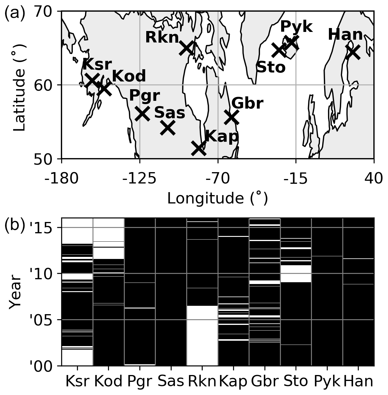
Figure 1Abbreviated names and geographic locations (a) and time of operation between the years 2000 and 2016 (black marking b) of the SuperDARN radars used in this study.
On average each hourly SD meteor wind measurement is based on ∼ 700 meteor echoes. Before extracting the migrating tides, however, measurements based on fewer than 75 meteor echoes are discarded, as are those resulting from non-standard modes of operation. The latter amounts to discarding winds with absolute values above 100 m s−1 and winds fitted with a zero standard deviation (following Hibbins and Jarvis, 2008). The lower limit on the number of meteor echoes is to ensure quality of the fitted winds. Caution has been taken to ensure that no spurious tidal signals are introduced by the quality check, which may arise due to the diurnal cycle in meteor detections. This was verified by replacing all remaining data points with a value of 1 m s−1 and then performing spectral analysis as outlined in the following section, to confirm that tidal spectral contamination remains negligibly small.
2.2 Fourier analysis
The amplitude and phase of DW1, SW2, and TW3 are calculated by least-squares fitting the function G(λ,t) in both space and time, where G(λ,t) represents the migrating tides along with a mean wind, given by
where represent DW1, SW2, and TW3, respectively, h−1; λ is the geographic longitude in radians; and G0 is the mean wind. The time development is determined by fitting G(λ,t) over a 10 d window that is stepped forward in time with hourly steps over the range of available data. A 10 d window length is chosen such that each fit contains a proportionally sufficient number of data points to reliably extract the seasonal characteristics of the tides, without overly smoothing short-term variability.
The equidistant longitudinal spread of measurements is optimized over the range of available data to prevent skewing the fit to any particular longitude sector. To that end, for the radar pairs closely spaced in longitude, (Ksr, Kod), (Rnk, Kap), and (Sto, Pyk), only one of each of the pairs' measurements is used in the fit to Eq. (1), even if data are available for both. After performing the quality check and optimizing the longitudinal spread, fits are rejected if fewer than 960 hourly data points are present over the 10 d period, corresponding to an average continuous uptime of at least four radar stations. As a result of requiring a minimum of 960 hourly data points in each fit to Eq. (1), the estimated uncertainties on the fitted parameters become negligibly small (on the order of 0.5 m s−1 for the tidal amplitudes when employing the standard deviations of the hourly winds as an estimate of the measurement errors).
2.3 NAVGEM-HA
NAVGEM-HA is a data assimilation and modeling system that extends from the surface to the lower thermosphere. In addition to standard operational meteorological observations in the troposphere and stratosphere, NAVGEM-HA assimilates satellite-based observations of temperature, ozone, and water vapor in the stratosphere, mesosphere, and lower thermosphere (McCormack et al., 2017). NAVGEM-HA output is on a 1∘ latitude and longitude grid with a temporal frequency of 3 h, staying above the spatial and temporal Nyquist frequency of the tides studied in this work. For comparison with ground-based instruments, vertical profiles of NAVGEM-HA analyzed winds and temperatures are converted from the model vertical grid in geopotential altitude to a geometric altitude grid. To date, NAVGEM-HA winds and tides have been shown to be in good agreement with ground-based meteor radar observations (McCormack et al., 2017; Eckermann et al., 2018; Laskar et al., 2019; Stober et al., 2020) and with independent satellite-based wind observations as reported in Dhadly et al. (2018). In the present study we employ NAVGEM-HA analyzed winds at 82.5 km altitude, staying below altitudes where effects of increased numerical diffusion imposed at the NAVGEM-HA upper boundary may impact the tides, to validate the method of extracting migrating tidal signatures from the SD meteor wind data.
3.1 Sixteen-year time series
Figures 2 and 3 show the amplitudes and phases of the DW1, SW2, and TW3 tides retrieved from SD zonal and meridional meteor winds between the years 2000 and 2016. Here the phases are shown as the local time of maximum (LTOM), and phases for tidal amplitudes less than 1.5 m s−1 are not shown for sake of clarity.
SW2 shows a strongly repeatable seasonal cycle, where amplitudes peak around early fall (September–October) and mid-winter (December–January) and where sharp phase jumps occur around spring and fall equinox. The early fall amplitude maximum of SW2 typically reaches values between 19 and 25 m s−1. In contrast, the mid-winter amplitude maximum typically lies between 10 and 14 m s−1. SW2 consistently reaches amplitude minima coincident with the equinoctial phase jumps. While the amplitude and phase progression between the zonal and meridional components are nearly identical, meridional amplitudes can at times be 4–5 m s−1 larger, especially during mid-summer (June–July). In terms of its absolute phase separation, the meridional component of SW2 is found to lead the zonal component by 2.48 h on average, giving it a 32 min offset relative to a perfect circular polarization.
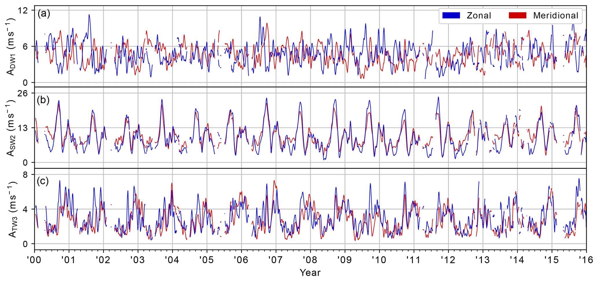
Figure 2Amplitude of DW1 (a), SW2 (b), and TW3 (c) in SuperDARN zonal (red) and meridional (blue) meteor winds between the years 2000 and 2016.
TW3 also shows a strongly repeatable seasonal cycle, where a broad amplitude maximum is centered on the winter half-year (October–March) and where the phase begins to shift to a later time starting October, stabilizes around the turn of the year, and then shifts back to its pre-winter value up to March. Wintertime amplitudes typically reach values between 4 and 6 m s−1, whereas the tide is nearly non-existent throughout summer. At times the amplitude of TW3 can surpass those of SW2 and DW1, in particular around fall equinox, when SW2 reaches a minimum. In addition, a pronounced secondary TW3 amplitude peak is found near day of year (DOY) 265, which can be more clearly seen in the climatology presented in the next section. This peak is most pronounced in the zonal wind, where it can reach amplitudes in the range of 4–7 m s−1. In terms of its phase, TW3 is found to be nearly circularly polarized during times when the wave has an appreciable amplitude, with the meridional component leading the zonal component by 1.98 h on average.
DW1 shows considerably more short-term and interannual variability in its amplitude, phase, and between the zonal and meridional components. This is reflected in the correlation coefficient of between the time series of hourly zonal and meridional amplitudes of DW1, whereas for SW2 and TW3 this is r=0.90 and r=0.66, respectively. There is, however, a clear seasonal cycle present in both the amplitude and phase of DW1, which can be more clearly seen in the climatology presented in the next section.
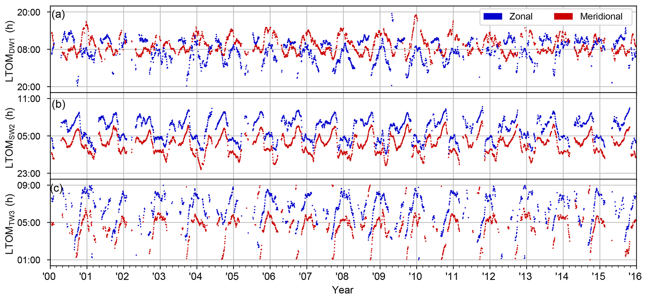
Figure 3Phase of DW1 (a), SW2 (b), and TW3 (c) in SuperDARN zonal (red) and meridional (blue) meteor winds between the years 2000 and 2016. Phases are plotted as the local time of maximum (LTOM). Only phases for when tidal amplitudes are greater than 1.5 m s−1 are shown for clarity.
3.2 Climatologies
Figure 4 shows the yearly amplitude and phase climatologies of DW1, SW2, and TW3 based on the amplitudes and phases presented in the previous section. The climatologies are constructed by calculating the mean amplitude and phase for each DOY, where the mean phase is calculated using the circular mean (Fisher, 1995). The shaded area represents the standard deviation around the climatological mean amplitude and serves as a measure of year-to-year variability.
For the zonal (meridional) component, the climatological amplitude of SW2 in early fall and mid-winter peaks at 20.7 (18.8) m s−1 and 12.4 (12.4) m s−1, respectively. Variability around the climatological mean of SW2 is largely constant throughout the year, with an average standard deviation of 2.2 (2.0) m s−1. For TW3, wintertime zonal (meridional) amplitudes peak at 4.4 (5.1) m s−1, while the DOY 265 amplitude peaks at 5.3 (4.1) m s−1. The average standard deviation of the amplitude of TW3 is 1.0 (0.9) m s−1, while variability around the climatological mean is highest coincident with the amplitude peak at DOY 265 by 1.7 (1.4) m s−1.
The climatology of DW1 stands out in that amplitudes in the meridional wind broadly tend to maximize around 6.7 m s−1 near the equinoxes, whereas those in the zonal wind maximize around 6.7 m s−1 near the solstices. In addition, the climatological phase shows a circular polarization where the zonal component leads the meridional by approximately 6 h during the winter half-year but lags it by approximately 6 h during the summer half-year. The climatological phase thus shows a bi-modal circular polarization, with the polarization flipping sign broadly between summer and winter. Variability around the climatological amplitude of the zonal (meridional) component of DW1 stays largely constant throughout the year, with an average standard deviation of 1.6 (1.3) m s−1.
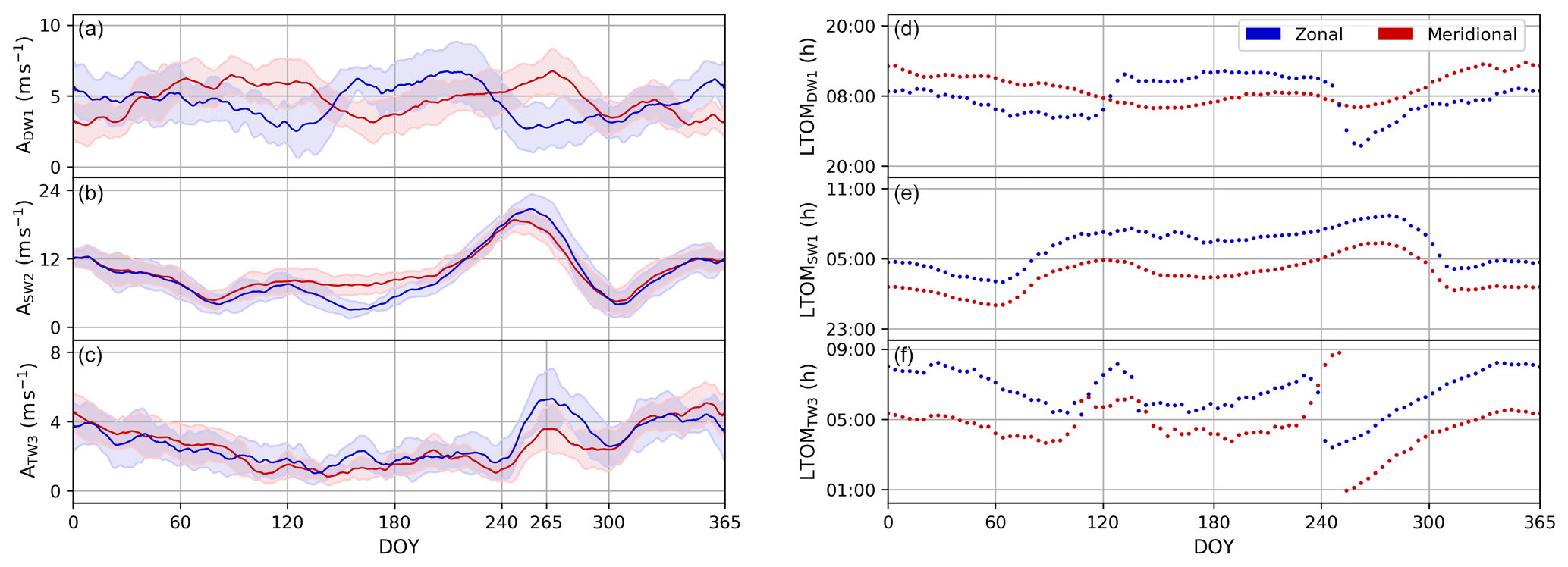
Figure 4Climatologies of the amplitude (a–c) and phase (d–f) of the DW1 (a), SW2 (b), and TW3 (c) based on SuperDARN meridional (red) and zonal (blue) meteor winds between the years 2000 and 2016. Shading marks the standard deviation around the climatological mean. The amplitude of TW3 on DOY 265, referenced extensively in the text, is indicated in (c).
In this section sampling experiments with NAVGEM-HA are used to validate the method to extract migrating tides from the longitudinal chain of SD meteor wind measurements. The sampling experiments seek to address the geographical spread of the SD stations as well as the spatial sampling variations due to the changing availability of the individual stations with time (as shown in Fig. 1). Cross-contamination errors arising from the geographical spread of the SD stations are expected to be large relative to the error propagating from any individual measurement uncertainties, since each tidal fit includes at least 960 hourly data points, as discussed in Sect. 2.2.
4.1 Geographical spread
To address the geographical spread of the SD stations, migrating tides (Eq. 1) are fitted to NAVGEM-HA meridional winds sampled at the locations of available SD measurements (NAVGEM-SD), after quality checking and optimizing the longitudinal spread as discussed in Sect. 2.2. These are then compared against those fitted to a full longitude circle of data taken along 60∘ N (NAVGEM-360). Fits along a full longitude circle are orthogonal to any other longitudinal waves and so form a benchmark of the “true” migrating tides. As with the fits to SD, a 10 d time window is used where the window is now stepped forward in three hourly steps to accommodate the temporal resolution of NAVGEM-HA.
Figure 5 shows the migrating tides derived from NAVGEM-SD and NAVGEM-360 for the years 2014 and 2015, demonstrating that there is no structural deviation between the two for all three tidal components. The largest amplitude deviations remain incidental, whereas the phases are in close agreement at all times. On average, the phase difference between NAVGEM-SD and NAVGEM-360 is 5.9, 5.6 and 6.0 min for DW1, SW2, and TW3, respectively. The geographical spread of the SD radars is therefore concluded to not lead to significant cross-contamination errors between the migrating tides.
The corresponding tides measured by the array of SD radars are also shown in Fig. 5 (green curves). These are, however, not intended to serve as a detailed comparison between the modeled and observed tides. For such a comparison the top level of the NAVGEM-HA system would have to be extended past the vertical extent of the SD meteor echo distribution (∼ 125 km), which is beyond the scope of the current work. Nevertheless, the SW2 and TW3 tides from SD and NAVGEM-HA at 82.5 km share similar characteristics in their seasonal amplitude and phase cycle, supporting the use of NAVGEM-HA to validate the SD tidal analysis method. A possible reason for the difference between the modeled and observed DW1 tide is discussed in Sect. 5.
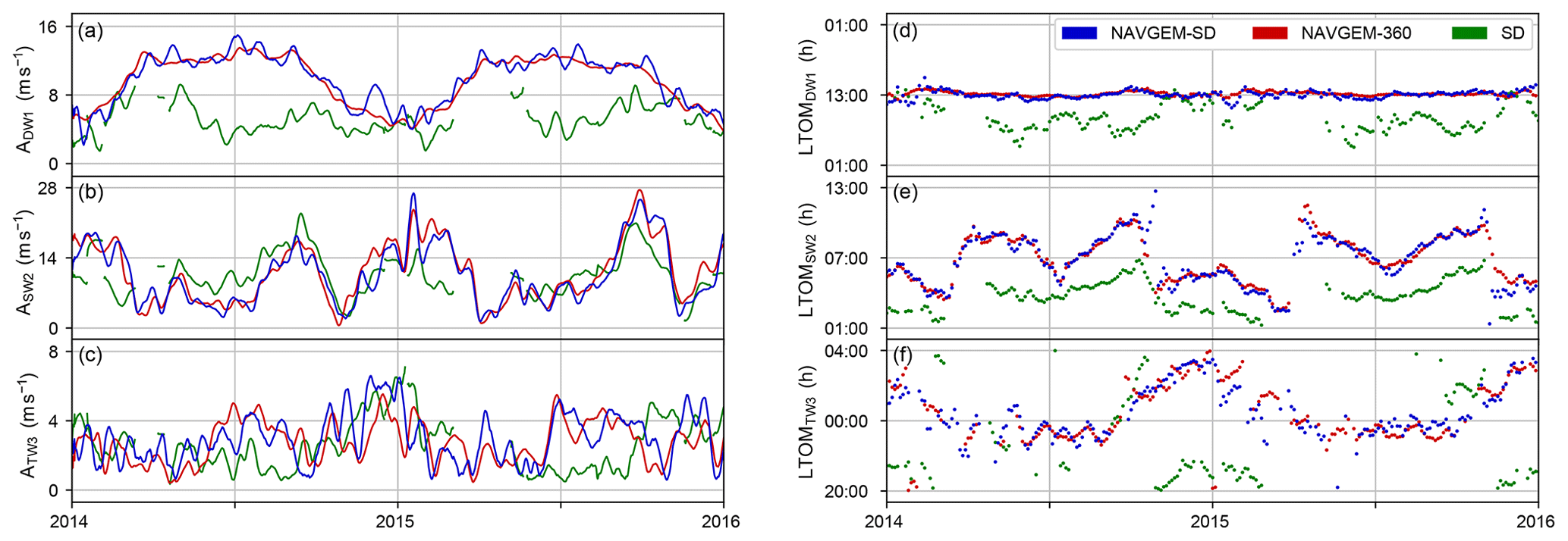
Figure 5Amplitude and phase of DW1 (a, d), SW2 (b, e), and TW3 (c, f) in NAVGEM-SD (blue) and NAVGEM-360 (red) meridional winds at 82.5 km altitude for the years 2014 and 2015. Phases are plotted as LTOM. Green curves show the corresponding meridional tides from around 95 km altitude as measured by the array of SuperDARN (SD) radars.
4.2 Root-mean-square error analysis
To examine the quality of the tides fitted to NAVGEM-SD, they are compared to those fitted to NAVGEM-360 by looking at the root-mean-square error (RMSE) between their respective tidal fields. Here the tidal fields themselves can be fully reconstructed on a 360∘ longitude–time grid using the three hourly fitted amplitudes and phases. To account for the changing availability of the SD stations with time, the RMSE is reported using 2014 NAVGEM-HA meridional winds sampled at the locations of active SD stations for each year between 2000 and 2016. The resulting year-by-year RMSE values, calculated between the yearly reconstructed tidal fields of NAVGEM-SD and NAVGEM-360, are shown in Fig. 6. For each year the RMSE is comparatively low relative to the absolute tidal amplitudes shown in Fig. 5, ensuring the validity of the method to extract the migrating tides over the range of hourly SD data used in this study. It also shows that the stations changing with time do not induce any substantial long-term trends.
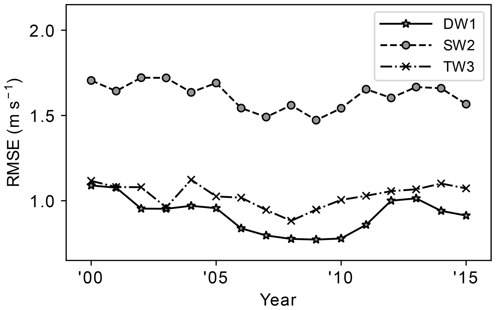
Figure 6Yearly RMSE between the tidal fields constructed from fits to NAVGEM-360 and NAVGEM-SD sampled at active SuperDARN stations for each year between 2000 and 2016.
In the above, sampling NAVGEM-360 at 60∘ N is motivated by NAVGEM-SD most closely corresponding to NAVGEM-360 at this latitude, which is now demonstrated. To that end, the RMSE is examined between NAVGEM-SD and NAVGEM-360, where the latter is taken at each latitude between 52 and 68∘ N. Figure 7 demonstrates that the RMSE for the SW2 and TW3 tidal fields reaches a clear minimum at 60∘ N, while the RMSE of DW1 decreases also for latitudes greater than 60∘ N. However, the relative difference between the RMSE of DW1 at 60 and 68∘ N is comparatively low (−2.4 %). The migrating tides extracted from NAVGEM-SD are therefore concluded to most closely correspond to those at 60∘ N. Following this conclusion, the migrating tides extracted from SD are taken to be most closely representative of those at 60∘ N.

Figure 7Yearly RMSE between the tidal fields constructed from fits to 2014 NAVGEM-SD and NAVGEM-360 taken along each latitude between 52 and 68∘ N.
The SW2 and TW3 tides isolated from 16 years of SD meteor winds show a well-defined and strongly recurring seasonal cycle. The main features of SW2, namely its amplitude peaks around early fall and mid-winter and sharp phase jumps around the equinoxes, are in qualitative agreement with previous observational and model studies of the mid- and high-latitude migrating semidiurnal tide (Wu et al., 2011; Xu et al., 2011; Forbes and Vial, 1989). The SW2 presented in this work indicates that the early fall amplitude peaks in the zonal and meridional winds are significantly higher than those in mid-winter, by 71 % and 56 % on average, respectively.
The seasonal cycle of TW3, showing a broad wintertime amplitude maximum and a near 4 h LTOM phase progression tracing a half-circle throughout winter, is also in qualitative agreement with previous (satellite) observational and model studies of the mid- and high-latitude migrating terdiurnal tide (Smith, 2000; Akmaev, 2001; Smith and Ortland, 2001). The pronounced amplitude peak around DOY 265 observed by SD uniquely stands out, however, possibly owing to the high temporal resolution offered by the radars. The DOY 265 amplitude peak appears to be an enhancement superimposed on the broad wintertime maximum. There are a number of mechanisms that can excite a time-localized forcing of TW3, such as non-linear wave–wave interactions and diurnal tide and gravity wave interactions (Teitelbaum et al., 1989; Miyahara and Forbes, 1991). Whether conditions are favorable for any such mechanisms to come into effect around DOY 265 remains to be examined. Here we note that a similar time-localized amplitude peak has been described in the zonal and meridional winds above 100 km altitude at 60∘ N in the Canadian Middle Atmosphere Model (CMAM) (Du and Ward, 2010). Further, we note that traditional single point radar measurements of the 8 h wave are prone to contamination by gravity waves, for which 8 h falls in the middle of the typical mid- to high-latitude spectrum at MLT heights (e.g., Conte et al., 2018). Gravity wave contamination is expected to be comparatively low for the TW3 tide retrieved from SD, however, since the horizontal scale of gravity waves is much smaller than the longitudinal extent covered by the radars.
The DW1 tide shows considerably more short-term and interannual variability and a different seasonal behavior between the zonal and meridional components. A possible cause of this is that DW1 has a relatively short vertical wavelength. Whereas the semidiurnal and terdiurnal tides have a vertical wavelength on the order of 100 km in the MLT (Chapman and Lindzen, 2012; Yuan et al., 2008; Smith, 2000), the diurnal tide has a vertical wavelength on the order of 25–35 km (e.g., Avery et al., 1989). The vertical wavelength of DW1 is therefore much nearer to the vertical average represented by the SD meteor winds, which can cause DW1 to partly cancel out over the meteor echo range. Nevertheless, the climatology of the meridional component of DW1 shows close agreement with the seasonal cycle of the diurnal (1,1) Hough mode calculated from TIMED Doppler Interferometer (TIDI) and NAVGEM-HA meridional winds by Dhadly et al. (2018). It is possible that certain diurnal modes are selectively filtered by SD based on their respective vertical wavelength and that the (1,1) mode is the dominant remaining mode, even though the amplitude of this mode broadly peaks around 25∘ N (Chapman and Lindzen, 2012). Future work could focus on investigating whether the climatology of the zonal component of DW1 in SD can also be associated with the diurnal (1,1) Hough mode.
This study has leveraged the longitudinal coverage of 10 high-latitude SuperDARN (SD) radars to isolate the DW1, SW2, and TW3 tides from 16 years of hourly meteor wind measurements of the mid- to high-latitude MLT. Based on sampling experiments with NAVGEM-HA, it is demonstrated that the SD tides are closely representative of the (global) migrating tides along 60∘ N. The amplitude and phase structure of SW2 and TW3 show a strongly recurring seasonal cycle, whereas DW1 shows considerably more year-to-year variability. Notable observations are that the climatological early fall amplitude maximum of SW2 in the zonal (meridional) wind is 8.3 (6.4) m s−1 greater than the mid-winter maximum and that TW3 is marked by a secondary amplitude peak around DOY 265 that reaches values of 5.3 ± 1.7 m s−1 in the zonal wind. In addition, DW1 is found to show a bi-modal circular phase polarization relation, where the zonal component leads the meridional during most of the year and vice versa during summer.
Many open questions remain in terms of how tidal variability is coupled to variability in their forcing mechanisms and propagation conditions. For future work, the time series of validated SD tidal measurements presented in this work can serve as a valuable source of data in studying the long- and short-term trends and variability of the migrating tides in the high-latitude MLT. The method and validation steps outlined in this work will also contribute to similar analyses of SD meteor winds from the continuously expanding global network of radars.
SuperDARN data are available from Virginia Tech at http://vt.superdarn.org/tiki-index.php, last access: 7 December 2020.
WEC, PJE and REH developed the concept, while WEC performed the data analysis and wrote the paper. JPM provided NAVGEM-HA data and contributed to Sect. 2.3. PJE, REH and JPM gave feedback on the development of this work.
The authors declare that they have no conflict of interest.
The authors acknowledge the use of the SuperDARN meteor wind data product. The SuperDARN project is funded by national scientific funding agencies of Australia, China, Canada, France, Japan, Italy, Norway, South Africa, the United Kingdom, and the United States. Development of NAVGEM-HA was supported by the Chief of Naval Research and the Department of Defense High Performance Computing Modernization Project. The authors thank two anonymous reviewers for their assistance in improving this work.
This research has been supported by the Research Council of Norway (grant no. 223525/F50).
This paper was edited by Dalia Buresova and reviewed by two anonymous referees.
Akmaev, R. A.: Seasonal variations of the terdiurnal tide in the mesosphere and lower thermosphere: A model study, Geophys. Res. Lett., 28, 3817–3820, https://doi.org/10.1029/2001gl013002, 2001. a
Arnold, N. F., Cook, P. A., Robinson, T. R., Lester, M., Chapman, P. J., and Mitchell, N.: Comparison of D-region Doppler drift winds measured by the SuperDARN Finland HF radar over an annual cycle using the Kiruna VHF meteor radar, Ann. Geophys., 21, 2073–2082, https://doi.org/10.5194/angeo-21-2073-2003, 2003. a
Avery, S., Vincent, R., Phillips, A., Manson, A., and Fraser, G.: High-latitude tidal behavior in the mesosphere and lower thermosphere, J. Atmos. Sol.-Terr. Phy., 51, 595–608, https://doi.org/10.1016/0021-9169(89)90057-3, 1989. a
Chapman, S. and Lindzen, R. S.: Atmospheric tides: thermal and gravitational, Springer Science & Business Media, 179 pp., 2012. a, b, c
Chisham, G.: Calibrating SuperDARN Interferometers Using Meteor Backscatter, Radio Sci., 53, 761–774, https://doi.org/10.1029/2017rs006492, 2018. a
Chisham, G. and Freeman, M. P.: A reassessment of SuperDARN meteor echoes from the upper mesosphere and lower thermosphere, J. Atmos. Sol.-Terr. Phy., 102, 207–221, https://doi.org/10.1016/j.jastp.2013.05.018, 2013. a, b
Conte, J. F., Chau, J. L., Laskar, F. I., Stober, G., Schmidt, H., and Brown, P.: Semidiurnal solar tide differences between fall and spring transition times in the Northern Hemisphere, Ann. Geophys., 36, 999–1008, https://doi.org/10.5194/angeo-36-999-2018, 2018. a
Dhadly, M. S., Emmert, J. T., Drob, D. P., McCormack, J. P., and Niciejewski, R. J.: Short-Term and Interannual Variations of Migrating Diurnal and Semidiurnal Tides in the Mesosphere and Lower Thermosphere, J. Geophys. Res., 123, 7106–7123, https://doi.org/10.1029/2018ja025748, 2018. a, b
Du, J. and Ward, W. E.: Terdiurnal tide in the extended Canadian Middle Atmospheric Model (CMAM), J. Geophys. Res.-Atmos., 115, D24106, https://doi.org/10.1029/2010jd014479, 2010. a
Eckermann, S. D., Ma, J., Hoppel, K. W., Kuhl, D. D., Allen, D. R., Doyle, J. A., Viner, K. C., Ruston, B. C., Baker, N. L., Swadley, S. D., Whitcomb, T. R., Reynolds, C. A., Xu, L., Kaifler, N., Kaifler, B., Reid, I. M., Murphy, D. J., and Love, P. T.: High-Altitude (0-100 km) Global Atmospheric Reanalysis System: Description and Application to the 2014 Austral Winter of the Deep Propagating Gravity Wave Experiment (DEEPWAVE), Mon. Weather Rev., 146, 2639–2666, https://doi.org/10.1175/mwr-d-17-0386.1, 2018. a
Fisher, N. I.: Statistical analysis of circular data, cambridge university press, 257 pp., 1995. a
Forbes, J. and Vial, F.: Monthly simulations of the solar semidiurnal tide in the mesosphere and lower thermosphere, J. Atmos. Sol.-Terr. Phy., 51, 649–661, https://doi.org/10.1016/0021-9169(89)90063-9, 1989. a
Garcia, R. R., Lieberman, R., Russell, J. M., and Mlynczak, M. G.: Large-Scale Waves in the Mesosphere and Lower Thermosphere Observed by SABER, J. Atmos. Sci., 62, 4384–4399, https://doi.org/10.1175/jas3612.1, 2005. a
Hall, G. E., MacDougall, J. W., Moorcroft, D. R., St.-Maurice, J.-P., Manson, A. H., and Meek, C. E.: Super Dual Auroral Radar Network observations of meteor echoes, J. Geophys. Res., 102, 14603–14614, https://doi.org/10.1029/97ja00517, 1997. a, b
Hibbins, R. E. and Jarvis, M. J.: A long-term comparison of wind and tide measurements in the upper mesosphere recorded with an imaging Doppler interferometer and SuperDARN radar at Halley, Antarctica, Atmos. Chem. Phys., 8, 1367–1376, https://doi.org/10.5194/acp-8-1367-2008, 2008. a
Hibbins, R. E., Espy, P. J., Orsolini, Y. J., Limpasuvan, V., and Barnes, R. J.: SuperDARN Observations of Semidiurnal Tidal Variability in the MLT and the Response to Sudden Stratospheric Warming Events, J. Geophys. Res.-Atmos., 124, 4862–4872, https://doi.org/10.1029/2018jd030157, 2019. a
Laskar, F. I., McCormack, J. P., Chau, J. L., Pallamraju, D., Hoffmann, P., and Singh, R. P.: Interhemispheric Meridional Circulation During Sudden Stratospheric Warming, J. Geophys. Res., 124, 7112–7122, https://doi.org/10.1029/2018ja026424, 2019. a
McCormack, J., Hoppel, K., Kuhl, D., de Wit, R., Stober, G., Espy, P., Baker, N., Brown, P., Fritts, D., Jacobi, C., Janches, D., Mitchell, N., Ruston, B., Swadley, S., Viner, K., Whitcomb, T., and Hibbins, R.: Comparison of mesospheric winds from a high-altitude meteorological analysis system and meteor radar observations during the boreal winters of 2009-2010 and 2012-2013, J. Atmos. Sol.-Terr. Phy., 154, 132–166, https://doi.org/10.1016/j.jastp.2016.12.007, 2017. a, b
Miyahara, S. and Forbes, J. M.: Interactions between Gravity Waves and the Diurnal Tide in the Mesosphere and Lower Thermosphere, J. Meteorol. Soc. Jpn., 69, 523–531, https://doi.org/10.2151/jmsj1965.69.5_523, 1991. a
Ortland, D. A.: Daily estimates of the migrating tide and zonal mean temperature in the mesosphere and lower thermosphere derived from SABER data, J. Geophys. Res.-Atmos., 122, 3754–3785, https://doi.org/10.1002/2016jd025573, 2017. a
Pancheva, D. and Mukhtarov, P.: Atmospheric Tides and Planetary Waves: Recent Progress Based on SABER/TIMED Temperature Measurements (2002-2007), in: Aeronomy of the Earth's Atmosphere and Ionosphere, Springer Netherlands, 19–56, https://doi.org/10.1007/978-94-007-0326-1_2, 2011. a
Reid, I. M.: MF and HF radar techniques for investigating the dynamics and structure of the 50 to 110 km height region: a review, Progress in Earth and Planetary Science, 2, 33, https://doi.org/10.1186/s40645-015-0060-7, 2015. a
Sakazaki, T., Fujiwara, M., and Shiotani, M.: Representation of solar tides in the stratosphere and lower mesosphere in state-of-the-art reanalyses and in satellite observations, Atmos. Chem. Phys., 18, 1437–1456, https://doi.org/10.5194/acp-18-1437-2018, 2018. a
Salby, M. L.: Sampling Theory for Asynoptic Satellite Observations, Part I: Space-Time Spectra, Resolution, and Aliasing, J. Atmos. Sci., 39, 2577–2600, https://doi.org/10.1175/1520-0469(1982)039<2577:STFASO>2.0.CO;2, 1982. a
Smith, A. K.: Structure of the terdiurnal tide at 95 km, Geophys. Res. Lett., 27, 177–180, https://doi.org/10.1029/1999gl010843, 2000. a, b
Smith, A. K.: Global Dynamics of the MLT, Surv. Geophys., 33, 1177–1230, https://doi.org/10.1007/s10712-012-9196-9, 2012. a
Smith, A. K. and Ortland, D. A.: Modeling and Analysis of the Structure and Generation of the Terdiurnal Tide, J. Atmos. Sci., 58, 3116–3134, https://doi.org/10.1175/1520-0469(2001)058<3116:MAAOTS>2.0.CO;2, 2001. a
Stober, G., Baumgarten, K., McCormack, J. P., Brown, P., and Czarnecki, J.: Comparative study between ground-based observations and NAVGEM-HA analysis data in the mesosphere and lower thermosphere region, Atmos. Chem. Phys., 20, 11979–12010, https://doi.org/10.5194/acp-20-11979-2020, 2020. a
Teitelbaum, H., Vial, F., Manson, A., Giraldez, R., and Massebeuf, M.: Non-linear interaction between the diurnal and semidiurnal tides: terdiurnal and diurnal secondary waves, J. Atmos. Terr. Phy., 51, 627–634, https://doi.org/10.1016/0021-9169(89)90061-5, 1989. a
Wu, Q., Ortland, D., Solomon, S., Skinner, W., and Niciejewski, R.: Global distribution, seasonal, and inter-annual variations of mesospheric semidiurnal tide observed by TIMED TIDI, J. Atmos. Sol.-Terr. Phy., 73, 2482–2502, https://doi.org/10.1016/j.jastp.2011.08.007, 2011. a
Xu, X., Manson, A. H., Meek, C. E., Jacobi, C., Hall, C. M., and Drummond, J. R.: Mesospheric wind semidiurnal tides within the Canadian Middle Atmosphere Model Data Assimilation System, J. Geophys. Res., 116, D17102, https://doi.org/10.1029/2011jd015966, 2011. a
Yuan, T., Schmidt, H., She, C. Y., Krueger, D. A., and Reising, S.: Seasonal variations of semidiurnal tidal perturbations in mesopause region temperature and zonal and meridional winds above Fort Collins, Colorado (40.6∘ N, 105.1∘ W), J. Geophys. Res., 113, D20103, https://doi.org/10.1029/2007jd009687, 2008. a