Measuring diameters and velocities of artificial raindrops with a neuromorphic event camera

Micev, Kire; Steiner, Jan; Aydin, Asude; Rieckermann, Jörg; Delbruck, Tobi

doi:https://doi.org/10.5194/amt-17-335-2024

Articles | Volume 17, issue 1

https://doi.org/10.5194/amt-17-335-2024

Articles | Volume 17, issue 1

Research article

18 Jan 2024

Research article |

| 18 Jan 2024

Measuring diameters and velocities of artificial raindrops with a neuromorphic event camera

Kire Micev, Jan Steiner, Asude Aydin, Jörg Rieckermann, and Tobi Delbruck

Video abstract

Abstract

Hydrometers that measure size and velocity distributions of precipitation are needed for research and corrections of rainfall estimates from weather radars and microwave links. Existing optical disdrometers measure droplet size distributions, but underestimate small raindrops and are impractical for widespread always-on IoT deployment. We study the feasibility of measuring droplet size and velocity using a neuromorphic event camera. These dynamic vision sensors asynchronously output a sparse stream of pixel brightness changes. Droplets falling through the plane of focus of a steeply down-looking camera create events generated by the motion of the droplet across the field of view. Droplet size and speed are inferred from the hourglass-shaped stream of events. Using an improved hard disk arm actuator to reliably generate artificial raindrops with a range of small sizes, our experiments show maximum errors of 7 % (mean absolute percentage error) for droplet sizes from 0.3 to 2.5 mm and speeds from 1.3 to 8.0 m s⁻¹. Measurements with the same setup from a commercial PARSIVEL disdrometer show similar results. Both devices slightly overestimate the small droplet volume with a volume overestimation of 25 % from the event camera measurements and 50 % from the PARSIVEL instrument. Each droplet requires processing of 5000 to 50 000 brightness change events, potentially enabling low-power always-on disdrometers that consume power proportional to the rainfall rate. Data and code are available at the paper website https://sites.google.com/view/dvs-disdrometer/home (Micev et al., 2023).

Download & links

Article (PDF, 9444 KB)

Download & links

How to cite.

Received: 09 Feb 2023 – Discussion started: 17 Apr 2023 – Revised: 22 Sep 2023 – Accepted: 31 Oct 2023 – Published: 18 Jan 2024

1 Introduction

There are increasing numbers of optical disdrometers that measure the diameter and speed of hydrometeors at ground level (Liu et al., 2013; Johannsen et al., 2020; Löffler-Mang and Joss, 2000; Bailey, 2016; Singh et al., 2021; Rees et al., 2021). Their drop size distribution (DSD) measurements are useful for predicting soil erosion and can be combined with weather radars or microwave links to predict a DSD over a larger area (Kruger and Krajewski, 2002; Špačková et al., 2021). Laser disdrometers are commonly installed at airports and wind farms for automated assessment of ground-level precipitation. Optical disdrometers measure the size and speed of hydrometeors either by direct observation or by occlusion of laser sheets, making them potentially easier to calibrate and maintain in the field than popular acoustic (Joss and Waldvogel, 1967, 1977; Distromet Ltd., 2022) and innovative evaporation-based disdrometers (Singh et al., 2021). The State of the Art (SoA) scientific video disdrometer is the two-dimensional video disdrometer (2DVD) first described by Kruger and Krajewski (2002)¹. However, 2DVD and competing particle size velocity (PARSIVEL) laser-sheet disdrometers have been reported to underestimate total rainfall volume and drift over time, resulting in impractical long-term deployment (Johannsen et al., 2020; Jaffrain and Berne, 2011; Upton and Brawn, 2008). Different types of disdrometers have been shown to produce measured DSDs that differ dramatically for small droplets (Johannsen et al., 2020; Cao et al., 2008). They consume significant static power, making it difficult to deploy them in solar-powered weather monitoring, where brownouts can occur in dark weather conditions (Špačková et al., 2021). An event camera disdrometer could provide a field device that would have simple optical and lighting requirements and would be accurate over a wide range of precipitation sizes to enable autonomous continuous DSD measurements that use less power when there are fewer droplets to measure.

This paper studies the feasibility of using a novel droplet-driven sampling approach based on analyzing the brightness change events produced by a dynamic vision sensor (DVS) event camera. Such an event camera does not capture stroboscopic images using a shutter like a conventional camera. Instead, each pixel reports asynchronous changes in brightness as they occur, and stays silent otherwise (Fig. 1a, Sect. 2.2) (Lichtsteiner et al., 2008; Gallego et al., 2020). They have been successfully used in many high speed robotics and machine vision applications (Gallego et al., 2020), but not yet in environmental or atmospheric monitoring.

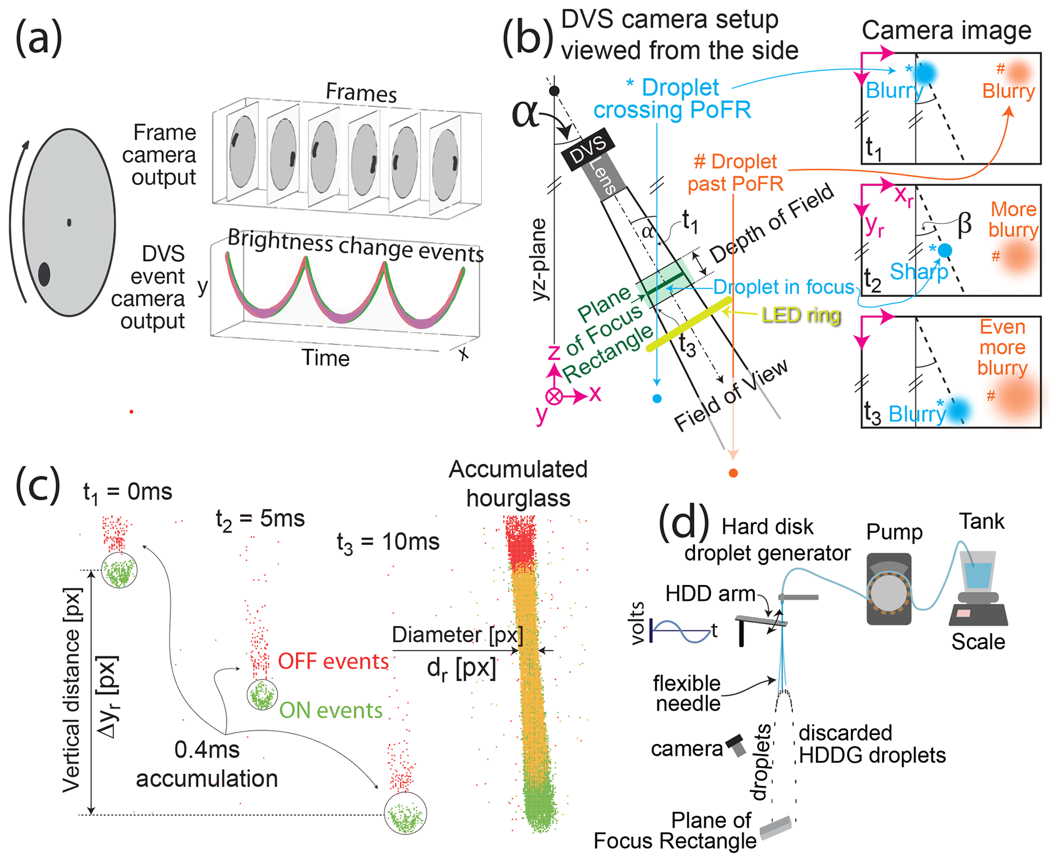
https://amt.copernicus.org/articles/17/335/2024/amt-17-335-2024-f01

Figure 1Summary of dynamic vision sensor disdrometer (DVSD) methods. (a) Comparison between a conventional frame camera and a DVS capturing a rotating disk with a black dot. The frame camera outputs frames with finite exposure duration at discrete time intervals, whereas the event camera continuously outputs brightness change events, which results in a helix of discrete events in the space time plot (green: increase in brightness, red: decrease in brightness) (Lichtsteiner et al., 2008; Gallego et al., 2020) (Sect. 2.2). (b) Side view of the DVS camera setup in experiments and three illustrations of DVS recordings. The cyan droplet (^*) crosses the field of view (FoV) and falls through the plane of focus rectangle (PoFR), which is tilted at a small angle α from the vertical yz plane. The corresponding camera image is illustrated on the right side at three different times: the cyan droplet (^*) enters the FoV; it starts out blurry, comes into focus, and then grows blurry again as it exits the FoV. By contrast, the orange droplet (#) crosses the FoV behind the PoFR; it never comes into focus and only grows increasingly blurry. β is the angle of the droplet from the vertical y_r axis seen on the recording, caused by droplet velocity component in the yz plane (out of the page). (c) Sample DVS recording of a droplet crossing the PoFR, which is demonstrated in three frames with 5 ms time differences between each frame. Each of the three DVS frames in this sample is an accumulation of 0.4 ms of events. Green points correspond to ON events, red points show OFF, and yellow points show overlapping of ON and OFF events. The rightmost frame shows all accumulated events over 10 ms. Each droplet creates 10k to 50k events, depending on its size. The diameter d_r of the droplet is measured at the waist of the hourglass when the droplet is in focus, as illustrated on the right. We estimate the falling speed v_r by measuring the focal plane speed of the droplet. Equations (1) and (2) provide the physical droplet diameter and speed. (Sect. 2.5.3) (d) Hard disk droplet generator (HDDG) modified from Kosch and Ashgriz (2015). The droplet generator uses a hard disk actuator to oscillate a flexible needle with a constant flow rate of water fed into the needle from a pump. The water tank is placed on top of a scale to calculate the flow rate. Within a 4× range of oscillation frequencies, a droplet is released at each end of the oscillation by large acceleration forces acting on the flexible needle. The diameter of droplets released from the needle is adjusted by the oscillation frequency of the needle. We generated the large 2.5 mm droplets falling 10 m through a circular staircase well with an intravenous (IV) dripper.

Our main contributions are:

1.
We propose a novel optical disdrometer method that exploits the activity-driven output and high time resolution of DVS brightness change events to efficiently measure individual droplet size and speed using the shallow depth of field of a fast lens to localize individual droplets in a 3D space.
2.
We generate high-quality ground truth data for small droplets by modifying the HDDG from Kosch and Ashgriz (2015) and report how to reproduce it.
3.
We report the first measurements of droplet size and speed with our proposed method and show that the DSD satisfactorily aligns with the ground truth data with at most a mean absolute percentage error of 7 %. We show that our method measures small droplets with equivalent precision and smaller bias than a commercial PARSIVEL disdrometer.

2 Materials and methods

2.1 Overview of the Dynamic Vision Sensor Disdrometer (DVSD) method

Figure 1 provides an overview of our proposed DVSD method, which is detailed in later sections. The DVS camera (Fig. 1a, Sect. 2.2) asynchronously reports brightness change events as the droplets pass through a thin depth of field (DoF) at the PoFR from a lens that looks down on the rainfall from a steep angle (Fig. 1b). The droplets are illuminated from behind with a ring of LEDs to produce bright droplet edges (Appendix F). Each droplet produces about 10 000 DVS brightness change events (Fig. 1c). By a simple analysis of this spatiotemporal cluster of events, the DVSD method can measure both the size and the speed of the droplet (Sect. 2.5.3). We developed a modified HDDG to generate small droplets (Fig. 1d, Sect. 2.3.2) and used an intravenous dripper droplet generator (IVDG) for large droplets (Sect. 2.3.1). Figure 1c shows an illuminated falling water droplet recorded with the DVS camera. Our method consists of two key principles. First, we aim the camera downward at a steep angle, with an angle α from the vertical (Fig. 1b: left). Second, the diameters of the droplets crossing the shallow DoF at the plane of focus (PoF) are measured unambiguously, i.e., because the PoF is located at a fixed working distance from the lens, we can infer the 3D position of the droplet, and hence disambiguate the absolute size from the image size. Droplets passing through the camera's PoFR come into focus, showing a high contrast and creating an hourglass-shaped cluster of events, whereas droplets outside the PoFR do not come into focus or create an hourglass cluster. Droplet velocity is measured by using short accumulation time at two points in time (Fig. 1c, Sect. 2.5.3). Accumulating the events belonging to one droplet that crosses the PoFR (marked by ^* in figure) produces an hourglass shape (Fig. 1c: accumulated hourglass) where the ideal moment for a droplet diameter measurement (Sect. 2.5.3) is at the waist of this hourglass. The hourglass should be as concave as possible to facilitate the detection of the waist. Using a fast lens with a small aperture ratio f number produces a shallow DoF, increasing the amount of blur of the droplets that are out of focus. Figure 1b also illustrates how a droplet that crosses the FoV but past the PoFR (marked by # in figure) creates an accumulated image that starts out blurry and becomes increasingly blurry until it leaves the FoV; similarly (but not illustrated), a droplet that crosses the FoV in front of the PoFR creates an accumulated event image that starts out blurry and becomes increasingly sharper until it leaves the FoV. Only droplets that cross the PoFR create hourglasses.

2.2 Dynamic vision sensor event camera

The DVSD uses a DVS event camera (Lichtsteiner et al., 2008), specifically a DAVIS346² (Taverni et al., 2018). In each pixel (Fig. 2), the logarithmic photoreceptor (A) drives a change detector (B) that generates the ON and OFF events (D). Pixel photoreceptors continuously transduce the photocurrent I produced by the photodiode (PD) to a logarithmic voltage V_p, resulting in a dynamic range of more than 120 dB. This logarithmic voltage (called brightness here) is buffered by a unity-gain source follower to the voltage V_sf, which is stored in a capacitor C_DVS inside individual pixels, where it is continuously compared with the new input. If the change V_d in log intensity exceeds a critical event threshold, an ON or OFF event is generated, representing an increase or decrease in brightness. The event thresholds θ_on and θ_off are nominally identical for the entire array. The time interval between individual events is inversely proportional to the derivative of the brightness. When an event is generated, the pixel's location and the sign of the brightness change are immediately transmitted to an arbiter circuit surrounding the pixel array, then off-chip as a pixel address, and a timestamp is assigned to individual events. The arbiter circuit then resets the pixel's change detector so that the pixel can generate a new event. Events can be read out at up to rates of about 10 MHz. The quiescent (noise) event rate is a few kHz. Events are transmitted from the DAVIS chip to a host computer over a universal serial bus (USB). The host software records the data and allows playback in slow motion. In addition to the DVS circuit the DAVIS346 also has a circuit for conventional intensity frame recordings called the active pixel sensor (APS) circuit (Fig. 2c), which was useful for lens calibration and focusing.

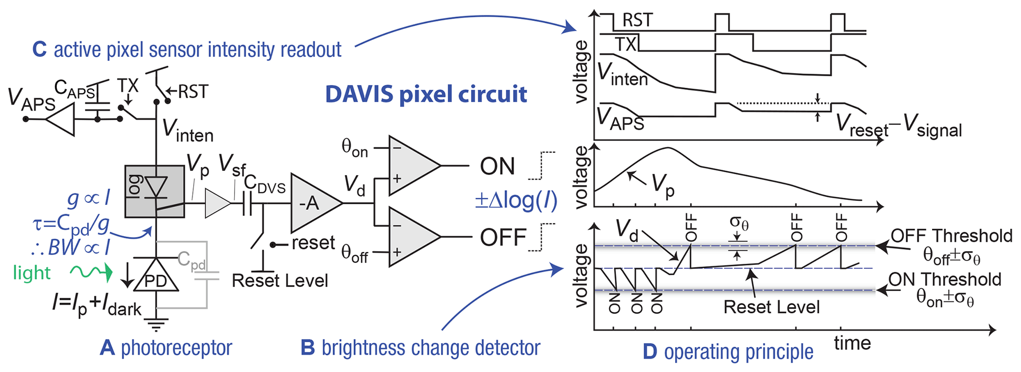
https://amt.copernicus.org/articles/17/335/2024/amt-17-335-2024-f02

Figure 2DAVIS pixel circuit and operating principle. The sensor generates asynchronous brightness change ON and OFF DVS events and APS intensity samples, which we do not use for disdrometry but which are helpful for calibration and focusing. Asynchronous digital circuits place the event $(x, y, p)$ address (p is the event polarity) onto a shared digital output bus. A USB chip on the camera transmits these events to a host computer along with the event timestamps t. The computer supplies packets of these $(t, x, y, p)$ events with a maximum latency of 1 ms to user programs.

Download

2.3 Artificial droplet creation

Figures 1d, 3, and B1 illustrate our HDDG for creating small droplets. It is based on previous work by Kosch and Ashgriz (2015), who utilized a computer hard disk arm as an actuator. They used a high-frequency buzz to create ripples in a steady stream of water emitted by a stiff glass needle, which would break up into small droplets. Our HDDG uses a flexible plastic needle, which, if properly combined with a steady stream of water, creates a single droplet at each end of an oscillation, resulting in two droplet streams, one of which we measured. We used a discarded hard disk drive that we disassembled to expose the platter head actuator arm. The arm is coupled to the needle by threading the needle through adhesive tape applied over the hole in the arm, allowing the needle to protrude. The arm is actuated with a home audio power amplifier driven by sinusoidal waveforms generated by an audio wave generating program where we used coil driver amplitudes from 5 to 20 V peak-to-peak and frequencies from 60 to 220 Hz.

2.3.1 Intravenous droplet generator

Figures B2 and 4b shows our setup for creating large droplets with an intravenous dripper droplet generator (IVDG) assembled from a standard intravenous dripper obtained from a pharmacy and a needle tip intended for glue dispensers³. The diameter of the needle tip (OD 0.4 mm) has only a weak influence on the droplet size (≈ 2.5 mm), which is mainly determined by the surface tension of water adhering to the needle; at low flow rates, when the droplet mass grows large enough, it breaks free from the needle. We adjusted the IV flow to produce a regular series of droplets at a rate of about 1.6 Hz (Appendix E).

2.3.2 Hard disk droplet generator

Figure 1d illustrates our HDDG and Figs. B1 and 4 show the HDDG setup. Our HDDG is based on previous work by Kosch and Ashgriz (2015), who utilized a computer hard disk arm as an actuator. They used a high-frequency buzz to create ripples in a steady stream of water emitted by a stiff glass needle, which would break up into small droplets with a diameter of about 100 µm. Our HDDG uses a soft and flexible plastic needle, which, if properly combined with a controlled stream of water, reliably creates a single droplet at each end of an oscillation, resulting in two droplet streams, one of which we measured.

HDDG droplet needle. To make the droplet needle, we use a microloader microcapillary tip⁴ This soft plastic needle tubing protrudes from its integrated feeder expansion. The peristaltic pump tubing⁵ is plugged into this microloader. The needle is threaded through a hole drilled through the HDD actuator arm so that the needle protrudes from the arm by 2 to 4 cm, and we can control the length of the protruding needle to adjust its resonance frequency to match the driving frequency. In that way, we can use a lower driving voltage and current for the HDD driver coils. The needle is fixed to an elevated platform with a conical interference fit between the needle and a black plastic tube glued to that platform (see Fig. B1c and d).

Construction of HDDG droplet generator. Figure 3 sketches the HDDG construction. We use an old 250 GB 3.5^′′ hard disk drive that we disassembled to expose the platter head actuator arm. The coil driver wires have two functions: first, to power the HDD coils and second, to act like springs to keep the HDD arm close to the middle of the two permanent magnets, which is the best operating point for the arm. To construct the needle driver, we follow these steps:

1.
The upper end of the plastic needle is frictionally held in place (see black tube).
2.
Two nuts and a bolt (Fig. B1d) adjust the protruding length of the needle to match the resonance frequency of the needle with the HDD frequency to maximize the amplitude of the oscillation and, therefore, the efficiency.
3.
The lower end of the plastic needle is guided through a tiny hole in a piece of sticky tape. The tape is attached to the end of the HDD arm.
4.
The needle is connected to the water tube from the pump. This connection must be tight to prevent water leakage and to prevent the needle from twisting.
5.
As the needle has some inherent curvature, we twisted it with our fingers until the inherent curvature was perpendicular to the oscillation direction.

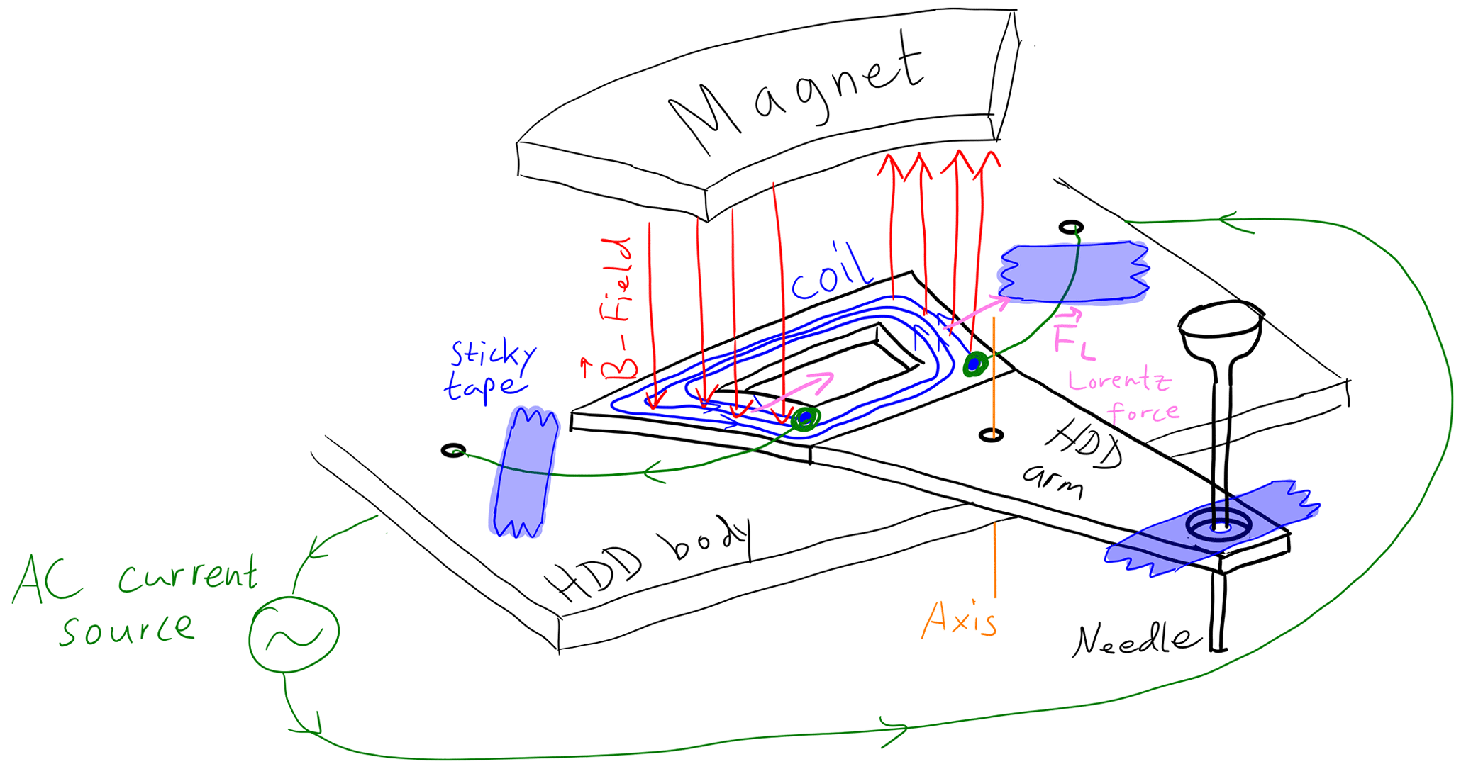
https://amt.copernicus.org/articles/17/335/2024/amt-17-335-2024-f03

Figure 3Sketch of HDDG. The red B-vector is the induced magnetic field by the coil and alternates its direction from up to down. When it points up, it is attracted to upwards pointing yellow B-vectors from the static magnet. Two sticky tapes and two green wires hold the HDD arm in place in a spring-like manner. This attachment ensures that the coil is centered between the two opposite poles of the metal piece. Without the sticky tapes, we observed that the arm drifts to one side and no longer functions properly. See Fig. B1 for photos.

Download

Driving the HDD. The HDD arm is actuated with an audio power amplifier driven by sinusoidal waveforms generated by an audio wave generating program (https://www.szynalski.com/tone-generator/, last access: 20 December 2023). The arm is coupled to the needle by threading the needle through one-sided adhesive tape, which is applied over the hole in the arm. We used amplitudes from 3 to 10 Vpp and frequencies from 60 to 220 Hz. By adjusting the flow rate and oscillation frequency, we can arrive at a combination of settings where in nearly every oscillation, a single droplet is flung from the needle tip at each end of the oscillation. As the flow rate and frequency are constant, the droplet sizes are also constant.

2.4 Experimental setups for DVSD and PARSIVEL measurements

Figure 4 illustrate the HDDG and IVDG setups. Figures. B1 and B2 show detailed photos of the setups.

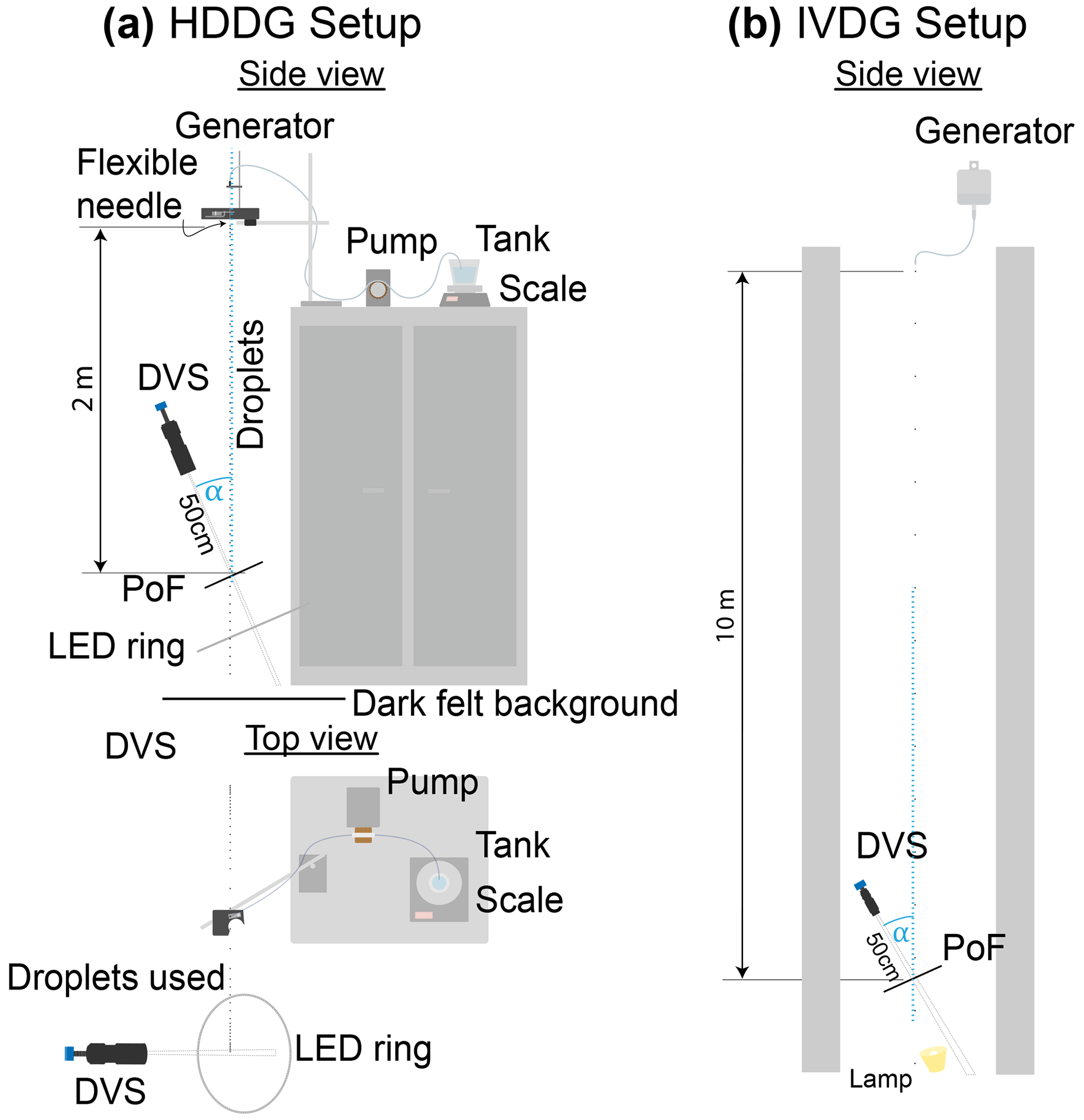
https://amt.copernicus.org/articles/17/335/2024/amt-17-335-2024-f04

Figure 4Illustration of experimental setups. (a) HDDG setup is illustrated from a side view and a from a top view perspective. (b) IVDG setup is illustrated from a side view perspective.

Download

We replicated both sets of experiments with the commercial PARSIVEL instrument listed in Table 4. For the PARSIVEL IVDG experiment, we used a different stairwell that is much more open to wind currents because the circular one used for the DVSD experiments was not available.

For the DVS measurements we optimized the camera biases for droplet observation by increasing the pixel bandwidth and optimizing the event threshold settings. The DVS are recorded on disk as AEDAT-2.0 files using jAER (https://jaerproject.net, last access: 20 December 2023).

For the PARSIVEL measurements, we used the default device settings. The PARSIVEL records the droplet class counts and writes them to summary CSV files.

2.5 Experiments

The objective of the experiments was to measure the diameter and velocity of droplets with a DVS with droplets falling close to their terminal speed, and to compare these measurements with their corresponding ground truth (GT) (Sect. 2.5.4), and to PARSIVEL measurements using the same setups (Sect. 3.2). Two experiments were conducted with different setups to optimize droplet creation for two different drop size categories, which are further explained in the following two paragraphs. Both experiments used the same DVS camera and measurement principles (described in Sect. 2.5.3). Lenses for each experiment were chosen to make the droplets create a diameter of at least 10 px at the PoF. Both lenses were set at their minimum focusing distance. The working distance was then reduced further to about 50 cm using lens spacers.

Table 1 compares the two experimental setups with further details. Both droplet generation methods are described in Sect. 2.3.

Table 1Detailed setup parameters for the HDDG and IVDG experiments. See also Table G1.

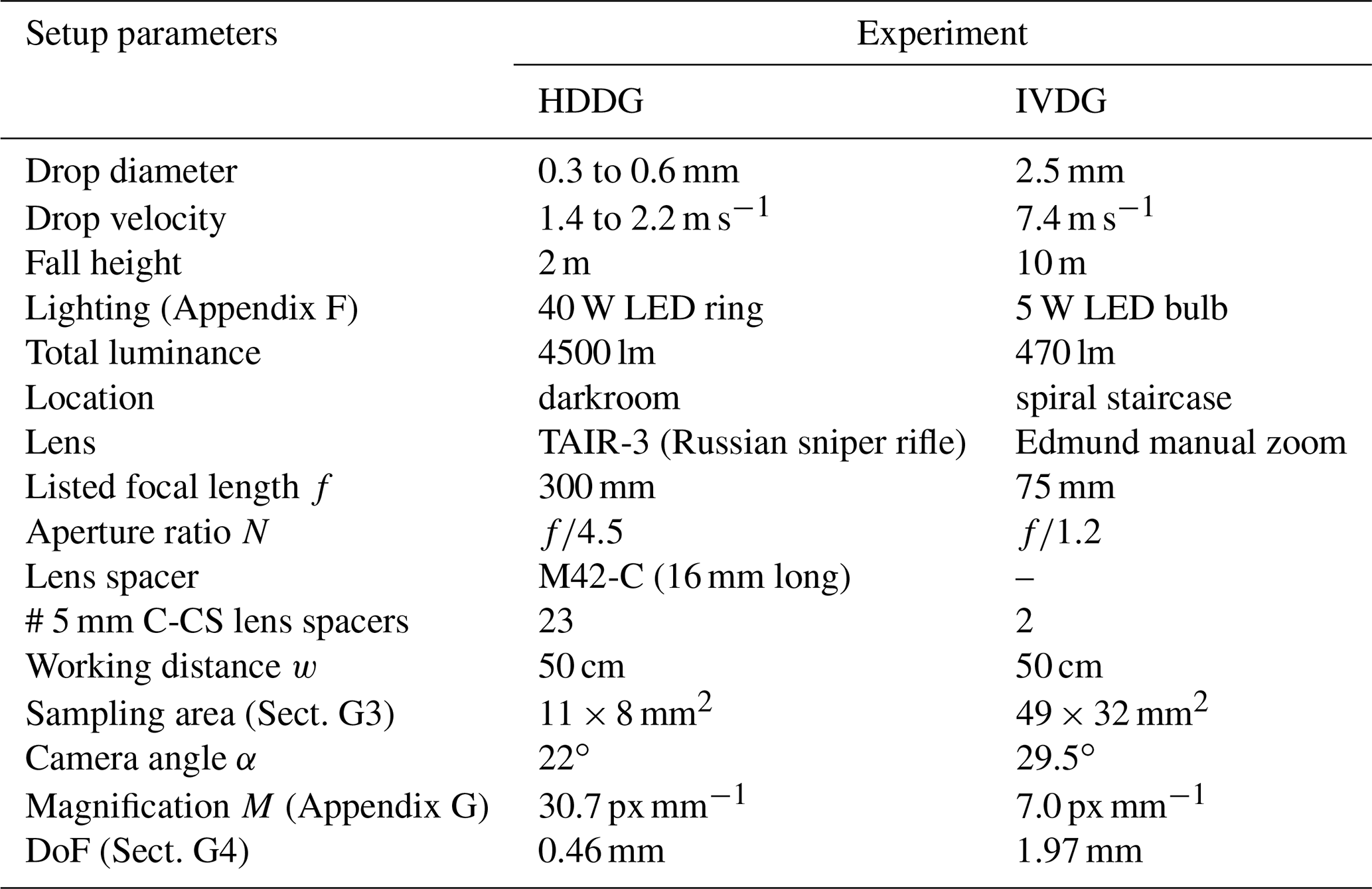
Download Print Version | Download XLSX

The first experiments, called HDDG experiments, were conducted in a darkroom using an HDDG and a fall height of 2 m. This setup was optimized for droplets with a diameter of 0.3 to 0.6 mm, by using a 300 mm lens with the resulting large magnification M=30.7 px mm⁻¹. This led to a sampling area of 0.9 cm². The HDDG produced a localized drop jet, making it fairly easy to hit the sampling area. The height of the droplet fall is enough for the drops to reach more than 99 % of the terminal velocity according to Appendix H. We used a 40 W Light Emitting Diode (LED) ring purchased from a home supply store as a light source pointing upward and inward to achieve a high contrast between the bright drop edges and the dark background (Fig. B1a and Appendix F).

The second experiment, called the IVDG experiment, was carried out in the vertical tunnel of a spiral staircase using a IVDG as a droplet generator and a fall height of more than 10 m. With a smaller magnification of 7 px mm⁻¹ (4.4× smaller than for the HDDG experiments), the magnification was reduced for droplets with a diameter of approximately 2.5 mm, while maintaining a relative precision similar to that of the HDDG setup. The main reason for this reduction in magnification was to capture the droplets, which had a huge scatter compared with the HDDG scatter, more easily. With the IVDG, it was only possible to create a single droplet size because the droplet size is determined by the weight that breaks the surface tension with the needle. The higher magnification led to a larger sampling area of 4 cm², increasing the chance of capturing the larger drops, which have a much greater spread from the higher fall needed to achieve a final speed close to the terminal speed. The height of the fall is sufficient for the drops to reach more than 97 % of the terminal velocity according to Appendix H. The working space of the experiment IVDG was more limited (Fig. B2b), so we used a single 5 W LED reading lamp to illuminate the drops from behind, which refracted the light toward the middle of the drop, leaving the edges dark. Despite this non-optimal lighting, we could still determine the width and velocity of the droplets from the recordings.

A key factor was the adjustable angle of the camera from the vertical α (see Fig. 1b: left). The smaller the α, the more accurately the diameter can be measured and the larger the horizontal sampling area, which leads to a faster estimate of DSD. Larger αs allow more precise velocity measurements but a smaller sampling area. The sampling area is the total area of the PoF inside the FoV multiplied by cos α. According to our findings, 20 to 30^∘ was optimal for α.

Equation (1) of Sect. 2.5.3 was used for the diameter calculation. To compute the velocity, we used the nonsimplified formula on the left side of Eq. (2) for the HDDG experiment, and used the simplified formula on the right side of Eq. (2) for the IVDG experiment owing to the negligible horizontal velocity component on the recording (see Fig. 1b: right). Appendix G describes how we measured the parameters.

2.5.1 Data selection

Each recording session collected data for a single droplet size. From the recording, we manually selected droplets that crossed the image and created a distinct hourglass shape. These droplets cross the PoFR sampling area and thus allow a reliable DSD to be inferred. Figure 1 illustrated how this procedure excluded droplets that did not pass through the PoF.

2.5.2 Measuring image plane droplet diameter and velocity from DVS event recording

The image plane droplet diameter d_r and velocity v_r are measured from the DVS recording with jAER (https://github.com/SensorsINI/jaer/, last access: 20 December 2023). The Speedometer ⁶ plugin filter allows for convenient measurement of the diameter and velocity by outputting the velocity seen on the recording v_r [kpx s⁻¹], horizontal displacement Δx_r [px] and vertical displacement Δy_r [px].

Figure 5A shows how hourglasses appear on a DVS recording after accumulating events from two HDDG droplets that passed through the FoV. Only the droplet on the right side is analyzed. The width at the center of the hourglass indicates the diameter of that droplet when in focus (Fig. 1c on the right). This width d_r [px] is measured with jAER's Speedometer plugin using two mouse clicks. The right point at the thinnest width of the hourglass is selected first (see Fig. 5a). Next, the left point on the thinnest width of hourglass is selected. Speedometer displays the diameter of the recording d_r=15 px.

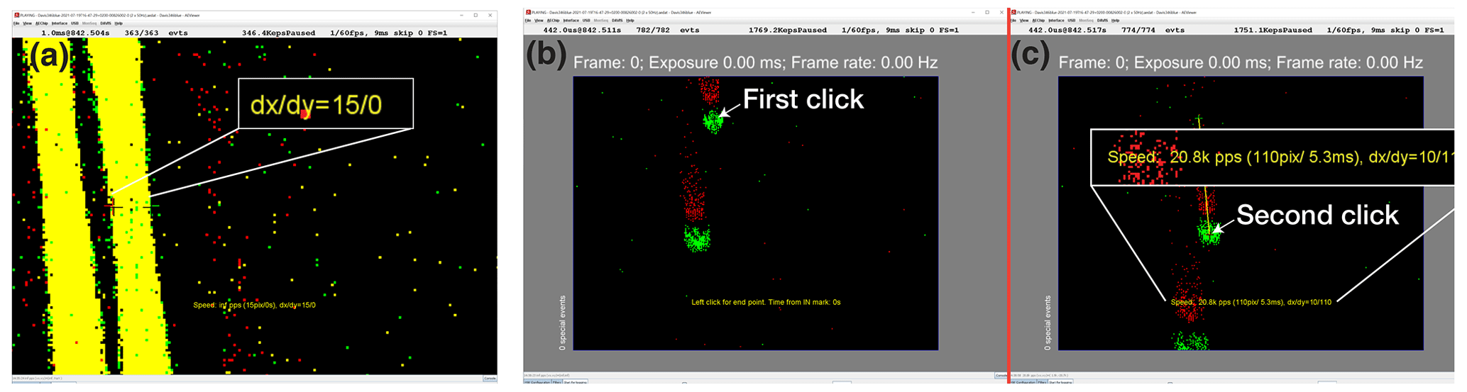
https://amt.copernicus.org/articles/17/335/2024/amt-17-335-2024-f05

Figure 5(a) Diameter measurement. Measurement of the diameter from the DVS recording using jAER. This sample used an HDDG droplet creation frequency f of 100 Hz (2×50 Hz, two-sided). Two droplets passed during the accumulation time. After marking the left and right sides of the hourglass waist with the jAER plug-in Speedometer, it displays the diameter d_r components dx and dy [px]. (b, c) Velocity measurement. Measurement of the velocity from the DVS recording using jAER. (b) We use Speedometer to mark the IN point on the mid-point of the right drop before the drop passes the PoF. (c) Next we mark the OUT point at the midpoint of the drop after the right drop passes the PoF, then Speedometer displays the velocity v_r [kpx s⁻¹].

Figure 5b, c shows the droplet image plane velocity measurement. For this measurement, the event integration time is decreased to about 0.5 ms per frame. Before the drop reaches the PoF (smallest diameter), the playback is paused and the midpoint of the drop is selected by a mouse click (Fig. 5b). After the drop has passed the PoF (Fig. 5c), the playback is again paused and the midpoint of the droplet is again selected. The Speedometer outputs the velocity of the droplet in the image plane as v_r=20.8 kpx s⁻¹.

2.5.3 Computing physical droplet diameter and velocity from DVS image plane measurement

Given the image plane droplet diameter d_r (Sect. 2.5.2), the physical droplet diameter d is calculated from Eq. (1), where M is the calibrated camera magnification (Appendix G):

\begin{matrix} (1) & d [mm] = \frac{d_{r} [px]}{M [px {mm}^{- 1}]} . \end{matrix}

For computing droplet velocity measurement v from v_r, it is useful to use a lens with a long focal length, resulting in a small angle of view (AoV) θ_i, so that the magnification M at the PoF can be assumed to be constant. To further mitigate this effect, it is important to measure the velocity as close as possible to the center of the hourglass. The droplet fall velocity v is calculated from Eq. (2), where Δx_r and Δy_r are the droplet image displacement and Δt is the time interval of the displacement:

\begin{matrix} (2) & \begin{aligned} v [m s^{- 1}] & = \frac{\sqrt{{(Δ x_{r} [px])}^{2} + {(\frac{Δ y_{r} [px]}{\sin α})}^{2}}}{10^{3} \times Δ t [s] \cdot M [px {mm}^{- 1}]} \\ \overset{(*)}{\approx} \frac{Δ y_{r} [px]}{10^{3} \times \sin (α) \cdot Δ t [s] \cdot M [px {mm}^{- 1}]} \\ = \frac{v_{r} [kpx s^{- 1}]}{\sin (α) \cdot M [px {mm}^{- 1}]} . \end{aligned} \end{matrix}

Equation (2) is simplified to the second form when $Δ x_{r} / Δ y_{r} ≪ 1$ and therefore (*) Δy_r≫Δx_r, i.e., when β in Fig. 1b is small. This simplified formula can only be applied if the drop falls vertically for a correct velocity calculation, otherwise, α, which is used for the velocity simulation, would no longer be constant. Figure 1c shows an abstract illustration of a measurement of diameter and velocity from a DVS recording, where the black circles show where the actual droplets are. The circles enclose the bottom edge of the ON events (green points) and OFF events (red points). The tracking points of the droplets that we used for the DVS velocity estimates are the centers of the black circles. Section 2.5.2 shows examples of our actual image plane measurements of diameter and velocity. For the droplet in Fig. 5 using the M and α HDDG values in Table 1, Eq. (1) evaluates to d=15 px $/$ 30.7 px mm $^{- 1} = 0.48$ mm and Eq. (2) evaluates to v=1.8 m s⁻¹.

2.5.4 Ground truth droplet size and velocity determination

Our GT droplet size measurements (not to be confused with ground level) provide the reference data for droplet size and speed that we compare with the DVSD and PARSIVEL measurement results.

The HDDG (Sect. 2.3.2) needle oscillation frequency is adjusted with a function generator and resulted in droplet diameters between 0.3 and 0.6 mm, which in our case corresponded to a droplet creation frequency between 60 and 220 Hz and a flow rate $5.19 \times 10^{- 3}$ g s⁻¹. An ISMATEC REGLO ISM597A Digital peristaltic pump⁷ supplied our HDDG with water at a constant flow rate from a tank placed on top of a KERN 440-35A weighing scale⁸ with 0.1 mg precision. The scale measured the water mass over time to determine the flow rate. By assuming spherical water drops, their diameter is inferred from their mass, which increases with flow rate but decreases with drop creation frequency. The drop creation frequency describes how many drops per second are produced. According to a water droplet model proposed by Beard and Chuang (1987), a spherical assumption is very accurate for submillimeter drops.

The volumetric flow rate $\dot{V}$ is calculated as Eq. (3):

\begin{matrix} (3) & \dot{V} = \frac{Δ m}{ρ Δ t}, \end{matrix}

where ρ=0.997 g cm⁻³ is the density of water, Δm is the change in mass of the water tank (HDDG) or collection cup (IVDG), over a certain period of time Δt. With the flow rate $\dot{V}$ and the assumption of a sphere, the diameter is calculated as Eq. (4):

\begin{matrix} (4) & d = {(\frac{6 \dot{V}}{π f})}^{1 / 3}, \end{matrix}

where f is the drop creation frequency.

We used the IVDG of Sect. 2.3.1 to create larger droplets. To determine the mass of a single droplet, many droplets were counted and collected in a reservoir positioned on the scale whereas the total mass m_tot and the number of drops N were recorded. The volume of a single drop is calculated as

\begin{matrix} (5) & V_{drop} = \frac{m_{tot}}{ρ N} . \end{matrix}

The diameter can then be calculated as

\begin{matrix} (6) & d = {(\frac{6 V_{drop}}{π})}^{1 / 3}, \end{matrix}

where the droplet is assumed to be a sphere. The diameters calculated from Eqs. (4) and (6) are used as GT values to compare with the diameter measurements of DVS.

A separate measurement (Appendix E) shows that the IVDG droplet size distribution varies less than ±1 % over short time scales and less than 3 % over the 20 m measurement duration. For these droplets, the model by Beard and Chuang (1987) predicts a slight average drop deformation owing to drag. However, this average deformation is 0.8 % in the case of 2.50 mm droplets, making them appear to be 2.52 mm when viewed from roughly 30^∘. The average deformation thus introduced only a very small systematic DVS error. A random error was additionally introduced from the vibration of the 2.5 mm droplets.

We computed the GT velocity from the GT diameter using a droplet velocity simulation (Appendix H) for the small HDDG droplets. For the large IVDG droplets, we used the measured velocity from Gunn and Kinzer (1949).

2.5.5 Error analysis

In both experiments, two aspects were considered to determine the propagation of the measurement errors.

The first aspect is the combined measurement uncertainty of the DVSD and GT values, which factors in all uncertainties. For example, an uncertainty in the measurement of the DVSD comes from the limited sensor resolution of the DVSD. Another comes from the uncertainty of α. Together with other uncertainties, we could then calculate the combined standard uncertainty of the DVSD velocity and diameter measurements. The combined GT uncertainty consists of the uncertainty in height, droplet mass, drop creation frequency, etc. According to JCGM (2008), in the case of uncorrelated input quantities x_i, the combined standard uncertainty of a function u(f) can be described as:

\begin{matrix} (7) & \begin{aligned} u (f) \\ = \sqrt{\sum_{i = 1}^{N} {[\frac{d f u (x_{i})}{d x_{i}}]}^{2}} \\ = \sqrt{{[\frac{d f u (x_{1})}{d x_{1}}]}^{2} + {[\frac{d f u (x_{2})}{d x_{2}}]}^{2} + {[\frac{d f u (x_{3})}{d x_{3}}]}^{2} + \dots} \end{aligned}, \end{matrix}

where u(x_i) is the standard uncertainty of the input quantity x_i. The uncertainty is derived either with a Type A evaluation, where the standard uncertainty is evaluated with the experimental standard deviation from repeated observations, or with a Type B evaluation, where the estimated uncertainty is evaluated using our judgment of uncertainty. We used a Type B evaluation, either by using the manufacturer's instrument specifications or by a conservative estimate of the measured uncertainty. A linear approximation of the function is used for each input quantity. A spreadsheet in our online results folder⁹ reports the final uncertainty values computed by our MATLAB scripts.

The second aspect is accuracy, i.e., comparison of the measured values from the DVS with the GT values. This is done by calculating the mean absolute percentage error (MAPE):

\begin{matrix} (8) & MAPE = \frac{100 %}{n} \sum_{i = 1}^{n} |\frac{{GT}_{i} - {ME}_{i}}{{GT}_{i}}|, \end{matrix}

where GT_i is the GT value and ME_i is the measured value.

3 Results

We conducted two series of DVSD experiments, one with the HDDG and one with the IVDG. We used different lenses to make it easier to capture droplets crossing the PoF. The droplets created by the HDDG ranged from 0.3 to 0.6 mm (a diameter of 10 to 20 px on the image), whereas the droplets created by the IVDG were 2.5 mm (17–18 px diameter). In both experiments, the height of the fall was sufficient for the droplets to reach within 97 % of the terminal speed (Appendix H). Because the DVSD sampling area is small, these experiments required patience to collect sufficient data, i.e., such that the recorded droplet showed an hourglass shape in the accumulated playback of the DVS recording. In total we collected N=45 droplets with the HDDG setup and N=27 droplets with the IVDG setup.

To allow comparison, we repeated the experiments with the commercial PARSIVEL laser sheet disdrometer in Table 4. Its larger sampling area (Table 4) allowed us to collect thousands of droplets.

3.1 Results from DVSD

Figure 6 compares the DVSD measurement results performed with the DVS (Sect. 2.5.3) with GT estimates of droplet size and speed (Sect. 2.5.4). The HDDG droplets (green data points) are magnified for better visibility, and the IVDG droplets (purple data points) have a purple histogram beside them, indicating the number of measurement results that overlap. The quantization of the data arises from the quantized droplet size generation and the pixel discretization. Horizontal quantization is caused by the quantized HDDG droplet creation frequencies, which control the diameters of the droplets. Vertical quantization is caused by the low pixel count of the diameter of the droplets in the DVS recording. The speed measurements do not have any significant vertical quantization effects, owing to large pixel displacements (≈ 100 px) and the fine DVS event timestamp resolution of 1 µs. The DVSD results are discussed in Sect. 4.1.

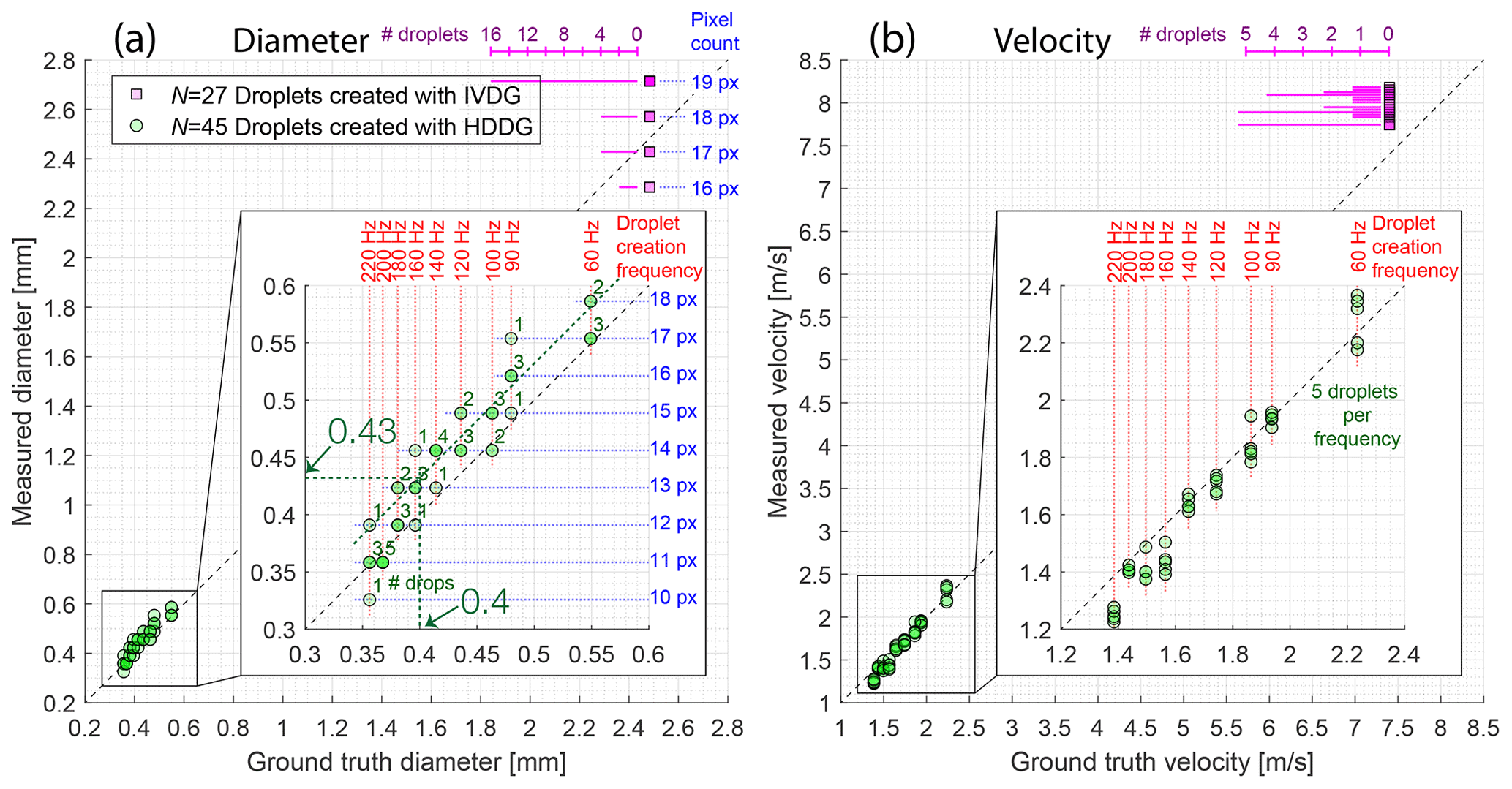
https://amt.copernicus.org/articles/17/335/2024/amt-17-335-2024-f06

Figure 6Main results. DVSD measurement results of droplets compared with GT values, where (a) shows the diameter and (b) shows the velocity. The dashed black line represents a 45^∘ line passing through the origin. Both droplet creation methods are included in the plots. The zoomed plots show droplets created with the HDDG for improved visibility. Numbers adjacent to the points on the left zoomed plot indicate droplet overlaps whereas the zoomed plot on the right has five droplets per frequency. (a) The dashed green lines show a fit to the small droplet data and the measured diameter of 0.43 mm corresponding to the 0.4 mm GT droplets. The IVDG droplets are shown in purple with a histogram for the number of overlapping points. Quantization effects caused by the pixel count or frequency are illustrated as a grid pattern in the plots where the effect is significant. (See Sect. 3 for details.)

Download

We used MAPE to quantify the discrepancy between the ground truth values and the DVS measurements (Sect. 2.5.5). Table 2 lists the diameter and velocity MAPE for both experiments. In all cases, MAPE remains below 7 %, which consists of the DVSD bias to overestimate the droplet diameter.

Table 2MAPE of the DVS measurements compared with GT values, for the diameter and velocity measurements from both experiments.

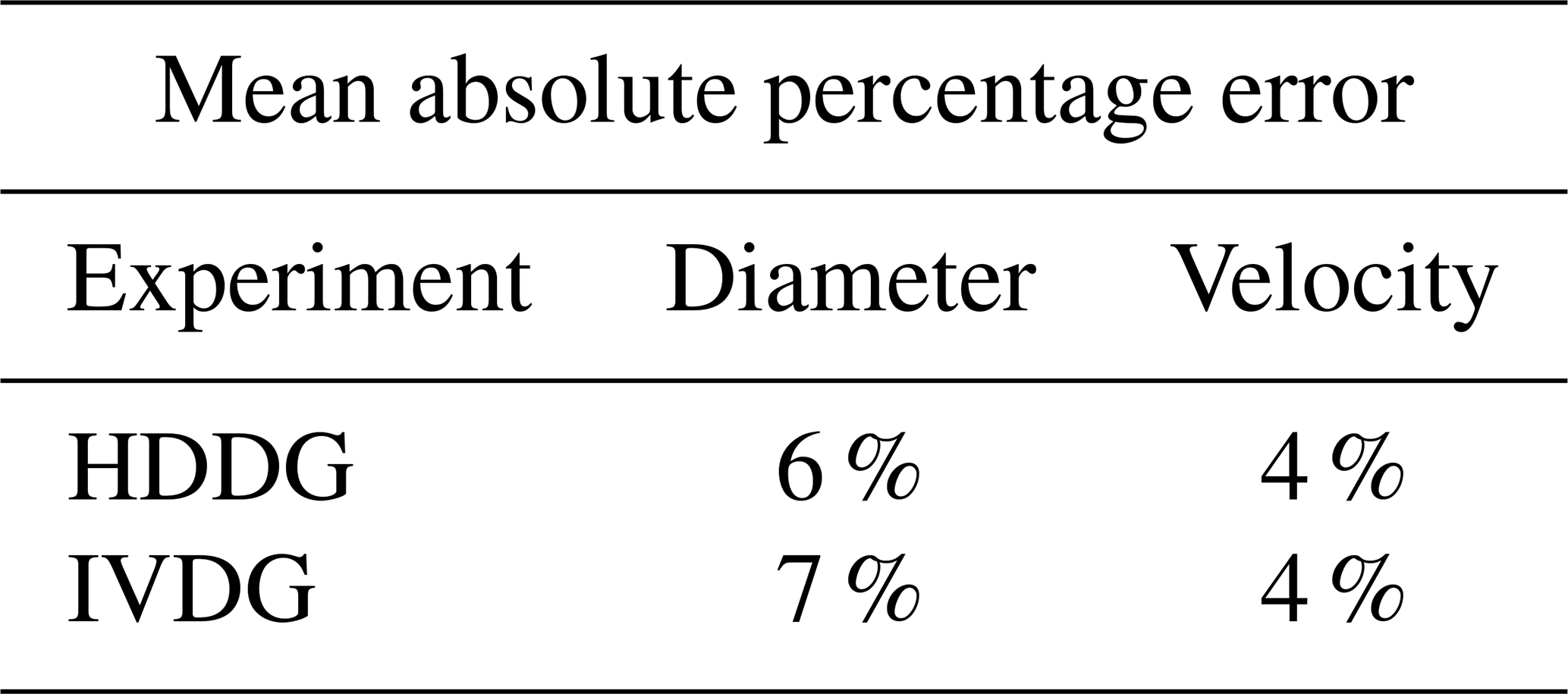
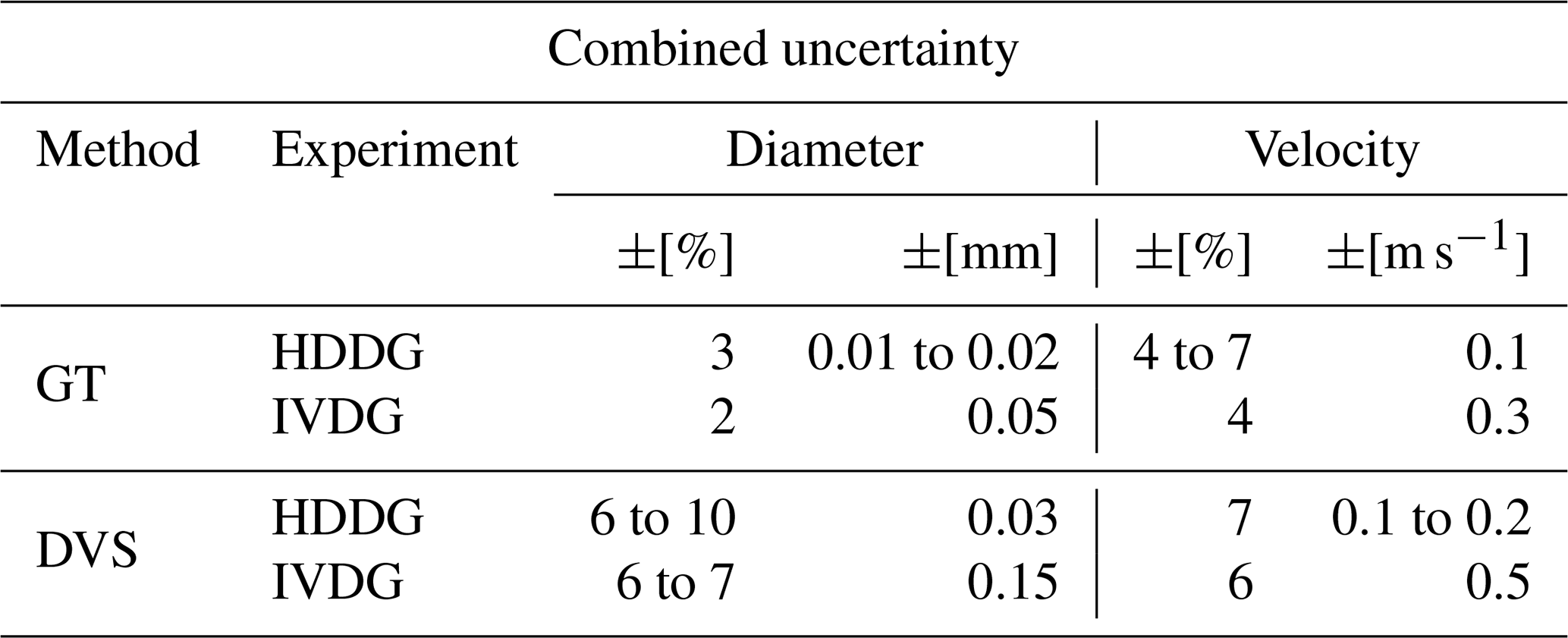
Download Print Version | Download XLSX

Table 3 lists the estimated combined uncertainties of the measured diameter and velocity using the method explained in Sect. 2.5.5. In some cases, a range of uncertainties is given, which means the uncertainty depends on the size of the droplet. The combined uncertainty percentage is largest for the DVS measurement of the smallest droplets created with the HDDG, which had a diameter of 0.35 mm ± 0.03 mm (±10 %). This large uncertainty is caused by the low pixel diameter count (≈ 10 px).

The uncertainty (i.e., precision) of the DVSD diameter and velocity measurements is mainly limited by the spatial resolution of the 346×260 px DVS (Table 3: bottom). The GT diameter uncertainty (see Table 3: top) was mostly caused by the measurement uncertainty of the scale and noise in the droplet generation by the HDDG and IVDG. The GT velocity uncertainty arises from neglecting air turbulence, droplet deformation, and inaccurate sphere model values, i.e., GT droplet diameter estimates from mass flow. The GT droplet diameter and velocity are calculated from their mass and from the simulation respectively (see Sect. 2.3 and Appendix H). Therefore, diameter uncertainty increases velocity uncertainty.

Table 3Percentage and absolute combined uncertainty of the DVS measurements and GT values for diameter and velocity.

Download Print Version | Download XLSX

3.2 Results from the PARSIVEL disdrometer

Figure 7 summarizes the results obtained from the commercial PARSIVEL disdrometer in Table 4 using the HDDG and IVDG setups. Detailed histograms of these results are reported in Appendix C. The PARSIVEL results are discussed in Sect. 4.2.

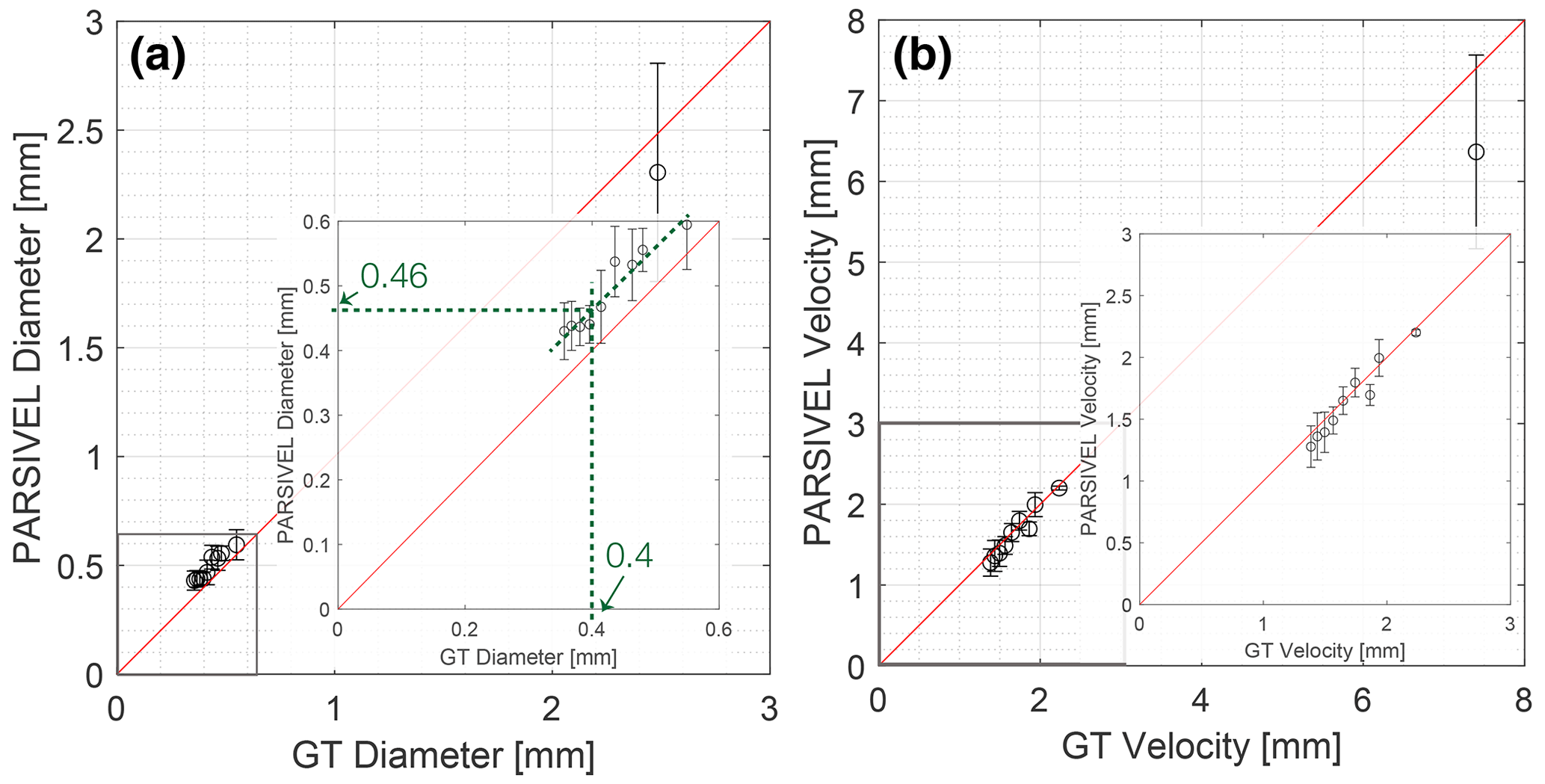
https://amt.copernicus.org/articles/17/335/2024/amt-17-335-2024-f07

Figure 7Summary of results from PARSIVEL in Table 4. Each plot includes a magnified view of the HDDG small droplet results. The red lines pass through the origin with a slope of one to indicate ideal measurements. (a) Diameter measurements versus GT. The green dashed lines show a fit to the small droplet data and the corresponding GT and measured diameter values. (b) Velocity measurements versus GT. See Figs. C1 and C2 for detailed distributions.

Download

Table 4Comparison of disdrometer specifications. Data may not be accurate for the latest models. NA stands for ”not available”.

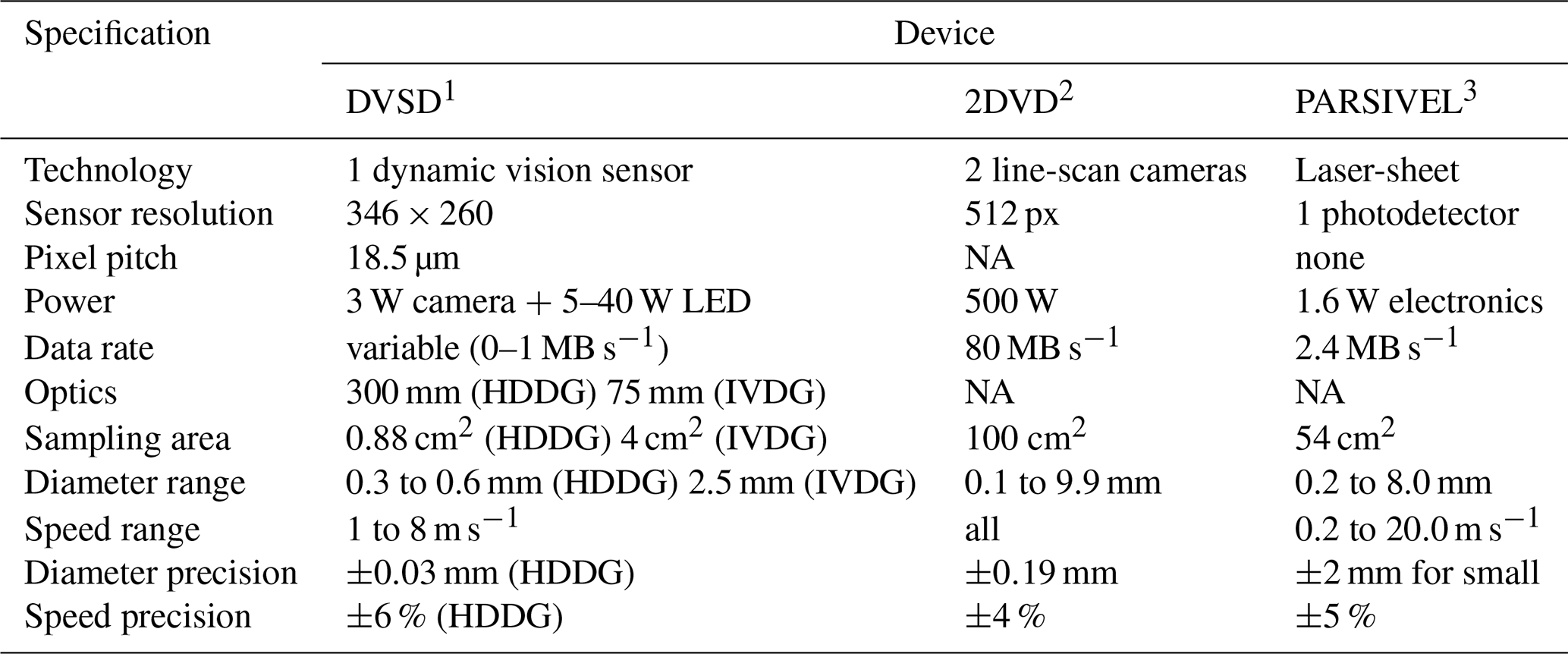
¹ DAVIS346 from https://inivation.com/ (last access: 20 December 2023), based on Taverni et al. (2018) FSI sensor chip. ² Kruger and Krajewski (2002). ³ OTT Hydromet (2016).

Download Print Version | Download XLSX

4 Discussion

4.1 DVSD experimental results

The DVSD results presented in Fig. 6 show excellent linearity over the entire measurement range for both size and speed; the dashed line in each plot has a slope of one and passes through the origin; it lies close to both small and large droplet measurements. Size measurements overestimate droplet diameters by about 8 %, and speed measurements slightly underestimate large droplet speeds.

Although the large droplets were generated and measured differently than the small droplets, the two data sets are very consistent (Fig. 6: green and purple data sets). The offset of the data points from the 45^∘ line (Fig. 6) might be correctable. We believe that it most likely arises from the method of manual marking of the accumulated events to determine the hourglass waist width; this method could slightly overestimate the droplet width. The alternative (an inaccurate M estimate) we consider less likely. Our measurements show from the small droplet fit that GT droplets with diameter 0.4 mm are estimated by the DVSD method to be about 0.43 mm, an overestimate of 8 % in diameter and 24 % in volume. As the HDDG droplets measure about 10 px in the image plane, a single pixel overestimate of droplet width could explain the discrepancy.

We used a shorter lens for the larger IVDG droplets only to allow us to capture the large droplets more easily, as they scattered much more from random wind currents in the staircase than the small droplets from the HDDG. It is possible to obtain better precision of large droplets by using the same lens, but with the trade-off of longer experiment time because fewer pass through the PoFR.

For the IVDG experiment with large droplets, the DVSD method overestimated the 2.5 mm droplets computed GT speed value of 7.4 m s⁻¹ as about 7.8 m s⁻¹, a 5 % overestimate (Appendix H). The droplet velocity distribution appears to have a long tail of droplets with smaller velocities.

4.2 PARSIVEL experimental results

In general, the PARSIVEL measurements in Figs. 7, C1, and C2 agree fairly closely with our GT droplet sizes and velocities and have precision similar to the DVSD, but they consistently show a larger bias to overestimate the small droplet sizes. This size bias is evident in the inset plot of Fig. 7a, where we fitted a line to the PARSIVEL results. The dashed green lines show that GT droplets with diameter 0.4 mm are estimated by the PARSIVEL to be about 0.46 mm, an overestimate of 15 % in diameter and 50 % in volume. By contrast to the DVSD method, which overestimated the 2.5 mm droplet speed by 5 %, the PARSIVEL reported speed of only 6.4 m s⁻¹ (a 16 % underestimate). However a caveat to this result is that the PARSIVEL velocity distribution in Fig. C2 has a long tail of smaller velocities (as from the HDDG measurements) and the modal velocity is about 7 m s⁻¹, which is closer to the GT velocity.

The PARSIVEL IVDG droplet size distribution (Fig. C2) has a long tail for slower droplets, as can also be observed for the DVSD method in Fig. 6, with a significant number of droplets reported to be smaller than the mean. We do not know the cause of these outliers, as the true IVDG droplet size spread is less than 3 % (Appendix E). It is possible that stray updrafts in the staircase slow some of the droplets for both sets of measurements.

4.3 Limitations of experiments

Our experiments were carried out in a controlled environment using two droplet generators, i.e., HDDG and IVDG. However, unlike real rainfall conditions, there were no strong winds. Moreover, the drop jets were localized and did not occlude each other. We do not believe that occlusion would be a problem owing to the optical arrangement, but the droplet tracks could merge or overlap and the droplets in front or behind the PoF could disturb the measurements. Therefore, it is difficult to predict how well a DVSD would perform under windy conditions or with heavy rainfall.

Our hourglass DVSD method (Sect. 2.5.3) requires the droplets to pass through the FoV (see Fig. 1b: left, and Fig. 4: bottom left corner). In an extreme case, the wind could make a droplet trajectory parallel to the line of sight of the camera. In this case, no hourglass would be visible on the DVS recording after an accumulation of events; from the point of view of the DVS, the droplets would appear to shrink and grow while slowly drifting in a random direction.

4.4 Future improvements

Improving the stability of our HDDG should be investigated as our HDDG combined with the tiny sampling area of 0.9 cm² required patience to capture sufficient good droplets to measure (Appendix D). Using near infrared (NIR) illumination should also be tried, as most insects would be blind to it and hence not be attracted to the DVSD, and DVS silicon photodiodes work well with NIR illumination. The ring light could also be made much smaller (and less bright) than the large ring that we used.

In principle, it should be possible to infer the 3D trajectory of the droplet from an algorithm that continuously estimates the diameter and velocity of the droplets. We would base this algorithm on cluster trackers commonly used for other DVS applications (Delbruck and Lang, 2013; Gallego et al., 2020). The tracker would initiate clusters at the top of the FoV, and then use brightness change events to track the droplets, while measuring their velocity and diameter. A simple set of plausibility checks on the cluster path and cluster size at the start, middle, and end of the path and a fit to the hourglass diameter samples could provide the image plane droplet measurements along with their uncertainties.

The size of the sampling area plays an important role in how quickly a DSD can be obtained. The sampling area of the DVSD decreases slightly with increasing drop size, because the droplets must be fully inside and pass through the FoV. Therefore, a correction will be needed to estimate the DSD to account for the smaller fraction of larger droplets that are measured. This correction would be less important for a larger sampling area.

If our DVS were required to have the same sampling area as the OTT Parsivel² (see Table 4), a reduction in focal length would be necessary, but would increase the current 0.35 mm drop size uncertainty from 10 % (Table 3) to 75 %. However, these limitations are a result of the low spatial resolution of our prototype camera. Megapixel DVS are already available (Suh et al., 2020; Finateu et al., 2020). With a megapixel DVS, the 0.35 mm droplet size uncertainty would be about 20 % while matching the 54 cm² sampling area of the OTT Parsivel² (Table 4). Table G1 shows that a 1280 × 720 px DVS with 5 µm pixels (Finateu et al., 2020) using a focal length of 50 mm and a working distance of 75 mm would provide a sampling area of 48 cm² and 0.3 mm droplets would still occupy 4 px. Given the subpixel resolution provided by fitting to the hourglass contour of the accumulated events, the droplet size precision would probably be better than 10 %.

4.5 Comparing DVSD with other optical disdrometers

Table 4 compares the specifications of our current DVS prototype with those of the OTT Parsivel² and 2DVD. Existing optical disdrometers measure the size of the droplets by the size of the 1D occlusion (2DVD) or the decrease in the intensity of light (PARSIVEL). The DVSD takes advantage of the ability of DVS to finely measure the velocity of the droplet across the plane of focus and uses the PoF to locate the droplet in space for unambiguous size measurement.

The measurement uncertainty of the DVSD is within a range similar to that of other optical disdrometers; field experiments with co-located instruments resulted in a diameter error of about 5 %–11 % in small drops (D₀= 1–2 mm) and the error varies from approximately 8 % to 4.5 % at D₀=1.5 mm from a 1 min to a 10 min sampling time (Jaffrain and Berne, 2012; Chang et al., 2020).

Johannsen et al. (2020) reported difficulty with long-term measurements using PARSIVEL and 2DVD because of drift and insect and spider debris accumulating in optical housings. The simpler free-space optical arrangement of the DVSD could be advantageous in avoiding these problems. Speed is measured by the time of passage between nearby light sheets (2DVD) or by the time that a single light sheet is occluded (PARSIVEL) (Johannsen et al., 2020). Both techniques require high sample rates because droplets that fall at a terminal speed pass through any given point in a few hundred microseconds. For example, a 1 mm droplet falling at its terminal speed of 4 m s⁻¹ (Appendix H) passes by in only 250 µs. The 1 µs time resolution of DVS allows very accurate measurements of droplet speed in the image plane, but at a low camera data rate of 5000 to 50 000 brightness change events per droplet, which could easily be processed by an embedded microcontroller.

5 Conclusions

Our paper proposes an innovative way of measuring droplets using an activity-driven DVS event camera that observes the droplets falling through a shallow DoF. Our results demonstrate the feasibility of this DVSD method for droplets ranging from 0.3 to 2.5 mm, covering most of the real rainfall range. Droplet size and velocity measurements from the DVSD have a maximum of 7 % MAPE compared with the ground truth from the drop generator. The droplet size uncertainties of the DVSD measurements and GT values are 10 % and 3 % respectively, whereas the droplet velocity uncertainties are both 7 %. The uncertainty of our prototype is encouraging because we expect substantial potential for improvement from higher resolution event cameras and automated high-throughput processing methods. Our results have smaller bias to overestimate small droplet sizes than the commercial PARSIVEL disdrometer, which is important for estimating water volume from light rain events.

With our strongest magnifying lens, our DVSD prototype, under laboratory conditions, surpasses SoA disdrometers in terms of precision, although the sampling area is much smaller, as Table 4 shows. For future work, our aim is to increase the sensor resolution and capture real rainfall data with comparisons with SoA disdrometers.

Today, DVSDs would be expensive because of the low-volume production costs of DVS cameras. However, mass production for DVS applications in consumer electronics will rapidly decrease production cost and improve the resolution and quality of DVS cameras. The absolute droplet size and velocity depend only on image-plane measurements of the event stream and the values of two stable and easily measured parameters, the magnification M and the camera angle α. The use of only a single camera should reduce cost and requirements for precise alignment. A DVSD based on a low-power, inexpensive embedded Linux microcomputer could be developed that can autonomously estimate droplet diameters and velocities in real time while surviving harsh weather conditions in remote areas disconnected from the power grid. The rain-driven computation and simple optical and lighting requirements of a DVSD would be a great advantage compared with alternative optical disdrometers that sample at a constantly high rate and require more complex optical and lighting arrangements.

Appendix A

The appendices consist of the following:

Appendix B shows photos of our experimental setups described in Sect. 3.1.
Appendix C provides details of the PARSIVEL results presented in Sect. 3.2.
Appendix D provides additional useful methodology for testing the stability of the HDDG described in Sect. 2.3.2.
Appendix E discusses the uniformity and long-term stability of the IVDG from Sect. 2.3.1.
Appendix F explains how we optimized our droplet illumination.
Appendix G explains our calibration of the optical magnification of the camera M, and provides tables of computed optical parameters for the experiments and for future DVSDs.
Appendix H explains our model of droplet speed versus fall height and droplet diameter, which we used to obtain our GT speed from mass and to ensure that the droplets fell close to the terminal speed.

Appendix B: Photos of experimental setups

Figures B1 and B2 show photos of our HDDG and IVDG experimental setups described in Sect. 2.4.

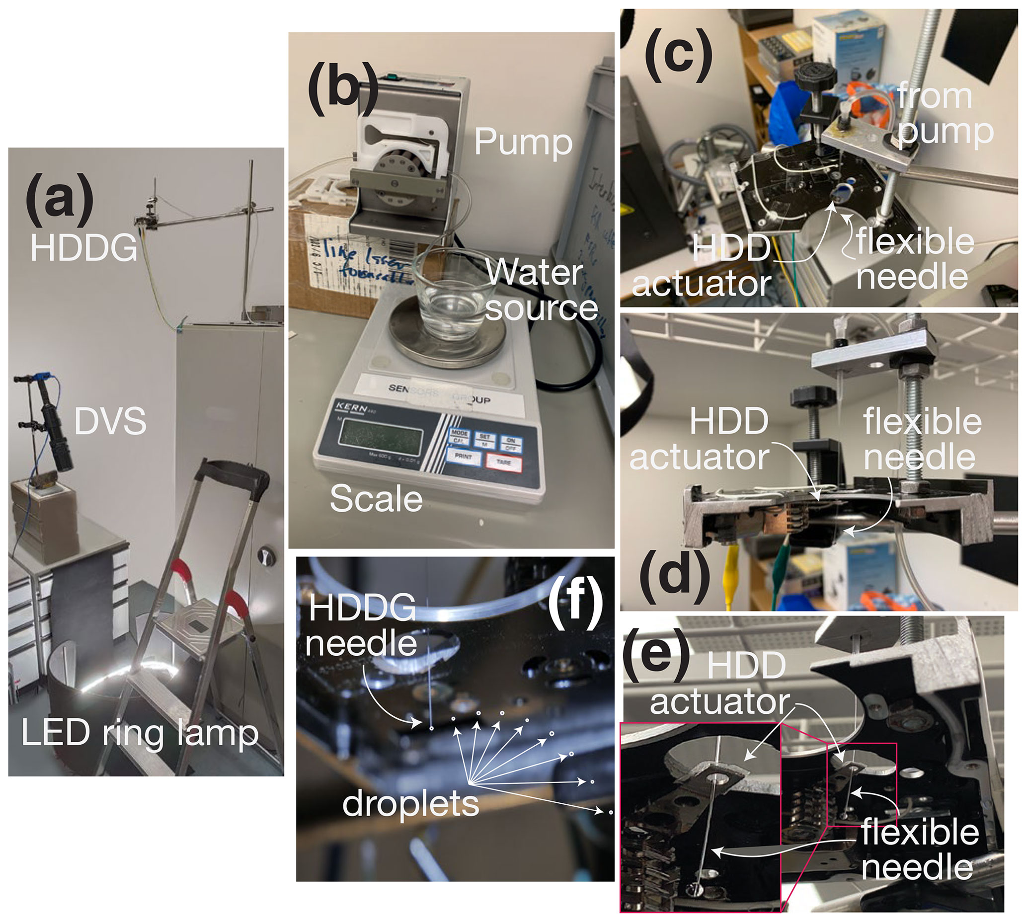
https://amt.copernicus.org/articles/17/335/2024/amt-17-335-2024-f08

Figure B1Pictures of the HDDG experimental setup. (a) Overview of the whole HDDG setup. (b) Peristaltic pump, scale, and water tank. (c, d, e) HDDG drop generator from three different perspectives. (f) Stream of droplets created by the HDDG, taken with a single short exposure.

Download

https://amt.copernicus.org/articles/17/335/2024/amt-17-335-2024-f09

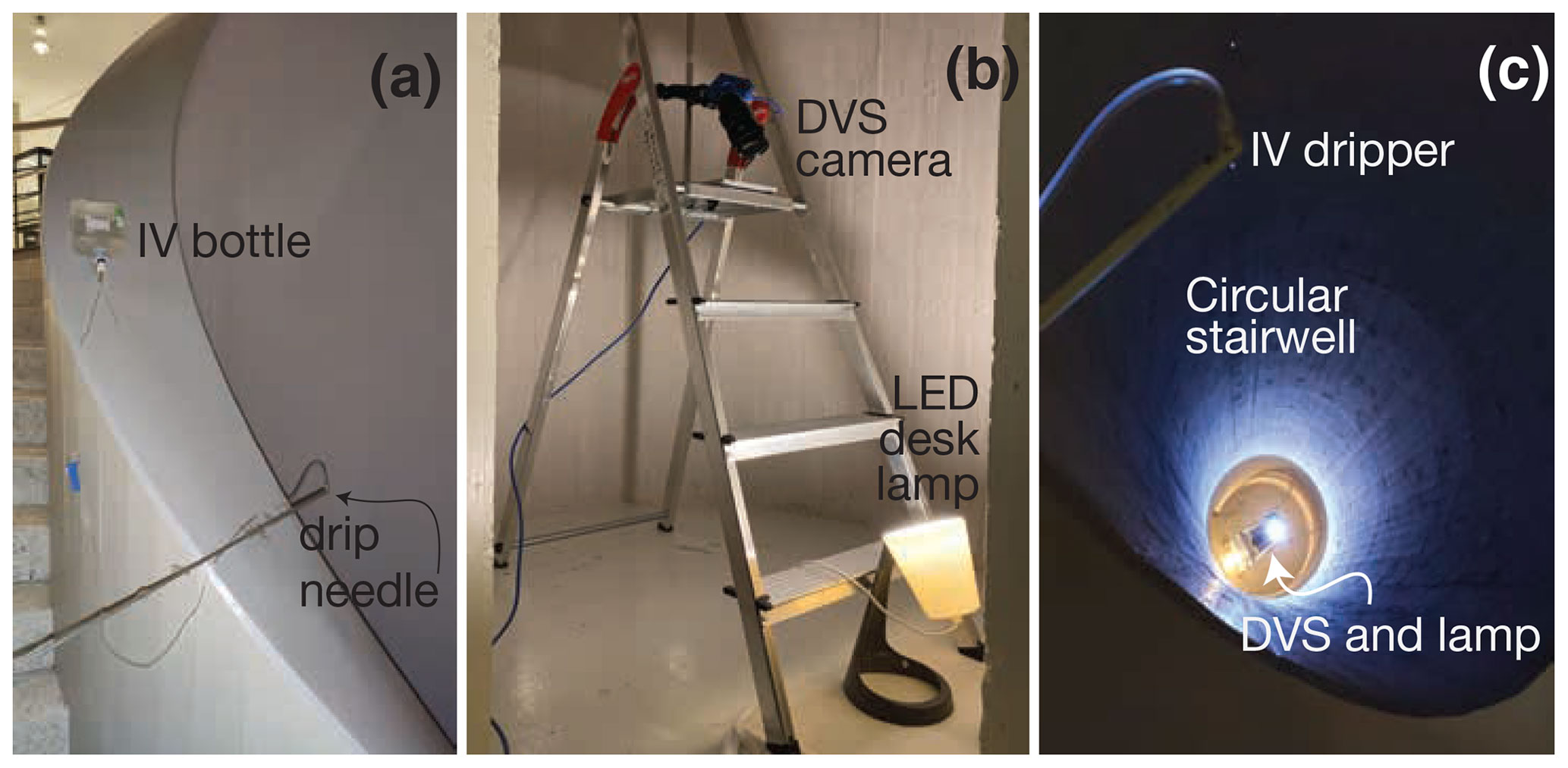
Figure B2Pictures of the IVDG experimental setup. (a) IVDG drop generator with water source and rod holding the needle. (b) DVS camera and lighting setup. (c) Tube inside the staircase with a fall height of 10 m with the IV dripper at the top and the DVS camera and the lighting setup at the bottom.

Download

Appendix C: Details of PARSIVEL results

The sampling area of the PARSIVEL is more than 60× larger than with the DVSD (Table 4) so we could measure hundreds (IVDG) or thousands (HDDG) of droplets under each source droplet condition.

The PARSIVEL HDDG measurements took about 2 m for each droplet size and measured an average of about 3000 droplets. The IVDG measurement took 1200 s to record 149 droplets, an average of one every 8 s, which is about 10× less than the source rate of about 1 Hz. The spatial spread of droplets over the fall of 10 m was still enough to cause many of them miss the 54 cm² PARSIVEL sampling area.

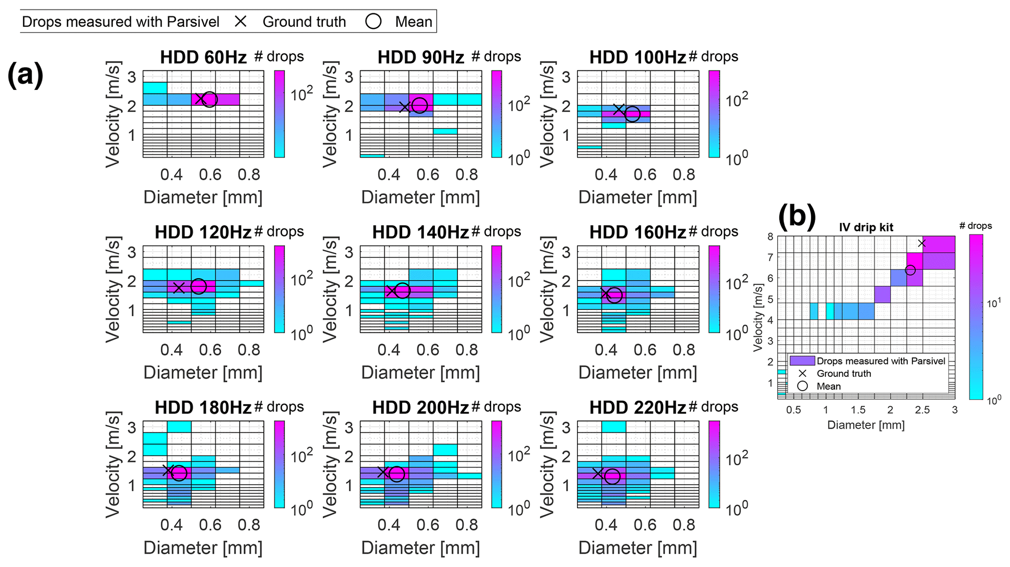
https://amt.copernicus.org/articles/17/335/2024/amt-17-335-2024-f10

Figure C1Results from PARSIVEL in Table 4 plotted as 2D distributions. The GT droplet size and speed are indicated by an X in each plot. The means of the distributions are indicated by an ◦. The bins are the standard classes produced by the device. (a) Results from the HDDG. (b) Results from the IVDG.

Download

Figure 7 summarizes the PARSIVEL measurements. Each Fig. C1 plot shows a distribution of measured droplet size and speed for a single GT droplet size, which is marked by an X in the plot. The mean of each droplet size and speed measurement is marked by an ◦. The GT droplet sizes were measured using the procedure in Sect. 2.5.4. Figure C2 plots the same data as 1D histograms on a linear scale to better see the distribution shapes.

Data collected from the PARSIVEL disdrometer shown in Fig. 7 (see also Figs. C1 and C2) are binned by the device into droplet size and velocity classes. From the counts of droplets in these classes and the bin size and speed values we computed the mean values shown in Fig. 7.

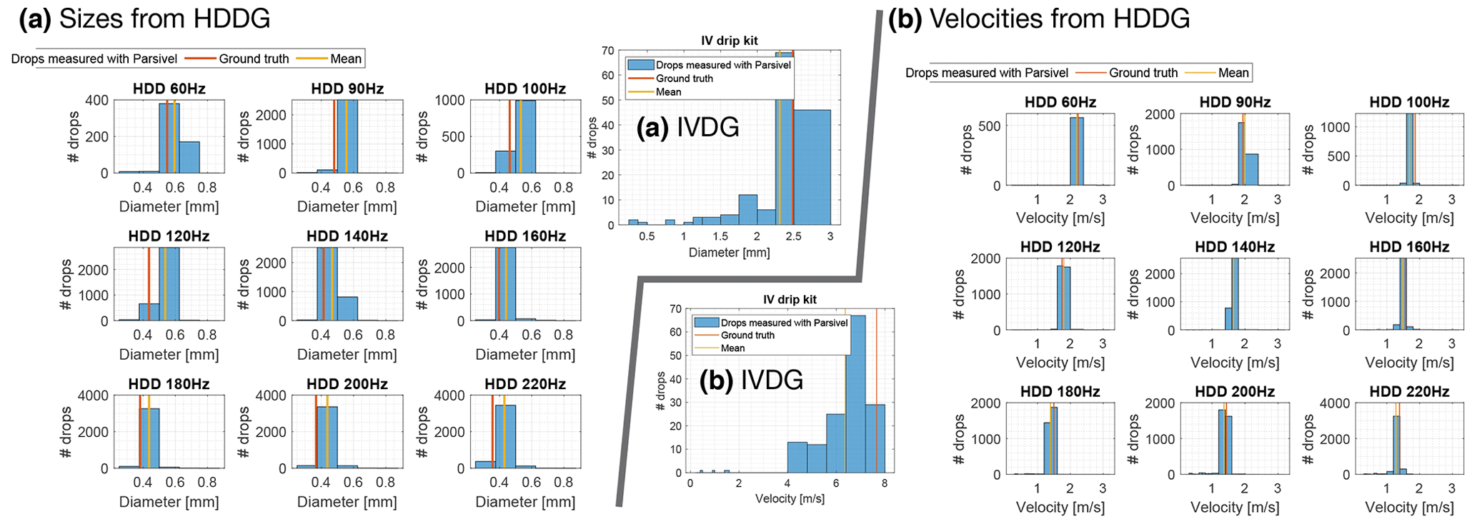
https://amt.copernicus.org/articles/17/335/2024/amt-17-335-2024-f11

Figure C2Results from PARSIVEL in Table 4 plotted as 1D histograms. The measured ground truth droplet size and speed are indicated by a vertical red line in each histogram. The mean values are indicated by the vertical yellow line. The bins are the standard classes produced by the device. (a) Droplet diameters. (b) Droplet velocities.

Download

Appendix D: Testing the stability of the hard disk drop generator with a strobe light

We observed that the HDDG droplet jet continually changed direction a little. The jet moved in apparent cycles. So we had to be patient and lucky that the jet landed in the DVS measurement area. This is what we mean by “unstable drop generation by HDDG” in Sect. 4. There are probably several effects that caused this behavior, i.e., irregular water flow from the pump, a loosely attached needle (so that it can rotate and tilt slightly), and air currents. We believe that air currents only played a minor role and that the most likely culprit is the circular hole in the HDD arm that couples it with the needle (Fig. B1e).

Under our lighting and with HDDG drop generation frequencies above 20 Hz, any errors with the HDDG drop release are too fast to be seen with the naked eye. To test the HDDG drop release, we used a custom-built strobe light to illuminate the oscillating needle. For the initial experiments, the goal was to create one drop per cycle, which meant that the drop stream was one-sided. For higher frequencies, it was impossible to tell if a drop is released every one or every two cycles. We built an Arduino-driven LED strobe light to check the drop creation frequency using the principle of aliasing. We set the strobe light frequency to the same as the desired drop creation frequency for 2 s, and for another 2 s, the strobe frequency was half of the desired drop creation frequency. If the distance between successive droplets (see Fig. B1f) changes between the droplets when illuminated with the two different strobe frequencies (i.e., the distance doubles when the strobe light is flashing at half the desired drop creation frequency), only one drop is released every second cycle. If the distance between the droplets stays the same, one droplet is released per cycle, which is desired.

Appendix E: Testing the uniformity of the IVDG droplets

To measure the uniformity of the droplets produced by the IVDG (Sect. 2.3.1), we recorded the droplets falling from the needle tip with a DVS camera aimed near the tip of the needle. We recorded the event rate over time and used the distinct peaks in event rate produced by each droplet to measure the droplet interval with a resolution of 3 ms.

Figure E1 shows the resulting droplet interval distribution. This measurement took place over 16 min and recorded a total of 1200 droplets. During any short time, the droplet dimension variation is less than ±1 %. Figure E1b shows that the droplet interval gradually increased over time. The IVDG measurements in Sect. 3 were taken over 20 min; thus, they probably had the same slow decrease in droplet size. The total interval increase of 10 % over 16 m would correspond to a droplet diameter decrease of about 4 % over the 20 m measurement period of our IVDG experiments.

https://amt.copernicus.org/articles/17/335/2024/amt-17-335-2024-f12

Figure E1IVDG interval versus time (a) and droplet interval distribution (b).

Download

Appendix F: Optimizing the droplet lighting

https://amt.copernicus.org/articles/17/335/2024/amt-17-335-2024-f13

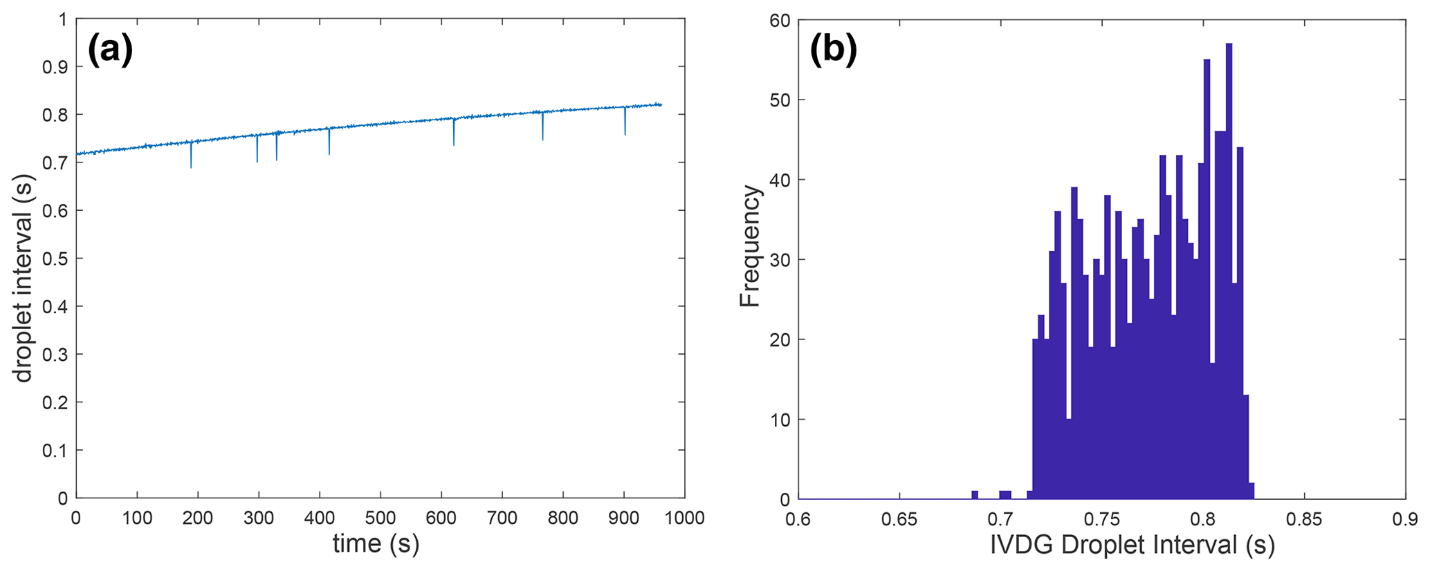
Figure F1Drop illumination from an LED ring with six lamps, with (a) showing a drop with pronounced edges and (b) showing a drop with less pronounced edges.

Download

Water droplets refract light in the same way that convex glass elements do, namely, toward the middle. This property of drops was used to determine a good lighting setup for DVS. To test this optical phenomenon, we took a dispensing needle and attached a tiny water drop to its end and took a photograph of it. We altered the distance between the circular light source and the PoF until we were satisfied with the brightness of the drop edge. We note here that the ring light that we used was much too large for our sampling area; we could have used one that was smaller by a factor of about 100 in area. Figure F1 shows the drop illumination for two different distances of the light source from the droplet. In Fig. F1a the edges of the drop are clearly pronounced, whereas in Fig. F1b the edges are weak. It is important to align the light source correctly as in Fig. F1a, so that the edges of the droplet are well pronounced at the PoF. The light source used for Fig. F1 was a ring light configuration with six LED bulbs. The light source used for the HDDG experiments was a ring light with a LED strip. However, the phenomenon is still thesame. For the IVDG setup we were forced to use a singleLED desk lamp owing to limited stairwell space. This single lamp was not ideal because it caused a bright refraction inside the droplet, but we could still distinguish the outline of the events produced by the droplet edge to measure the droplet diameter.

Appendix G: Optical and geometrical calibration

The camera extrinsic and intrinsic geometry and optics must be calibrated to compute the physical diameter and velocity measurement from DVS image plane measurements.

G1 Camera angle α

The parameter α is used in Eq. (2). It is the angle between the line of sight (LoS) of the camera and the vertical yz-plane (see Figs. 1B: left and G1). We measured α with a smartphone accelerometer.

G2 Magnification M

The magnification M in pixels per millimeter describes how large a certain distance in reality on the PoF would appear on the DVS recording and vice versa. The magnification calibration is done by recording a miniature checkerboard calibration chart held at the PoF with the DVS. M_meas is measured by dividing the number of pixels occupied by a checkerboard square by the checkerboard square size in mm. A comparison of measured M_meas and calculated M_calc values is listed in Table G1 and they are in good agreement. The discrepancy could arise from inaccurate manufacturer focal length specification. We used the measured M_meas value.

G3 Field of view, sampling area, and resolution

Figure G1 shows the geometry of the FoV and the AoV, which are important for measuring the velocity on the DVS camera, and the sampling area. Table G1 summarizes the data of this section. The source spreadsheet is available as an online spreadsheet¹⁰.

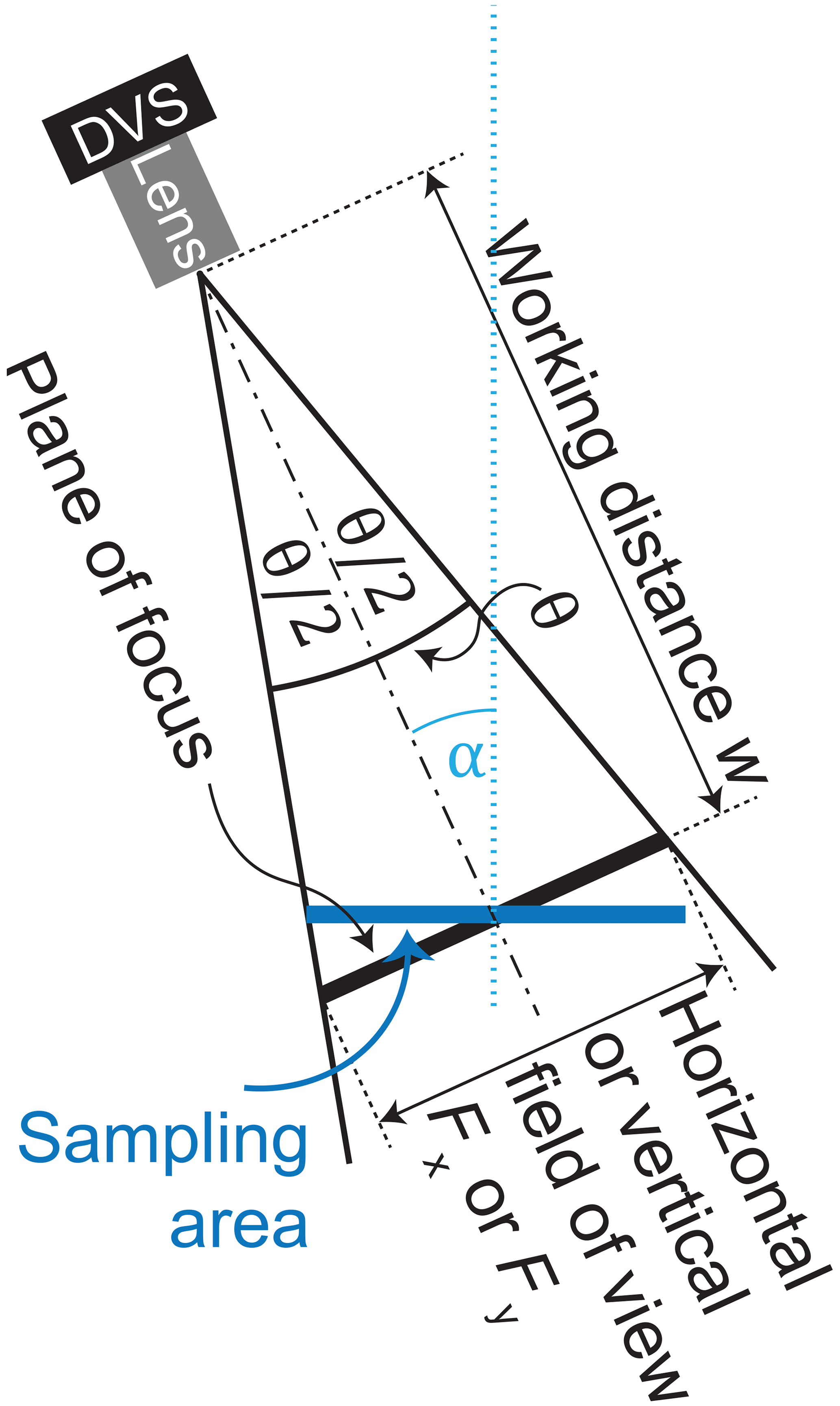
https://amt.copernicus.org/articles/17/335/2024/amt-17-335-2024-f14

Figure G1Illustration of the FoV F_x and F_y and sampling area of the camera including the corresponding AoV θ_x and θ_y. The camera angle α is also illustrated.

Download

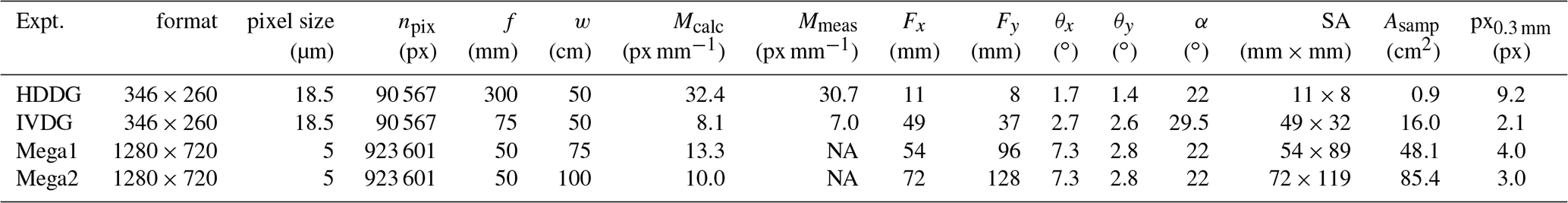
Table G1HDDG and IVDG geometrical and optical parameters, including possible future megapixel DVS cameras with 5 µm pixels. NA stands for ”Not available”.

Download Print Version | Download XLSX

The AoV θ can be calculated with the working distance w, horizontal FoV F_x and vertical FoV F_y, which are both defined at the PoF. This calculation is done by Eq. (G1):

\begin{matrix} (G1) & θ_{i} = 2 \arctan (\frac{F_{i}}{2 w}), \end{matrix}

where F_i is calculated with the measured magnification M in pixels per millimeter (Appendix G) and one less than the number of pixels in the according pixel direction of the DVS:

\begin{matrix} (G2) & \begin{array}{l} F_{x} [mm] = \frac{345 [px]}{M} \\ F_{y} [mm] = \frac{259 [px]}{M} \end{array} \end{matrix}

Because the angles θ_x and θ_y are small, an assumption of a parallel FoV is appropriate (θ_i=0). The magnification M in the vicinity of the PoF can be assumed to be constant, which simplifies the velocity calculation.

G3.1 Sampling area

The droplet collection sampling area A_samp in Table 1 is computed from Eq. (G3), which accounts from the camera angle α:

\begin{matrix} (G3) & A_{samp} = F_{x} F_{y} \cos α = {SA}_{x} {SA}_{y} . \end{matrix}

G3.2 Resolution

Table G1 lists px_0.3 mm, which is the number of pixels occupied by a tiny 0.3 mm droplet. Table G1 also lists optical parameters for future DVSDs that use a megapixel DVS with smaller pixels, e.g., Finateu et al. (2020).

G4 Depth of field

The DoF is approximately given by Eq. (G4):

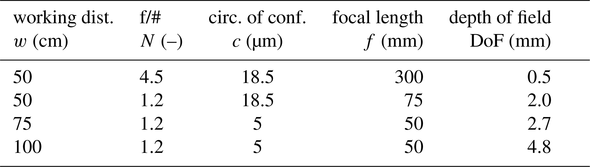
\begin{matrix} (G4) & DoF = \frac{2 w^{2} N c}{f^{2}}, \end{matrix}

for a given circle of confusion c, focal length f, f number N, and working distance w (Allen and Triantaphillidou, 2012). N is the ratio of f to the diameter of the entrance pupil. c is the diameter of the largest image plane spot that is indistinguishable from a point. For this work, we take c to be the DVS pixel size 18.5 µm as a means of scaling the arbitrary circle of confusion size to the DVS resolution.

Table G2 summarizes the data of this section. The source spreadsheet is available at Footnote 10. A smaller DoF results in a more pronounced hourglass shape for the accumulated DVS events produced by a droplet. Equation (G4) shows that we can minimize the DoF by using a fast lens (small N) and by maximizing the ratio of focal length to working distance ( $f / w$ ).

Table G2Depth of field computations, including possible future DVS cameras with 5 µm pixels.

Download Print Version | Download XLSX

Appendix H: Numerical speed simulation of falling drops

A numerical velocity simulation was used to analyze the dynamic behavior of a falling droplet with diameters up to 2.5 mm. We used the results of the simulation to determine the terminal speed and the fall height needed to reach any desired final speed, ideally close to the terminal speed. Being close to the terminal speed ensures that DVS captures drops with properties similar to real rainfall, and ensures that an uncertainty in height measurement leads to a small deviation from the predicted velocity by simulation. We determined the GT droplet speeds from the simulation, except for the large IVDG droplets where we used the Gunn and Kinzer (1949) measured speed value.

For simulation, all water drops were assumed to be solid and smooth spheres, which is an eligible approximation especially for drops less than 1 mm that do not experience any significant deformation according to Beard and Chuang (1987) and Van Boxel (1997). Any effect of deformation or vibration due to air drag and turbulence was neglected. Literature values for the air and water properties were used, where the air and water temperatures for 20 and 25 ^∘C were interpolated to 22.5 ^∘C.

The differential equation for the velocity simulation consists of a drag force, gravity, and acceleration term. The differential equation is numerically solved using the Euler forward method. The relation between drag coefficient and Reynolds number for solid spheres is used, which was fitted to the model of Yang et al. (2015) with the empirically obtained data of Brown and Lawler (2003).

Numerical velocity simulation is used as the velocity GT to compare velocity measurements with DVS. To determine the accuracy of the simulation, the terminal velocity of the simulation is compared with the accepted reference data of Gunn and Kinzer (1949). The results show that they are very close to each other for drops up to 1 mm. However, for larger drops, the simulation predicts slightly higher velocities; for the 2.5 mm drops created with the IVDG, the simulation predicts 7.9 m s⁻¹ whereas Gunn and Kinzer (1949) measured 7.4 m s⁻¹.

Figure H1a plots the model for different drop diameters. For larger droplets, the fall height must be higher to reach the terminal velocity. Moreover, the terminal velocity for larger drops is larger than for smaller ones. Figure H1b compares the simulated velocity and the measured data from Gunn and Kinzer (1949). The simulation starts to differ from the data for droplets with a diameter above 1.5 mm.

According to our simulation, a fall height of 2 m is sufficient for drops with a diameter of up to 0.6 mm to reach 99 % of the terminal velocity, whereas for 2.5 mm drops, a fall height of 10 m is necessary to reach 97 % of the terminal velocity (see Fig. H1a). Thus, a fall height of 2 m was used for the HDDG experiment and 10 m was used for the IVDG experiment.

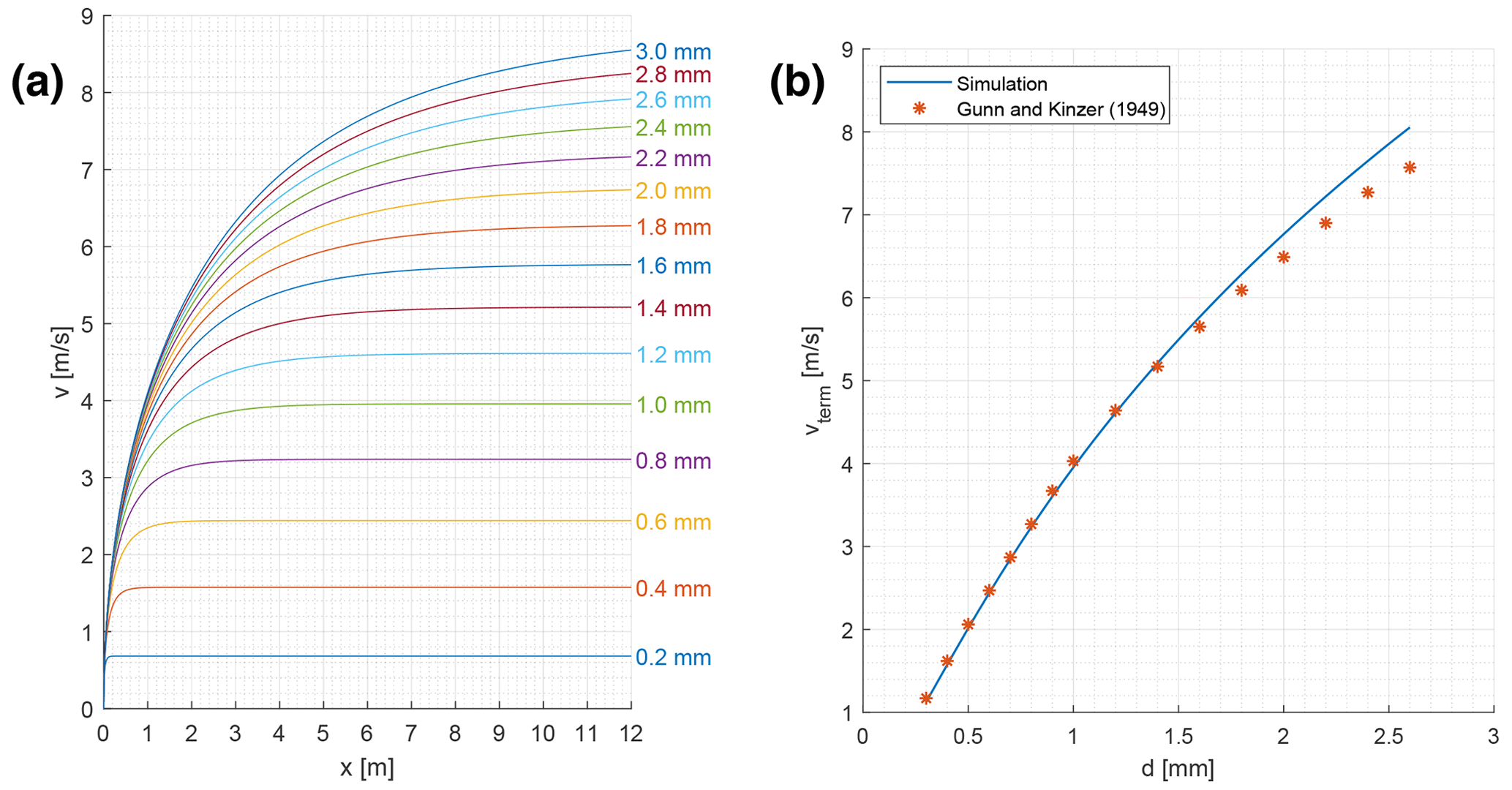
https://amt.copernicus.org/articles/17/335/2024/amt-17-335-2024-f15

Figure H1Falling droplet simulation results. (a) Velocity simulation for a fall height up to 12 m and for different drop diameters (written on the right side); vertical displacement y versus velocity v. Literature values for the density of air ρ_air, kinematic viscosity of air ν_air, and the density of water ρ_water were used for a temperature of 20 ^∘C. (b) Comparison of the terminal simulated terminal velocity with the data of Gunn and Kinzer (1949); diameter d versus terminal velocity v_term. Literature values for the density of air ρ_air, the kinematic viscosity of air ν_air, and the density of water ρ_water were used for a temperature of 20 ^∘C.

Download

H1 Details of droplet speed simulation

The following describes the details of the model used to simulate the speed of a falling water droplet. The goal is to find the velocity v of the drop as a function of the vertical distance y the drop has traveled from its initial position for any given diameter d. This model allows us to determine the terminal speed and the required fall height to reach a certain fraction of the terminal speed v_term, ideally close to the terminal speed. Our model is based on Yang et al. (2015).

The drag force F_D acts on a falling water drop that eventually reaches equilibrium at terminal velocity v_term with the gravitational force mg. The drag force is defined as Eq. (H1):

\begin{matrix} (H1) & F_{D} = \frac{1}{2} ρ_{air} c_{D} (Re) A v^{2} = k (Re) v^{2}, \end{matrix}

where c_D is the drag coefficient depending on the Reynolds number Re, ρ_air is the density of air, A is the area facing the fluid (for spheres: $A = π {(\frac{d}{2})}^{2}$ ) and $k = \frac{1}{2} ρ_{air} c_{D} A$ . The equation of motion can be derived as Eq. (H2):

\begin{matrix} (H2) & m a = m g - F_{D} = m g - k (Re) v^{2}, \end{matrix}

where a is the acceleration, v is the velocity, and g is the gravitational acceleration. Equation (H2) can be rewritten as a differential equation Eq. (H3):

\begin{matrix} (H3) & m \ddot{y} = m g - k (Re) {\dot{y}}^{2}, \end{matrix}

where y describes the vertical displacement of the droplet from the droplet generator. As mentioned above, the drag coefficient c_D depends on the Reynolds number Re. The curve fit for the drag coefficient derived by Yang et al. (2015) is used for the simulation, which is expressed as Eq. (H4):

\begin{matrix} (H4) & \begin{array}{l} x = \frac{\ln (1 + Re)}{10} \\ α = [1 - \exp (- 3.24 x^{2} + 8 x^{4} - 6.5 x^{5})] \cdot \frac{π}{2} \\ c_{D} = \frac{24}{Re} \cdot {(1 + \frac{3}{16} Re)}^{0.635} \cdot \cos^{3} α + 0.468 \cdot \sin^{2} α, \end{array} \end{matrix}

where the Reynolds number Re is defined as

\begin{matrix} (H5) & Re = \frac{ρ v L}{μ} = \frac{v L}{ν}, \end{matrix}

where ρ is the density of the fluid, v is the flow velocity, L is the characteristic length (in this case L=d), μ is the dynamic viscosity of the fluid, and ν is the kinematic viscosity of the fluid. Equation (H4) is a very good approximation for Reynolds numbers Re<2e5, which water drops never exceed, according to Gunn and Kinzer (1949).

MATLAB code to compute discrete time updates of these equations is available from our website (see section “Code and data availability”).

Code and data availability

For MATLAB analysis code and raw source data see https://sites.google.com/view/dvs-disdrometer/home (Micev et al., 2023).

Video supplement

The videos show the operation of the HDDG and slow motion jAER replays of events caused by droplets passing through the plane of focus rectangle. See https://sites.google.com/view/dvs-disdrometer/home (Micev et al., 2023) for videos.

Author contributions

JS and KM performed most of the experimental work and data analysis. AA performed initial experiments to establish the concept. TD and JR conceived and supervised the project. All authors contributed to the first draft. TD prepared the final manuscript.

Competing interests

The contact author has declared that none of the authors has any competing interests.

Disclaimer

Publisher’s note: Copernicus Publications remains neutral with regard to jurisdictional claims made in the text, published maps, institutional affiliations, or any other geographical representation in this paper. While Copernicus Publications makes every effort to include appropriate place names, the final responsibility lies with the authors.

Acknowledgements

This project was supported by EAWAG and the Institute of Neuroinformatics – ETH/UZH.

We thank Juan Pablo Carbajal (Ostschweizer Fachhochschule, https://www.ost.ch/de/, last access: 20 December 2023) for catalyzing this collaboration, Konrad Schindler (ETH Zurich, https://prs.igp.ethz.ch/group/people/person-detail.schindler.html, last access: 9 January 2024) for supervising the undergraduate student projects, Gemma Taverni (formerly UZH-ETH, https://www.ini.uzh.ch/en.html, last access: 20 December 2023) for help with initial feasibility studies, Sebastian Kosch (https://aldusleaf.org/, last access: 20 December 2023), Nasser Ashgriz (University of Toronto, https://www.mie.utoronto.ca/faculty_staff/ashgriz/, last access: 20 December 2023), and Reinhard Loidl (UZH-ETH, https://www.ini.uzh.ch/en.html, last access: 20 December 2023) for their advice on building the HDDG.

Review statement

This paper was edited by Alexis Berne and reviewed by Dhiraj Singh and one anonymous referee.

References

Allen, E. and Triantaphillidou, S.: The Manual of Photography, CRC Press, ISBN 9781136091100, https://play.google.com/store/books/details?id=h4LOAwAAQBAJ (last access: 20 December 2023), 2012. a

Bailey, M. S. J.: Multi-Angle Snowflake Camera Instrument Handbook, https://www.arm.gov/publications/tech_reports/handbooks/masc_handbook.pdf (last access: 20 December 2023), 2016. a

Beard, K. V. and Chuang, C.: A new model for the equilibrium shape of raindrops, J. Atmos. Sci., 44, 1509–1524, https://doi.org/10.1175/1520-0469(1987)044<1509:ANMFTE>2.0.CO;2, 1987. a, b, c

Brown, P. P. and Lawler, D. F.: Sphere drag and settling velocity revisited, J. Environ. Eng., 129, 222–231, https://doi.org/10.1061/(ASCE)0733-9372(2003)129:3(222), 2003. a

Cao, Q., Zhang, G. F., Brandes, E., Schuur, T., Ryzhkov, A., and Ikeda, K.: Analysis of video disdrometer and polarimetric radar data to characterize rain microphysics in Oklahoma, J. Appl. Meteorol. Clim., 47, 2238–2255, https://doi.org/10.1175/2008JAMC1732.1, 2008. a

Chang, W.-Y., Lee, G., Jou, B. J.-D., Lee, W.-C., Lin, P.-L., and Yu, C.-K.: Uncertainty in Measured Raindrop Size Distributions from Four Types of Collocated Instruments, Remote Sensing, 12, 1167, https://doi.org/10.3390/rs12071167, 2020. a

Delbruck, T. and Lang, M.: Robotic goalie with 3 ms reaction time at 4 % CPU load using event-based dynamic vision sensor, Frontiers in Neuroscience, 7, 223, https://doi.org/10.3389/fnins.2013.00223, 2013. a

Distromet Ltd.: Distromet Joss–Waldvogel disdrometers, https://distromet.com/ (last access: 28 March 2022), 2022. a

Finateu, T., Niwa, A., Matolin, D., Tsuchimoto, K., Mascheroni, A., Reynaud, E., Mostafalu, P., Brady, F., Chotard, L., LeGoff, F., Takahashi, H., Wakabayashi, H., Oike, Y., and Posch, C.: 5.10 A 1280×720 Back-Illuminated Stacked Temporal Contrast Event-Based Vision Sensor with 4.86µm Pixels, 1.066GEPS Readout, Programmable Event-Rate Controller and Compressive Data-Formatting Pipeline, in: 2020 IEEE International Solid-State Circuits Conference - (ISSCC), San Francisco, CA, USA, 16–20 February 2020, IEEE, 112–114, ISSN 2376-8606, https://doi.org/10.1109/ISSCC19947.2020.9063149, 2020. a, b, c

Gallego, G., Delbruck, T., Orchard, G. M., Bartolozzi, C., Taba, B., Censi, A., Leutenegger, S., Davison, A., Conradt, J., Daniilidis, K., and Scaramuzza, D.: Event-based Vision: A Survey, IEEE T. Pattern Anal., 44, 154–180, https://doi.org/10.1109/TPAMI.2020.3008413, 2020. a, b, c, d

Gunn, R. and Kinzer, G. D.: The terminal velocity of fall for water droplets in stagnant air, J. Atmos. Sci., 6, 243–248, https://doi.org/10.1175/1520-0469(1949)006<0243:TTVOFF>2.0.CO;2, 1949. a, b, c, d, e, f, g

Jaffrain, J. and Berne, A.: Experimental quantification of the sampling uncertainty associated with measurements from PARSIVEL disdrometers, J. Hydrometeorol., 12, 352–370, https://doi.org/10.1175/2010JHM1244.1, 2011. a

Jaffrain, J. and Berne, A.: Influence of the Subgrid Variability of the Raindrop Size Distribution on Radar Rainfall Estimators, J. Appl. Meteorol. Clim., 51, 780–785, https://doi.org/10.1175/JAMC-D-11-0185.1, 2012. a

JCGM: Evaluation of measurement data – Guide to the expression of uncertainty in measurement – JCGM 100:2008, Working Group 1 of the Joint Committee for Guides in Metrology (JCGM/WG 1), https://www.bipm.org/documents/20126/2071204/JCGM_100_2008_E.pdf/cb0ef43f-baa5-11cf-3f85-4dcd86f77bd6 (last access: 20 December 2023), 2008. a

Johannsen, L. L., Zambon, N., Strauss, P., Dostal, T., Neumann, M., Zumr, D., Cochrane, T. A., Blöschl, G., and Klik, A.: Comparison of three types of laser optical disdrometers under natural rainfall conditions, Hydrolog. Sci. J., 65, 524–535, https://doi.org/10.1080/02626667.2019.1709641, 2020. a, b, c, d, e

Joss, J. and Waldvogel, A.: A spectrograph for raindrops with automatic interpretation, Pure Appl. Geophys., 68, 240–246, https://doi.org/10.1007/BF00874898, 1967. a

Joss, J. and Waldvogel, A.: Comments on “Some Observations on the Joss-Waldvogel Rainfall Disdrometer”, J. Appl. Meteorol. Clim., 16, 112–113, https://www.jstor.org/stable/26177603 (last access: 20 December 2023), 1977. a

Kosch, S. and Ashgriz, N.: Note: A simple vibrating orifice monodisperse droplet generator using a hard drive actuator arm, Rev. Sci. Instrum., 86, 046101, https://doi.org/10.1063/1.4916703, 2015. a, b, c, d

Kruger, A. and Krajewski, W. F.: Two-dimensional video disdrometer: a description, J. Atmos. Ocean. Tech., 19, 602–617, https://doi.org/10.1175/1520-0426(2002)019<0602:TDVDAD>2.0.CO;2, 2002. a, b, c

Lichtsteiner, P., Posch, C., and Delbruck, T.: A 128×128 120 dB 15 µs latency asynchronous temporal contrast vision sensor, IEEE J. Solid-St. Circ., 43, 566–576, https://doi.org/10.1109/jssc.2007.914337, 2008. a, b, c

Liu, X. C., Gao, T. C., and Liu, L.: A comparison of rainfall measurements from multiple instruments, Atmos. Meas. Tech., 6, 1585–1595, https://doi.org/10.5194/amt-6-1585-2013, 2013. a

Löffler-Mang, M. and Joss, J.: An Optical Disdrometer for Measuring Size and Velocity of Hydrometeors, J. Atmos. Ocean. Tech., 17, 130–139, https://doi.org/10.1175/1520-0426(2000)017<0130:AODFMS>2.0.CO;2, 2000. a

Micev, K., Steiner, J., Aydin, A., Rieckermann, J., and Delbruck, T.: Measuring artificial raindrop diameters and velocities with a neuromorphic event camera, Sensors Group webpage [data set/code/video], https://sites.google.com/view/dvs-disdrometer/home (last access: 20 December 2023), 2023. a, b, c

OTT HydroMet GmbH: OTT Parsivel² – Laser Weather Sensor, https://www.ott.com/products/meteorological-sensors-26/ott-parsivel2-laser-weather-sensor-2392/ (last access: 20 December 2023), 2016. a

Rees, K. N., Singh, D. K., Pardyjak, E. R., and Garrett, T. J.: Mass and density of individual frozen hydrometeors, Atmos. Chem. Phys., 21, 14235–14250, https://doi.org/10.5194/acp-21-14235-2021, 2021. a

Singh, D. K., Donovan, S., Pardyjak, E. R., and Garrett, T. J.: A differential emissivity imaging technique for measuring hydrometeor mass and type, Atmos. Meas. Tech., 14, 6973–6990, https://doi.org/10.5194/amt-14-6973-2021, 2021. a, b

Špačková, A., Bareš, V., Fencl, M., Schleiss, M., Jaffrain, J., Berne, A., and Rieckermann, J.: A year of attenuation data from a commercial dual-polarized duplex microwave link with concurrent disdrometer, rain gauge, and weather observations, Earth Syst. Sci. Data, 13, 4219–4240, https://doi.org/10.5194/essd-13-4219-2021, 2021. a, b

Suh, Y., Choi, S., Ito, M., Kim, J., Lee, Y., Seo, J., Jung, H., Yeo, D.-H., Namgung, S., Bong, J., Yoo, S., Shin, S.-H., Kwon, D., Kang, P., Kim, S., Na, H., Hwang, K., Shin, C., Kim, J.-S., Park, P. K. J., Kim, J., Ryu, H., and Park, Y.: A 1280×960 Dynamic Vision Sensor with a 4.95-µm Pixel Pitch and Motion Artifact Minimization, in: 2020 IEEE International Symposium on Circuits and Systems (ISCAS), Seville, Spain, 12–14 October 2020, IEEE, 1–5, https://doi.org/10.1109/ISCAS45731.2020.9180436, 2020. a

Taverni, G., Paul Moeys, D., Li, C., Cavaco, C., Motsnyi, V., San Segundo Bello, D., and Delbruck, T.: Front and Back Illuminated Dynamic and Active Pixel Vision Sensors Comparison, IEEE T. Circuits-II, 65, 677–681, https://doi.org/10.1109/TCSII.2018.2824899, 2018. a, b

Upton, G. and Brawn, D.: An investigation of factors affecting the accuracy of Thies disdrometers, in: WMO Technical Conference on Instruments and Methods of Observation (TECO-2008), 27–29, St. Petersburg, Russian Federation, researchgate.net, https://www.researchgate.net/profile/Graham-Upton/publication/237690271_An_investigation_of_factors_ affecting_the_accuracy_of_Thies_disdrometers/links/00463520 5f951d54ee000000/An-investigation-of-factors-affecting-the- accuracy-of-Thies-disdrometers.pdf (last access: 20 December 2023), 2008. a

Van Boxel, J. H.: Numerical model for the fall speed of rain drops in a rain fall simulator, in: Workshop on wind and water erosion, Ghent, Belgium, 17–18 November 1997, dare.uva.nl, 77–85, https://dare.uva.nl/document/2/171269 (last access: 20 December 2023), 1997. a

Yang, H., Fan, M., Liu, A., and Dong, L.: General formulas for drag coefficient and settling velocity of sphere based on theoretical law, International Journal of Mining Science and Technology, 25, 219–223, https://doi.org/10.1016/j.ijmst.2015.02.009, 2015. a, b, c

See also https://www.distrometer.at/ (last access: 4 January 2024).

https://shop.inivation.com/collections/davis346 (last access: 20 December 2023)

Gray color, with ID 0.2 mm, OD 0.4 mm, part VD90.0032 https://www.martin-smt.de (last access: 20 December 2023)

⁴

OD 0.3 mm Eppendorf 20 µL microcapillary pipette.

⁵

OD 3.5 mm Tygon^® S3™E-3603, Saint-Gobain Performance Plastics; Tygon tubing website: https://www.tubes-international.com/products/industrial-hoses-delivery-and-suction-hoses/tygon-hoses-and-tubings/ (last access: 20 December 2023).

⁶

Speedometer class: https://github.com/SensorsINI/jaer/blob/master/src/ch/unizh/ini/jaer/projects/minliu/Speedometer.java (last access: 20 December 2023). Speedometer usage: https://docs.google.com/document/d/1fb7VA8tdoxuYqZfrPfT46_wiT1isQZwTHgX8O22dJ0Q/edit#bookmark=id.vwjmec8vrlvh (last access: 20 December 2023).

⁷

https://us.vwr.com/store/item/NA5192025/masterflex-ismatec- reglo-digital-variable-speed-multichannel-peristaltic-pumps-avantor (last access: 20 December 2023)

⁸