A single-point modeling approach for the intercomparison and evaluation of ozone dry deposition across chemical transport models (Activity 2 of AQMEII4)

Clifton, Olivia E.; Schwede, Donna; Hogrefe, Christian; Bash, Jesse O.; Bland, Sam; Cheung, Philip; Coyle, Mhairi; Emberson, Lisa; Flemming, Johannes; Fredj, Erick; Galmarini, Stefano; Ganzeveld, Laurens; Gazetas, Orestis; Goded, Ignacio; Holmes, Christopher D.; Horváth, László; Huijnen, Vincent; Li, Qian; Makar, Paul A.; Mammarella, Ivan; Manca, Giovanni; Munger, J. William; Pérez-Camanyo, Juan L.; Pleim, Jonathan; Ran, Limei; San Jose, Roberto; Silva, Sam J.; Staebler, Ralf; Sun, Shihan; Tai, Amos P. K.; Tas, Eran; Vesala, Timo; Weidinger, Tamás; Wu, Zhiyong; Zhang, Leiming

doi:https://doi.org/10.5194/acp-23-9911-2023

Articles | Volume 23, issue 17

https://doi.org/10.5194/acp-23-9911-2023

Special issue:

AQMEII4: a detailed assessment of atmospheric deposition processes...

https://doi.org/10.5194/acp-23-9911-2023

Articles | Volume 23, issue 17

Research article

06 Sep 2023

Research article |

| 06 Sep 2023

A single-point modeling approach for the intercomparison and evaluation of ozone dry deposition across chemical transport models (Activity 2 of AQMEII4)

Olivia E. Clifton, Donna Schwede, Christian Hogrefe, Jesse O. Bash, Sam Bland, Philip Cheung, Mhairi Coyle, Lisa Emberson, Johannes Flemming, Erick Fredj, Stefano Galmarini, Laurens Ganzeveld, Orestis Gazetas, Ignacio Goded, Christopher D. Holmes, László Horváth, Vincent Huijnen, Qian Li, Paul A. Makar, Ivan Mammarella, Giovanni Manca, J. William Munger, Juan L. Pérez-Camanyo, Jonathan Pleim, Limei Ran, Roberto San Jose, Sam J. Silva, Ralf Staebler, Shihan Sun, Amos P. K. Tai, Eran Tas, Timo Vesala, Tamás Weidinger, Zhiyong Wu, and Leiming Zhang

Abstract

A primary sink of air pollutants and their precursors is dry deposition. Dry deposition estimates differ across chemical transport models, yet an understanding of the model spread is incomplete. Here, we introduce Activity 2 of the Air Quality Model Evaluation International Initiative Phase 4 (AQMEII4). We examine 18 dry deposition schemes from regional and global chemical transport models as well as standalone models used for impact assessments or process understanding. We configure the schemes as single-point models at eight Northern Hemisphere locations with observed ozone fluxes. Single-point models are driven by a common set of site-specific meteorological and environmental conditions. Five of eight sites have at least 3 years and up to 12 years of ozone fluxes. The interquartile range across models in multiyear mean ozone deposition velocities ranges from a factor of 1.2 to 1.9 annually across sites and tends to be highest during winter compared with summer. No model is within 50 % of observed multiyear averages across all sites and seasons, but some models perform well for some sites and seasons. For the first time, we demonstrate how contributions from depositional pathways vary across models. Models can disagree with respect to relative contributions from the pathways, even when they predict similar deposition velocities, or agree with respect to the relative contributions but predict different deposition velocities. Both stomatal and nonstomatal uptake contribute to the large model spread across sites. Our findings are the beginning of results from AQMEII4 Activity 2, which brings scientists who model air quality and dry deposition together with scientists who measure ozone fluxes to evaluate and improve dry deposition schemes in the chemical transport models used for research, planning, and regulatory purposes.

Download & links

Article (PDF, 11098 KB)

Supplement (828 KB)

Download & links

How to cite.

Clifton, O. E., Schwede, D., Hogrefe, C., Bash, J. O., Bland, S., Cheung, P., Coyle, M., Emberson, L., Flemming, J., Fredj, E., Galmarini, S., Ganzeveld, L., Gazetas, O., Goded, I., Holmes, C. D., Horváth, L., Huijnen, V., Li, Q., Makar, P. A., Mammarella, I., Manca, G., Munger, J. W., Pérez-Camanyo, J. L., Pleim, J., Ran, L., San Jose, R., Silva, S. J., Staebler, R., Sun, S., Tai, A. P. K., Tas, E., Vesala, T., Weidinger, T., Wu, Z., and Zhang, L.: A single-point modeling approach for the intercomparison and evaluation of ozone dry deposition across chemical transport models (Activity 2 of AQMEII4), Atmos. Chem. Phys., 23, 9911–9961, https://doi.org/10.5194/acp-23-9911-2023, 2023.

Received: 13 Mar 2023 – Discussion started: 22 Mar 2023 – Revised: 06 Jul 2023 – Accepted: 17 Jul 2023 – Published: 06 Sep 2023

1 Introduction

Dry deposition is a sink of many air pollutants and their precursors, removing compounds from the atmosphere after turbulence transports them to the surface and the compounds stick to or react with surfaces. Dry deposition may be a key influence on air pollution levels, including during high-pollution episodes (Vautard et al., 2005; Solberg et al., 2008; Emberson et al., 2013; Huang et al., 2016; Anav et al., 2018; Baublitz et al., 2020; Clifton et al., 2020b; Lin et al., 2020; Gong et al., 2021). Dry deposition can also harm plants when gases diffuse through stomata (Krupa, 2003; Ainsworth et al., 2012; Lombardozzi et al., 2013; Grulke and Heath, 2019; Emberson, 2020). In particular, stomatal uptake of ozone adversely impacts crop yields (Mauzerall and Wang, 2001; McGrath et al., 2015; Guarin et al., 2019; Hong et al., 2020; U.S. EPA, 2020a, b; Tai et al., 2021) and alters terrestrial carbon and water cycles (Ren et al., 2007; Sitch et al., 2007; Lombardozzi et al., 2015; Oliver et al., 2018).

Chemical transport models are key tools for research, planning, and regulatory purposes, including quantifying the influence of meteorology and emissions on air pollution. Accurate estimates of sinks like dry deposition are needed for source attribution, and simulated tropospheric and near-surface abundances of air pollutants are highly sensitive to dry deposition (Wild, 2007; Tang et al., 2011; Walker, 2014; Bela et al., 2015; Beddows et al., 2017; Hogrefe et al., 2018; Baublitz et al., 2020; Sharma et al., 2020; Ryan and Wild, 2021; Liu et al., 2022). However, chemical transport models do not always reproduce the observed variability in dry deposition nor in the near-surface abundances of air pollutants expected to be influenced strongly by dry deposition (Hardacre et al., 2015; Clifton et al., 2017; Kavassalis and Murphy, 2017; Silva and Heald, 2018; Travis and Jacob, 2019; Visser et al., 2021; Wong et al., 2022; Ye et al., 2022; Lam et al., 2023).

Previous work has shown that dry deposition rates differ across chemical transport models (Dentener et al., 2006; Flechard et al., 2011; Hardacre et al., 2015; Li et al., 2016; Vivanco et al., 2018). Differences can stem from the dry deposition scheme (Le Morvan-Quéméner et al., 2018; Wu et al., 2018; Wong et al., 2019; Otu-Larbi et al., 2021; Sun et al., 2022) as well as from the near-surface concentrations of the air pollutant and model-specific forcing related to meteorology and land use/land cover (LULC) (Hardacre et al., 2015; Tan et al., 2018; Zhao et al., 2018; Huang et al., 2022). Even with the same forcing, deposition velocities, or the strength of the dry deposition independent of near-surface concentrations, can vary by 2- to 3-fold across models (Flechard et al., 2011; Schwede et al., 2011; Wu et al., 2018; Wong et al., 2019; Cao et al., 2022; Sun et al., 2022), highlighting the roles of process representation and parameter choice. Minimizing uncertainties in dry deposition schemes is not only important for the chemical transport models used for forecasting and regulatory applications but also for improved understanding of long-term trends and variability in air pollution and impacts on humans, ecosystems, and resources, and building the related predictive ability in global Earth system and chemistry–climate models (Archibald et al., 2020; Clifton et al., 2020a).

In addition to occurring after diffusion through stomata, dry deposition occurs via nonstomatal pathways, including soil and leaf cuticles, as well as snow and water (Wesely and Hicks, 2000; Helmig et al., 2007; Fowler et al., 2009; Hardacre et al., 2015; Clifton et al., 2020a). For ozone, a recent review estimates that nonstomatal uptake is 45 % on average of dry deposition over physiologically active vegetation (Clifton et al., 2020a). For highly soluble gases, nonstomatal uptake may dominate dry deposition (e.g., Karl et al., 2010; Nguyen et al., 2015; Clifton et al., 2022). Observations show strong unexpected spatiotemporal variations in nonstomatal uptake (Lenschow et al., 1981; Godowitch, 1990; Fuentes et al., 1992; Rondón et al., 1993; Coe et al., 1995; Mahrt et al., 1995; Fowler et al., 2001; Coyle et al., 2009; Helmig et al., 2009; Stella et al., 2011; Rannik et al., 2012; Potier et al., 2015; Wolfe et al., 2015; Fumagalli et al., 2016; Clifton et al., 2017, 2019; Stella et al., 2019). In general, a dearth of common process-oriented diagnostics has prevented a clear picture of the stomatal versus nonstomatal deposition pathways driving differences in past model intercomparisons.

Measured turbulent fluxes are the best existing observational constraints on dry deposition, but they are limited with respect to providing information on the relative roles of individual deposition pathways (Fares et al., 2018; Clifton et al., 2020a; He et al., 2021). While we can build a mechanistic understanding of individual processes with laboratory and field chamber measurements (Fuentes and Gillespie, 1992; Cape et al., 2009; Fares et al., 2014; Fumagalli et al., 2016; Sun et al., 2016a, b; Potier et al., 2017; Finco et al., 2018), the dry deposition models that are used to scale processes to the ecosystem level, often the same models used in dry deposition schemes in chemical transport models, are highly empirical and poorly constrained. For example, a recent synthesis found that, while we have a basic knowledge of processes controlling ozone dry deposition, the relative importance of various processes remains uncertain, and we lack the ability to predict spatiotemporal changes well (Clifton et al., 2020a).

Launched in 2009, the Air Quality Model Evaluation International Initiative (AQMEII) has organized several activities (Rao et al., 2011). The fourth phase of AQMEII emphasizes process-oriented investigation of deposition in a common framework (Galmarini et al., 2021). AQMEII4 has two main activities. Activity 1 evaluates both wet and dry deposition across regional air quality models (Galmarini et al., 2021). Here, we introduce Activity 2, which examines dry deposition schemes as standalone single-point models at eight sites with ozone flux observations. Importantly, single-point models are forced with the same site-specific observational datasets of meteorology and ecosystem characteristics; thus, the intercomparison and evaluation can focus on deposition processes and parameters, as recommended by a recent review (Clifton et al., 2020a).

The four aims of Activity 2 are as follows:

to quantify the performance of a variety of dry deposition schemes under identical conditions,
to understand how different deposition pathways contribute to the inter-model spread,
to probe the sensitivity of schemes to environmental factors and to examine variability in the sensitivities across schemes, and
to understand differences in dry deposition simulated in regional models in Activity 1.

Our effort builds on recent work using observation-driven single-point modeling of dry deposition schemes at Borden Forest (Wu et al., 2018), Ispra and Hyytiälä (Visser et al., 2021), and two sites in China (Cao et al., 2022), but it is designed to test more sites and schemes as well as to gain a better understanding of inter-model differences. For example, the sites examined represent a range of ecosystems in North America, Europe, and Israel, and single-point models are required to archive process-level diagnostics to facilitate an understanding of simulated variations. Although our fourth aim is to contextualize differences among regional air quality models in Activity 1, we also include additional schemes in Activity 2 (e.g., from global chemical transport models and schemes that are always used as standalone models) to allow for a more comprehensive range of inter-model variation.

Below, we describe the single-point modeling approach (Sect. 2) and fully document the individual single-point models using consistent language, units, and variable names (when appropriate) (Sect. 3). We also describe the Northern Hemisphere locations and site-specific meteorological and environmental datasets used to drive and evaluate the single-point models and the post-processing of observed and simulated values (Sect. 4). Our focus on ozone dry deposition reflects the availability of long-term ozone flux measurements. In the results (Sect. 5), we present how models differ with respect to capturing the observed seasonality in ozone deposition velocities, including the contribution of different deposition pathways and how some environmental factors drive changes. We focus on multiyear averages and, thus, climatological evaluation but examine some aspects of interannual variability for sites with ozone flux records with 3 or more years. We then present a summary of our findings (Sect. 6). To our knowledge, this is the first model intercomparison demonstrating how the contribution of different pathways varies across dry deposition schemes and contributes to the model spread in ozone deposition velocities.

2 Single-point modeling approach

The single-point models used here are standalone dry deposition schemes driven by a consistent set of meteorological and environmental inputs from observations at sites with ozone fluxes. The single-point models were extracted from regional models used in AQMEII4 Activity 1 as well as other chemical transport models or have always been configured as single-point models. In general, dry deposition schemes vary in structure and level of detail in terms of the processes represented. Because there is limited documentation in the peer-reviewed literature of dry deposition schemes (especially as the schemes are configured in chemical transport models) and as complete and consistent model descriptions aid our effort here, we fully describe the participating single-point models using consistent language, units, and variable names (when appropriate). Due to our focus on ozone, we limit our description to dry deposition of ozone. For brevity, we also limit our description to the implementation of the schemes in the single-point models at the eight sites examined, as opposed to how the schemes work as embedded within the chemical transport models (hereinafter, “host models”).

We note that surface- and soil-dependent variable choices (e.g., volumetric soil water content at wilting point) in the host model implementation of the schemes have likely been optimized for generalized LULC and soil classification schemes as well as environmental conditions and meteorology generated or used by the host model. Thus, our prescription of common site-specific variables across the single-point models in this study may create potential inconsistencies with the performance of the schemes inside host models. However, this separation and unification of variables that describe the surface and soil states is key for realistic estimates of the model spread due to structural uncertainty with respect to the processes and parameters directly related to dry deposition.

Table 1 gives the measured and inferred variables used to force single-point models as well as other common variables used in the models. The meaning and units of variables listed in Table 1 are consistent throughout the paper. If a variable is not listed in Table 1, that variable's meaning and units cannot be assumed to be consistent across models nor within the paper. The first time that we mention the variables included in Table 1, we refer to Table 1.

Table 1Variables related to forcing datasets for single-point models.

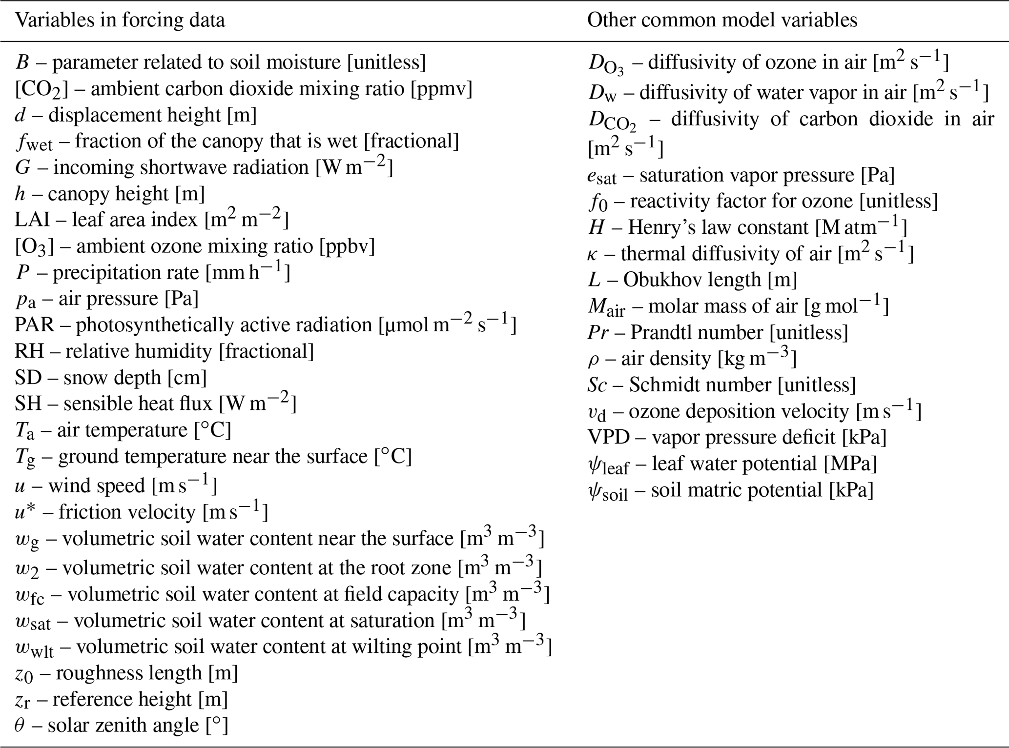
Download Print Version | Download XLSX

The forcing variables provide inputs to drive models with detailed dependencies on biophysics, such as coupled photosynthesis–stomatal conductance models, as well as models that depend mainly on atmospheric conditions. Not every model uses every forcing variable. In general, the input variables used by each single-point model should reflect the operation of the dry deposition scheme. For example, if the scheme in the host model ingests precipitation to calculate canopy wetness, rather than ingesting canopy wetness, the single-point model should ingest precipitation to calculate canopy wetness.

We note that dry deposition schemes in many chemical transport models use methods derived from classic schemes like Wesely (1989). Implementations of classic schemes may deviate from original parameterization description papers in ways that can affect simulated rates (e.g., Hardacre et al., 2015) but may not be well documented. For example, there may be changes to LULC-specific parameters or the use of different LULC categories. In addition, implementations may tie processes to variables like leaf area index to capture seasonal changes rather than relying on season-specific parameters. To foster understanding of how adaptations from original schemes influence simulated dry deposition rates, we encouraged participation in Activity 2 from models using schemes based on classic parameterizations, in addition to models with different approaches.

Like many model intercomparisons, our effort is an “ensemble of opportunity” (e.g., Galmarini et al., 2004; Tebaldi and Knutti, 2007; Potempski and Galmarini, 2009; Solazzo and Galmarini, 2015; Young et al., 2018) and may underestimate structural uncertainty due to process and parameter differences across models. Nonetheless, the design of our effort, with emphasis on processes, parameters, and sensitivities, is designed to explore uncertainty more systematically than past attempts.

The first set of Activity 2 simulations is driven by inputs from observations, and those simulations are examined here. Future work will examine sensitivity tests in which dry deposition is calculated with perturbed values of input variables (e.g., air temperature and leaf area index). We will also design tests that isolate the influence of input parameters (e.g., initial resistance to stomatal uptake and the field capacity of soil).

Diagnostic outputs required from single-point models follow the requirements of Activity 1 (see Table 4 in Galmarini et al., 2021). Among the required outputs are effective conductances (Paulot et al., 2018; Clifton et al., 2020b) for dry deposition to plant stomata, leaf cuticles, the lower canopy, and soil. (Note that not all single-point models simulate deposition to the lower canopy.) As explained and defined in Galmarini et al. (2021), an effective conductance [m s⁻¹] represents the portion of v_d that occurs via a single pathway. An effective conductance is distinct from an absolute conductance, which represents an individual process. (Note that a conductance is the inverse of a resistance.) The sum of the effective conductances across all pathways represented is v_d. In contrast, calculating v_d with absolute conductances requires considering the resistance framework. Archiving effective conductances facilitates comparison of the contribution of each pathway across dry deposition schemes with varying resistance frameworks and differing resistances to transport. Previous model comparisons examine absolute conductances and suggest that differences in pathways or processes lead to differences in v_d (Wu et al., 2018; Huang et al., 2022). Our approach with effective conductances offers a more apples-to-apples comparison across models, allowing us to definitively say whether a given pathway leads to inter-model differences in v_d.

3 Documentation of single-point models

The classic big-leaf resistance network for ozone deposition velocity (v_d) [m s⁻¹] (Table 1) is based on three resistances, which are added in series, as follows:

\begin{matrix} (1) & v_{d} = {(r_{a} + r_{b} + r_{c})}^{- 1} . \end{matrix}

Here, the variable r_a is aerodynamic resistance, r_b is quasi-laminar boundary layer resistance around the bulk surface, and r_c is surface resistance. Throughout the paper, all resistances (denoted by r) are in units of seconds per meter [s m⁻¹]. The single-point models examined here employ Eq. (1), with two exceptions. The exceptions are the Multi-layer Canopy and Chemistry Exchange Model (MLC-CHEM), which is a multilayer canopy model that simulates the ozone concentration gradient within the canopy, and the Community Multiscale Air Quality Model (CMAQ) Surface Tiled Aerosol and Gaseous Exchange (STAGE), which uses surface-specific quasi-laminar resistances. In this section, we describe methods for r_a and r_b across models (Tables S1, S2, and S3 in the Supplement) and the ozone-specific dry deposition parameters (Table S4). Equations for r_c and the v_d equation for CMAQ STAGE, which deviates from Eq. (1), are in the individual model subsections below. In the model subsection for MLC-CHEM, we describe how the model diagnoses v_d from the canopy-top ozone flux and the resistances associated with dry deposition.

With one exception (CMAQ STAGE), the single-point models use r_a equations based on Monin–Obukhov similarity theory (Table S1). However, the exact forms of the Monin–Obukhov similarity theory equations vary across the models.

Obukhov length (L) [m] (Table 1) is often used in r_a equations but is not observed. Most model L equations are similar, apart from whether models use virtual or ambient temperature and whether they include bounds on L (and what the bounds are) (Table S2).

Models are configured to accept inputs and return predicted values at the specified ozone flux measurement height at the given site (i.e., reference height z_r [m]; Table 1). Roughness length (z₀) [m] (Table 1) and displacement height (d) [m] (Table 1) are also often used in r_a equations; however, they are not observed and are especially important for estimating fluxes at z_r rather than the lowest atmospheric level of the host model. We supply estimates of z₀ and d for the models that employ them. Estimates follow Meyers et al. (1998):

\begin{matrix} (2) & z_{0} = h (0.23 - \frac{{LAI}^{0.25}}{10} - \frac{a - 1}{10}), \\ (3) & d = h (0.05 + \frac{{LAI}^{0.2}}{2} + \frac{a - 1}{20}) . \end{matrix}

Here, the variable h [m] is canopy height (Table 1), LAI [m² m⁻²] is leaf area index (Table 1), and a [unitless] is a parameter based on LULC. Meyers et al. (1998) suggest a correction for z₀ if LAI is less than 1, but we do not employ this correction given that it creates discontinuities in the time series.

Table S3 provides the quasi-laminar boundary layer resistance equations. Most models treat this resistance for the bulk surface (i.e., r_b in Eq. 1) and most use r_b from Wesely and Hicks (1977). A key part of r_b parameterizations is the ratio scaling the quasi-laminar boundary layer resistance for heat to ozone (R_diff,b) (Table S4). $R_{diff, b} = S c / P r$ , where Sc [unitless] is the Schmidt number (Table 1) and Pr [unitless] is the Prandtl number (Table 1). All but one employ $R_{diff, b} = Sc / \Pr = κ / D_{O_{3}}$ where κ [m² s⁻¹] is thermal diffusivity of air (Table 1) and $D_{O_{3}}$ [m² s⁻¹] is ozone diffusivity in air (Table 1); however, values of κ and $D_{O_{3}}$ vary across models (Table S4).

Table S4 presents model prescriptions for ozone-specific dry deposition parameters: the ratio that scales stomatal resistance from water vapor to ozone (R_diff,st), the reactivity factor for ozone (f₀) [unitless] (Table 1), and the Henry's law constant for ozone (H) [M atm⁻¹] (Table 1). Where used, values of f₀ and H are very similar across models. Some models employ temperature dependencies on H. Notably, values of R_diff,st vary from 1.2 to 1.7 across models. (The current estimate of this ratio is 1.51 according to Massman, 1998.) The Global Environmental Multiscale – Modelling Air quality and Chemistry model (GEM-MACH) Zhang and models based on GEOS-Chem are the models that prescribe lower R_diff,st values.

3.1 WRF-Chem Wesely

The Weather Research and Forecasting (WRF) model coupled with Chemistry (WRF-Chem) uses a scheme based on Wesely (1989). Parameters in Table S5 are site- and season-specific. WRF-Chem has two seasons: midsummer with lush vegetation [day of year between 90 and 270] and autumn with unharvested croplands [day of year less than 90 or greater than 270].

3.1.1 Surface resistance

Surface resistance (r_c) is calculated as follows:

\begin{matrix} (4) & r_{c} = {(\frac{1}{r_{st} + r_{m}} + \frac{1}{r_{cut}} + \frac{1}{r_{dc} + r_{c l} + r_{T}} + \frac{1}{r_{ac} + r_{g} + r_{T}})}^{- 1} . \end{matrix}

To consider the effects of air temperature (T_a) [^∘C] (Table 1), resistance r_T (Walmsley and Wesely, 1996) is calculated as follows:

\begin{matrix} (5) & r_{T} = 1000 e^{- T_{a} - 4} . \end{matrix}

In addition to the use of r_T in Eq. (4), r_T is used in the equation for cuticular resistance below.

3.1.2 Stomatal and mesophyll resistances

Stomatal resistance (r_st) is expressed as follows:

\begin{matrix} (6) & r_{st} = R_{diff, st} \frac{r_{i}}{f (T_{a}) f (G)} . \end{matrix}

The parameter r_i is initial resistance for stomatal uptake (Table S5).

The effects of T_a are calculated as follows:

\begin{matrix} (7) & f (T_{a}) = T_{a} \frac{(40 - T_{a})}{400} . \end{matrix}

The effects of incoming shortwave radiation (G) [W m⁻²] (Table 1) are expressed as follows:

\begin{matrix} (8) & f (G) = {(1 + {(\frac{200}{G + 0.1})}^{2})}^{- 1} . \end{matrix}

Mesophyll resistance (r_m) is calculated as follows:

\begin{matrix} (9) & r_{m} = {(\frac{H}{3000} + 100 f_{0})}^{- 1} . \end{matrix}

3.1.3 Cuticular resistance

Cuticular resistance (r_cut) is expressed as follows:

\begin{matrix} (10) & r_{cut} = \{\begin{cases} \frac{r_{lu} + r_{T}}{\frac{H}{10^{5}} + f_{0}}, RH \leq 0.95 and P = 0 \\ {(\frac{1}{W} + \frac{3}{r_{lu} + r_{T}})}^{- 1}, RH > 0.95 or P > 0 . \end{cases} \end{matrix}

Here, the parameter r_lu is initial resistance for cuticular uptake (Table S5), RH is relative humidity [fractional] (Table 1), and P is precipitation rate [mm h⁻¹] (Table 1). The parameter W is used to account for leaf wetness:

\begin{matrix} (11) & W = \{\begin{array}{l} 3000, P = 0 \\ 1000, P > 0 . \end{array} \end{matrix}

3.1.4 Resistances to the lower canopy and ground (and associated resistances to transport)

The resistance associated with within-canopy convection (r_dc) is calculated as follows:

\begin{matrix} (12) & r_{dc} = 100 (1 + \frac{1000}{G}) . \end{matrix}

Resistances to the lower canopy (r_cl), in-canopy turbulence (r_ac), and the ground (r_g) are prescribed (Table S5).

3.2 GEOS-Chem Wesely

GEOS-Chem is based on Wesely (1989). Wang et al. (1998) describe the initial implementation. We examine the scheme from GEOS-Chem v13.3. Parameters in Table S6 are site-specific. If there is snow, surface resistance (r_c) is calculated with the snow parameters in Table S6.

3.2.1 Surface resistance

Surface resistance (r_c) is expressed as follows:

\begin{matrix} (13) & r_{c} = {(\frac{1}{r_{st} + r_{m}} + \frac{1}{r_{cut}} + \frac{1}{r_{dc} + r_{cl}} + \frac{1}{r_{ac} + r_{g}})}^{- 1} . \end{matrix}

To consider effects of T_a, resistance r_T is calculated as follows:

\begin{matrix} (14) & r_{T} = 1000 e^{- T_{a} - 4} . \end{matrix}

The variable r_T is used in the below equations for the resistances to cuticles, the lower canopy, and the ground.

3.2.2 Stomatal and mesophyll resistances

Stomatal resistance (r_st) is expressed as follows:

\begin{matrix} (15) & r_{st} = R_{diff, st} \frac{r_{i}}{{LAI}_{eff} f (T_{a})} . \end{matrix}

Here, the parameter r_i is the initial resistance to stomatal uptake (Table S6), and LAI_eff [m² m⁻²] is the effective LAI, which is the surface area of actively transpiring leaves per ground surface area. The variable LAI_eff is calculated as a function of LAI and solar zenith angle (θ) [^∘] (Table 1), and the cloud fraction using a parameterization developed by Wang et al. (1998). In GEOS-Chem, if G is 0, LAI_eff equals 0.01. For the single-point model, we set G to 0 when θ is greater than 95^∘ so that nighttime r_st values in the single-point model are more similar to GEOS-Chem. GEOS-Chem almost never has nonzero G values at night, but measured values are frequently small and nonzero. Here, the cloud fraction is assumed to be zero.

The effects of T_a are expressed as follows:

\begin{matrix} (16) & f (T_{a}) = \{T_{a} \begin{array}{l} 0.01, T_{a} \leq 0 \\ \frac{(40 - T_{a})}{400}, 0 < T_{a} < 40 \\ 0.01, 40 \leq T_{a} . \end{array} \end{matrix}

Mesophyll resistance (r_m) is calculated as follows:

\begin{matrix} (17) & r_{m} = {(\frac{H}{3000} + 100 f_{0})}^{- 1} . \end{matrix}

3.2.3 Cuticular resistance

Cuticular resistance (r_cut) is expressed as follows:

\begin{matrix} (18) & r_{cut} = \{\begin{cases} \frac{r_{lu} + min {r_{T}, r_{lu}}}{LAI} {(\frac{H}{10^{5}} + f_{0})}^{- 1}, \frac{r_{lu} + min {r_{T}, r_{lu}}}{LAI} < 9999 \\ 10^{12}, \frac{r_{lu} + min {r_{T}, r_{lu}}}{LAI} \geq 9999 . \end{cases} \end{matrix}

The parameter r_lu is initial resistance for cuticular uptake (Table S6).

3.2.4 Resistances to the lower canopy and ground (and associated resistances to transport)

The resistance associated with in-canopy convection (r_dc) is expressed as follows:

\begin{matrix} (19) & r_{dc} = 100 (1 + \frac{1000}{G + 10}) . \end{matrix}

The resistance to surfaces in the lower canopy (r_cl) is calculated as follows:

\begin{matrix} (20) & r_{cl} = {(\frac{H}{10^{5} (r_{cl, S} + \min \{r_{T}, r_{cl, S}\})} + \frac{f_{0}}{r_{cl, O} + min \{r_{T}, r_{cl, O}\}})}^{- 1} . \end{matrix}

Here, the parameters r_cl,S and r_cl,O are initial resistances to the lower canopy (Table S6).

The resistance to turbulent transport to the ground (r_ac) is constant (Table S6).

Resistance to the ground (r_g) is expressed as follows:

\begin{matrix} (21) & r_{g} = {(\frac{H}{10^{5} (r_{g, S} + min \{r_{T}, r_{g, S}\})} + \frac{f_{0}}{r_{g, O} + min \{r_{T}, r_{g, O}\}})}^{- 1} . \end{matrix}

Here, the parameters r_g,S and r_g,O are initial resistances to uptake on the ground (Table S6).

3.3 IFS

The ECMWF Integrated Forecasting System (IFS) uses two schemes based on Wesely (1989): Météo-France's SUMO (Michou et al., 2004) (“IFS SUMO Wesely”) and GEOS-Chem 12.7.2 (“IFS GEOS-Chem Wesely”). Unless stated otherwise, the components are the same between schemes. The IFS SUMO Wesely parameters in Table S7 are site- and season-specific. Seasons are defined as follows: “transitional spring” (March, April, and May), “midsummer” (June, July, and August), “autumn” (September, October, and November), and “late autumn” (December, January, and February). Otherwise, if there is snow, the model employs the “winter, snow” parameter values. The IFS GEOS-Chem Wesely parameters in Table S8 are site-specific. If there is snow, the model employs the snow type. For snow type, only the resistance to surfaces in the lower canopy (r_cl) is defined [1000 s m⁻¹].

3.3.1 Surface resistance

Surface resistance (r_c) is expressed as follows:

\begin{matrix} (22) & r_{c} = {(\frac{1}{r_{st} + r_{m}} + \frac{1}{r_{cut}} + \frac{1}{r_{dc} + r_{cl}} + \frac{1}{r_{ac} + r_{g} + r_{T}})}^{- 1} . \end{matrix}

To consider the effects of T_a, resistance r_T is calculated as follows:

\begin{matrix} (23) & r_{T} = 1000 e^{- T_{a} - 4} . \end{matrix}

In addition to the use of r_T in Eq. (22), r_T is included in cuticular resistance equations below.

3.3.2 Stomatal and mesophyll resistances

For IFS SUMO Wesely, stomatal resistance (r_st) is expressed as follows:

\begin{matrix} (24) & r_{st} = R_{diff, st} \frac{r_{i}}{LAI f (G) f (VPD) f (w_{2})} . \end{matrix}

The parameter r_i is initial resistance to stomatal uptake (Table S7).

The effects of G are calculated as follows:

\begin{matrix} (25) & f (G) = min \{\frac{0.004 G + 0.5}{0.81 (0.004 G + 1)}, 1\} . \end{matrix}

The effects of vapor pressure deficit (VPD) [kPa] (Table 1) are expressed as follows:

\begin{matrix} (26) & f (VPD) = \{\begin{cases} e^{0.3 VPD}, forests, \\ 1, otherwise . \end{cases} \end{matrix}

The effects of root-zone soil water content (w₂) [m³ m⁻³] (Table 1) are calculated as follows:

\begin{matrix} (27) & f (w_{2}) = \{\begin{cases} 0, w_{2} < w_{wlt} \\ \frac{w_{2} - w_{wlt}}{w_{fc} - w_{wlt}}, w_{wlt} < w_{2} < w_{fc} \\ 1, w_{2} > w_{fc} . \end{cases} \end{matrix}

Here, the parameter w_wlt is the soil water content at wilting point [m³ m⁻³] (Table 1) and w_fc is the soil water content at field capacity [m³ m⁻³] (Table 1).

For IFS GEOS-Chem Wesely, stomatal resistance (r_st) is expressed as follows:

\begin{matrix} (28) & r_{st} = R_{diff, st} \frac{r_{i}}{{LAI}_{eff} f (T_{a})} . \end{matrix}

Here, the parameter r_i is initial resistance to stomatal uptake (Table S8), and LAI_eff [m² m⁻²] is the effective LAI, which is the surface area of actively transpiring leaves per ground surface area of actively transpiring leaves. The variable LAI_eff is calculated as a function of the LAI, θ, and the cloud fraction using a parameterization developed by Wang et al. (1998). In GEOS-Chem, if G is 0, LAI_eff is equal to 0.01. For the single-point model, we set G to 0 when θ is greater than 95^∘. GEOS-Chem almost never has nonzero G at night, but measured values are frequently small and nonzero. This change makes nighttime r_st values in the single-point model more similar GEOS-Chem. Here, the cloud fraction is assumed to be zero.

The effects of T_a are calculated as follows:

\begin{matrix} (29) & f (T_{a}) = T_{a} \frac{40 - T_{a}}{400} . \end{matrix}

For both configurations, mesophyll resistance (r_m) as expressed as follows:

\begin{matrix} (30) & r_{m} = {(\frac{H}{3000} + 100 f_{0})}^{- 1} . \end{matrix}

3.3.3 Cuticular resistance

For IFS SUMO Wesely,

\begin{matrix} (31) & r_{cut} = (r_{lu} + r_{T}) {(\frac{H}{10^{5}} + f_{0})}^{- 1} . \end{matrix}

The parameter r_lu is initial resistance for cuticular uptake (Table S7).

For IFS GEOS-Chem Wesely,

\begin{matrix} (32) & r_{cut} = \frac{(r_{lu} + r_{T})}{LAI} {(\frac{H}{10^{5}} + f_{0})}^{- 1} . \end{matrix}

The parameter r_lu is initial resistance to cuticular uptake (Table S8).

3.3.4 Resistances to the lower canopy and ground (and associated resistances to transport)

The resistance associated with in-canopy convection (r_dc) is expressed as follows:

\begin{matrix} (33) & r_{dc} = 100 (1 + \frac{1000}{G}) . \end{matrix}

Resistances to surfaces in the lower canopy (r_cl), in-canopy turbulence (r_ac), and ground (r_g) are prescribed (Tables S7 and S8).

3.4 GEM-MACH Wesely

Operationally, GEM-MACH uses a dry deposition scheme based on Wesely (1989) (Makar et al., 2018). Parameters defined in Table S9 are site- and sometimes season-specific. Table S10 describes how seasons are distributed as a function of month and latitude.

3.4.1 Surface resistance

Surface resistance (r_c) is calculated as follows:

\begin{matrix} (34) & r_{c} = {(\frac{1 - W}{r_{st} + r_{m}} + \frac{1}{r_{cut}} + \frac{1}{r_{dc} + r_{cl}} + \frac{1}{r_{ac} + r_{g}})}^{- 1} . \end{matrix}

The parameter W [fractional] is used to account for leaf wetness:

\begin{matrix} (35) & W = \{\begin{cases} 0.5, P > 1 mm h^{- 1} or RH > 0.95 \\ 0, otherwise . \end{cases} \end{matrix}

3.4.2 Stomatal resistance and mesophyll resistance

Stomatal resistance (r_st) is based on Jarvis (1976), Zhang et al. (2002a, 2003), and Baldocchi et al. (1987):

\begin{matrix} (36) & r_{st} = R_{diff, st} \frac{r_{i}}{LAI max \{f (G) f (VPD) f (T_{a}) f (c_{a}), 0.0001\}} . \end{matrix}

Here, the parameter r_i is initial resistance to stomatal uptake (Table S9).

Curve-fitting of data from Jarvis (1976) and Ellsworth and Reich (1993) was used to infer the following:

\begin{matrix} (37) & f (G) = \max {0.206 \ln (G) - 0.605, 0} . \end{matrix}

The effects of VPD are expressed as follows:

\begin{matrix} (38) & \begin{aligned} f & (VPD) = \max \{0.0, max \{1.0, \\ (1.0 - 0.03 (1 - RH) 10^{\frac{0.7859 + 0.03477 T_{a}}{1 + 0.00412 T_{a}}})\}\} . \end{aligned} \end{matrix}

The effects of T_a are calculated as follows:

\begin{matrix} (39) & f (T_{a}) = {(\frac{(T_{a} - T_{\min}) (T_{\max} - T_{a})}{(T_{opt} - T_{\min}) (T_{\max} - T_{opt})})}^{0.62} . \end{matrix}

Here, the parameters T_min, T_max, and T_opt [^∘C] are the minimum, maximum, and optimum temperatures, respectively (Table S9).

The effects of the ambient carbon dioxide mixing ratio ([CO₂]) [ppmv] (Table 1) are expressed as follows:

\begin{matrix} (40) & f (c_{a}) = \{\begin{cases} 1, [{CO}_{2}] \leq 100 \\ 1 - (7.35 \times 10^{- 4} \ln (\ln (G)) - 8.75 \\ \times 10^{- 4}) [{CO}_{2}], 100 < [{CO}_{2}] < 1000 \\ 0, [{CO}_{2}] \geq 1000 . \end{cases} \end{matrix}

Mesophyll resistance (r_m) is calculated as follows:

\begin{matrix} (41) & r_{m} = {(LAI (\frac{H}{3000} + 100 f_{0}))}^{- 1} . \end{matrix}

3.4.3 Cuticular resistance

Cuticular resistance (r_cut) is expressed as follows:

\begin{matrix} (42) & r_{cut} = \frac{r_{lu}}{LAI} {(\frac{H}{10^{5}} + f_{0})}^{- 1} . \end{matrix}

The parameter r_lu is initial resistance to cuticular uptake (Table S9).

3.4.4 Resistances to the lower canopy and ground (and associated resistances to transport)

The resistance associated with in-canopy convection (r_dc) is calculated as follows:

\begin{matrix} (43) & r_{dc} = 100 + (1 + \frac{1000}{G + 10}) . \end{matrix}

The resistance posed by uptake to the lower canopy (r_cl) is expressed as follows:

\begin{matrix} (44) & r_{cl} = {(\frac{H}{10^{5} r_{cl, S}} + \frac{f_{0}}{r_{cl, O}})}^{- 1} . \end{matrix}

Here, the parameters r_cl,S and r_cl,O are initial resistances to uptake by surfaces in the lower canopy (Table S9).

The parameter r_ac is resistance to in-canopy turbulence and r_g is resistance to the ground; both are prescribed (Table S9).

3.5 GEM-MACH Zhang

GEM-MACH also has an implementation of Zhang et al. (2002b). Parameters in Table S11 are site-specific.

3.5.1 Surface resistance

Surface resistance (r_c) is expressed as follows:

\begin{matrix} (45) & r_{c} = min \{10, {(\frac{1 - W}{r_{st}} + \frac{1}{r_{cut}} + \frac{1}{r_{ac} + r_{g}})}^{- 1}\} . \end{matrix}

The variable W [fractional] is used to account for leaf wetness:

\begin{matrix} (46) & W = \{\begin{cases} \min \{0.5, \frac{G - 200}{800}\}, precipitation or dew, \\ T_{a} > 1, G > 200 \\ 0, otherwise . \end{cases} \end{matrix}

Precipitation is assumed to occur if P is greater than 0.20 mm h⁻¹. Dew is assumed to occur if P is less than 0.20 mm h⁻¹ and

\begin{matrix} (47) & u^{*} < c_{dew} \frac{1.5}{\max \{1 \times 10^{- 4}, \frac{0.622 e_{sat} (1 - RH)}{p_{a}}\}} . \end{matrix}

Here, the variable e_sat [Pa] is saturation vapor pressure (Table 1), p_a [Pa] is air pressure (Table 1), and c_dew is the dew coefficient [0.3].

3.5.2 Stomatal resistance

Stomatal resistance (r_st) is expressed as follows:

\begin{matrix} (48) & r_{st} = R_{diff, st} \frac{r_{i} (LAI, PAR)}{f (T_{a}) f (VPD) f (ψ_{leaf})} . \end{matrix}

Here, the variable r_i (LAI, PAR) is initial resistance to stomatal uptake that varies with LAI and PAR, based on Norman (1982) and Zhang et al. (2001):

\begin{matrix} (49) & r_{i} (LAI, PAR) = {(\frac{{LAI}_{sun}}{r_{i} (1 + \frac{b_{rs}}{{PAR}_{sun}})} + \frac{{LAI}_{shd}}{r_{i} (1 + \frac{b_{rs}}{{PAR}_{shd}})})}^{- 1} . \end{matrix}

The parameter r_i is initial resistance to stomatal uptake (Table S11), b_rs [W m⁻²] is empirical (Table S11), and LAI_sun and LAI_shd [m² m⁻²] are sunlit and shaded LAI, respectively. The latter two parameters are calculated as follows:

\begin{matrix} (50) & {LAI}_{sun} = \frac{1 - e^{- K_{b} LAI}}{K_{b}}, \\ (51) & {LAI}_{shd} = LAI - {LAI}_{sun} . \end{matrix}

The variable K_b is the canopy light extinction coefficient [unitless]:

\begin{matrix} (52) & K_{b} = \frac{0.5}{\cos (\frac{π}{180} θ)} . \end{matrix}

The variables PAR_sun and PAR_shd [W m⁻²] are photosynthetically active radiation reaching sunlit and shaded leaves, respectively:

\begin{matrix} (53) & \begin{aligned} {PAR}_{shd} & = {PAR}_{diff} e^{- 0.5 {LAI}^{a}} \\ + 0.07 {PAR}_{dir} (1 - 0.1 LAI) e^{- \cos (\frac{π}{180} θ),} \end{aligned} \\ (54) & {PAR}_{sun} = {PAR}_{shd} + \frac{0.5 {PAR}_{dir}^{b}}{\cos (\frac{π}{180} θ) .} \end{matrix}

If LAI is greater than 2.5 m² m⁻² and G is less than 200 W m⁻², the empirical parameter a equals 0.8 and b equals 0.8. Otherwise, a equals 0.07 and b equals 1. The calculation of direct and diffuse components of PAR (PAR_dir and PAR_diff, respectively) has been updated from Zhang et al. (2001) to follow Iqbal (1983):

\begin{matrix} (55) & {PAR}_{dir} = G {FRAD}_{V} {FD}_{V}, \\ (56) & {PAR}_{diff} = G {FRAD}_{V} (1 - {FD}_{V}) . \end{matrix}

The variable FRAD_V is calculated as follows:

\begin{matrix} (57) & {FRAD}_{V} = \frac{R_{V}}{R_{V} + R_{N}} . \end{matrix}

The variables R_V and R_N are expressed as follows:

\begin{matrix} (58) & R_{N} = {RD}_{M} + {RD}_{N}, \\ (59) & R_{V} = {RD}_{U} + {RD}_{V} . \end{matrix}

The variable RD_U is calculated as follows:

\begin{matrix} (60) & {RD}_{U} = 600 \cos (\frac{π}{180} θ) e^{\frac{- 0.185 p_{a}}{p_{std} \cos (\frac{π}{180} θ)}} . \end{matrix}

The variable p_std is standard air pressure [1.0132×10⁵ Pa].

The variable RD_V is expressed as follows:

\begin{matrix} (61) & {RD}_{V} = 0.42 (600 - {RD}_{U}) \cos (\frac{π}{180} θ) . \end{matrix}

The variable RD_M is calculated as follows:

\begin{matrix} (62) & \begin{aligned} {RD}_{M} & = \cos (\frac{π}{180} θ) (720 e^{(- \frac{0.06 p_{a}}{p_{std} \cos (\frac{π}{180} θ)})} \\ - (1320 \cdot 0.077 {(\frac{2 p_{a}}{p_{std} \cos (\frac{π}{180} θ)})}^{0.3})) . \end{aligned} \end{matrix}

The variable RD_N is expressed as follows:

\begin{matrix} (63) & \begin{aligned} {RD}_{N} & = 0.65 \cos (\frac{π}{180} θ) (720 \\ - {RD}_{M} - (1320 \cdot 0.077 {(\frac{2 p_{a}}{p_{std} \cos (\frac{π}{180} θ)})}^{0.3})) . \end{aligned} \end{matrix}

The variable FD_V is calculated as follows:

\begin{matrix} (64) & {FD}_{V} = \{\begin{cases} 0.941124 {RD}_{U} / R_{V}, & \frac{G}{R_{V} + R_{N}} \geq 0.89 \\ (1 - {(\frac{(0.9 - \frac{G}{R_{V} + R_{N}})}{0.7})}^{\frac{2}{3}}) {RD}_{U} / R_{V}, & 0.21 \geq \frac{G}{R_{V} + R_{N}} < 0.89 \\ 0.00955 {RD}_{U} / R_{V}, & \frac{G}{R_{V} + R_{N}} < 0.21 . \end{cases} \end{matrix}

The effects of T_a are as follows:

\begin{matrix} (65) & f (T_{a}) = (\frac{T_{a} - T_{\min}}{T_{opt} - T_{\min}}) {(\frac{T_{\max} - T_{a}}{T_{\max} - T_{opt}})}^{\frac{T_{\max} - T_{opt}}{T_{\max} - T_{\min}}} . \end{matrix}

Here, the parameters T_min, T_max, and T_opt [^∘C] are the minimum, maximum, and optimum temperatures, respectively (Table S11).

The effects of VPD are expressed as follows:

\begin{matrix} (66) & f (VPD) = \min \{\max \{1 - b_{vpd} VPD, 0\}, 1\} . \end{matrix}

The parameter b_vpd [kPa⁻¹] is empirical (Table S11).

The effects of the leaf water potential (ψ_leaf) [MPa] (Table 1) are calculated as follows:

\begin{matrix} (67) & f (ψ_{leaf}) = \min \{\max \{\frac{ψ_{leaf} - ψ_{leaf, 2}}{ψ_{leaf, 1} - ψ_{leaf, 2}}, 0\}, 1\} . \end{matrix}

The variable ψ_leaf is approximated as follows:

\begin{matrix} (68) & ψ_{leaf} = - 0.72 - 0.0013 G . \end{matrix}

The parameters ψ_leaf,1 and ψ_leaf,2 [MPa] are empirical (Table S11).

3.5.3 Cuticular resistance

Cuticular resistance (r_cut) is expressed as follows:

\begin{matrix} (69) & r_{cut} = \{\begin{cases} \max \{100, \frac{c_{cut, dry}}{u^{*} {LAI}^{0.25} e^{3 RH}}\}, T_{a} \geq - 1, neither precipitation nor dew \\ \frac{c_{cut, wet}}{u^{*} \sqrt{LAI}}, T_{a} \geq - 1, precipitation or dew occurring \\ \max \{100, \frac{C_{cut, dry}}{u^{*} {LAI}^{0.25} e^{3 RH}} \min \{2, e^{0.2 (- 1 - T_{a})}\}\}, T_{a} < - 1 . \end{cases} \end{matrix}

The variable u^* [m s⁻¹] is friction velocity (Table 1) and c_cut,dry [unitless] is a coefficient related to dry cuticular uptake (Table S11).

If the fraction of snow coverage (f_snow) is greater than 10⁻⁴, a correction is applied:

\begin{matrix} (70) & r_{cut} = {(\frac{1 - f_{snow}}{r_{cut}} + \frac{f_{snow}}{2000})}^{- 1} . \end{matrix}

If LAI is less than $2 \times 10^{- 6}$ m² m⁻², r_cut is very large.

The fraction of snow coverage (f_snow) is calculated as follows:

\begin{matrix} (71) & f_{snow} = \min \{1, \frac{SD}{{SD}_{\max}}\} . \end{matrix}

The variable SD [cm] is snow depth (Table 1) and SD_max [cm] is maximum snow depth (Table S11).

3.5.4 Resistance to the ground (and associated resistance to transport)

The resistance to in-canopy turbulence (r_ac) is expressed as follows:

\begin{matrix} (72) & r_{ac} = r_{ac 0} \frac{{LAI}^{0.25}}{{(u^{*})}^{2}} . \end{matrix}

The variable r_ac0 is calculated as follows:

\begin{matrix} (73) & r_{ac 0} = r_{ac 0, \min} + \frac{LAI - {LAI}_{\min}}{{LAI}_{\max} - {LAI}_{\min}} (r_{ac 0, \max} - r_{ac 0, \min}) . \end{matrix}

Here, the parameters LAI_min and LAI_max [m² m⁻²] are the minimum and maximum LAI values across the site's observational record, respectively, and r_ac0,min and r_ac0,max are initial resistances (Table S11).

Ground resistance (r_g) is prescribed but modified under certain conditions. If T_s is less than −1 ^∘C,

\begin{matrix} (74) & r_{g} = r_{g} \min \{2, e^{- 0.2 (T_{s} + 1)}\} . \end{matrix}

The near-surface air temperature (T_s) is approximated from a linear interpolation between T_a and T_g to a height of 1.5 m.

If f_snow (see Eq. 71) is greater than or equal to 10⁻⁴,

\begin{matrix} (75) & r_{g} = {(\frac{1 - min \{1, 2 f_{snow}\}}{r_{g}} + \frac{min \{1, 2 f_{snow}\}}{2000})}^{- 1} . \end{matrix}

3.6 CMAQ M3Dry

M3Dry (Pleim and Ran, 2011) is designed to couple with the Pleim–Xiu land surface model (PX LSM; Pleim and Xiu, 1995) in the Weather Research and Forecasting (WRF) model and is used operationally in CMAQ. There is also M3Dry-psn, which follows M3Dry but uses a coupled photosynthesis–stomatal conductance model. M3Dry-psn was developed and evaluated with the intention to supplement PX LSM and M3Dry in CMAQ (Ran et al., 2017). To date, however, M3Dry-psn has not been implemented in CMAQ. The parameters in Table S12 are site-specific.

3.6.1 Surface resistance

Surface resistance (r_c) is expressed as follows:

\begin{matrix} (76) & r_{c} = {(\begin{array}{l} f_{veg} (\frac{1}{r_{st} + r_{m}} + \frac{(1 - f_{wet}) LAI}{r_{cut, dry}} + \frac{f_{wet} L A I}{r_{cut, wet}} + \frac{1}{r_{ac} + r_{g}}) \\ + \frac{1 - f_{veg}}{r_{g}} \end{array})}^{- 1} . \end{matrix}

Here, the parameter f_veg is the fraction of the site covered by the vegetation canopy (Table S12) and f_wet is the fraction of canopy that is wet (Table 1).

3.6.2 Stomatal and mesophyll resistances

For M3Dry, stomatal resistance (r_st) follows Xiu and Pleim (2001):

\begin{matrix} (77) & r_{st} = R_{diff, st} \frac{r_{i}}{LAI f (PAR) f (w_{2}) f ({RH}_{l}) f (T_{a})} . \end{matrix}

The parameter r_i is initial resistance to stomatal uptake (Table S12).

The effects of photosynthetically active radiation (PAR) [µmol m⁻² s⁻¹] (Table 1) follow Echer and Rosolem (2015):

\begin{matrix} (78) & f (PAR) = (1 - a LAI) (1 - e^{- 0.0017 PAR}) . \end{matrix}

The parameter a [unitless] is empirical (Table S12).

The effects of w₂ follow Xiu and Pleim (2001):

\begin{matrix} (79) & f (w_{2}) = {(1 + e^{- 5 (\frac{w_{2} - w_{wlt}}{w_{fc} - w_{wlt}} - (\frac{w_{fc} - w_{wlt}}{3} + w_{wlt}))})}^{- 1} . \end{matrix}

The effects of leaf-level RH (RH_l) [fractional] are expressed as follows:

\begin{matrix} (80) & f ({RH}_{l}) = {RH}_{l} = \frac{q_{a} {(r_{a} + r_{b, v})}^{- 1} + q_{s} r_{st, v}^{- 1}}{(r_{st, v}^{- 1} + {(r_{a} + r_{b, v})}^{- 1}) q_{s}} . \end{matrix}

Here, the variable q_a is the ambient air humidity mixing ratio, q_s is the saturation mixing ratio at leaf temperature (T_leaf), r_b,v is the quasi-laminar boundary layer resistance for water vapor, and r_st,v is the stomatal resistance for water vapor. M3Dry assumes that, when the sensible heat flux (SH) [W m⁻²] (Table 1) is greater than zero, the T_leaf equals $T_{a} - \frac{SH}{(r_{a} + r_{b, h}) ρ c_{p}}$ , where r_b,h is quasi-laminar boundary layer resistance for heat. Otherwise, T_leaf equals T_a. Equation (80) is computed using an implicit quadratic solution as described by Xiu and Pleim (2001).

The effects of T_a are expressed as follows:

\begin{matrix} (81) & f (T_{a}) = \{\begin{cases} {(1 + e^{- 0.41 (T_{a} - 8.9)})}^{- 1}, T_{a} \leq 29 \\ {(1 + e^{0.5 (T_{a} - 40.85)})}^{- 1}, T_{a} > 29 . \end{cases} \end{matrix}

For M3Dry-psn, r_st is simulated at the leaf level using the Ball–Woodrow–Berry approach (Ball et al., 1987), as described by Collatz et al. (1991, 1992) and Bonan et al. (2011):

\begin{matrix} (82) & r_{st} = {(g_{0} + g_{1} \frac{A_{n}}{\frac{p_{{CO}_{2}, l}}{p_{a}}} {RH}_{l})}^{- 1} \frac{D_{{CO}_{2}}}{D_{O_{3}}} \frac{1000.0 ρ}{M_{air}} . \end{matrix}

Here, the parameter g₀ equals 0.01 mol CO₂ m⁻² s⁻¹ for C₃ plants; g₁ equals 9 [unitless]; A_n is the leaf-level net photosynthesis [mol CO₂ m⁻² s⁻¹]; $p_{{CO}_{2}, l}$ is the carbon dioxide partial pressure at the leaf surface [Pa]; RH_l is the leaf-level RH [fractional], which follows Eq. (80) as described for M3Dry; $D_{{CO}_{2}}$ [m² s⁻¹] is the carbon dioxide diffusivity in air (Table 1); ρ [kg m⁻³] is the air density (Table 1); and M_air [g mol⁻¹] is the molar mass of air (Table 1). Leaf-level A_n is estimated based on Farquhar et al. (1980) as described by Ran et al. (2017), based on co-limitation among three potential assimilation rates, limited by Rubisco, light, and transport of photosynthetic products. The maximum rate of the carboxylation of Rubisco (V_cmax) [µmol m² s⁻¹] is key for A_n; thus, we include values at 25 ^∘C in Table S12.

Leaf-level A_n and r_st are calculated separately for sunlit versus shaded leaves in M3Dry-psn. Sunlit and shaded portions of the LAI (LAI_sun and LAI_shd, respectively) follow Campbell and Norman (1998) and Song et al. (2009). Canopy-scale r_st is expressed as follows:

\begin{matrix} (83) & r_{st} = {((\frac{{LAI}_{sun}}{r_{st, sun}} + \frac{{LAI}_{shd}}{r_{st, shd}}) f (w_{2}))}^{- 1} . \end{matrix}

The variables r_st,sun and r_st,shd are leaf-level stomatal resistances for sunlit and shaded leaves, respectively, calculated via Eq. (82). The function f(w₂) follows Eq. (79).

For both M3Dry and M3Dry-psn, mesophyll resistance (r_m) is expressed as follows:

\begin{matrix} (84) & r_{m} = \frac{0.01}{LAI} . \end{matrix}

3.6.3 Cuticular resistances

The variable r_cut,wet is the resistance to wet cuticles:

\begin{matrix} (85) & r_{cut, wet} = \{\begin{cases} 1250, T_{g} > 0 \\ 6667, T_{g} < 0 . \end{cases} \end{matrix}

The variable T_g [^∘C] is ground temperature near the surface (Table 1).

The variable r_cut,dry is resistance to dry cuticles:

\begin{matrix} (86) & r_{cut, dry} = r_{cut, dry, 0} (1 - f (RH)) + r_{cut, wet} f (RH) . \end{matrix}

The parameter $r_{cut, dry, 0}$ equals 2000 s m⁻¹.

The effects of RH are expressed as follows:

\begin{matrix} (87) & f (RH) = max \{100 \frac{RH - 0.7}{0.3}, 0\} . \end{matrix}

3.6.4 Resistance to the ground (and associated resistance to transport)

The resistance to in-canopy turbulence (r_ac) follows Erisman et al. (1994):

\begin{matrix} (88) & r_{ac} = 14 \frac{h LAI}{u_{*}} . \end{matrix}

Ground resistance (r_g) is calculated as follows:

\begin{matrix} (89) & r_{g} = \{\begin{cases} {(\frac{1 - f_{wet}}{r_{g, dry}} + \frac{f_{wet}}{r_{g, wet}})}^{- 1}, no snow, \\ {(\frac{1 - X_{m}}{r_{snow}} + \frac{X_{m}}{r_{sndiff} + r_{g, wet}})}^{- 1}, snow . \end{cases} \end{matrix}

The variable r_g,wet is expressed as

\begin{matrix} (90) & r_{g, wet} = \{\begin{cases} 500, T_{g} > 0 \\ 6667, T_{g} < 0 . \end{cases} \end{matrix}

The variable r_g,dry is expressed as follows (Massman, 2004; Mészáros et al., 2009):

\begin{matrix} (91) & r_{g, dry} = 200 + (r_{g, wet} - 200) \frac{w_{g}}{w_{fc}} . \end{matrix}

If the near-surface soil water content (w_g) [m³ m⁻³] (Table 1) is greater than w_fc, the soil is wet (i.e., r_g,dry equals r_g,wet). The parameter r_snow is resistance to snow or ice [6667 s m⁻¹] and r_sndiff is resistance to diffusion through the snowpack [10 s m⁻¹]. Parallel pathways to frozen snow/ice and diffusion through the snowpack to liquid water follow Bales et al. (1987). Snow liquid water mass (X_m) is calculated as follows:

\begin{matrix} (92) & X_{m} = \{\begin{cases} max \{0.02 {(T_{a} + 1)}^{2}, 0.5\}, T_{a} > - 1 \\ 0, T_{a} < - 1 . \end{cases} \end{matrix}

3.7 CMAQ STAGE

The Surface Tiled Aerosol and Gaseous Exchange (STAGE) parameterization is an option in CMAQ. Parameters in Table S13 are site-specific.

3.7.1 Deposition velocity

The ozone deposition velocity (v_d) follows:

\begin{matrix} (93) & \begin{aligned} v_{d} & = f_{veg} {(r_{a} + \frac{1}{\frac{1}{r_{b, v} + \frac{1}{\frac{1}{r_{st} + r_{m}} + \frac{1}{r_{cut}}}} + \frac{1}{r_{ac} + r_{b, g} + r_{g}}})}^{- 1} \\ + (1 - f_{veg}) {(r_{a} + r_{b, g} + r_{g})}^{- 1} \end{aligned} \end{matrix}

CMAQ STAGE considers separate quasi-laminar boundary layer resistances around vegetation versus the ground (r_b,v and r_b,g, respectively) (Table S3). The parameter f_veg is the vegetated fraction of the site; the M3Dry value is used (Table S12).

3.7.2 Stomatal and mesophyll resistances

Stomatal resistance (r_st) follows Pleim and Ran (2011):

\begin{matrix} (94) & r_{st} = R_{diff, st} \frac{r_{i}}{LAI f (PAR) f (w_{2}) f ({RH}_{l}) f (T_{a})} . \end{matrix}

The parameter r_i is initial resistance to stomatal uptake (Table S13). The functions follow M3Dry (Eqs. 78–81).

Mesophyll resistance (r_m) follows Wesely (1989):

\begin{matrix} (95) & r_{m} = {(\frac{H}{3000} + 100 f_{0})}^{- 1} . \end{matrix}

3.7.3 Cuticular resistance

Cuticular resistance (r_cut) is expressed as follows:

\begin{matrix} (96) & r_{cut} = {(LAI (\frac{f_{wet}}{1250} + \frac{1 - f_{wet}}{2000}))}^{- 1} . \end{matrix}

3.7.4 Resistance to the ground (and associated resistance to transport)

The resistance to in-canopy turbulence (r_ac) is similar to Shuttleworth and Wallace (1985):

\begin{matrix} (97) & r_{ac} = \int_{0}^{h} \frac{d z}{K_{t}} . \end{matrix}

The variable K_t is in-canopy eddy diffusivity [m² s⁻¹]. By applying the drag coefficient ( $C_{d} = \frac{u_{*}^{2}}{u^{2}}$ ), assuming a uniform vertical distribution of leaves, and using an in-canopy attenuation coefficient of momentum following Yi (2008) $[\frac{LAI}{2}]$ , we obtain the following:

\begin{matrix} (98) & r_{ac} = \Pr \frac{u}{u_{*}^{2}} (e^{\frac{LAI}{2}} - 1) = r_{a} (e^{\frac{LAI}{2}} - 1) . \end{matrix}

The variable u [m s⁻¹] is wind speed (Table 1).

The resistance to the ground (r_g) changes whether the ground is snow-covered, dry, or wet (wet is w_g greater than or equal to w_sat, where w_sat [m³ m⁻³] is soil water content at saturation; Table 1). For dry ground, r_g follows Fares et al. (2014) and Fumagalli et al. (2016). An asymptotic function bounds the resistance, following observations reported in Fumagalli et al. (2016):

\begin{matrix} (99) & r_{g} = \{\begin{cases} 250 + 2000 atan (\frac{{(\frac{w_{g} - w_{wlt}}{w_{fc}})}^{B}}{π}), w < w_{sat} \\ \frac{62 500}{H R (T_{g} + 273.15)}, w \geq w_{sat} \\ \frac{1 - X_{m}}{r_{snow}} + \frac{X_{m}}{r_{sndiff} + \frac{62 500}{H R (T_{g} + 273.15)}}, snow . \end{cases} \end{matrix}

Here, the parameter R [L atm K⁻¹ mol⁻¹] is the universal gas constant, B [unitless] is an empirical parameter related to soil moisture (Table 1), r_snow is resistance to snow or ice [6667 s m⁻¹], and r_sndiff is resistance to diffusion through the snowpack [10 s m⁻¹]. The liquid fraction of the quasi-liquid layer in snow (X_m) is modeled as a system dominated by van der Waals forces using the temperature parameterization following Huthwelker et al. (2006) and assuming a maximum of 20 % to match gas–liquid partitioning findings in Conklin et al. (1993):

\begin{matrix} (100) & X_{m} = \{\begin{array}{cc} \frac{0.025}{{(273.15 - T_{g})}^{1 / 3}}, & 0.002 < 273.15 - T_{g} < 10 \\ 0.2, & 273.15 - T_{g} < 0.002 . \end{array} \end{matrix}

3.8 TEMIR

The Terrestrial Ecosystem Model in R (TEMIR) (Tai et al., 2023) provides two dry deposition schemes (Sun et al., 2022): Wesely and Zhang. Wesely in TEMIR largely follows GEOS-Chem version 12.0.0, while Zhang follows Zhang et al. (2003). In both schemes, the default stomatal resistance is highly empirical. TEMIR can also use two photosynthesis-based stomatal conductance models (hereinafter, “psn”): the Farquhar–Ball–Berry model (hereinafter, “BB”; Farquhar et al., 1980; Ball et al., 1987) and the Medlyn et al. (2011) model (hereinafter, “Medlyn”). Thus, three stomatal conductance models are used for TEMIR Wesely and TEMIR Zhang, respectively. TEMIR Zhang parameters in Table S14 and TEMIR psn parameters in Table S15 are site-specific.

3.8.1 Surface resistance

For Wesely, surface resistance (r_c) is calculated as follows:

\begin{matrix} (101) & r_{c} = {(\frac{1}{r_{st}} + \frac{1}{r_{cut}} + \frac{1}{r_{dc} + r_{cl}} + \frac{1}{r_{ac} + r_{g}})}^{- 1} . \end{matrix}

For Zhang, surface resistance (r_c) is expressed as follows:

\begin{matrix} (102) & r_{c} = {(\frac{1 - W}{r_{st}} + \frac{1}{r_{cut}} + \frac{1}{r_{ac} + r_{g}})}^{- 1} . \end{matrix}

The parameter W [fractional] is used to account for leaf wetness. If P is greater than 0.2 mm h⁻¹,

\begin{matrix} (103) & W = \{\begin{cases} 0, G \leq 200 \\ \frac{G - 200}{800}, 200 \leq G \leq 600 \\ 0.5, G > 600 . \end{cases} \end{matrix}

3.8.2 Stomatal resistance

For Wesely, stomatal resistance (r_st) is expressed as follows:

\begin{matrix} (104) & r_{st} = R_{diff, st} \frac{r_{i}}{{LAI}_{eff} f (T_{a})} . \end{matrix}

Here, the parameter r_i is initial resistance to stomatal uptake (same for GEOS-Chem Wesely; Table S6), and LAI_eff [m² m⁻²] is the effective LAI, which is the surface area of actively transpiring leaves per ground surface area. The variable LAI_eff is calculated as a function of the LAI, θ, and the cloud fraction using a parameterization developed by Wang et al. (1998). In GEOS-Chem, if G is 0, LAI_eff equals 0.01. For the single-point model, we set G to 0 when θ is greater than 95^∘ so that nighttime r_st values in the single-point model are more similar GEOS-Chem. GEOS-Chem almost never has nonzero G at night, but measured values are frequently small and nonzero. Here, the cloud fraction is assumed to be zero.

The effects of T_a are expressed as follows:

\begin{matrix} (105) & f (T_{a}) = \{T_{a} \begin{array}{l} 0.01, T_{a} \leq 0 \\ \frac{(40 - T_{a})}{400}, 0 < T_{a} < 40 \\ 0.01, 40 \leq T_{a} . \end{array} \end{matrix}

For Zhang, stomatal resistance (r_st) is calculated as follows:

\begin{matrix} (106) & r_{st} = R_{diff, st} \frac{r_{i} (LAI, PAR)}{f (T_{a}) f (VPD) f (ψ_{leaf}) .} \end{matrix}

Dependencies on T_a, VPD, and ψ_leaf are as described in Brook et al. (1999).

The variable r_i (LAI, PAR) is expressed as follows:

\begin{matrix} (107) & r_{i} (LAI, PAR) = {(\frac{{LAI}_{sun}}{r_{i} (1 + \frac{b_{rs}}{{PAR}_{sun}})} + \frac{{LAI}_{shd}}{r_{i} (1 + \frac{b_{rs}}{{PAR}_{shd}})})}^{- 1} . \end{matrix}

Here, the parameter r_i is the initial resistance to stomatal uptake (Table S14), b_rs [W m⁻²] is empirical (Table S14), and LAI_sun and LAI_shd [m² m⁻²] are sunlit and shaded LAI, respectively. The latter two parameters are expressed as follows:

\begin{matrix} (108) & {LAI}_{sun} = \frac{1 - e^{- K_{b} LAI}}{K_{b}}, \\ (109) & {LAI}_{shd} = LAI - {LAI}_{sun} . \end{matrix}

The variable K_b is the canopy light extinction coefficient [unitless]:

\begin{matrix} (110) & K_{b} = \frac{0.5}{\cos (\frac{π}{180} θ)} . \end{matrix}

The variables PAR_sun and PAR_shd [W m⁻²] are PAR reaching sunlit and shaded leaves, respectively:

\begin{matrix} (111) & \begin{aligned} {PAR}_{shd} & = R_{diff} e^{- 0.5 {LAI}^{a}} \\ + 0.07 R_{dir} (1.1 - 0.1 LAI) e^{- \cos (\frac{π}{180} θ),} \end{aligned} \\ (112) & {PAR}_{sun} = {PAR}_{shd} + \frac{R_{dir}^{b} \cos (\frac{π}{180} α)}{\cos (\frac{π}{180} θ) .} \end{matrix}

Here, the parameter α is the angle between the leaf and the sun [60^∘], and R_diff and R_dir are downward visible radiation fluxes from diffuse and direct-beam radiation above the canopy, respectively. We use the diffuse fraction from the Modern-Era Retrospective analysis for Research and Applications, Version 2 (MERRA-2) reanalysis product (GMAO, 2015) to separate R_diff and R_dir from observed PAR. If the LAI is less than 2.5 m² m⁻² or G is less than 200 W m⁻², a equals 0.7 and b equals 1. Otherwise, a equals 0.8 and b equals 0.8.

The effects of T_a are expressed as follows:

\begin{matrix} (113) & f (T_{a}) = (\frac{T_{a} - T_{\min}}{T_{opt} - T_{\min}}) {(\frac{T_{\max} - T_{a}}{T_{\max} - T_{opt}})}^{\frac{T_{\max} - T_{opt}}{T_{opt} - T_{\min}}} . \end{matrix}

The parameters T_min, T_max, and T_opt [^∘C] are the minimum, maximum, and optimum temperatures, respectively (Table S14).

The effects of VPD are expressed as follows:

\begin{matrix} (114) & f (VPD) = 1 - b_{VPD} VPD . \end{matrix}

The parameter b_VPD [kPa⁻¹] is empirical (Table S14).

The effects of ψ_leaf are calculated as follows:

\begin{matrix} (115) & f (ψ_{leaf}) = \frac{ψ_{leaf} - ψ_{leaf, 2}}{ψ_{leaf, 1} - ψ_{leaf, 2}} . \end{matrix}

The parameters ψ_leaf,1 and ψ_leaf,2 [MPa] are empirical (Table S14), whereas ψ_leaf is parameterized as follows:

\begin{matrix} (116) & ψ_{leaf} = - 0.72 - 0.0013 G . \end{matrix}

We now describe psn options for TEMIR Wesely and TEMIR Zhang. For BB (Ball et al., 1987; Farquhar et al., 1980; von Caemmerer and Farquhar, 1981; Collatz et al., 1991, 1992),

\begin{matrix} (117) & r_{st} = {(β_{t} g_{0} + g_{1} \frac{A_{n} RH}{\frac{p_{{CO}_{2}, l}}{p_{a}}})}^{- 1} \frac{p_{a}}{R θ_{a}} . \end{matrix}

Here, the parameter g₀ equals 0.01 mol m⁻² s⁻¹, g₁ equals 9, A_n is net photosynthesis [mol m⁻² s⁻¹], β_t is a soil water stress factor [unitless], $p_{{CO}_{2}, l}$ is the carbon dioxide partial pressure at the leaf surface [Pa], R is the universal gas constant [J mol⁻¹ K⁻¹], and θ_a is potential air temperature [K].

For Medlyn (Medlyn et al., 2011),

\begin{matrix} (118) & r_{st} = {(β_{t} g_{0} + \frac{D_{w}}{D_{{CO}_{2}}} (1 + \frac{g_{1 M}}{\sqrt{VPD}}) \frac{A_{n}}{\frac{p_{{CO}_{2, l}}}{p_{a}}})}^{- 1} \frac{p_{a}}{R θ_{a}} . \end{matrix}

Here, the parameter g_1M [kPa^0.5] is empirical (Table S15), g₀ equals 0.0001 mol m⁻² s⁻¹, D_w [m² s⁻¹] is the diffusivity of water vapor in air (Table 1), and the ratio of diffusivities is 1.6.

A single-layer bulk soil formulation considering the root zone (0–100 cm) is used to calculate β_t:

\begin{matrix} (119) & β_{t} = \{\begin{cases} 1, ψ_{soil} > ψ_{soil, fc} \\ \frac{ψ_{soil, wlt} - ψ_{soil}}{ψ_{soil, wlt} - ψ_{soil, fc}}, ψ_{soil, wlt} \leq ψ_{soil} \leq ψ_{soil, fc} \\ 0, ψ_{soil} < ψ_{soil, fc} . \end{cases} \end{matrix}

The variable ψ_soil [kPa] is soil matric potential (Table 1):

\begin{matrix} (120) & ψ_{soil} = ψ_{soil, sat} w_{2}^{- B} . \end{matrix}

For both Medlyn and BB, leaf-level r_st is calculated individually for sunlit and shaded leaves and is then scaled up:

\begin{matrix} (121) & r_{st} = R_{diff, st} {(\frac{{LAI}_{sun}}{r_{b, leaf} + r_{st, sun}} + \frac{{LAI}_{shd}}{r_{b, leaf} + r_{st, shd}})}^{- 1} . \end{matrix}

The variables r_st,sun and r_st,shd are leaf-level stomatal resistances for sunlit and shaded leaves, respectively; LAI_sun and LAI_shd are sunlit and shaded LAI, respectively; and r_b,leaf is leaf boundary layer resistance:

\begin{matrix} (122) & r_{b, leaf} = \frac{1}{c_{v}} \sqrt{\frac{u_{*}}{l}} . \end{matrix}

The parameter c_v [0.01 m s^−0.5] is the turbulent transfer coefficient and l [0.04 m] is the characteristic dimension of leaves.

The variables LAI_sun and LAI_shd are expressed as follows:

\begin{matrix} (123) & {LAI}_{sun} = {PAI}_{sun} \frac{LAI}{LAI + SAI}, \\ (124) & {LAI}_{shd} = {PAI}_{shd} \frac{LAI}{LAI + SAI} . \end{matrix}

Here, the variable SAI [m² m⁻²] is the stem area index, and PAI_sun and PAI_shd [m² m⁻²] are the sunlit and shaded plant area index, respectively. The latter two variables are expressed as follows:

\begin{matrix} (125) & {PAI}_{sun} = \frac{1 - e^{- K_{b} (LAI + SAI)}}{K_{b}}, \\ (126) & {PAI}_{shd} = LAI + SAI - {PAI}_{sun} . \end{matrix}

The variable SAI follows Zeng et al. (2002):

\begin{matrix} (127) & {SAI}_{n} = \max {0.5 {SAI}_{n - 1} + max \{{LAI}_{n - 1} - {LAI}_{n}, 0\}, 1} . \end{matrix}

The parameter n is nth month of the year.

Leaf-level photosynthesis of C₃ plants is represented by the formulation that relates to Michaelis–Menten enzyme kinetics and photosynthetic biochemical pathways, as in the Community Land Model 4.5 (CLM4.5) (Oleson et al., 2013) and following Collatz et al. (1992):

\begin{matrix} (128) & A_{n} = min \{A_{c}, A_{j}, A_{p}\} - R_{d} . \end{matrix}

The Rubisco-limited photosynthetic rate (A_c) [mol m⁻² s⁻¹] is expressed as follows:

\begin{matrix} (129) & A_{c} = V_{cmax} \frac{c_{i} - Γ_{*}}{c_{i} + K_{c} (1 + \frac{o_{i}}{K_{o}})} . \end{matrix}

Here, the variable c_i is the intercellular carbon dioxide partial pressure [Pa]; K_c and K_o are Michaelis–Menten constants for carboxylation and oxygenation [Pa], respectively; o_i is the intercellular oxygen partial pressure [0.029 p_a Pa]; Γ_* is the carbon dioxide compensation point [Pa]; and V_cmax is the maximum rate of carboxylation [mol m⁻² s⁻¹] adjusted for leaf temperature. The latter variable is calculated as follows:

\begin{matrix} (130) & V_{cmax} = V_{cmax, 25} f (T_{l}) f_{H} (T_{l}) β_{t} . \end{matrix}

The parameter V_cmax,25 is the value of V_cmax at 25 ^∘C (Table S15).

The function of leaf temperature (T_l) [K] is expressed as follows:

\begin{matrix} (131) & f (T_{l}) = e^{\frac{Δ H_{a}}{298.15 \cdot 0.001 R} (1 - \frac{298.15}{T_{l}})} . \end{matrix}

The parameter R is the universal gas constant [J kg⁻¹ K⁻¹]. The high-temperature function of T_l is calculated as follows:

\begin{matrix} (132) & f_{H} (T_{l}) = \frac{1 + e^{\frac{298.15 Δ S - Δ H_{d}}{298.15 \cdot 0.001 R}}}{1 + e^{\frac{Δ {ST}_{v} - Δ H_{d}}{0.001 R T_{l}}}} . \end{matrix}

The variables ΔH_a [J mol⁻¹], ΔS [J mol⁻¹ K⁻¹], and ΔH_d [J mol⁻¹] are temperature-dependent and follow the definitions in CLM4.5 (see Table S15 for the CLM4.5 plant functional types used for each site).

The ribulose-1,5-bisphosphate (RuBP)-limited photosynthetic rate (A_j) [mol m⁻² s⁻¹] is expressed as follows:

\begin{matrix} (133) & A_{j} = \frac{J}{4} \frac{c_{i} - Γ_{*}}{c_{i} + 2 Γ_{*}} . \end{matrix}

The parameter J is the electron transport rate [mol m⁻² s⁻¹], taken as the smaller of the two roots of the equation below:

\begin{matrix} (134) & θ_{PSII} J^{2} - (I_{PSII} + J_{\max}) J + I_{PSII} J_{\max} = 0, \\ (135) & J_{\max} = 1.97 V_{cmax, 25} f (T_{l}) f_{H} (T_{l}), \\ (136) & I_{PSII} = 0.5 Φ_{PSII} 4.6 \times 10^{- 6} ϕ . \end{matrix}

Here, the parameter θ_PSII [unitless] represents curvature; I_PSII [mol m⁻² s⁻¹] is the light utilization in electron transport by photosystem II; J_max [mol m⁻² s⁻¹] is the potential maximum electron transport rate; Φ_PSII [unitless] is the quantum yield of photosystem II; and ϕ [W m⁻²] is the photosynthetically active radiation absorbed by leaves, converted to photosynthetic photon flux density with $4.6 \times 10^{- 6}$ mol J⁻¹.

The product-limited photosynthetic rate (A_p) [mol m⁻² s⁻¹] is calculated as follows:

\begin{matrix} (137) & A_{p} = 3 T_{p} . \end{matrix}

The parameter T_p is the triose phosphate utilization rate [mol m⁻² s⁻¹]:

\begin{matrix} (138) & T_{p} = 0.167 V_{cmax, 25} f (T_{l}) f_{H} (T_{l}) . \end{matrix}

Dark respiration (R_d) [mol m⁻² s⁻¹] is expressed as follows:

\begin{matrix} (139) & R_{d} = 0.015 V_{cmax, 25} f (T_{l}) f_{H} (T_{l}) β_{t} . \end{matrix}

The calculation for A_n and r_st involves a coupled set of equations that are solved iteratively at each time step until c_i converges (see Sect. 8.5 of Oleson et al., 2013):

\begin{matrix} (140) & \begin{aligned} A_{n} & = \frac{p_{{CO}_{2}, a} - p_{{CO}_{2}, i}}{(1.4 r_{b, leaf} + \frac{D_{w}}{D_{{CO}_{2}}} r_{st}) p_{a}} = \frac{p_{{CO}_{2}, a} - p_{{CO}_{2}, l}}{1.4 r_{b, leaf} p_{a}} \\ = \frac{p_{{CO}_{2}, l} - p_{{CO}_{2}, i}}{\frac{D_{w}}{D_{{CO}_{2}}} r_{st} p_{a}} . \end{aligned} \end{matrix}

Here, the variables $p_{{CO}_{2}, a}$ , $p_{{CO}_{2}, l}$ , and $p_{{CO}_{2}, i}$ are the carbon dioxide partial pressure [Pa] in air, at the leaf level, and in the intercellular space, respectively.

3.8.3 Cuticular resistance

For Wesely, cuticular resistance (r_cut) is expressed as follows:

\begin{matrix} (141) & r_{cut} = \{\begin{cases} r_{lu} min {2, e^{0.2 (- 1 - T_{a})}} {(\frac{H}{10^{5}} + f_{0})}^{- 1}, T_{a} < - 1 \\ (\frac{r_{lu}}{LAI} + 1000 e^{- T_{a} - 4}) {(\frac{H}{10^{5}} + f_{0})}^{- 1}, T_{a} \geq - 1 . \end{cases} \end{matrix}

The parameter r_lu is the initial resistance for cuticular uptake. Values follow GEOS-Chem Wesely (Table S6).

For Zhang, cuticular resistance (r_cut) is calculated as follows:

\begin{matrix} (142) & r_{cut} = \{\begin{cases} \frac{c_{cut, dry}}{u^{*} {LAI}^{0.25} e^{3 RH}}, dry \\ \frac{c_{cut, wet}}{u^{*} {LAI}^{0.5}}, wet . \end{cases} \end{matrix}

The parameters c_cut,dry and c_cut,wet [unitless] are empirical coefficients related to dry and wet cuticular uptake, respectively (Table S14). If P is greater than 0.2 mm h⁻¹, cuticles are wet; otherwise, cuticles are dry.

The variable r_cut is adjusted for snow:

\begin{matrix} (143) & r_{cut} = {(\frac{1 - f_{snow}}{r_{cut}} + \frac{2 f_{snow}}{2000})}^{- 1} . \end{matrix}

3.8.4 Resistances to the lower canopy and ground (and associated resistances to transport)

For Wesely, the resistance associated with in-canopy convection (r_dc) is calculated as follows:

\begin{matrix} (144) & r_{dc} = 100 (1 + \frac{1000}{G + 10}) . \end{matrix}

The resistance to the lower canopy (r_cl) is expressed as follows:

\begin{matrix} (145) & r_{cl} = {(\frac{H}{10^{5} r_{cl, S}} + \frac{f_{0}}{r_{cl, O}})}^{- 1} . \end{matrix}

The parameters r_cl,S and r_cl,O are initial resistances to uptake by the lower canopy and follow GEOS-Chem Wesely (Table S6).

Resistance to the ground (r_g) is calculated as follows:

\begin{matrix} (146) & r_{g} = {(\frac{H}{10^{5} r_{g, S}} + \frac{f_{0}}{r_{g, O}})}^{- 1} . \end{matrix}

The parameters r_g,S and r_g,O are initial resistances to the ground and follow GEOS-Chem Wesely (Table S6). The resistance to turbulent transport to the ground (r_ac) follows GEOS-Chem Wesely (Table S6). The changes in resistances when there is snow follow GEOS-Chem Wesely (Table S6).

For Zhang, in-canopy aerodynamic resistance (r_ac) is expressed as follows:

\begin{matrix} (147) & r_{ac} = r_{ac 0} \frac{{LAI}^{0.25}}{{(u^{*})}^{2}} . \end{matrix}

The variable r_ac0 is calculated as follows:

\begin{matrix} (148) & r_{ac 0} = r_{ac 0, \min} + \frac{LAI - {LAI}_{\min}}{{LAI}_{\max} - {LAI}_{\min}} (r_{ac 0, \max} - r_{ac 0, \min}) . \end{matrix}

Here, the variables LAI_min and LAI_max [m² m⁻²] are the minimum and maximum observed LAI during a specific year, respectively, and r_ac0,min and r_ac0,max are initial resistances (Table S14).

Resistance to the ground (r_g) is expressed as follows:

\begin{matrix} (149) & r_{g} = {(\frac{1 - min \{1, 2 f_{snow}\}}{200} + \frac{min \{1, 2 f_{snow}\}}{2000})}^{- 1} . \end{matrix}

The variable f_snow is the fraction of the surface covered by snow [unitless]:

\begin{matrix} (150) & f_{snow} = \min \{1, \frac{SD}{{SD}_{\max}}\} . \end{matrix}

3.9 DO₃SE

Deposition of Ozone for Stomatal Exchange (DO₃SE), as described below, is consistent with the parameterization in the European Monitoring and Evaluation Programme (EMEP) model (Simpson et al., 2012). DO₃SE uses two methods to estimate r_st: the multiplicative method based on Jarvis (1976) (“DO₃SE multi”) and the coupled photosynthesis–stomatal conductance method based on Leuning (1995) (“DO₃SE psn”). Unless stated otherwise, the components are the same between DO₃SE multi and DO₃SE psn. Parameters in Table S16 are site-specific.

3.9.1 Surface resistance

Surface resistance (r_c) is calculated as follows:

\begin{matrix} (151) & r_{c} = {(\frac{LAI}{r_{st}} + \frac{StAI}{r_{cut}} + \frac{1}{r_{ac} + r_{g}})}^{- 1} . \end{matrix}

The parameter StAI is the stand area index [m² m⁻²].

For forests,

\begin{matrix} (152) & StAI = LAI + 1 . \end{matrix}

For the other LULC types examined here,

\begin{matrix} (153) & StAI = LAI . \end{matrix}

3.9.2 Stomatal resistance

For DO₃SE multi, according to Simpson et al. (2012), stomatal resistance (r_st) is expressed as follows:

\begin{matrix} (154) & r_{st} = {(g_{\max} max \{f_{\min}, f (T_{a}) f (VPD) f (w_{2})\} a_{phen} a_{light})}^{- 1} . \end{matrix}

The parameter g_max is the maximum stomatal conductance [m s⁻¹] (Table S16) and f_min is the minimum factor [unitless] (Table S16). The effects of T_a are expressed as follows:

\begin{matrix} (155) & f (T_{a}) = \{\begin{cases} \frac{T_{a} - T_{\min}}{T_{opt} - T_{\min}} {(\frac{T_{\max} - T_{a}}{T_{\max} - T_{opt}})}^{\frac{T_{\max} - T_{opt}}{T_{opt} - T_{\min}}}, T_{\min} \leq T_{a} \leq T_{\max}, \\ 0.01, otherwise . \end{cases} \end{matrix}

The parameters T_min, T_max, and T_opt [^∘C] are the minimum, maximum, and optimum temperatures, respectively (Table S16).

The effects of VPD are as follows:

\begin{matrix} (156) & \begin{aligned} f (VPD) & = \min {1, \max {f_{\min}, f_{\min} \\ + (1 - f_{\min}) \frac{{VPD}_{\min} - VPD}{{VPD}_{\min} - {VPD}_{\max}}} . \end{aligned} \end{matrix}

Parameters VPD_min and VPD_max [kPa] are minimum and maximum VPD, respectively (Table S16).

The effects of w₂ are expressed as follows:

\begin{matrix} (157) & \begin{aligned} f (w_{2}) & = \min {1, \max {f_{\min}, f_{\min} \\ + (1 - f_{\min}) \frac{w_{wlt} - w_{2}}{w_{\max} - 0.5 (w_{fc} - w_{wlt})}} . \end{aligned} \end{matrix}

The variable a_phen is calculates as follows:

\begin{matrix} (158) & a_{phen} = \{\begin{cases} 0, d_{y} \leq d_{SGS} or d_{y} > d_{EGS} \\ \begin{array}{c} \emptyset_{a} + (\frac{d_{y} - d_{SGS}}{(d_{SGS} + \emptyset_{d}) - d_{SGS}}) (\emptyset_{b} - \emptyset_{a}), d_{SGS} \leq d_{y} < d_{SGS} + \emptyset_{d} \\ \emptyset_{b}, d_{SGS} + \emptyset_{d} < d_{y} \leq d_{EGS} - \emptyset_{e} \end{array} \\ \emptyset_{b} - (\frac{d_{y} - (d_{E G S - \emptyset_{e})}}{d_{EGS} - \emptyset_{e}}) (\emptyset_{b} - \emptyset_{c}), d_{EGS} - \emptyset_{e} < d_{y} \leq d_{EGS} . \end{cases} \end{matrix}

Here, d_y is the day of the year, d_SGS is the day of the year that corresponds to the start of the growing season, and d_EGS is the day of the year that corresponds to the end of the growing season. For forests, d_SGS and d_EGS are estimated: d_SGS equals 105 at 50^∘ N and alters by 1.5 d per degree latitude earlier moving south and later moving north, and d_EGS equals 297 at 50^∘ N and alters by 2 d per degree latitude earlier moving north and later moving south. The values of ∅_a, ∅_b, ∅_c, ∅_d, and ∅_e are given in Table S16. For other LULC, we assume a yearlong growing season.

The variable a_light is expressed as follows:

\begin{matrix} (159) & a_{light} = \frac{{LAI}_{sun}}{LAI} (1 - e^{- α I_{PAR}^{sun}}) + \frac{{LAI}_{shd}}{LAI} (1 - e^{- α I_{PAR}^{shd}}) . \end{matrix}

The parameter α is empirical (Table S16); sunlit and shaded portions of LAI (LAI_sun and LAI_shd, respectively) follow Norman (1979, 1982):

\begin{matrix} (160) & {LAI}_{sun} = (1 - e^{- 0.5 \frac{LAI}{\cos θ}}) 2 \cos θ, \\ (161) & {LAI}_{shd} = LAI - {LAI}_{sun} . \end{matrix}

The variables $I_{PAR}^{sun}$ and $I_{PAR}^{shade}$ [W m⁻²] are calculated as follows:

\begin{matrix} (162) & I_{PAR}^{shd} = I_{diff} e^{- 0.5 {LAI}^{0.7}} + 0.07 I_{dir} (1.1 - 0.1 LAI) e^{- \cos θ}, \\ (163) & I_{PAR}^{sun} = \frac{I_{dir} \cos α_{1}}{\cos θ} + I_{PAR}^{shd} . \end{matrix}

Here, the parameter α₁ is the average inclination of leaves [^∘60], and I_diff and I_dir are the respective diffuse and direct radiation [W m⁻²] estimated as a function of the potential to actual PAR. Potential PAR is estimated using standard solar geometry methods assuming no cloud cover and a sky transmissivity of 0.9.

For DO₃SE psn (Leuning, 1990, 1995), which requires an estimate of net photosynthesis (A_n) [mol CO₂ m⁻² s⁻¹] (Farquhar et al., 1980), stomatal resistance (r_st) is calculated as follows:

\begin{matrix} (164) & \begin{aligned} r_{st} & = (g_{0} + g_{1} \frac{A_{n}}{([{CO}_{2}]_{l} - Γ_{*}) (1 + {(\frac{VPD}{D_{0}})}^{8})})^{- 1} \\ \frac{D_{{CO}_{2}}}{D_{O_{3}}} \frac{1000.0 ρ}{M_{air}} . \end{aligned} \end{matrix}

Here, the parameter g₀ is minimum conductance [mol air m⁻² s⁻¹] (Leuning, 1990), g₁ is empirical [unitless], D₀ is a parameter related to VPD [kPa] (Leuning et al., 1998) (Table S16), ${[{CO}_{2}]}_{l}$ is the leaf surface carbon dioxide mixing ratio [mol CO₂ mol air⁻¹], and Γ_* is the carbon dioxide compensation point [mol CO₂ mol air⁻¹]. The ratio of the diffusivities is 0.96. The variable ${[{CO}_{2}]}_{l}$ is calculated from [CO₂] and leaf boundary layer resistance (r_b,leaf):

\begin{matrix} (165) & r_{b, leaf} = 186 \sqrt{\frac{u}{l}} . \end{matrix}

The parameter l is the characteristic dimension of leaves [m].

The variable A_n follows Sharkey et al. (2007):

\begin{matrix} (166) & A_{n} = min \{A_{c}, A_{j}, A_{p}\} - R_{d} . \end{matrix}

The parameter R_d is dark respiration [ $0.015 \times 10^{- 6}$ mol m⁻² s⁻¹]. The Rubisco-limited rate (A_c) [mol m⁻² s⁻¹] is expressed as follows:

\begin{matrix} (167) & A_{c} = a_{phen} f (w_{2}) V_{cmax, 25} \frac{{[{CO}_{2}]}_{i} - Γ_{*}}{{[{CO}_{2}]}_{i} + K_{c} (1 + \frac{o_{i}}{K_{o}})} . \end{matrix}

Here, the variable ${[{CO}_{2}]}_{i}$ is the intercellular carbon dioxide partial pressure [Pa]; K_c and K_o are Michaelis–Menten constants for carboxylation and oxygenation [Pa], respectively; o_i is the intercellular oxygen partial pressure [Pa]; Γ_* is the CO₂ compensation point [Pa]; V_cmax,25 is the maximum rate of carboxylation at 25 ^∘C [mol m⁻² s⁻¹] (Table S16); a_phen follows Eq. (158); and f(w₂) follows Eq. (157).

The ribulose-1,5-bisphosphate (RuBP)-limited rate (A_j) [mol m⁻² s⁻¹] is calculated as follows:

\begin{matrix} (168) & A_{j} = J \frac{{[{CO}_{2}]}_{i} - Γ_{*}}{a {[{CO}_{2}]}_{i} + b Γ_{*}} . \end{matrix}

Here, the variable J is the electron transport rate [mol m⁻² s⁻¹], and a and b denote the electron requirements for the formation of nicotinamide adenine dinucleotide phosphate hydrogen (NADPH) and adenosine triphosphate (ATP), respectively. We use a equals 4 and b equals 8 (Sharkey et al., 2007).

The product-limited photosynthetic rate (A_p) [mol m⁻² s⁻¹] is expressed as follows:

\begin{matrix} (169) & A_{p} = 0.5 V_{cmax, 25} . \end{matrix}

3.9.3 Cuticular resistance

The resistance to cuticles (r_cut) is prescribed [2500 s m⁻¹].

3.9.4 Resistances to the lower canopy and ground (and associated resistances to transport)

The resistance to in-canopy turbulence (r_ac) follows Erisman et al. (1994):

\begin{matrix} (170) & r_{ac} = 14 \frac{h StAI}{u_{*}} . \end{matrix}

Resistance to the ground (r_g) is calculated as follows:

\begin{matrix} (171) & r_{g} = 200 + 1000 e^{- T_{a} - 4} + 2000 δ_{snow} . \end{matrix}

The parameter δ_snow equals 1 when snow is present and 0 when snow is absent.

3.10 MLC-CHEM

The Multi-layer Canopy and Chemistry Exchange Model (MLC-CHEM) has been applied to evaluate the role of in-canopy interactions on atmosphere–biosphere exchanges and atmospheric composition at field sites (e.g., Visser et al., 2021) and the global scale (e.g., Ganzeveld et al., 2010). MLC-CHEM requires a minimum h of 0.5 m, so it has not been configured for all sites. The canopy environment is represented by an understory and crown layer. However, radiation-dependent processes such as biogenic emissions, photolysis, and stomatal conductance are estimated at four canopy layers to consider observed large gradients in in-canopy radiation as a function of the vertical distribution of biomass. For the single-point model, ∼75 % and ∼25 % of the total LAI is present in the crown layer and understory, respectively. These canopy structure settings are used to calculate in-canopy profiles of direct and diffusive radiation as well as the fraction of sunlit leaves from the surface incoming solar radiation (Norman, 1979). Simulated radiation-dependent processes for the four layers are then scaled-up to two layers for in-canopy and canopy-top fluxes and concentrations using the vertical LAI distribution.

MLC-CHEM diagnoses canopy-scale v_d from simulated canopy-top ozone fluxes divided by [O₃], which is the ambient ozone mixing ratio at z_r [ppbv] (Table 1). Turbulent exchanges of ozone between the crown layer (subscript “cl”) and understory (subscript “us”) and between the surface layer (subscript “sl”) and crown layer are calculated from assumed linear [O₃] gradients between heights and from eddy diffusivities. The eddy diffusivity (K_sl→cl) [m² s⁻¹] is expressed as follows (Ganzeveld and Lelieveld, 1995):

\begin{matrix} (172) & K_{sl \to cl} = (z_{sl} - z_{cl}) / r_{a} . \end{matrix}

The eddy diffusivity between the crown layer and understory (K_cl→us) [m² s⁻¹] is calculated as follows:

\begin{matrix} (173) & K_{cl \to us} = K_{sl \to cl} u_{cl \to us} / u . \end{matrix}

Here, the variable u_cl→us is wind speed at the crown layer–understory interface [m s⁻¹], calculated as a function of u and canopy structure (Cionco, 1978).

Resistance to leaf-level uptake per layer (r_l,layer) is expressed as follows:

\begin{matrix} (174) & r_{l, layer} = \frac{r_{b, leaf} + {(\frac{1}{r_{st}} + \frac{1}{r_{cut}})}^{- 1}}{\max \{{LAI}_{layer}, 10^{- 5}\}} . \end{matrix}

Here, the variable r_b,leaf is the resistance to transport through the quasi-laminar boundary layer resistance around leaves (Table S3). Leaf-level stomatal resistance (r_st) is calculated using a photosynthesis–stomatal conductance model (Ronda et al., 2001):

\begin{matrix} (175) & \begin{aligned} r_{st} & = f (w_{2}) R_{diff, st} (\frac{D_{w}}{D_{{CO}_{2}}} \\ {(g_{0} + g_{1} \frac{A_{n}}{([{CO}_{2}] - Γ_{*}) (1 + 8.09 \frac{VPD}{D_{0}})} \frac{M_{air}}{1000 ρ}))}^{- 1} . \end{aligned} \end{matrix}

The ratio of the diffusivities of water vapor to carbon dioxide is 1.6; g₀ is set to $0.025 \times 10^{- 3}$ m s⁻¹ (Leuning, 1990); g₁ is set to 9.09; A_n is net photosynthesis [µmol CO₂ m⁻² s⁻¹], calculated as a function of G, leaf temperature, [CO₂], and soil moisture (Ronda et al., 2001); Γ_* is the CO₂ compensation point [45 ppmv]; and D₀ [kPa] is the VPD at which stomata close (this term is calculated each time step from vegetation-specific constants; Ronda et al., 2001). The soil moisture effect is expressed as follows:

\begin{matrix} (176) & \begin{aligned} f (w_{2}) & = 2 max {min {10^{- 3}, \frac{w_{s} - w_{wlt}}{0.75 w_{fc} - w_{wlt}}}, 1} \\ - (max {min {10^{- 3}, \frac{w_{s} - w_{wlt}}{0.75 w_{fc} - w_{wlt}}}, 1})^{2} . \end{aligned} \end{matrix}

Leaf-level cuticular resistance (r_cut) is calculated as follows (Wesely, 1989; Ganzeveld and Lelieveld, 1995; Ganzeveld et al., 1998):

\begin{matrix} (177) & r_{cut} = {(\frac{1 - f_{wet}}{5 \times 10^{5}} + \frac{f_{wet}}{1000})}^{- 1} . \end{matrix}

In-canopy aerodynamic resistance (r_ac) considers turbulent transport through the understory to the ground:

\begin{matrix} (178) & r_{ac} = 14 \frac{0.25 h LAI}{u^{*}} . \end{matrix}

To estimate dry deposition to the ground, r_ac is added in series with r_g, which is the resistance to the ground [400 s m⁻¹] (Wesely, 1989; Ganzeveld and Lelieveld, 1995; Ganzeveld et al., 1998). If there is snow, r_g is 2000 s m⁻¹. Resistances are combined with the lowermost understory leaf resistance ( $r_{l, layer, 1}$ ) to create a lowermost understory canopy resistance ( $r_{c, layer, 1}$ ):

\begin{matrix} (179) & r_{c, layer, 1} = {(\frac{1}{r_{l, layer, 1}} + \frac{1}{r_{ac} + r_{g}})}^{- 1} . \end{matrix}

In contrast to big-leaf schemes, effective conductances for MLC-CHEM do not add up exactly to v_d because there is an in-canopy [O₃] gradient due to sources and sinks and transport.

4 Measurements for driving and evaluating single-point models

4.1 Turbulent fluxes of ozone

Our best observational constraints on dry deposition are turbulent fluxes, but fluxes integrate the influence of many processes and are not necessarily only reflective of dry deposition. For example, ambient chemical loss of ozone can influence ozone fluxes when the chemistry occurs on the timescale of turbulence. Relevant reactions for ozone fluxes are ozone reacting with highly reactive biogenic volatile organic compounds (BVOCs) or nitrogen oxide (NO). When there are no other sources and sinks aside from dry deposition below the measurement height, dividing the observed turbulent flux by the ambient concentration at the same height can give a measure of the efficiency of dry deposition (“the deposition velocity”). While fluxes provide key constraints on the amount of gas removed by the surface, deposition velocities aid in building the predictive ability of dry deposition given that they indicate how the strength of the removal changes with meteorology and environmental conditions. Turbulent fluxes are mostly measured at individual sites, representing the “ecosystem” scale where the measurement footprint typically extends from the order of 100 m to 1 km. Turbulent fluxes can also be measured from airplanes (e.g., Lenschow et al., 1981; Godowitch, 1990; Mahrt et al., 1995; Wolfe et al., 2015). Turbulent fluxes record changes on hourly or half-hourly timescales, which is important because there is strong sub-daily variability in dry deposition.

Here, we leverage existing long-term and short-term ozone flux datasets over a variety of LULC types to develop a current understanding of model performance and the model spread. Strong observed interannual variability in ozone deposition velocities (Rannik et al., 2012; Clifton et al., 2017; Gerosa et al., 2022), as well as the development of dry deposition schemes based on short-term data (e.g., days to months), motivates our emphasis on multiyear evaluation. Although our evaluation effort would ideally include fluxes of many reactive gases (as well as aerosols), there are not long-term flux measurements of most compounds for which the fluxes primarily represent dry deposition. Such flux observations are oftentimes few and far between and/or challenging to access (Guenther et al., 2011; Fares et al., 2018; Clifton et al., 2020a; Farmer et al., 2021; He et al., 2021). A key reason for this is that obtaining high-frequency concentration measurements of some compounds (e.g., NO₂, SO₂, HNO₃, and H₂O₂) can be challenging due to the detection limits of fast-response sensors, the demands of running research-grade instruments in an eddy covariance configuration (e.g., consumables, dedicated staff, and data storage), and potential flux divergences due to atmospheric chemical consumption or production on the same timescale as deposition processes (Ferrara et al., 2021; Fischer et al., 2021). Nonetheless, recent work further developing or creating new instruments for eddy covariance fluxes of black carbon, ozone, NO₂, ammonia, and a large suite of organic gases (Phillips et al., 2013; Nguyen et al., 2015; Emerson et al., 2018; Fulgham et al., 2019; Novak et al., 2020; Hannun et al., 2020; Ramsay et al., 2018; Schobesberger et al., 2023; Vermeuel et al., 2023) demonstrates the potential for more widespread measurements that would assist in assessing the accuracy of dry deposition schemes more broadly.

Ozone fluxes are the most measured turbulent fluxes of any dry-depositing reactive gas, and they can be measured over seasonal to multiyear timescales. We note that, while the model evaluation component of Activity 2 is only for ozone, the model comparison component of Activity 2 can be performed for other gases.

Ozone turbulent fluxes are measured either via eddy covariance or the gradient method. Eddy covariance is the most fundamental and direct method for measuring turbulent exchange (e.g., Hicks et al., 1989; Dabberdt et al., 1993). Eddy covariance fluxes require concentration analyzers with high measurement frequency to capture the transport of material via turbulent eddies. While fast analyzers are available for ozone, historically they have been resource intensive to operate (note that new techniques like Hannun et al., 2020, are changing this) (Clifton et al., 2020a). However, gradient techniques assume that transport only occurs down the local mean concentration gradient, whereas, in reality, organized turbulent motions can transport material up-gradient (e.g., Raupach, 1979; Gao et al., 1989; Collineau and Brunet, 1993; Thomas and Foken, 2007; Steiner et al., 2011; Patton and Finnigan, 2013). We use some gradient ozone flux datasets, but we caution that they may be particularly uncertain, especially for tall vegetation.

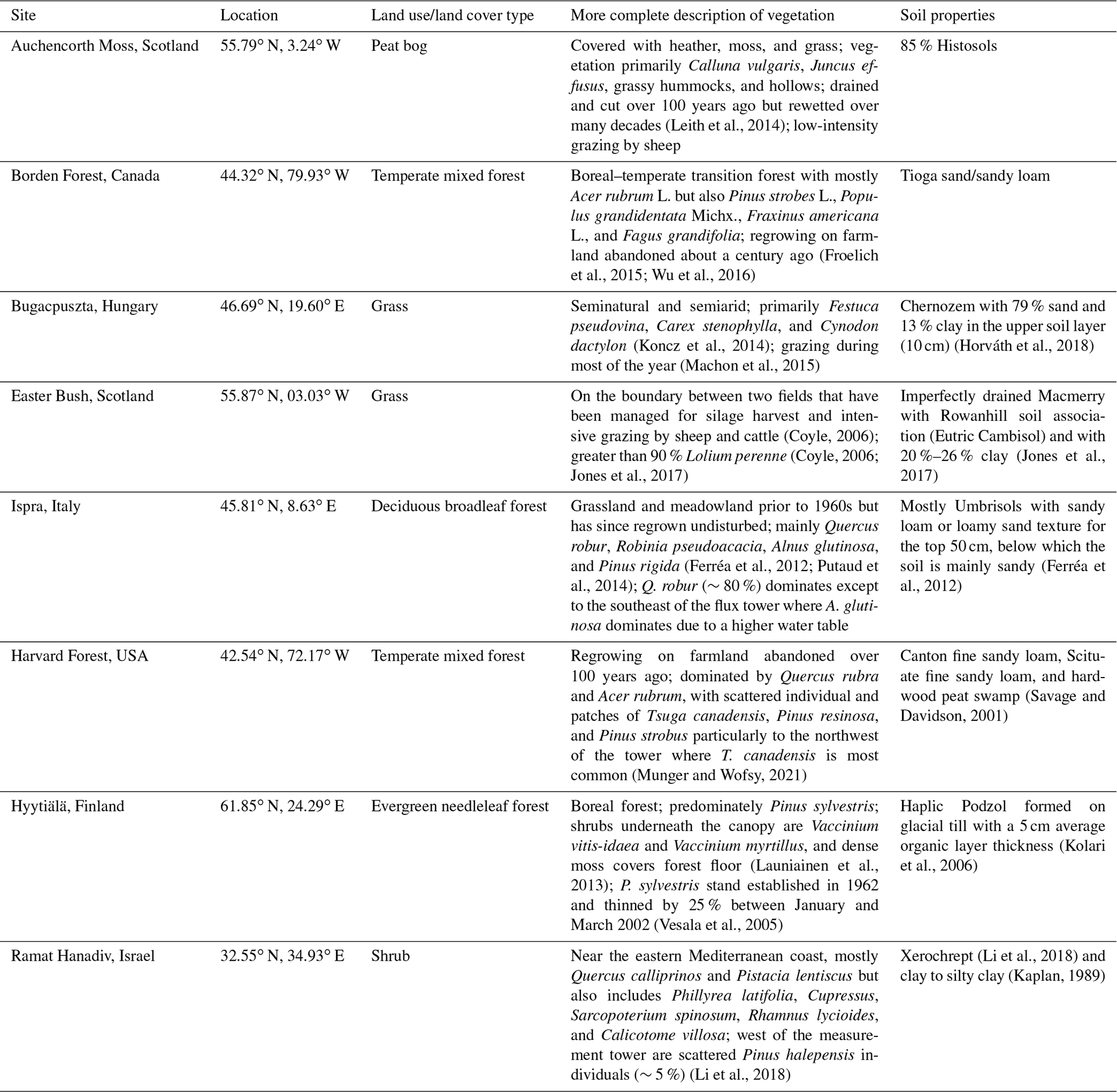
4.2 Site-specific datasets

We simulate ozone deposition velocities by driving single-point models with meteorological and environmental variables measured or inferred from measurements at eight sites. Table 2 summarizes the site locations, LULC types, vegetation composition, and soil types. The set of sites represents a variety of LULC types and climates. The sites include deciduous, evergreen, and mixed forests; shrubs; grasses; and a peat bog. Climate types include Mediterranean, temperate, boreal, and maritime and continental. Dry deposition parameterizations strongly rely on the concept that key processes and parameters are specific to LULC type. While we examine several LULC types here, we emphasize that our measurement test bed is likely insufficient to generalize the results of our study to specific LULC types; thus, we focus our discussion on individual sites. We also cannot discount the fact that differences in ozone flux methods and instrumentation and a lack of coordinated processing protocols across datasets limit meaningful synthesis of our results across sites. Table S17 summarizes details about the ozone flux measurements, the time periods examined, and the post-processing of data. Five of eight sites selected have at least 3 and up to 12 years of ozone flux data (Borden Forest, Easter Bush, Harvard Forest, Hyytiälä, and Ispra). The rest have fewer than 3 years of ozone flux data (Auchencorth Moss, Bugacpuszta, and Ramat Hanadiv) but were included to diversify the climate and LULC types examined.

Table 2Summary of ozone flux tower sites.

Download Print Version | Download XLSX

The eddy covariance technique is used for Auchencorth Moss, Bugacpuszta, Harvard Forest, Hyytiälä, Ispra, and Ramat Hanadiv. The gradient technique is used for Borden Forest and Easter Bush. The gradient technique used at Borden Forest is described in Wu et al. (2015, 2016) and was developed for Harvard Forest by comparing gradient and eddy covariance fluxes. Wu et al. (2015) shows that the gradient technique used at Borden Forest strongly overestimates ozone deposition velocities at night and during winter at Harvard Forest, as compared to the ozone deposition velocities calculated from the ozone eddy covariance flux measurements. Wu et al. (2015) also show that parameter choice can strongly influence the deposition velocities inferred from the gradient technique. Thus, seasonal and diel cycle amplitudes as well as the magnitude of observed ozone deposition velocities at Borden Forest are uncertain.

For Activity 2, we selected sites without known influences of highly reactive BVOCs on ozone fluxes. However, there may be unknown influences, especially for coniferous or mixed forests (Kurpius and Goldstein, 2003; Goldstein et al., 2004; Clifton et al., 2019; Vermeuel et al., 2021), and the magnitude of the contribution and how it changes with time are generally uncertain (Wolfe et al., 2011; Vermeuel et al., 2023). Most sites are expected to have very low NO. There may be some influences of NO on ozone fluxes at Ramat Hanadiv (Li et al., 2018) and Ispra, but the magnitude and timing of the contribution are uncertain. Constraining the contributions of highly reactive BVOCs and NO to ozone fluxes is beyond the scope of our work here.

The removal of observed hourly or half-hourly ozone deposition velocity outliers for all sites leverages a univariate adjusted box plot approach following Hubert and Vandervieren (2008), which explicitly accounts for skewness in distributions and identifies the most extreme ozone deposition velocities at each site. Non-Gaussian univariate distributions, or skewness, are present to some degree in each observational dataset used here. This method designates the most extreme 0.7 % of a normal unimodal distribution as outliers, but the exact percentage depends on the degree of skewness. For the datasets used here, which can be highly skewed, we filter 1 %–6 % of ozone deposition velocities across sites. Table S17 describes any other antecedent post-processing of the ozone deposition velocities performed for this effort.

Many dry deposition schemes include adjustments for snow. Table S18 identifies sites with snow depth (SD) measurements. Unless the single-point model directly takes SD input to infer the fractional snow coverage of the surface, we define the presence of snow as a SD greater than 1 cm. Models assume no snow if the SD is less than or equal to 1 cm or is missing.

Canopy wetness is an input to several single-point models. Others do not ingest canopy wetness explicitly as an input variable but rather indicate canopy wetness using a precipitation and/or dew indicator. For the latter type, the fraction of canopy wetness (f_wet) from datasets is not used, and models' indicators are used. Table S18 details canopy wetness measurements at each site. For sites where f_wet data are not available, f_wet values are approximated using an approach used in CMAQ (Table S18).

Soil moisture and soil properties and hydraulic variables are important for stomatal conductance as well as soil deposition processes (Fares et al., 2014; Fumagalli et al., 2016; Stella et al., 2011, 2019). Site-specific details of variables used for near-surface and root-zone volumetric soil water content are described in Table S19. A set of soil hydraulic properties (Table S20) are estimated for each site from soil texture and used across the models employing these parameters. For example, the variable B is an empirical parameter, which is calculated as the slope of the water retention curve in log space (Cosby et al., 1984), that relates volumetric soil water content to soil matric potential and can be referred to as a bulk hydraulic property of the soil (Clapp and Hornberger, 1978; Letts et al., 2000).

Overall, the core description for each site includes the key information needed to drive the single-point models: LULC type, vegetation composition, soil type, and measurement height for ozone fluxes (Table 2 and Table S17). We also describe inputs for snow, canopy wetness, h, and LAI (Table S18). Outside of the core description, other meteorological variables are measured with standard techniques, which are not discussed here. When an input variable is inferred, we detail assumptions involved in the inference because variability in inferred input variables may not be accurately represented and this may need to be accounted for when comparing simulated versus observed ozone deposition velocities.

We note that, in addition to data screening conducted by data providers, driving datasets were visually inspected and clearly erroneous values were set to missing (e.g., in one case T_a was less than −50 ^∘C). Driving datasets are not gap-filled (unless explicitly stated otherwise); therefore, simulated ozone deposition velocities have gaps whenever one or more of a model's input variables is missing. We emphasize that single-point models require different sets of input variables. Thus, output from different models may have different data gaps at a given site. Additionally, because data capture for observed deposition velocities is based on the availability of ozone flux measurements and data gaps in input variables may be different from data gaps in the ozone flux measurements, simulated deposition velocities can have different data gaps from observed deposition velocities. We address data coverage discrepancies across models and observed deposition velocities in two ways: first, we identify the time-averaged observed and simulated deposition velocities with suboptimal coverage in our results (e.g., see Fig. 1); second, we account for diel imbalances in our analysis. Both approaches are described more fully in Sect. 4.3.

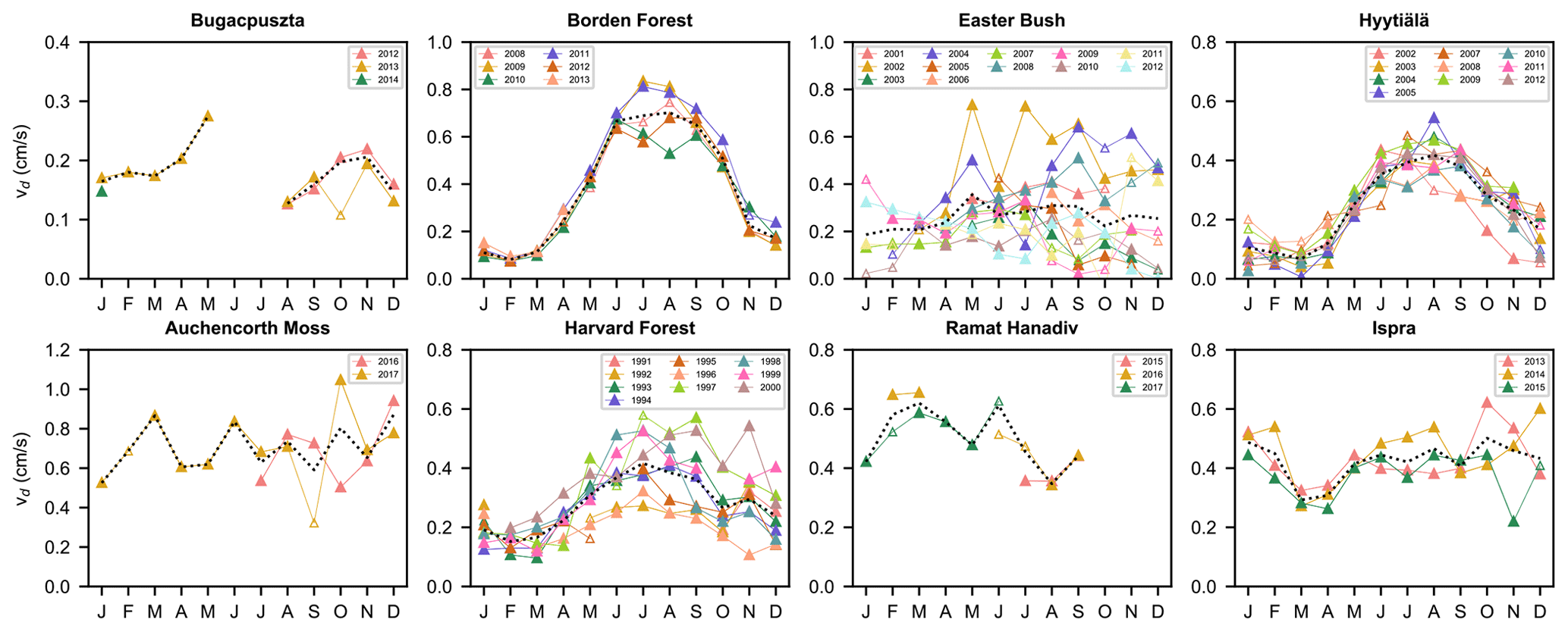
https://acp.copernicus.org/articles/23/9911/2023/acp-23-9911-2023-f01

Figure 1Monthly mean ozone deposition velocities (v_d) from the ozone flux observations. The multiyear average is in black, different years are shown using colors, and open symbols indicate months for a given year with low data capture.

Download

4.3 Creation of monthly and seasonal average observed and simulated quantities

We examine averages across 24 h, except for Ramat Hanadiv. For Ramat Hanadiv, many months have missing values during the night and morning; thus, we limit our analysis to 11:00–17:00 (all times are given in local time throughout). Across sites and analyses, we use a weighted averaging approach for daily averages that considers the number of observations for a given hour to avoid the over-representation of any given hour due to sampling imbalances across the diel cycle (e.g., more valid observations during daylight hours).

There are sometimes periods of missing ozone fluxes in the datasets. We indicate year-specific monthly averages with low data capture for observed v_d in Fig. 1. Low data capture is defined as less than or equal to 25 % data capture averaged across 24 h (or 11:00–17:00 for Ramat Hanadiv). In other words, we first compute data capture for each hour of a given month (or season) and then average across hour-specific data capture rates to compare against the 25 % threshold. We indicate multiyear monthly averages with low data capture for observations and models in Figs. 2 and 3. Note that the number of data points used in constructing monthly averages differs between models and observations, and across models. Data capture for each model depends on the availability of the specific measured input data required for driving that model. Data capture for observed v_d is based on the availability of ozone flux measurements.

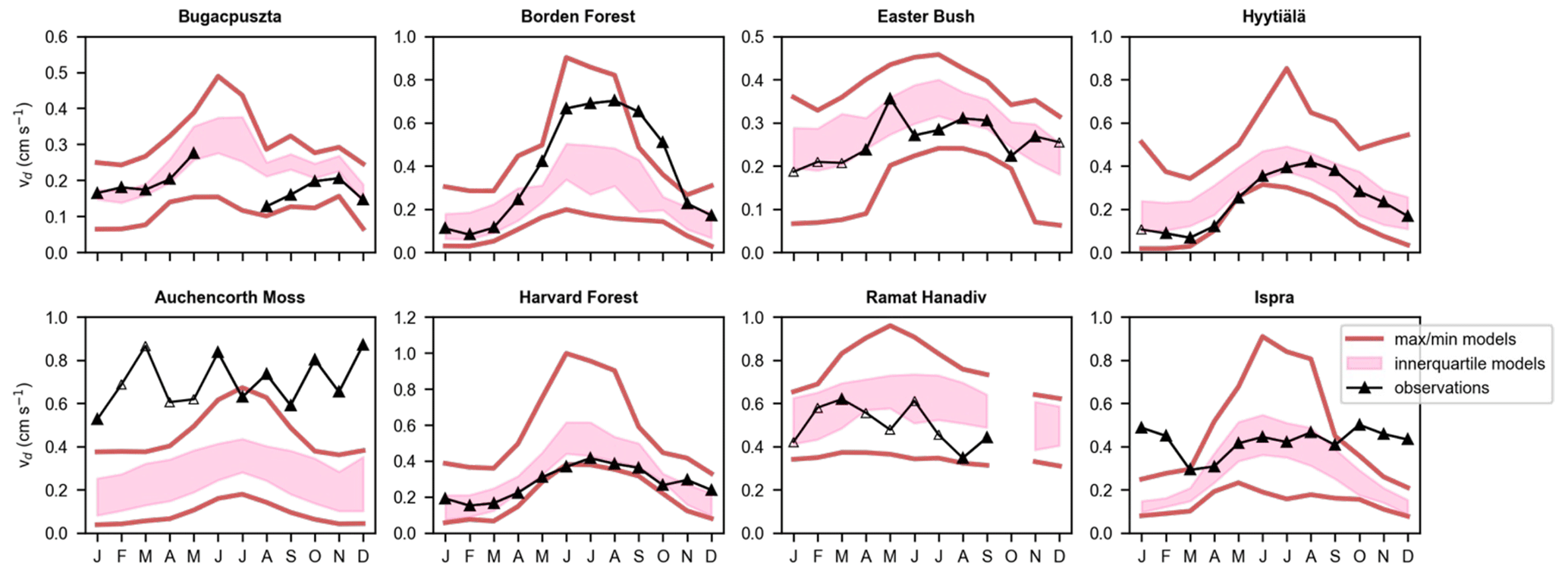
https://acp.copernicus.org/articles/23/9911/2023/acp-23-9911-2023-f02

Figure 2Multiyear monthly mean ozone deposition velocities (v_d) from ozone flux observations and single-point models. Pink shading denotes the interquartile range across models, red lines denote the minimum and maximum across monthly simulated values, and open symbols on observations indicate months with low data capture.

Download

When we examine multiyear averages, we do not consider sampling biases across years (e.g., more valid observations in 1 year over the other). Thus, more data for 1 year may skew multiyear averages towards values for that year (Fig. 1). However, results are generally similar if we include weighting by years, except when there are only a few years contributing to multiyear averages, and 1 or some of those years have low data coverage. For seasonal averages, months are not given equal weight unless stated otherwise. For example, all non-missing data for a given hour across months of the season are considered equally (e.g., the fact that there may be more data at noon in July than in August is not considered in a summertime average).

5 Results

Figure 1 shows monthly mean observed ozone deposition velocities (v_d) across years, as well as multiyear averages, at all sites. There are a variety of seasonal patterns and magnitudes of observed v_d across sites. Interannual variability is strong in terms of the standard deviation across yearly annual averages normalized by the multiyear average (range of 10 % to 60 % across sites). In some cases, periods with low data coverage contribute to apparent interannual variability and/or seasonality; thus, in these cases, the degree of interannual variability is uncertain. However, more complete ozone flux records also show strong variability from year to year and month to month, suggesting that we can expect strong interannual variability on a monthly basis to be a generally robust feature of the observations. The following discussion focuses on multiyear averages, but we briefly examine summertime (June–August) interannual variability at sites with 3 or more years of data in the individual site subsections below to establish whether models capture the range of interannual variability and/or ranking among different summers.

Figure 2 shows multiyear monthly mean v_d from observations and the spread in multiyear monthly mean v_d across models, whereas Fig. 3 shows multiyear monthly mean values from each individual model and the observations. The minimum and maximum of the monthly averages across the models bracket the observations across most sites and seasons (Fig. 2). The exceptions are Auchencorth Moss (all months except July), Borden Forest (October–November only), and Ispra (October–February only). In some cases, model outliers allow the full set of models to bracket observations (Fig. 3), which suggests limited skill of the model ensemble. If we instead consider the interquartile range across models (hereinafter, “the central models”), there are at least a few months at every site when observations fall out of range. At the same time, at every site except Auchencorth Moss, there are also at least a few months when the observations are within the range, indicating that failure of the central models to capture observations consistently across the seasonal cycle does not suggest a complete lack of skill from the model ensemble that de-emphasizes outliers. Further, the central models are very close to bracketing observations across months at Easter Bush, Hyytiälä, and Harvard Forest.

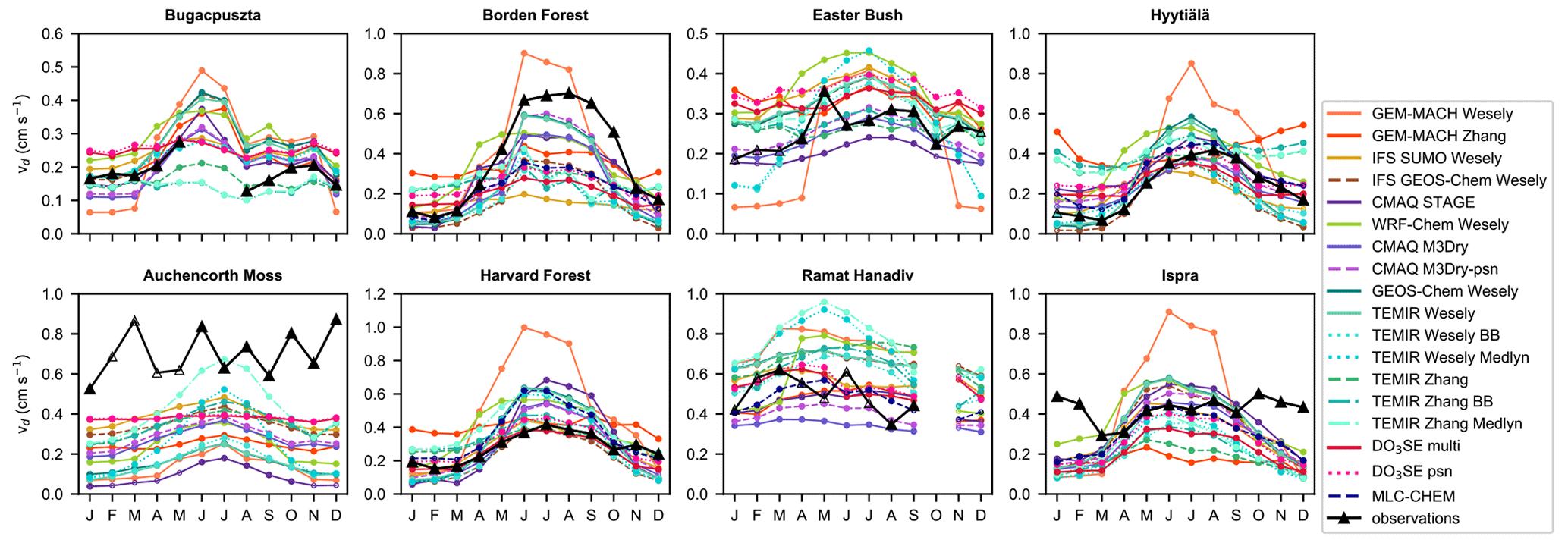
https://acp.copernicus.org/articles/23/9911/2023/acp-23-9911-2023-f03

Figure 3Multiyear monthly mean ozone deposition velocities (v_d) from ozone flux observations and single-point models. Open symbols indicate months with low data capture.

Download

The model spread in multiyear mean v_d across months and sites is large (Fig. 2). The spread in terms of the model with the highest annual average divided by the model with the lowest ranges from a factor of 1.8 to 2.3 except for Hyytiälä (2.7) and Auchencorth Moss (5). The spread in wintertime (December–February) averages is very high at some sites: Borden (10), Hyytiälä (21), Auchencorth Moss (9.1), and Harvard Forest (6.3). The spread in wintertime averages is a factor of 2 to 3.3 at other sites. The spread is typically lower during summer (June–August) than during winter, on par with annual values. We also use the 75th percentile divided by the 25th percentile as a metric of the spread. This metric for the annual average is a factor of 1.2–1.8. For winter, the metric is also lower for sites with high spreads based on all models (a factor of 3 for Borden Forest, 2.4 for Hyytiälä, 3 for Auchencorth Moss, and 2.7 for Harvard Forest), but it is still higher than the summer and annual spreads (except for Ispra).

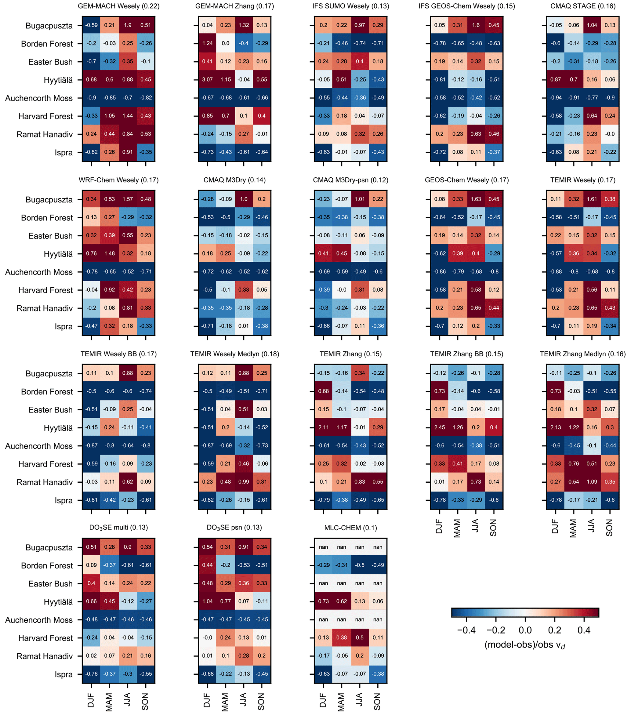
https://acp.copernicus.org/articles/23/9911/2023/acp-23-9911-2023-f04

Figure 4Seasonal mean relative biases (simulated minus observed, divided by observed) across models and sites for ozone deposition velocities (v_d), expressed as fractions. Numbers next to model names in the subpanel titles are seasonal mean absolute biases (in cm s⁻¹). DJF is December, January, and February; MAM is March, April, and May; JJA is June, July, and August; and SON is September, October, and November.

Download

Figure 4 shows the relative biases (simulated minus observed, divided by observed) across months, sites, and seasons. When we consider individual model performance, we find that no model is always within 50 % of the observed multiyear averages across sites and seasons (Fig. 4). Models are very low against observations at Auchencorth Moss, but the previous statement holds even excluding this site. In general, a key finding here is that model performance varies strongly by model, season, and site. Below, we first discuss the mean absolute biases across sites and then the drivers of seasonality across models and sites. Following this, in the subsections, we discuss each site, starting with short vegetation and then moving on to forests.

The absolute bias (simulated minus observed) averaged across multiyear seasonal averages and sites is highest for GEM-MACH Wesely (0.22 cm s⁻¹) and lowest for CMAQ M3Dry-psn (0.12 cm s⁻¹) (Fig. 4). GEM-MACH Zhang, WRF-Chem Wesely, GEOS-Chem Wesely, TEMIR Wesely, TEMIR Wesely BB, and TEMIR Wesely Medlyn are on the higher end of the spread with respect to the mean absolute bias across seasons and sites (0.17–0.18 cm s⁻¹), whereas DO₃SE multi, DO₃SE psn, IFS SUMO Wesely (0.13 cm s⁻¹), and CMAQ M3Dry (0.14 cm s⁻¹) are on the lower end, with the rest in between (0.15–0.16 cm s⁻¹). (MLC-CHEM does not simulate three sites, so we exclude it here.)

The absolute biases averaged across seasons may overemphasize model performance when v_d values are high. Given that wintertime v_d tends to be lower in magnitude than during other seasons, we also examine the wintertime mean absolute biases across sites (Fig. 4). Values are highest for GEM-MACH Zhang (0.22 cm s⁻¹), GEM-MACH Wesely (0.20 cm s⁻¹), TEMIR Wesely (0.20 cm s⁻¹), and TEMIR Wesely Medlyn (0.19 cm s⁻¹). Otherwise, model biases are below 0.16 cm s⁻¹.

Figure 5 shows the simulated multiyear wintertime and summertime mean effective conductances as well as the observed multiyear seasonal average v_d (recall that simulated effective conductances sum to simulated v_d). The three main pathways are stomata, cuticles, and soil; even when models simulate lower-canopy uptake, uptake via this pathway tends to be low. Thus, we focus on stomatal, cuticular, and soil pathways. There are three important takeaways from Fig. 5. First, models can disagree in terms of relative contributions from pathways, even when they predict similar v_d; conversely, models can agree in terms of relative contributions of pathways but predict different v_d. Second, stomatal and nonstomatal pathways both have important contributions to v_d across models and are both key drivers of variability across models. Third, models tend to disagree on cuticular versus soil contributions to nonstomatal uptake at some sites while agreeing at others.

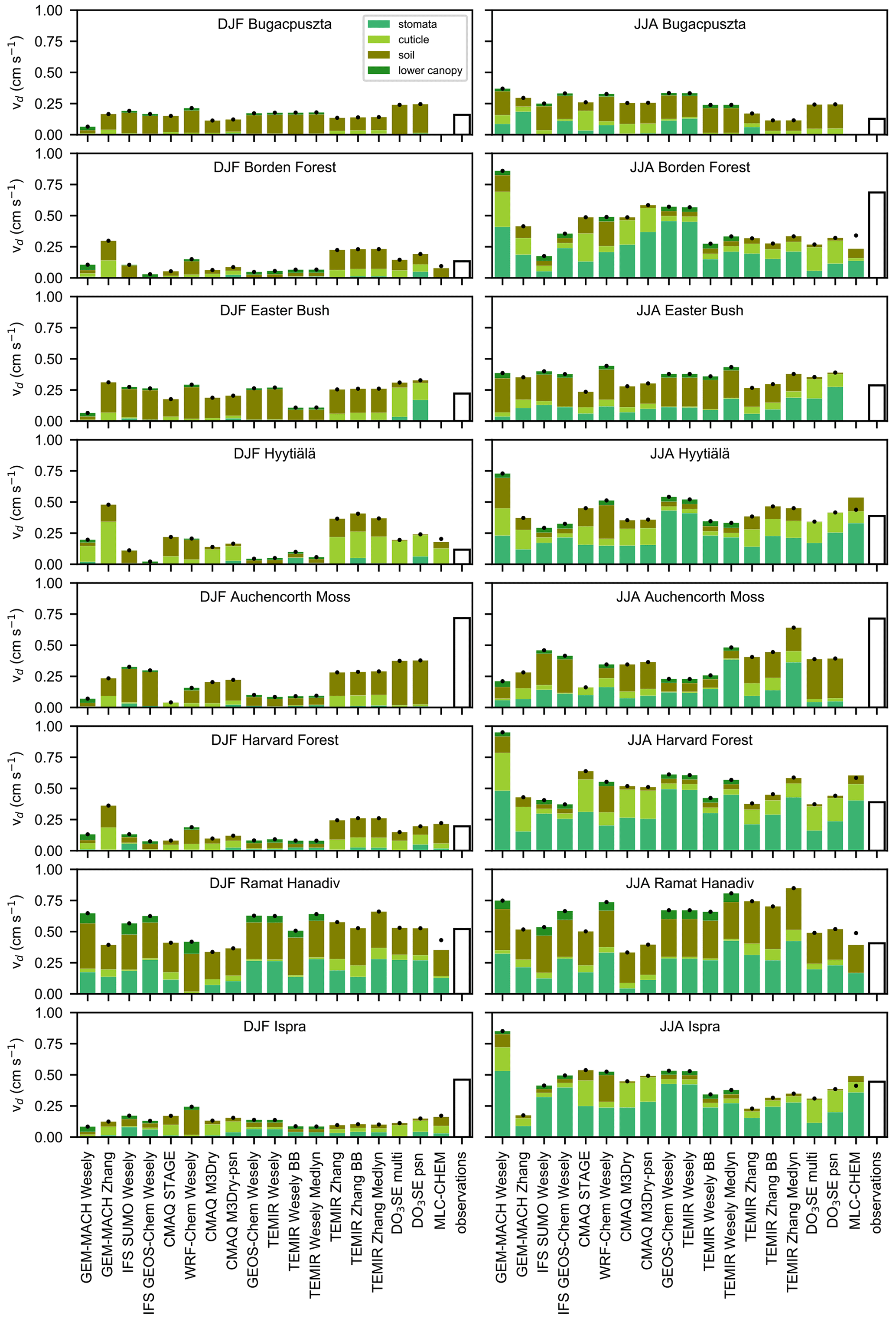
https://acp.copernicus.org/articles/23/9911/2023/acp-23-9911-2023-f05

Figure 5Multiyear seasonal mean simulated effective conductances and observed ozone deposition velocities (v_d). Black dots are simulated v_d (black dots should equal the top of the bars). DJF is December, January, and February, and JJA is June, July, and August.

Download

https://acp.copernicus.org/articles/23/9911/2023/acp-23-9911-2023-f06

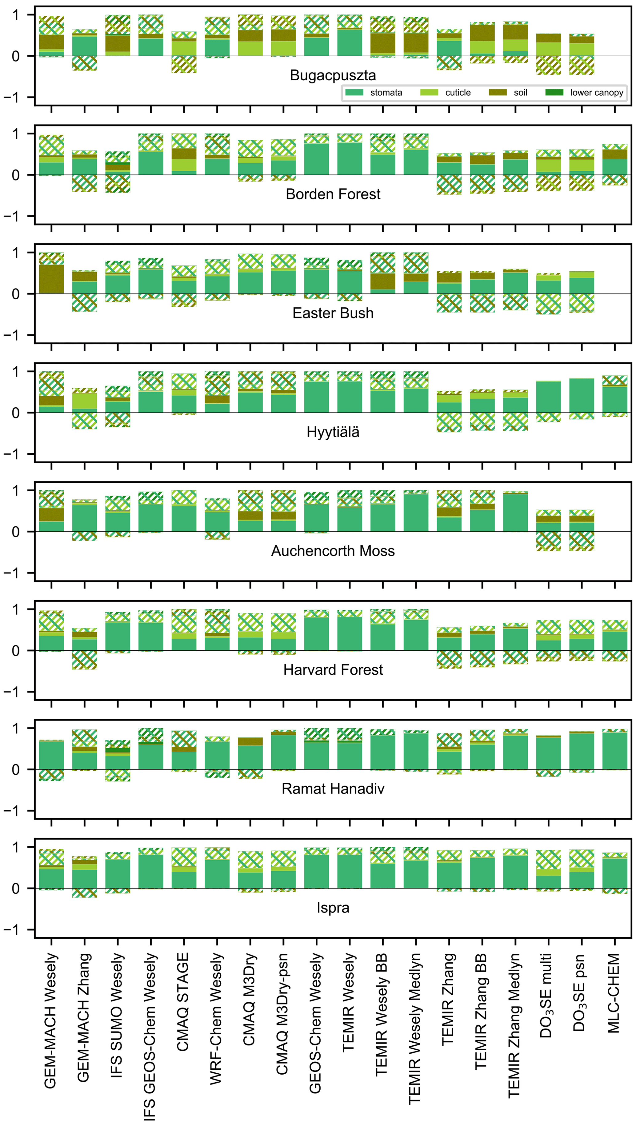
Figure 6Pathways contributing to variability across simulated multiyear monthly mean ozone deposition velocities. The variance for each effective conductance is a solid color. Twice the covariance between effective conductances is a hatched pattern (the colors of the hatching correspond to the pathways examined). Each value is normalized by the absolute value of the sum of the variances and twice the covariances so that we are comparing the pathways that drive seasonality across models in a relative sense (rather than the seasonal amplitude as well).

Download

Figure 6 shows how the multiyear mean seasonality of effective conductances contributes to the multiyear mean seasonality of simulated v_d across models. Specifically, the variance in each pathway across months is shown, as well as twice the covariance between individual pathways. Negative covariances imply offsetting seasonality between the two pathways (i.e., an anticorrelation in the seasonal cycles of two pathways that acts to dampen the total seasonality). Positive covariances mean that a positive correlation in seasonal cycles of the two pathways acts to amplify total seasonality. Values are normalized by the absolute sum of the variance and twice the covariances so that Fig. 6 does not emphasize differences in the seasonal amplitude, rather what pathways control the seasonality.

The key finding from Fig. 6 is that stomatal uptake is the most important driver of the multiyear mean v_d seasonality for most models and sites. For some models and sites, cuticular uptake also plays a role, albeit mostly just via correlations with stomatal uptake. Correlations between stomatal and cuticular pathways are mostly positive, and thus tend to amplify v_d seasonality. Exceptions are Hyytiälä and Easter Bush, where some models show anticorrelations between stomatal and cuticular uptake seasonal cycles. With a few exceptions (e.g., at Easter Bush and for the GEM-MACH Wesely and DO₃SE models), soil uptake tends to play a more minor role.

In general, the parameters and dependencies driving simulated v_d seasonality are model-dependent. Expected dominant influences include changes in initial resistances with season, cuticular and stomatal dependencies on LAI, stomatal dependencies on soil moisture, temperature response functions (used in Wesely, 1989, to decrease nonstomatal deposition pathways at cold temperatures), and changes with snow.

Figure 7 shows how multiyear monthly mean v_d changes with LAI, for both the models and the observations. Multiyear monthly mean observed and simulated v_d generally increases with LAI across sites during at least some time periods of plant growth (Fig. 7). In general, however, the relationship between v_d and LAI on monthly timescales is nonlinear for both observations and models, distinct between observations versus models, and distinct across models. Many models show a strong sensitivity to the LAI, which has been pointed out in previous work (Cooter and Schwede, 2000; Charusombat et al., 2010; Schwede et al., 2011; Silva and Heald, 2018). Our analysis here, combined with past work, suggests that advancing predictive ability requires a better understanding of observed v_d–LAI relationships in terms of seasonality and site-to-site differences.

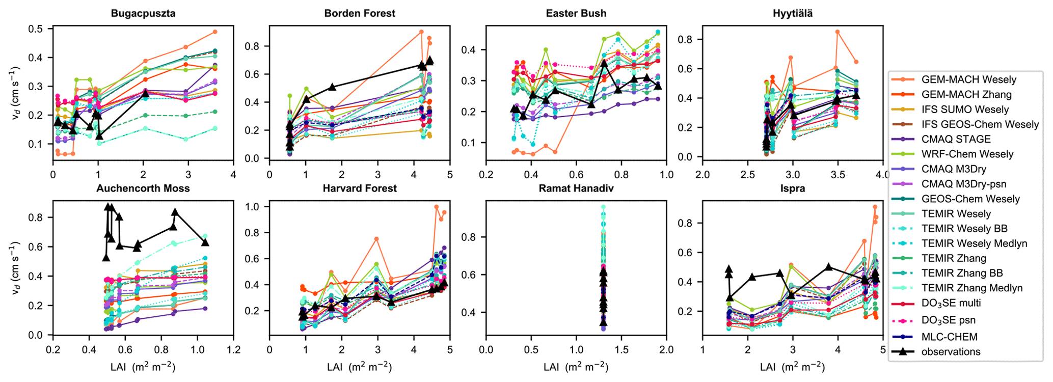
https://acp.copernicus.org/articles/23/9911/2023/acp-23-9911-2023-f07

Figure 7Multiyear monthly mean ozone deposition velocities (v_d) versus the leaf area index (LAI).

Download

https://acp.copernicus.org/articles/23/9911/2023/acp-23-9911-2023-f08

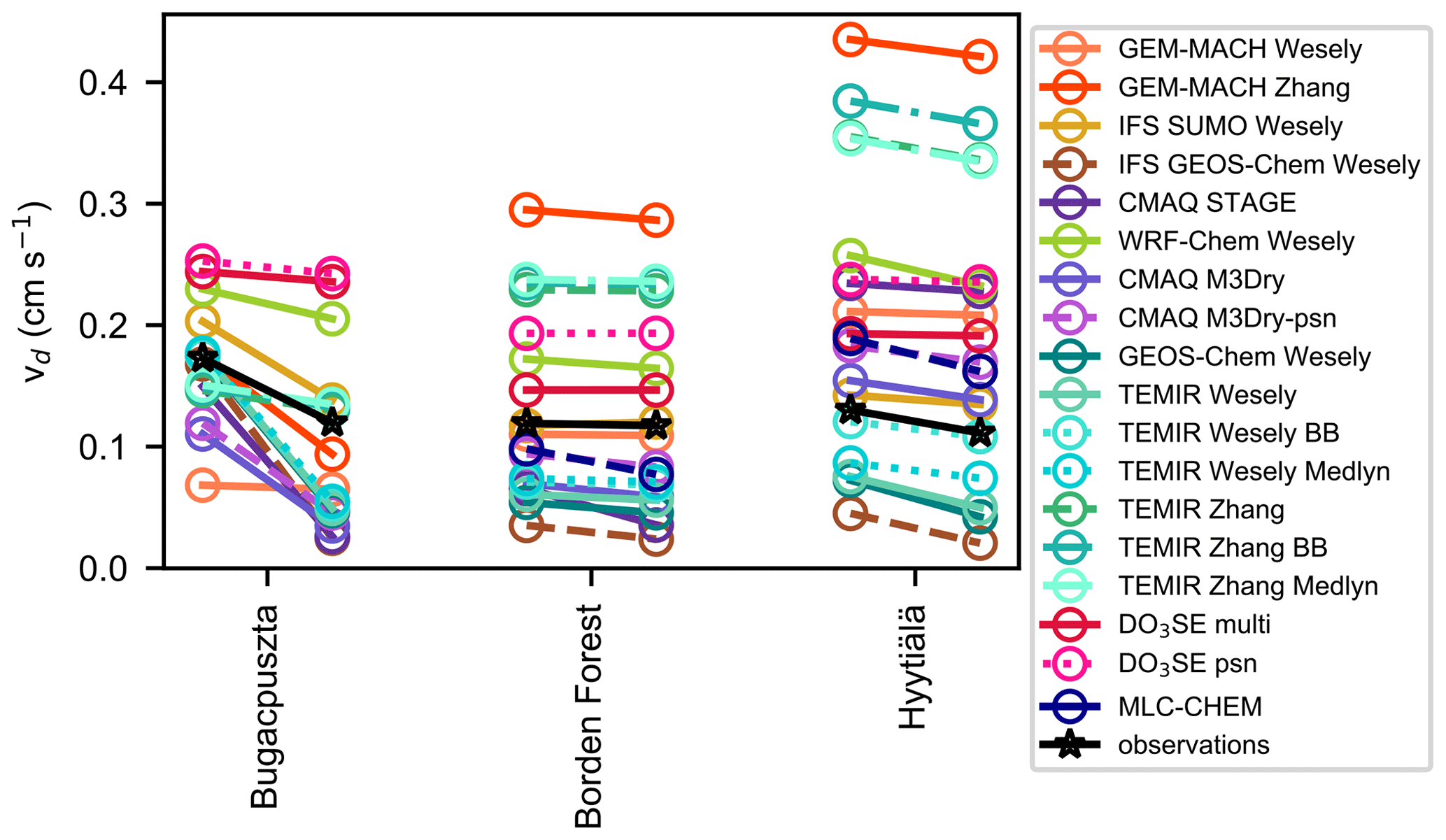
Figure 8Multiyear mean ozone deposition velocity (v_d) during all conditions versus when the snow depth is greater than or equal to 1 cm for sites with snow depth records and sufficient time with snow (25 %, averaged across hours per month). Months considered are December–February for Bugacpuszta, December–February for Borden Forest, and November–March for Hyytiälä. Months are given equal weight in the averages.

Download

Figure 8 shows snow's impact on the multiyear mean v_d at sites with snow depth records and sufficient snowy periods. Observations suggest modest reductions with snow at Bugacpuszta and Hyytiälä but not much change at Borden Forest. At Borden Forest, some models show decreases, whereas others show little change. At Hyytiälä and Bugacpuszta, some models capture decreases with snow despite biases, whereas other models understate or exaggerate decreases. Observed reductions with snow are larger at Bugacpuszta than Hyytiälä, and many models capture this. Findings with respect to Borden Forest may reflect that snow is not measured there, rather 15 km away, and thus these measurements do not reflect the exact local conditions. Even though some models do not capture the magnitude of the observed v_d decreases with snow, Fig. 8 shows that models' inability to capture the magnitude of wintertime values (snow or snow-free) at a given site is a much larger problem than models' inability to capture responses to snow, at least at these three sites. The relative model spread (based on the standard deviation across models divided by the average) does not change substantially under snowy versus all conditions, except at Bugacpuszta (27 % versus 70 %), further underscoring the need to better understand wintertime v_d in a more general sense.

The relatively low magnitude of snow-induced observed v_d changes indicates that snow-induced changes are not the main driver of observed v_d seasonality (Fig. 8). For example, observed changes with snow are a small fraction of the observed absolute seasonal amplitude of multiyear monthly averages at these sites, at least for Hyytiälä and Borden Forest. We also note that models simulate v_d reductions with snow at Hyytiälä and Bugacpuszta even when snow is not model input, suggesting that other model dependencies (e.g., temperature response functions) may lead to changes coincident with snow. Recent papers have suggested that better snow cover representation may be key with respect to capturing v_d spatial variability at regional scales and regional average seasonal cycles as well as changes with climate change (Helmig et al., 2007; Andersson and Engardt, 2010; Matichuk et al., 2017; Clifton et al., 2020b). Despite insufficient data to examine spatial variability or responses to climate change, our analysis suggests that it is important to understand drivers of wintertime v_d other than snow.

5.1 Bugacpuszta

Bugacpuszta is a semiarid and seminatural grassland in Hungary that experiences grazing during most of the year. In terms of variability across models, the model spread based on the model with the highest annual average v_d divided by the model with the lowest is a factor of 2.1 (2.8 during summer and 2.2 during winter); however, based on the interquartile range, this value is a factor of 1.3 (1.2 during summer and 1.3 during winter). This model spread at Bugacpuszta is on the lower end of the estimates across the sites examined.

A longer ozone flux data record is needed to assess the interannual variability at Bugacpuszta. Bugacpuszta has only 1 year of data during February–May (from 2013), 2 years of data during August–December (from 2012 and 2013), and 2 years of data during January (from 2013 and 2014) (Fig. 1). Data are always missing during June and July. For time periods with 2 years of data, observed monthly mean v_d values are very close in magnitude between years. The exception is October, for which 2013 values are half of the 2012 values. However, October 2013 has very low data coverage (only ∼2–3 d of coverage), and hourly values exhibit high uncertainty compared with other months (not shown). Agreement between both years for months with sufficient data coverage may suggest that there is low interannual variability at this site; however, more data are really needed to make this assessment, as well as in-depth analyses of shorter-term variability (e.g., diel cycles). In the following, we focus on the “multiyear averages” at this site, acknowledging that there are only 2 years of data during 6 months of the year (and 10 months total with data).

Without June and July observations, we cannot fully assess seasonality at Bugacpuszta. Therefore, we evaluate seasonality across other months. The observed seasonal cycle for the months with data is as follows: v_d maximizes during May, following an increase from March, and minimizes during August, after which v_d increases to November and levels off from December to February (Fig. 1). Seasonal patterns are similar across many models, with midsummer peaks after slow increases from winter and similar values from August to November (Fig. 3). Despite similar seasonal patterns across the models as well as fair agreement in the relative seasonal amplitude across the models (Fig. 9), the models disagree with respect to the pathways dominating the seasonal cycle (Fig. 6). Notably, models disagree the most in terms of the pathway(s) driving seasonality at Bugacpuszta relative to other sites, suggesting that changes in individual pathways on seasonal timescales at this location may be a key uncertainty.

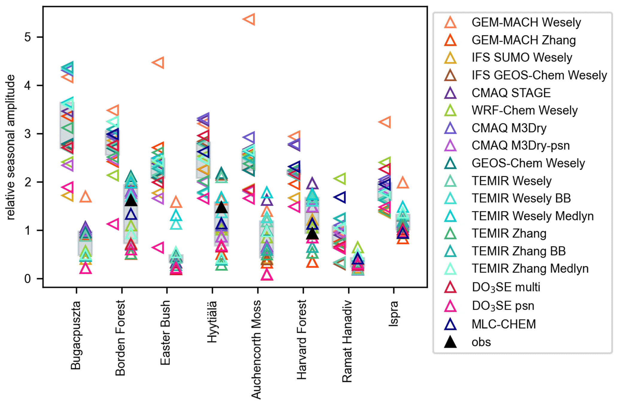
https://acp.copernicus.org/articles/23/9911/2023/acp-23-9911-2023-f09

Figure 9Relative seasonal amplitudes of multiyear monthly mean stomatal uptake (sideways triangles) and ozone deposition velocities (upwards triangles) across models, defined as the maximum across months of multiyear monthly averages minus the minimum, divided by the average. Black triangles denote the relative seasonal amplitude of observations for sites with wintertime minima and summertime maxima. Gray shading denotes the interquartile range across models.

Download

The central models bracket observed v_d at Bugacpuszta during December–May but are too high against the observations during August and September (and only slightly too high during October and November) (Fig. 2). Two clear model outliers during the warm months are the TEMIR Zhang models (Fig. 3), which show relatively low soil and cuticular uptake (Fig. 5). TEMIR psn also shows no stomatal uptake, following very low input root-zone soil moisture (below prescribed wilting point). While the TEMIR Zhang models are clear model outliers during the warm months, they allow the complete set of models to bracket observations during August–November, because the other models are mostly too high (or, in a few cases, just right). Without June and July ozone fluxes, however, it is unclear how the TEMIR Zhang models alter the summertime performance of the model spread.

Only eight models show substantial summertime stomatal uptake at Bugacpuszta (Fig. 5). There is no summertime stomatal uptake simulated by the TEMIR psn, IFS SUMO Wesely, or DO₃SE models, and very little summertime stomatal uptake is simulated by CMAQ STAGE, CMAQ M3Dry, and CMAQ M3Dry-psn. Only these models employ soil moisture dependencies on stomatal conductance (MLC-CHEM does as well but does not simulate values at Bugacpuszta); these models simulate little to no stomatal uptake at Bugacpuszta because input soil moisture is below the prescribed wilting point. We emphasize that the wilting point, which is not a directly measurable quantity, is uncertain across sites. Nonetheless, the magnitude of stomatal uptake at this site is a clear uncertainty. If we instead focus on the models with substantial summertime stomatal uptake, we can see that they show a large spread in the stomatal fraction of v_d – from 12.5 % to 40 % with one model simulating 60 % (Fig. 12) – and produce distinct stomatal uptake seasonal cycles (Fig. 10). On the other hand, many models show similar v_d seasonal cycle shapes (Fig. 3) but dissimilar stomatal uptake seasonal cycle shapes. These results suggest that nonstomatal uptake seasonality plays a role in normalizing differences in v_d seasonal cycles across models, and the models are more distinct than implied by v_d alone.

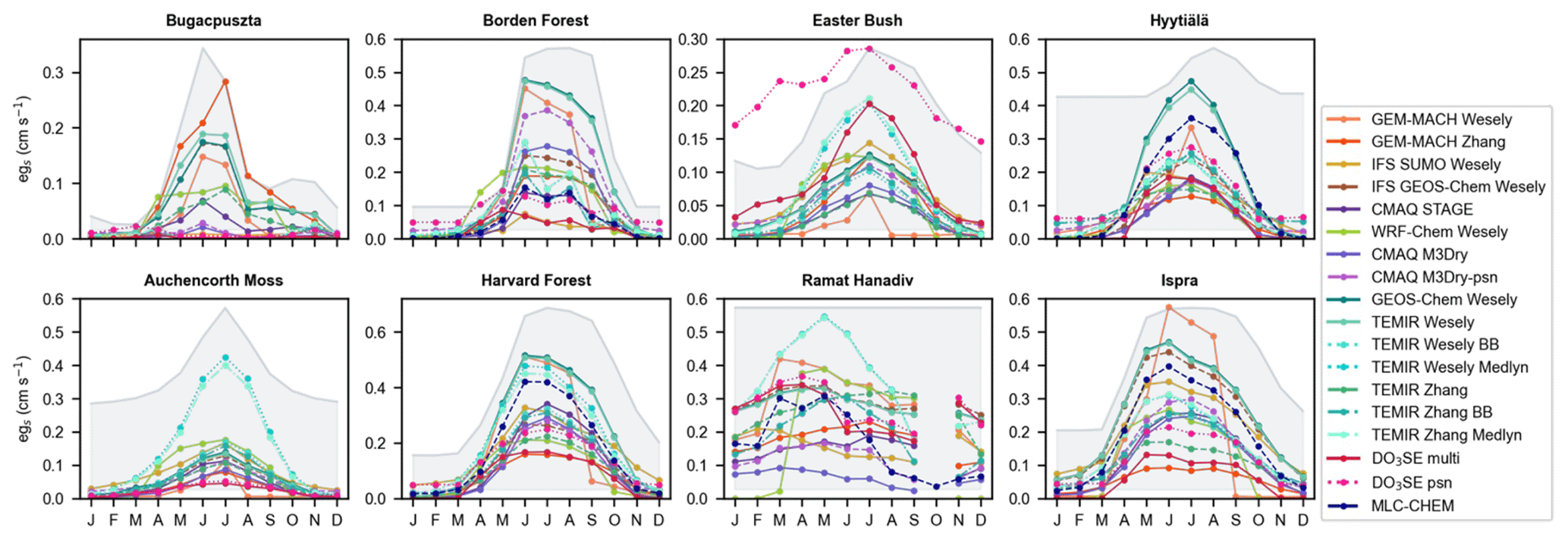
https://acp.copernicus.org/articles/23/9911/2023/acp-23-9911-2023-f10

Figure 10Multiyear monthly mean effective stomatal conductance (eg_s) from single-point models. Gray shading denotes the multiyear monthly mean LAI (used to emphasize seasonality in this variable; y ranges are not given).

Download

https://acp.copernicus.org/articles/23/9911/2023/acp-23-9911-2023-f11

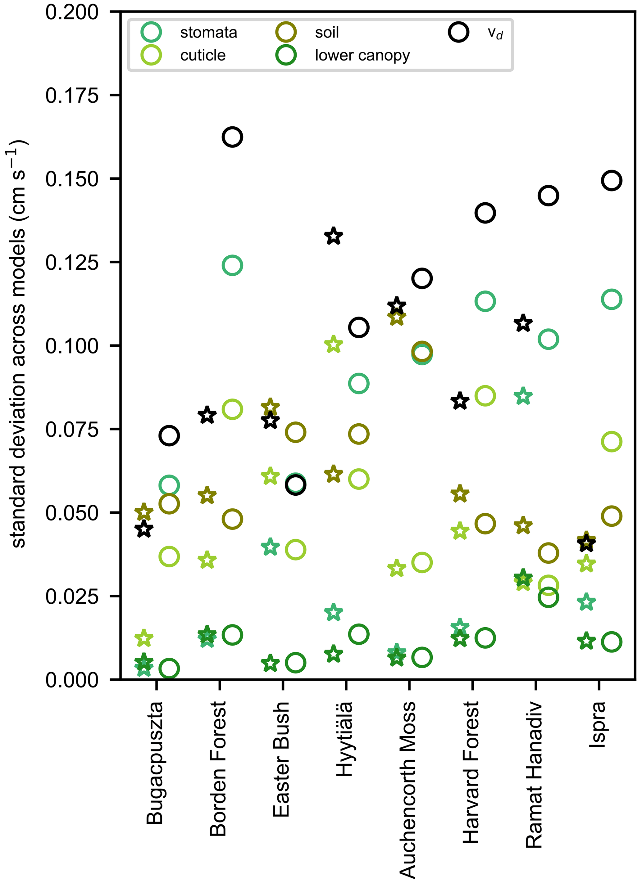
Figure 11Model spread (standard deviation) across multiyear seasonal mean ozone deposition velocities (v_d) and effective conductances for DJF (stars) and JJA (circles). DJF is December, January, and February, and JJA is June, July, and August.

Download

Bugacpuszta has the most similar summertime model spreads across the top three deposition pathways relative to other sites (except Hyytiälä) (Fig. 11), suggesting a high degree of uncertainty in the magnitude of all pathways during the warm months. Most models show substantial summertime contributions from soil uptake, but the magnitude of soil uptake varies across models (Fig. 5). In contrast, for the summertime cuticular and stomatal pathways, models disagree as to whether contributions are substantial as well as disagreeing on the magnitude of uptake. For example, like how some models show very low stomatal uptake (as discussed above), some models show negligible cuticular uptake. Establishing whether there should be summertime stomatal and/or cuticular uptake at Bugacpuszta would be a first step towards further constraining models.

The multiyear monthly mean LAI at Bugacpuszta shows a sharp summer peak, maximizing during June (∼3.6 m² m⁻²) (Fig. 10). Values are similar during August to November and then decrease from November to March, with a minimum during March. Observed v_d is missing for LAI values greater than 2 m² m⁻² (corresponding to June and July). There is no discernable observed v_d–LAI relationship for LAI values below 1 m² m⁻², and models capture this (Fig. 7). Observations show a strong v_d increase from 1 to 2 m² m⁻². Models show an increase, but most do not capture the large observed slope. This is especially true for models with soil moisture dependencies on stomatal conductance, implying that, during at least some periods of high vegetation density, there should not be soil moisture stress or not as strong soil moisture stress as simulated by some models.

Models simulate that soil uptake dominates wintertime v_d at Bugacpuszta (Fig. 5). The exception is GEM-MACH Wesely, which underestimates wintertime v_d. Wintertime stomatal fractions of v_d can be up to 10 % (due to low v_d overall) but are mostly within 0 %–5 %. Because the central models capture wintertime v_d (Fig. 2) and models also agree that soil uptake dominates, some models may have some skill during cooler months. However, there is variability in soil uptake across models (Fig. 11). Models largely capture observed wintertime v_d decreases with snow, with most slightly overestimating the change but a few (the DO₃SE models, WRF-Chem Wesely, TEMIR Zhang, and GEM-MACH Wesely) underestimating it (Fig. 8). Future attention to the noncentral models should focus on better capturing wintertime nonstomatal uptake generally at this site, rather than changes with snow.

A key outstanding question at Bugacpuszta is as follows: should models simulate low stomatal uptake throughout summer or only during late summer? Most model values are too high compared with observations during August and September. This includes models employing soil moisture dependencies on stomatal conductance (and, thus, simulating very low to no stomatal uptake), implying an overly high simulated nonstomatal uptake. Continuous year-round ozone flux observations, especially during periods of the growing season with and without moisture stress, are needed to better assess model performance at Bugacpuszta. Independent measures of stomatal conductance during periods of missing ozone fluxes would be useful in constraining the absolute stomatal portion of dry deposition, but further constraining nonstomatal uptake, which models indicate is an important fraction of summertime v_d (despite disagreeing on the exact pathway), requires additional ozone flux measurements.

5.2 Auchencorth Moss

Auchencorth Moss is a peat bog in Scotland that is covered with heather, moss, and grass. The model spread in terms of the model with the highest annual average v_d divided by the model with the lowest is a factor of 5 (4.3 during summer and 9.1 during winter); however, based on the interquartile range, this value is a factor of 1.6 (1.5 during summer and 3 during winter). Across sites, for the annual metrics, Auchencorth Moss has the largest spread for the maximum/minimum metric and the second largest for the interquartile range.

There is no clear shape of the observed v_d seasonal cycle at Auchencorth Moss (Fig. 1). Whether this is true on a climatological basis is unclear due to (1) data incompleteness during the 2-year period – observed values during February–May have low data capture mostly because data are missing during 2016 – and (2) strong interannual variability when there are data and (3) the fact that there are only 2 years of data. A longer and more complete ozone flux record is needed to fully assess interannual variability as well as seasonality at Auchencorth Moss. Below, we focus on multiyear averages, acknowledging that only half the months of the year have 2 years of data.

A key finding is that models do not capture the high values of v_d that are observed year-round at Auchencorth Moss (Fig. 2). The exception is TEMIR Zhang Medlyn during July. Auchencorth Moss is the only site examined with negative biases (> 30 % of observed multiyear seasonal averages) across seasons and models (except for TEMIR Zhang Medlyn during July) (Fig. 4). Biases tend to be smallest during summer and largest during winter because many models simulate peak v_d during warm months (Fig. 3). Notably, models differ substantially with respect to their relative seasonal amplitudes, with a very even and wide distribution in relative seasonal amplitude across models (Fig. 9), especially relative to other short-vegetation sites.

Simulated v_d seasonality is mostly due to stomatal uptake (Fig. 6). Some models show that soil uptake plays a role, and all but two models show moderate contributions from correlations between pathways. The seasonality shape of stomatal uptake is very similar across most models, as is the magnitude of stomatal uptake throughout the year (Fig. 10). Major exceptions are the TEMIR Medlyn models, which show peak values of around 0.4 cm s⁻¹ in contrast to the rest that average just under 0.1 cm s⁻¹. For the relative seasonal amplitudes in stomatal uptake, the spread across the central models is low (Fig. 9). The value for GEM-MACH Wesely is very high (> 5), with other models' values spanning a factor of 1.75 to 3. Models deviating from the rest with respect to stomatal uptake's seasonality shape are GEM-MACH Zhang (a strong peak during July and near-zero during August and after) and DO₃SE (low during summer) as well as WRF-Chem Wesely and IFS SUMO Wesely (the latter two are similar and higher than others, especially during spring).

While high summertime stomatal uptake combined with moderately high year-round nonstomatal uptake distinguishes TEMIR Zhang Medlyn from the other models (Fig. 5), we see the best agreement between this model and observations during the warm months. However, TEMIR Zhang Medlyn does not capture observed seasonality (or lack thereof). Thus, TEMIR Zhang Medlyn may have more skill during summer than other models; however, like other models, TEMIR Zhang Medlyn struggles with seasonality. Future work should establish whether there is strong seasonality in stomatal uptake coupled with offsetting seasonality in nonstomatal uptake at Auchencorth Moss or whether stomatal uptake should be higher year-round.

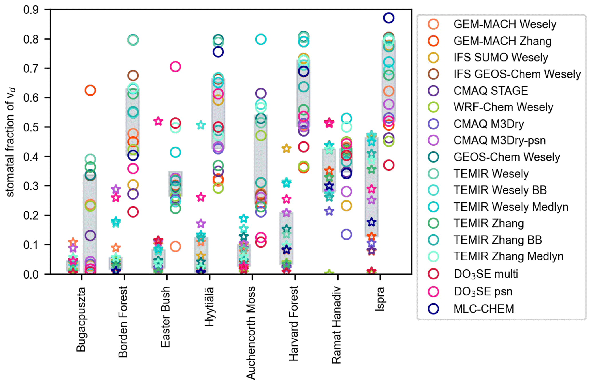
https://acp.copernicus.org/articles/23/9911/2023/acp-23-9911-2023-f12

Figure 12Multiyear seasonal mean stomatal fraction of ozone deposition velocities (v_d) across models during DJF (stars) and JJA (circles). Gray shading denotes the interquartile range across models. DJF is December, January, and February, and JJA is June, July, and August.

Download

For soil uptake, the model spread is large and similar between summer and winter (Fig. 11). During summer, the spread in stomatal uptake is on par with soil uptake; spreads for stomatal and soil uptake are the highest across pathways. During winter, the spread in stomatal uptake is very low, and the spread in soil uptake is the highest. Wintertime stomatal fractions vary from 0 % to 20 % across models (Fig. 12). Models except CMAQ STAGE simulate non-negligible soil uptake (Fig. 5). However, during summer, models disagree on the soil contribution to v_d (0 %–80 %) as well as the magnitude of soil uptake. In contrast, during winter, models agree that soil uptake contributes substantially to v_d (> 60 %) (apart from CMAQ STAGE and GEM-MACH Wesely) but disagree on the magnitude of soil uptake. Snow depth is measured at Auchencorth Moss, but data are missing during half of the ozone flux period, and there is not a substantial amount of time with snow when there are measurements.

Models estimate very low to moderate cuticular uptake at Auchencorth Moss (Fig. 5), which is consistent across low-vegetation sites. Moderate values of cuticular uptake are simulated by the GEM-MACH Zhang and TEMIR Zhang models, and values are similar between summer and winter. Otherwise, models simulate very little cuticular uptake during winter and low cuticular uptake during summer. Nonetheless, the model spread in cuticular uptake is similar between seasons. Summertime stomatal fractions vary across the central models from 25 % to 55 % (Fig. 12). Aside from one model simulating 80 % and two models around 10 %, half are around 20 %–30 % and the other half are around 45 %–60 %. There is a clear division across models in that no model simulates stomatal fractions between 32.5 % and 45 %. The dichotomy seems to be due to variability in both stomatal and soil uptake across models, consistent with high summertime model spreads for these pathways (Fig. 11).

Despite an unclear observed v_d seasonal pattern at Auchencorth Moss, the relationship between the monthly mean LAI and v_d may provide insights into model performance. With strong observed v_d variations at low LAI values (less than 0.6 m² m⁻²), there is no relationship, but there is a positive relationship at moderate LAI values (in the range of 0.6 to 0.9 m² m⁻²) (Fig. 7). Observations then show that v_d decreases with LAI increases above 0.8 m² m⁻², but there is only one data point here. Most models seem to capture the observed relationship at moderate LAI values as well as that there should not be a relationship at low LAI values. However, some models (e.g., the TEMIR models) overestimate the increase's slope at moderate LAI values. Thus, some models may have some skill with respect to simulating seasonality in cuticular and/or stomatal uptake. Nonetheless, strong observed v_d variability at low LAI values and changes with LAI during peak vegetation density require a better understanding. With observational constraints on stomatal uptake, we will be able to understand whether nonstomatal uptake should be higher year-round and/or seasonality in nonstomatal uptake should act to offset seasonality in stomatal uptake.

We close by emphasizing that very high observed v_d values at Auchencorth Moss are uncertain – there is strong interannual and day-to-day variability but a lot of missing data. The peat/bog LULC type does not have many ozone flux measurements at other sites that could be used to provide additional context to Auchencorth Moss measurements. Schaller et al. (2022) show that v_d ranges from 0.05 cm s⁻¹ at night to 0.45 cm s⁻¹ during the day in July 2017 at a peatland in northwestern Germany. El Madany et al. (2017) look at ozone fluxes at the same site during 2014 but do not present v_d values. Fowler et al. (2001) present older measurements at Auchencorth Moss, estimated with the gradient technique (eddy covariance is used for the data examined here), showing much lower observed v_d than examined here (e.g., winter and fall values here are twice what they are during 1995–1998, summer values are almost twice as high, and spring values are higher but not twice as high). It is not clear what drives the higher, more recent v_d measurements at Auchencorth Moss analyzed in this study, and more detailed analysis is needed to figure it out. In general, building an understanding of ozone dry deposition for this LULC type provides a key test of the understanding of soil uptake and of its dependence on its expected drivers (soil organic carbon and water content), given that peat/bog soils are organic-rich and wet.

5.3 Easter Bush

Easter Bush is a managed grassland in Scotland that is used for silage harvest and intensive grazing. In terms of variability across models, the spread based on the model with the highest annual average v_d divided by the model with the lowest is a factor of 1.8 (1.8 during summer and 3.0 during winter); however, based on the interquartile range, this value is a factor of 1.3 (1.3 during summer and 1.4 during winter). Model spreads at Easter Bush are some of the lowest compared with other sites.

Easter Bush has one of the longest ozone flux records (Clifton et al., 2020a), and it has the longest record examined here as well as the strongest interannual variability. For example, the coefficient of variation across years is on average 60 % across months. In contrast, other sites show coefficients of variations across years from 10 % to 30 %. There is also strong interannual variability in the observed seasonal cycle's shape at Easter Bush (Fig. 1). As for other sites with long-term records, we focus on multiyear averages but also touch on summertime interannual variability. Some models capture some low summers, but models do not capture high summers (except GEOS-Chem Wesely, IFS GEOS-Chem Wesely, and TEMIR Wesely, which capture 1 high year) and underestimate interannual spread (Fig. 13). Future work should focus on understanding observed interannual variability and should consider that interannual variability changes strongly by month, both in terms of the spread across years and the ranking of years.

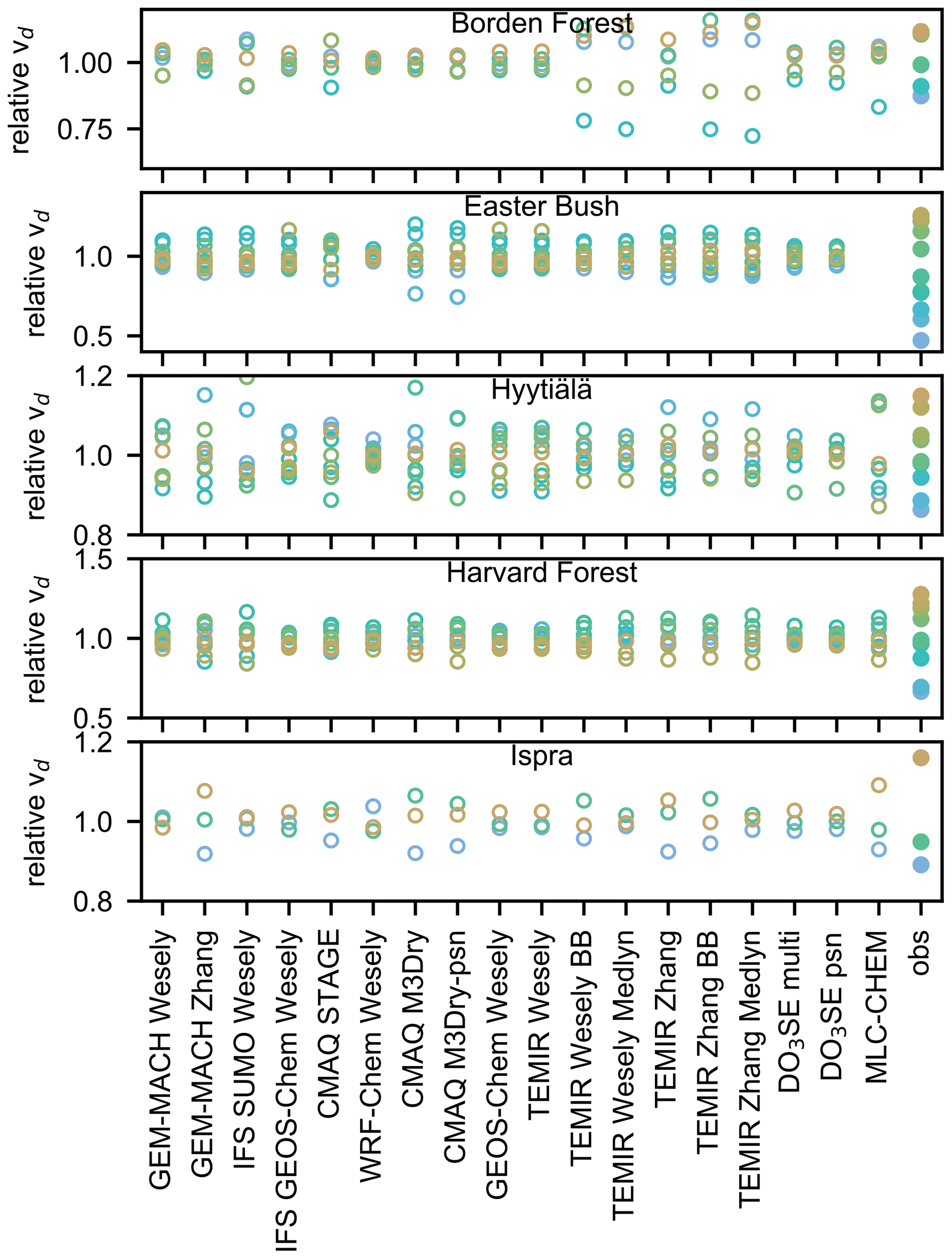
https://acp.copernicus.org/articles/23/9911/2023/acp-23-9911-2023-f13

Figure 13Simulated and observed yearly summertime mean ozone deposition velocities (v_d) for sites with records of at least three summers. Values are normalized by the multiyear average of the respective model or observations to emphasize ranking and spread across years. Colors rank yearly values from low (blue) to high (gold) for the observations. The model year is not shown when the observed year is missing. The highest year for Easter Bush is not shown because it is very high (2 times the multiyear mean observed value).

Download

The central models' spread largely brackets the observed multiyear monthly values across months. Specifically, observed values sit mostly on the lower end of or just below the central models' spread, except during May, November, and December when observed values are on the higher end (Fig. 2). Only CMAQ STAGE consistently shows lower v_d than observed, but the relative bias is low (−18 % to −30 %) (Fig. 4). During winter, GEM-MACH Wesely and TEMIR Wesely psn are too low, and the relative biases are substantial (−51 % to −70 %). With a few exceptions (i.e., winter for GEM-MACH Wesely and TEMIR Wesely psn and summer for WRF-Chem Wesely and TEMIR Wesely Medlyn), models are within ±50 % of observed seasonal averages.

Overall, the following suggests that models may have skill with respect to simulating climatological v_d seasonality at Easter Bush, aside from a clear set of outliers. There is a weak warm-season peak in observed v_d (Fig. 1). Models show weak warm-season maxima (Fig. 3) and relatively similar relative seasonal amplitudes (Fig. 9). However, some models are clear outliers. For example, GEM-MACH Wesely and TEMIR Wesely psn show particularly strong relative seasonal amplitudes (Fig. 9), in part due to low wintertime v_d. The absolute standard deviation across models for v_d is higher during winter than during summer (Fig. 11). This only happens at Easter Bush and Hyytiälä; however, as noted above, the wintertime model spread reduces when considering the full versus interquartile range, suggesting that low outliers may drive the large standard deviation across models.

For most models, the primary driver of v_d seasonality is stomatal uptake (Fig. 6). However, individual contributions from stomatal uptake barely contribute for GEM-MACH Wesely and TEMIR Wesely BB. Several models, including GEM-MACH Wesely, GEM-MACH Zhang, the TEMIR Wesely models, and TEMIR Zhang models, simulate large contributions from soil uptake individually and/or via correlations with other pathways. Only two models, in contrast to seven at the other grassland examined (Bugacpuszta), suggest that individual contributions from cuticular uptake matter for seasonality.

Most models are similar in terms of magnitude and seasonality shape of stomatal uptake (Fig. 10), as well as relative seasonal amplitudes (Fig. 9). Exceptions are GEM-MACH Wesely (a very strong peak during July and almost zero after July, thereby showing an anomalous seasonal amplitude), TEMIR Medlyn (much higher than other models during the warm months), and IFS SUMO Wesely and WRF-Chem Wesely (slightly higher than other models, especially during spring). The DO₃SE models are also an exception: they show very different seasonal cycles from each other, despite both being high and seasonally distinctive relative to other models. DO₃SE psn also shows an anomalous seasonal amplitude.

At Easter Bush, LAI peaks during July, with a broad maximum from May to November and low values during February and March (Fig. 10). With some exceptions, models bound the observed relationship between v_d and LAI, agreeing on a fairly weak but positive dependence (Fig. 7). Outliers with respect to the v_d–LAI relationship (GEM-MACH Wesely and TEMIR Wesely psn) also indicate that stomatal uptake does not strongly influence v_d seasonality, suggesting the latter is incorrect.

During summer, model spreads for v_d and deposition pathways at Easter Bush are highest for soil uptake, then stomatal uptake, and then cuticular uptake (Fig. 11). Most models simulate moderate or substantial stomatal uptake, but there is a division as to whether models simulate very low, low, or moderate cuticular uptake (Fig. 5). Models simulate substantial soil uptake, both in terms of absolute magnitudes and the relative contribution to v_d. Exceptions are the DO₃SE models, which have very low soil uptake. Stomatal fractions range from 10 % to 70 %, with most models around 30 % and only four models above 40 % (Fig. 12). The range across models for stomatal fractions is one of the largest across sites, but the interquartile range is one of the smallest. High agreement regarding the stomatal uptake magnitude, seasonality shape, and relative amplitude as well as the stomatal fractions across most models suggests that an appropriate next step would be to use observation-based estimates of stomatal uptake (e.g., from water vapor fluxes) to evaluate whether models are accurate with respect to this pathway.

During winter, models simulate that v_d is dominated by soil uptake, with some models simulating low to moderate contributions from cuticular uptake (Fig. 5). Only the DO₃SE models and GEM-MACH Wesely show little soil uptake; while soil uptake is still a large fraction of v_d for GEM-MACH Wesely, it is a small fraction for the DO₃SE models. Stomatal uptake is very low except for DO₃SE psn. Stomatal fractions are between 0 % and 10 % except for DO₃SE psn (50 %) (Fig. 12). Because models largely agree that wintertime v_d is dominated by soil uptake and due to the fact that most models overestimate January–April v_d but underestimate November–December values, future work should focus on changes in soil uptake on weekly to monthly timescales. We do not have snow depth measurements at Easter Bush, but we do not expect that accounting for snow would substantially impact simulated values.

5.4 Ramat Hanadiv

Ramat Hanadiv is a shrubland in Israel near the Mediterranean coast. The spread based on the model with the highest annual average v_d divided by the model with the lowest is a factor of 2.2 (2.3 during summer and 2 during winter); however, based on the interquartile range, this value is a factor of 1.4 (1.3 during summer and 1.5 during winter). Metrics are on the lower end of the cross-site range.

There are ozone flux observations at Ramat Hanadiv during January–September only, and only March, August, and September have substantial data coverage (Fig. 1). A total of 3 different years contribute to multiyear averages, with each year only having a few months of data per year. For some months, years have overlapping data coverage. Some months with data for 2 years show interannual variability, whereas others do not. Like Bugacpuszta and Auchencorth Moss, more data are needed to assess interannual variability as well as seasonality at Ramat Hanadiv. Below, we examine multiyear averages, acknowledging that only 6 months of the year have 2 years of data and 3 months have data from 1 year only.

Models show weak relative seasonal amplitudes for v_d (Fig. 9). Values are very similar across models, more so than other sites. Most models also show weak relative seasonal amplitudes for stomatal uptake, but there is a larger spread across the central models and some outliers. The lack of simulated seasonality for most models is likely due to constant LAI. Any simulated v_d seasonality is from stomatal uptake (Fig. 6), more so than (or in contrast to) the other short-vegetation sites. GEM-MACH Wesely and WRF-Chem Wesely, which are two of three models with input initial resistances (i.e., model parameters) varying by season, have very distinct v_d seasonal cycle shapes at this site, compared with the rest of the models (Fig. 3).

The seasonal cycle shape of observed v_d at Ramat Hanadiv is hard to discern, with many months with low or no data coverage (Fig. 1). The current set of observations indicates higher values during early spring and lower values during late summer. Individual models do not capture this, with models simulating near-constant values year-round or increases from winter to early summer (Fig. 3). Exceptions are MLC-CHEM, the DO₃SE models, and GEM-MACH Wesely, which at least somewhat capture that the predominant seasonality feature should be lower late-summer values and higher early-spring values.

Across months with observations, models bracket observed v_d (Fig. 2). In particular, models are within −35 % to +55 % of observed seasonal averages (Fig. 4). Exceptions occur during summer and include GEM-MACH Wesely, IFS GEOS-Chem Wesely, WRF-Chem Wesely, GEOS-Chem Wesely, the TEMIR Wesely models, and the TEMIR Zhang models (biases are higher than +55 %). The central models' spread only brackets observed values during January–April and June, whereas it is too high during May and July–September. The largest deviation happens during August. Thus, like Bugacpuszta, late summer is when the largest model biases occur at Ramat Hanadiv.

The DO₃SE models, MLC-CHEM, and TEMIR psn show weak v_d decreases from spring to fall (Fig. 3). These models and the CMAQ models consider stomatal conductance dependencies on soil moisture. CMAQ models show weaker v_d declines from spring to fall, compared with the DO₃SE models, MLC-CHEM, and TEMIR psn. This behavior is consistent with their soil moisture dependencies. For example, the TEMIR psn and IFS SUMO Wesely models' stomatal conductance is set to zero when input soil moisture is less than the wilting point, but the CMAQ models have more of a taper effect. Future work should aim to understand the role of soil moisture in the observed seasonal variation in v_d and stomatal uptake.

Models with the highest biases during April–September are the TEMIR models, GEM-MACH Wesely, WRF-Chem Wesely, GEOS-Chem Wesely, and IFS GEOS-Chem Wesely (Fig. 3). These models simulate the highest stomatal uptake during this period, apart from a few models with lower-than-average nonstomatal uptake (CMAQ STAGE, the DO₃SE models, and GEM-MACH Zhang) (Fig. 5). Only the CMAQ M3Dry models capture low observed v_d during August. CMAQ M3Dry-psn captures July but CMAQ M3Dry does not, and they do not capture observed values during other months. Notably, the CMAQ M3Dry models show much lower summertime stomatal uptake than other models. CMAQ M3Dry models may have more skill during summer than other models, but, like the other models, they struggle with seasonality.

Lower canopy uptake is the highest for Ramat Hanadiv, during both summer and winter, across sites (Fig. 5). However, the relative and absolute contributions of lower canopy uptake are still low compared with soil and stomatal uptake (and, in some cases, cuticular uptake). Lower canopy uptake is only simulated by the Wesely models. Mostly the Wesely models simulate low cuticular uptake compared with other models, so lower canopy uptake does not necessarily contribute to the very high model biases of the Wesely models.

Uptake by soil and stomata mostly comprises v_d at Ramat Hanadiv during winter and summer (Fig. 5). The model spread is highest for stomatal uptake during winter and summer, compared with other pathways (Fig. 11). The spread for soil uptake is remarkably low given its importance across models (less than 20 % relative spread compared with mostly between 40 % and 75 % of v_d). Ramat Hanadiv is the only site with a large wintertime spread across stomatal uptake estimates and with similar model ranges of stomatal fractions during winter and summer. Models except WRF-Chem Wesely show substantial wintertime stomatal uptake. In general, stomatal uptake is very high compared with other sites during winter, presumably due to the site's Mediterranean climate. Models also show substantial summertime stomatal uptake, except CMAQ M3Dry. Wintertime stomatal fractions range from 20 % to 50 % across models (Fig. 12). The range is only slightly less across central models (25 %–40 %), suggesting that wintertime stomatal uptake is a key uncertainty at this site. The central models simulate a very small range of summertime stomatal fractions (similar to only Easter Bush), centering on 40 %, but the full range spans 12.5 % to 50 %.

At Ramat Hanadiv, most models should simulate lower stomatal and/or nonstomatal uptake during late summer, on par with the CMAQ M3Dry models, which have both lower stomatal and nonstomatal uptake than other models. However, stomatal and/or nonstomatal uptake should be higher than simulated by CMAQ M3Dry during other times of year, and other models bracket observations well at this time so they may provide insight here as to driving processes. Observational constraints on stomatal uptake year-round will help to further narrow uncertainties as to whether and when models need improvement with respect to stomatal versus nonstomatal uptake, including when they capture the absolute magnitude of v_d well.

5.5 Ispra

Ispra is a deciduous broadleaf forest in northern Italy. The model spread in terms of the model with the highest annual average v_d divided by the model with the lowest is a factor of 2.3 (3.1 during summer and 2.9 during winter); however, based on the interquartile range, this value is 1.5 (1.5 during summer and winter). These metrics are towards the higher end of the metrics for other sites.

Observed multiyear monthly mean v_d values are similar year-round except during March and April when values are lower (Fig. 1). This observed climatological seasonal pattern is consistent across years except during October–December. For example, observed v_d is high during October 2013, low during November 2015, and high during December 2014. As discussed below, the causes of high year-round values are uncertain; this, along with strong interannual variability during fall, indicates a need for more years of observations at Ispra, coupled with complementary measurements targeting individual pathways. In the following, we focus on multiyear averages, after briefly evaluating summertime interannual variability.

Summertime observed v_d at Ispra is higher during 2014 than during 2013 and 2015 (Fig. 1). Accordingly, model skill with respect to interannual variability should be determined by whether models capture the much higher summertime average during 2014 versus other years. Some models suggest that v_d should be highest during 2014, but hardly any models capture the large observed relative difference between this year and other years (Fig. 13). The exception is MLC-CHEM, and to a lesser extent GEM-MACH Zhang. Thus, most models have little skill regarding simulating summertime interannual variability at this site.

The v_d seasonality shape is a clear discrepancy between observations and models at Ispra. In contrast to the observations, multiyear monthly mean v_d peaks during the warm months in the central models (Fig. 2). There are similar v_d relative seasonal amplitudes across models, aside from GEM-MACH Wesely (Fig. 9), especially relative to other forests. The central models bracket the observations during April–September, but models show a low bias during October–March. Relative summertime and springtime biases range from −33 % to +32 % except DO₃SE multi, TEMIR Zhang, TEMIR Wesely BB, and GEM-MACH Zhang (lower) as well as GEM-MACH Wesely (higher) (Fig. 4). Relative wintertime and fall biases range from −22 % to −89 % across models. Ispra is the only site besides Auchencorth Moss where models are biased in the same direction for an extended period (i.e., longer than 3 months).

Models show that stomatal uptake largely drives v_d seasonality at Ispra (Fig. 6). Models simulate contributions from cuticular uptake, mostly via positive correlations with the stomatal pathway. Models with nonzero individual contributions from cuticular uptake (GEM-MACH Zhang, the CMAQ models, and the DO₃SE models) are the same as at Harvard Forest and Borden Forest. Models show v_d maxima during the warm months because v_d strongly depends on LAI (Fig. 7), which has a broad maximum during warm months (Fig. 10). Specifically, simulated v_d tends to increase with LAI, which contrasts with observed v_d.

A couple of models deviate from the majority in terms of the v_d seasonal cycles (Fig. 3). For example, GEM-MACH Zhang is low during the warm months and GEM-MACH Wesely is very high during the warm months. WRF-Chem Wesely shows higher wintertime v_d than other models, especially in January–March, due to high soil uptake, as well as high early-springtime uptake due to combined high soil and stomatal uptake (Figs. 5, 10). GEM-MACH Wesely and WRF-Chem Wesely are two of three models with input initial resistances (i.e., model parameters) varying by season, which likely causes these models to produce distinct seasonal cycle shapes. GEM-MACH Zhang has low summertime stomatal and nonstomatal uptake, compared with the rest (Fig. 5).

Even though the central models bracket the observed multiyear monthly mean v_d during April–September at Ispra (Fig. 2) and many individual models capture the increase from April to May, individual models fail to capture the fact that values should be roughly constant from July to September, rather than decreasing (Fig. 3). For example, some models (including DO₃SE psn and MLC-CHEM) simulate the April–July multiyear monthly mean v_d values very well but not August and September when they are low (because they simulate decreases from early to late summer). Models may erroneously simulate decreases from early to late summer because they depend too strongly on LAI, which weakly declines from July to September, or soil moisture.

During summer at Ispra, the model spread is largest for stomatal uptake relative to other pathways (Fig. 11). Models simulate substantial stomatal uptake, with DO₃SE multi and GEM-MACH Zhang simulating the lowest (but non-negligible) values (Fig. 5). The highest stomatal uptake is simulated by GEM-MACH Wesely, GEOS-Chem Wesely, IFS GEOS-Chem Wesely, IFS SUMO Wesely, TEMIR Wesely, and MLC-CHEM. The central models show stomatal fractions of 50 % to 77.5 %, but the full model range is 37.5 % to 87.5 % (Fig. 12). The model spread across pathways is the second largest for cuticular uptake. Soil uptake is very low across models, except for WRF-Chem Wesely, CMAQ STAGE, and GEM-MACH Wesely, where it is higher. The ranking and spread across pathways of pathways' standard deviations at Ispra are very similar to Borden Forest and Harvard Forest but not to Hyytiälä. Given that the central models capture the average magnitude of v_d during the warm season well but disagree mainly on stomatal versus cuticular fractions as well as monthly changes within the warm season (or lack thereof), future work should prioritize using observational constraints on stomatal uptake to further evaluate model performance.

During winter at Ispra, simulated v_d tends not to be dominated by one pathway; instead, there are small contributions from two to four pathways (Fig. 5). Exceptions are WRF-Chem Wesely where soil uptake dominates and a few models where cuticular uptake tends to dominate (e.g., CMAQ STAGE, CMAQ M3Dry, and DO₃SE multi). The model spread in soil uptake is largest across pathways (Fig. 11), and high WRF-Chem Wesely values play a role in this. Otherwise, soil uptake is low or, in a few cases, moderately low (e.g., MLC-CHEM and IFS SUMO Wesely). Cuticular uptake is close behind soil uptake in terms of the spread. Stomatal fractions span 0 % to 47.5 %, with the largest range across the central models (10 %–45 %) across sites (Fig. 12). A total of 11 models show low to moderately low stomatal uptake, but others predict none (GEM-MACH Wesely, GEM-MACH Zhang, CMAQ STAGE, GEOS-Chem Wesely, CMAQ M3Dry, TEMIR Wesely, and DO₃SE multi). More models predict nonzero stomatal uptake at Ispra compared with other sites, apart from Ramat Hanadiv. Whether simulated wintertime stomatal, cuticular, soil, and/or lower canopy uptake should be higher at Ispra is uncertain. There may also be fast ambient losses of ozone. Ispra does not have snow depth observations, but we anticipate that accounting for snow would not substantially change model results. Future attention should be placed elsewhere with respect to developing a better understanding of large wintertime model biases. A key first step is to understand whether there is stomatal uptake during winter and, if so, its magnitude.

5.6 Hyytiälä

Hyytiälä is a boreal evergreen needleleaf forest in Finland. The model spread in terms of the model with the highest annual average v_d divided by the model with the lowest is a factor of 2.7 (1.9 during summer and 21 during winter); however, based on the interquartile range, the value is a factor of 1.6 (1.4 during summer and 2.4 during winter). The metrics of model spread at Hyytiälä are at the higher end of other sites' values, especially for annual and winter values.

Observed multiyear monthly mean v_d maximizes during the warm months, and this is consistent across years (Fig. 1). Most models simulate higher values during warm months relative to cool months (Fig. 3). Outliers with respect to the seasonality are TEMIR Zhang (strong overestimate during cold months leading to near-constant values year-round), GEM-MACH Wesely (strong overestimate during warm months), GEOS-Chem Wesely and TEMIR Wesely (overestimate during summer), and WRF-Chem Wesely (strong overestimate during early spring). Here, we examine observed relative seasonal amplitude for v_d because observed and (most) modeled values have warm-month maxima and cool-month minima as well as full years of observations, allowing meaningful comparisons. The observed relative seasonal amplitude falls within the central models' range, although towards the upper end, and most models predict overly low values (Fig. 9).

In general, the largest relative model v_d biases at Hyytiälä occur during the cool months (Fig. 4) and the wintertime v_d model spread is the highest relative to other sites (Fig. 11), implying that wintertime v_d at this site is a key uncertainty. Wintertime relative biases range from −81 % to +87 % except for a few models that have much higher positive biases: GEM-MACH Zhang (+307 %), the TEMIR Zhang models (+211 % to +245 %), and DO₃SE psn (+104 %). However, most models are biased high, apart from IFS SUMO Wesely (−5 %), IFS GEOS-Chem Wesely (−81 %), GEOS-Chem Wesely (−62 %), and the TEMIR Wesely models (−15 % to −57 %). Models largely simulate that cuticular and soil uptake are dominant contributors (Fig. 5). Most models simulate near-zero wintertime stomatal uptake, despite relatively high LAI (Fig. 10), implying that models have at least rudimentary skill with respect to capturing the seasonality of evergreen vegetation. The central models show stomatal fractions between 0 % and 12.5 %, but a few models show contributions of 17.5 % to 50 % (Fig. 12). The model with the 50 % contribution (TEMIR Wesely BB) in addition to very low stomatal uptake has very low nonstomatal uptake.

During winter, models also show differences in the partitioning and magnitudes of cuticular versus soil uptake (Fig. 5). The model spread in cuticular uptake is larger than soil uptake (Fig. 11); Hyytiälä is the only site where this happens, presumably because LAI remains relatively high year-round and models seem to suggest that cuticular uptake is more important than ground uptake at forests. A total of 10 models show substantial cuticular uptake, whereas only 2 models show low cuticular uptake, and the rest show none. A total of 7 models show substantial soil uptake, whereas 10 show very little to none. Models showing high versus low cuticular and soil uptake are sometimes the same. For example, four simulate substantial cuticular uptake and soil uptake, and five simulate minimal cuticular uptake and soil uptake. In the former case, models overestimate wintertime v_d; in the latter case, models underestimate it. Most models capture small observed decreases in wintertime v_d with snow, but the spread across models during snow and snow-free periods is very large (Fig. 8). Thus, attention should focus on constraining wintertime cuticular versus soil uptake. Establishing whether there is cuticular and/or soil uptake during winter is an important first step towards narrowing model uncertainties.

Within the warm season, whether models show pronounced v_d seasonality varies (Fig. 3). Models also do not capture the fact that observations maximize during August and minimize during March. Specifically, models tend to overestimate late-winter/spring v_d while underestimating fall/early-winter v_d, as indicated by comparing the interquartile range to observations (Fig. 2). The multiyear monthly mean LAI peaks during August (around 3.75 m² m⁻²), after an increase from May (Fig. 10). Then, LAI decreases to November and is constant from November to May (around 2.75 m² m⁻²). Models bound the observed v_d–LAI relationship and largely capture the increase in v_d as LAI increases from 3 to 3.5 m² m⁻² (Fig. 7). However, most models do not capture the v_d change as LAI increases from 3.5 to 3.75 m² m⁻² where observations suggest that the slope should be the same as for 3 to 3.5 m² m⁻² (instead models suggest decreases). Models also overestimate the increase in v_d as LAI increases from 2.75 to 3 m² m⁻². Some effect overrides LAI's influence on seasonality in stomatal uptake in models, given that both the observed LAI and v_d peak during August but simulated stomatal uptake and v_d do not. Simulated declines with soil moisture may play a role here.

Models simulate that stomatal uptake and covariations between pathways are important seasonality drivers (Fig. 6). Only two models suggest that there are not individual contributions by stomatal uptake (GEM-MACH Wesely and GEM-MACH Zhang), but several models suggest that the sum of individual contributions from other pathways and covariations are at least as important as stomatal uptake. There are similarly evenly distributed spreads across models in terms of relative seasonal amplitudes for stomatal uptake and v_d (Fig. 9). Most models' stomatal uptake seasonal cycles show a broad warm-season peak, apart from some models with more pronounced seasonality during the warm months (e.g., GEM-MACH Wesely, GEOS-Chem Wesely, TEMIR Wesely, and the CMAQ M3Dry models) (Fig. 10). IFS SUMO Wesely peaks during May and then declines afterwards. Model outliers in terms of high magnitudes of summertime stomatal uptake include GEOS-Chem Wesely, TEMIR Wesely, MLC-CHEM, and GEM-MACH Wesely.

During summer, relative model biases range from −14 % to +20 % except for GEM-MACH Wesely (+88 %), IFS SUMO Wesely (−25 %), WRF-Chem Wesely (+32 %), TEMIR Wesely (+34 %), and GEOS-Chem Wesely (+40 %) (Fig. 4). Models show substantial stomatal uptake (Fig. 5), with stomatal fractions spanning from 27.5 % to 80 % (Fig. 12). The central models show 42.5 %–65 %. Models that simulate lower canopy uptake show low uptake via this pathway, like other forests. The largest model spread is for soil and stomatal uptake, but this is closely followed by cuticular uptake (Fig. 11), which is distinct from other forests. Soil uptake's high model spread is due to high values from WRF-Chem Wesely and GEM-MACH Wesely and zero values from the DO₃SE models; other models simulate more similar estimates of soil uptake, ranging from low to moderate. Models show non-negligible cuticular uptake but disagree as to whether it is low or moderate. Observational constraints on stomatal uptake will help to further narrow uncertainties as to the magnitude and relative contribution of summertime stomatal uptake, as well as changes on weekly to monthly timescales.

Key findings regarding seasonality at Hyytiälä include the following: models struggle to capture the exact timing of maximum and minimum values, models overestimate wintertime values and thus underestimate the relative seasonal amplitude, and models disagree about seasonality within the warm season while generally capturing that there should higher values during warm months. Silva et al. (2019) use Hyytiälä observations to train a machine learning model and apply the model to predict v_d at Harvard Forest, finding that their model predicts a late summertime peak in v_d, which is observed at Hyytiälä but not at Harvard Forest. Assuming that differences between these two sites are characteristic of sites' broad LULC classifications, both our findings and theirs suggest a need for improved predictive ability of seasonal differences between coniferous and deciduous forests.

Thus far, we have discussed multiyear averages at Hyytiälä. We now turn to summertime interannual variability. Models do not capture the summertime ranking across years (Fig. 13). Several models predict particularly low (high) v_d during some summers, but the observations do not indicate low (high) values for these years. Some models are close to capturing the degree of summertime interannual variability, but these models typically show a more uneven distribution across years than suggested by observations. Notably, models show more variability in their year-to-year rankings at Hyytiälä compared with other sites with longer records. Nonetheless, we conclude that model skill is poor at this site in terms of summertime interannual variability.

5.7 Harvard Forest

Harvard Forest is a temperate mixed forest in the northeastern USA. The model spread in terms of the model with the highest annual average v_d divided by the model with the lowest is a factor of 1.9 (1.8 during summer and 4.8 during winter); however, based on the interquartile range, this value is a factor of 1.2 (1.4 during summer and 2.6 during winter). Like other forests, the wintertime spread is largest. Aside from winter values, the metrics of the spread at Harvard Forest are on the lower end of estimates across sites.

Observed multiyear monthly mean v_d maximizes during May–September (Fig. 1). Observed seasonal cycles vary across years, but values are generally higher during the warmer versus cooler months. We focus on multiyear averages until the subsection end, where we touch on summertime interannual variability. Models capture that v_d peaks during the warm months (Fig. 2). The exception is GEM-MACH Zhang, which has similar monthly averages year-round. Despite capturing the seasonality shape, models overestimate the relative seasonal amplitude (Fig. 9), apart from GEM-MACH Zhang, TEMIR Zhang, and TEMIR Zhang BB (substantial underestimate) as well as DO₃SE psn (slight underestimate). Outliers show high wintertime v_d relative to other models and observations, implying that the full set of models bounding the observed relative seasonal amplitude do not necessarily indicate ensemble skill.

Models are within ±65 % of observed values across seasons (Fig. 4). Exceptions occur during spring and summer for GEM-MACH Wesely, winter and spring for GEM-MACH Zhang, and spring for WRF-CHEM Wesely and TEMIR Zhang Medlyn. The central models bracket observations well (Fig. 2). Specifically, observations fall at the lower end of the spread during the warm months and the upper end during November–January, but they are otherwise are in the middle of the spread. Across models, summertime biases are positive, ranging from +4 to +144 %, except IFS GEOS-CHEM Wesely (−4 %) and TEMIR Zhang (−2 %). Thus, overestimated relative seasonal amplitudes (Fig. 9) are likely due to high summertime v_d. Previous work suggests that GEOS-Chem's overestimate at Harvard Forest is due to overly high model LAI (Silva and Heald, 2018), but there is clearly another issue because models are forced with site-specific LAI here. Most models tend to underestimate v_d at low LAI values and overestimate v_d at high LAI values, overstating v_d increases with LAI (Fig. 7).

During winter, model biases tend to be negative, ranging from −24 % to −71 %, with the exception of GEM-MACH Wesely (+85 %), the TEMIR Zhang models (+25 % to +33 %), and MLC-CHEM (+13 %) as well as two models with very low negative biases (DO₃SE psn and WRF-Chem Wesely) (Fig. 4). The wintertime model spread is highest for soil uptake across pathways, with cuticular uptake close behind (Fig. 11). Soil uptake is always at least 37.5 % (and up to 70 %) of v_d except for GEM-MACH Wesely (20 %) (Fig. 5). Most models show little to no stomatal uptake, but some models show non-negligible values. The central models show stomatal fractions of 5 %–15 % (Fig. 12). Estimates for cuticular uptake vary across models: there are substantial, small, and negligible contributions. Lower canopy uptake is low for models that simulate this pathway but can be an important fraction of v_d. There are no snow depth observations at Harvard Forest. Assuming no snow throughout the time period may influence some models' ability to estimate wintertime v_d well. However, based on our analysis at other sites, we do not anticipate the lack of snow data to be the main driver of model–observation or model–model differences. Establishing whether there should be stomatal or cuticular uptake during winter would be a useful first step in further constraining models. Otherwise, attention should focus on narrowing the uncertainties related to wintertime ground uptake.

Some models capture the broad observed v_d maximum during the warm season, while others show more seasonality within the warm season (Fig. 3). A few models show pronounced declines after July (e.g., MLC-CHEM and TEMIR psn). Pronounced declines after July do not occur in observed multiyear monthly averages but do occur during several individual years (Fig. 1). Simulated pronounced declines may follow these models' soil moisture dependencies. (Note that not all models have soil moisture dependencies, and there are differences among models that do have them.) The fact that models with soil moisture dependencies do not capture the observed multiyear mean seasonality may be due to the soil moisture dependencies themselves and/or owing to uncertainty in soil moisture input. For example, soil moisture was not measured during all years with ozone fluxes at Harvard Forest, and thus we use a climatological average during those years. Future work should examine seasonality during individual years, paying attention to years with climatological average versus year-specific input soil moisture, to determine model strengths and limitations.

Models show that stomatal uptake is an important driver of v_d seasonality at Harvard Forest (Fig. 6). Six models estimate that stomatal uptake largely drives seasonality, with some contributions from covariations between pathways (mainly positive covariations between stomatal and cuticular pathways). The rest estimate moderate contributions from stomatal uptake but at least as much of an influence from individual nonstomatal pathways or covariations (positive or negative). Models show a clear seasonality in stomatal uptake, with a peak during the warm months and zero or near-zero values during winter (Fig. 10). The spread in the relative seasonal amplitude for stomatal uptake across the central models is the smallest across sites (Fig. 9). However, six models deviate from the rest: CMAQ M3Dry, CMAQ STAGE, and GEM-MACH Wesely have high relative seasonal amplitudes for stomatal uptake, whereas GEM-MACH Zhang, IFS SUMO Wesely, and DO₃SE psn have low values. In contrast, the spread in the relative seasonal amplitude for v_d has a more even distribution across models. Thus, while there is a fair amount of agreement across models in terms of seasonality in stomatal uptake, models disagree with respect to nonstomatal uptake seasonality and its role in v_d seasonality. Together with findings that models exaggerate the v_d–LAI relationship and most models overestimate the relative seasonal amplitude for v_d, this result implies that future work should aim to better constrain the nonstomatal influences on seasonality.

During summer, the model spread is highest for stomatal uptake, with cuticular uptake close behind (Fig. 11). Models show substantial contributions from stomatal uptake: the model range spans 30 % to 80 %, but the central models' range spans 50 % to 70 % (Fig. 12). Estimates for cuticular uptake vary across models (Fig. 5): there are substantial, moderate, and low contributions. Soil uptake is low, except for WRF-Chem Wesely and GEM-MACH Wesely. Similar to other forests, lower canopy uptake is low for models that simulate this pathway. Observational constraints on stomatal uptake will help to further narrow model uncertainties as to the magnitude and relative contribution of summertime stomatal uptake.

Interannual variability is strong across months (Fig. 1). A series of papers pointed this out for daytime values and investigated drivers during summer (Clifton et al., 2017, 2019). Models capture neither the large observed spread across years during summer nor the ranking of years (Fig. 13). Most models simulate that some of the summers with the highest observed v_d have low v_d. Previous work points to nonstomatal pathways driving summertime interannual variability (Clifton et al., 2017, 2019), and thus models may be lacking in their ability to simulate the degree to which nonstomatal uptake varies from year to year, and likely key process dependencies.

5.8 Borden Forest

Borden Forest is a mixed forest in the boreal–temperate transition zone in Canada. The model spread in terms of the model with the highest annual average v_d divided by the model with the lowest is a factor of 2.3 (3.4 during summer and 10 during winter); however, based on the interquartile range, this value is a factor of 1.4 (1.8 during summer and 3 during winter). The metrics of model spread are towards the higher end of other sites, except for winter and the summertime interquartile range when they are the highest.

The observed multiyear monthly mean v_d shows a broad maximum during the warm months at Borden Forest (Fig. 1), like Harvard Forest and Hyytiälä. However, uniquely, observations at Borden Forest show particularly large winter versus summer differences and steep changes during spring and fall. Specifically, v_d increases from March to June by 0.5 cm s⁻¹. Then, v_d remains high from June to September (0.6–0.65 cm s⁻¹) and declines steeply from September to November. Models simulate higher v_d during the warmer versus cooler months (Fig. 3), and the observed relative seasonal amplitude lies close to the middle of the central models' spread (Fig. 9). However, there is a clear discrepancy between models and observations in that models do not capture very high v_d across the warm months (Fig. 2). All models except GEM-MACH Wesely have low summertime biases, with a range from −15 % to −74 % (Fig. 4). In general, high observed v_d during the warm months at Borden Forest requires a better understanding, given the uncertainty in ozone flux measurements from the gradient technique (see discussion in Sect. 4.2).

The individual contribution from stomatal uptake is found to be a key driver of v_d seasonality, apart from IFS SUMO Wesely, CMAQ STAGE, and the DO₃SE models (Fig. 6). These four models do, however, show stomatal contributions to seasonality via correlations with other pathways. Notably, there are more individual nonstomatal (e.g., ground, cuticular) contributions to seasonality at Borden Forest than at other forests. There are also a variety of simulated v_d seasonal cycle shapes at Borden Forest, in contrast to Harvard Forest and Ispra. Some models simulate weak changes from cooler to warm months (the DO₃SE models, the TEMIR Zhang models, IFS SUMO Wesely, and GEM-MACH Zhang), whereas others simulate moderate changes (WRF-Chem Wesely, MLC-CHEM, and CMAQ STAGE) or strong changes (GEOS-Chem Wesely, TEMIR Wesely, IFS GEOS-Chem Wesely, GEM-MACH Wesely, the CMAQ M3Dry models, and TEMIR Wesely psn). The TEMIR psn models simulate erratic monthly changes from June to October. Generally, models with the strongest changes from cooler to warm months simulate that stomatal uptake predominately drives v_d seasonality (Fig. 6). Conversely, models with weak changes from cooler to warm months indicate that nonstomatal pathways contribute more predominantly.

With respect to the relationship between the multiyear monthly mean v_d and LAI, observed v_d increases with LAI but the slope varies (Fig. 7). The observed slope is strongest for LAI increases from 0.5 to 1 m² m⁻², and models tend to underestimate the change but do simulate increases. The observed slope weakens but remains positive for LAI increases from 1 to 2 m² m⁻² – most models suggest decreases instead. The observed slope then weakens even further for LAI increases above 2 m² m⁻². Some models capture the slope of LAI increases above 2 m² m⁻², but others exaggerate it (e.g., GEM-MACH Wesely, GEOS-Chem Wesely, TEMIR Wesely, and the CMAQ M3Dry models). The main issue is that individual models tend not to capture that there should be relatively high v_d during May and October (Fig. 3). Specifically, models simulate a later spring onset with respect to the v_d seasonality as well as an earlier fall decline, and thus a shorter season of elevated v_d than observed. Therefore, we suggest that models are too strongly tied to the LAI, which strongly increases from May to June and strongly decreases from September to October (Fig. 10).

Additionally, many models do not capture that the multiyear monthly mean v_d is similar during June–September (Fig. 3). Some models simulate declines from August to September (e.g., CMAQ M3Dry-psn, GEOS-Chem Wesely, TEMIR Wesely, and GEM-MACH Wesely). A weak decline from August to September occurs in the observed multiyear average (the strong decline happens from September to November); some models capture the August–September decline's magnitude, whereas others exaggerate it. Some models show low values during July (e.g., TEMIR psn) in addition to August–September declines. Observations show low values during July, not with respect to multiyear monthly mean seasonal cycles but during 2012 and perhaps 2008 (Fig. 1). Many models show peak v_d during June. Again, this does not happen in the observed multiyear monthly averages, but it occurs in 2010. Thus, models may exaggerate depositional responses (in particular, stomatal responses) to changes in environmental conditions (e.g., soil moisture) on a climatological basis but have some skill in certain years.

During summer, the largest model spread across pathways occurs for stomatal uptake, followed by cuticular uptake and then soil uptake (Fig. 11), similar to Harvard Forest and Ispra. Models show substantial stomatal uptake, apart from two with very low values (IFS SUMO Wesely and DO₃SE multi). Stomatal fractions range from 20 % to 80 % across models but from 40 % to 62.5 % across the central models (Fig. 12). Eight models simulate lower cuticular uptake, whereas the rest simulate higher cuticular uptake (Fig. 5). Models that have the lower canopy uptake pathway show low values of cuticular uptake, with two exceptions: GEM-MACH Wesely, which has high cuticular uptake, and MLC-CHEM, which does not archive the lower canopy uptake diagnostic but has low cuticular uptake. Most models simulate low soil uptake, but a few models simulate moderate to high soil uptake (GEM-MACH Wesely, GEM-MACH Zhang, CMAQ STAGE, WRF-Chem Wesely, and MLC-CHEM). Observational constraints on stomatal uptake will help to further narrow model uncertainties with respect to the magnitude and relative contribution of stomatal uptake.

During winter, models show a mixture of over- and underestimates. Models with overestimates are the TEMIR Zhang models (+68 % to +73 %), GEM-MACH Zhang (+124 %), WRF-Chem Wesely (+13 %), DO₃SE multi (+9 %), and DO₃SE psn (+44 %) (Fig. 4). Otherwise, underestimates span from −20 % to −78 %. Models with high v_d simulate high cuticular uptake, generally high soil uptake, and, in one case (DO₃SE psn), non-negligible stomatal uptake (Fig. 5). Soil and cuticular uptake show the highest spreads across models, with soil uptake the highest, similar to Harvard Forest and Ispra (Fig. 11). The central models show very low stomatal fractions, but outliers span 10 % to 30 % (Fig. 12). Many models largely capture that observations show no v_d change with snow, although some slightly overestimate the change. Thus, the primary issue with wintertime model biases is likely unrelated to responses to snow; rather, it is likely related to mischaracterized magnitudes of pathways or responses to other environmental conditions.

In terms of summertime interannual variability, most models underestimate the relative spread across years (Fig. 13), but some only slightly underestimate it (IFS SUMO Wesely, CMAQ STAGE, TEMIR Zhang, MLC-CHEM, and the DO₃SE models) and a few exaggerate it (TEMIR psn). Models generally struggle to capture the observed relative distribution across summers (i.e., 2 high years, 2 low years, and 1 middle year). No model captures the year-to-year ranking across summers, but many capture 1 of the high years and, in some cases, 1 of the low years. CMAQ STAGE captures a second high year, whereas no other model captures this (or distinguishes it from other years). Given variability within summer in the yearly observations (Fig. 1), future work should examine interannual variability in monthly averages to further establish model skill.

6 Conclusion

We introduce AQMEII4 Activity 2 for the intercomparison and evaluation of 18 dry deposition schemes configured as single-point models driven by the same set of meteorological and environmental conditions at eight sites with ozone flux records. We provide our approach's rationale, document the single-point models, and describe the observational datasets used to drive and evaluate the models. The emphasis on driving models with a consistent set of inputs in Activity 2 allows us to focus on parameter and process uncertainty.

We launch the Activity 2 results by analyzing simulated multiyear mean ozone deposition velocities and effective conductances for plant stomata, cuticles, the lower canopy, and soil, as well as observed multiyear mean ozone deposition velocities. Our focus is monthly and seasonal averages across all hours of the day, apart from one site for which we examine afternoon averages (Ramat Hanadiv). We evaluate the magnitudes and seasonal cycles (e.g., shape and amplitude) of simulated ozone deposition velocities against observations. Moreover, we identify how differences and similarities in the relative and absolute contributions of individual deposition pathways and how some dependencies on environmental conditions influence the model spread and comparison with observations. We encourage future work to examine the roles of parameters, sensitivities, and transport-related processes. For example, previous work has shown that differences in deposition velocities among air quality models under stable conditions may, at least in part, be due to different empirical formulations of Monin–Obukhov similarity theory (Toyota et al., 2016).

There are a variety of observed climatological seasonal patterns and magnitudes of ozone deposition velocities across the sites. We emphasize that our measurement test bed is likely insufficient to generalize results to specific LULC types, so we focus on site-specific results. We also cannot discount the fact that differences in ozone flux methods and instrumentation and a lack of coordinated processing protocols across datasets limit meaningful synthesis of our results across sites. However, given that key processes and parameters are strongly tied to the LULC type in dry deposition parameterizations, a core question is whether the magnitude and dependencies of ozone deposition velocities can be described from a LULC-type perspective. To address this question, future work will need to better understand observed site-to-site differences in ozone deposition velocities, which will likely require new multiscale ozone flux datasets.

We also emphasize the incomplete understanding of observed variations in ozone deposition velocities at several sites. Namely, there are unexpectedly high ozone deposition velocities year-round at Auchencorth Moss, during the cool season at Ispra, and during the warm season at Borden Forest; models do not capture these high values. Further model evaluation at these sites requires a better understanding of these features in the observations as well as whether the models should capture them.

Observed interannual variation in ozone deposition velocities is strong at most sites examined here, demonstrating the importance of long-term ozone flux records for model evaluation. For example, even if a model captures values for a given year, the model may not reproduce the interannual variability nor the multiyear average. Our focus of this first paper is climatological evaluation, with the caveat that three sites (Ramat Hanadiv, Auchencorth Moss, and Bugacpuszta) do not have multiple years of data for several months and two sites are missing some months of data across all years. Of course, full annual records with several years of data are required for confident constraints on climatological seasonality. Nonetheless, sites with short-term records have very similar monthly averages between years when there is good data coverage, with only a few exceptions (October at Auchencorth Moss and fall at Ispra), implying some utility of these datasets towards our aim.

Despite the focus on climatological evaluation, for sites with more than three summers of data, we briefly identify whether models capture the ranking and spread across summers. We find that models do not capture observed summertime interannual variability, a finding that agrees with earlier work with one model at Harvard Forest (Clifton et al., 2017). Our work here shows that the issue is widespread across models and sites. Specifically, we show poor model skill with respect to simulating the degree of the interannual spread as well as the ranking across years.

An important conclusion here is that the individual model performance strongly varies by season and site. Throughout this paper, we examine individual models as well as model ensembles including the full set of models as well as the interquartile range, which helps us to narrow our focus to key common uncertainties across models. The interquartile range across simulated averages of ozone deposition velocities ranges from a factor of 1.2 to 1.9 annually across sites, and it largely, reasonably bounds multiyear monthly mean ozone deposition velocities. Exceptions to the latter finding are times denoted as particularly uncertain at Auchencorth Moss, Ispra, and Borden Forest, in addition to late summer at Bugacpuszta and Ramat Hanadiv. The latter finding, along with our finding that many models that include soil moisture dependencies on stomatal conductance exaggerate late-summer decreases in ozone deposition velocities at forests, suggests a need to focus on refining soil moisture dependencies. Such work should probe interannual variability and seasonality with additional observational constraints on stomatal uptake in the context of uncertainty in soil moisture input data. In general, in some cases, gaps in site-specific measurement data (e.g., soil moisture and characteristics) forced us to make assumptions or derive estimates for key model variables and parameters. This may influence model performance, and it also points to a need for a standard minimum set of observations at future field studies.

Even beyond the differing effects of soil moisture across the ensemble of models, there are differences in the shapes of the simulated seasonal cycles of ozone deposition velocities. Models that rely strongly on seasonally dependent parameters are often identified as outliers; thus, we recommend that related canopy resistance equations should be tied to variables like the leaf area index instead of only seasonally varying parameters. In principle, seasonally varying parameters are not problematic, but a challenge seems to be indicating site-specific phenology accurately. At half the sites, the model spread is highest during the cooler months, implying a need for a better understanding of wintertime deposition processes. Strong wintertime sensitivities of tropospheric ozone abundances in regional to global chemical transport models (Helmig et al., 2007; Matichuk et al., 2017; Clifton et al., 2020b) also point to this requirement. By compositing observed and simulated ozone deposition velocities for all versus snowy conditions during the cool months at sites with snow depth observations, we show that models' inability to capture the magnitude of wintertime values is generally a larger issue than models' inability to capture responses to snow. While our analysis suggests that snow-induced changes are not the main driver of observed seasonality in ozone deposition velocities, we also find models may too strongly rely on the leaf area index to determine seasonality.

Several papers have illustrated challenges with respect to determining which ozone dry deposition parameterization is best given observations compiled from the literature (Wong et al., 2019; Cao et al., 2022; Sun et al., 2022) or comparing seasonal differences for ozone and sulfur dioxide deposition velocities at Borden Forest (Wu et al., 2018). While we agree with these earlier findings based on our more complete and diverse test bed, we take the evaluation a step further by pinpointing how different pathways contribute to the spread. In general, both stomatal and nonstomatal pathways are key drivers of variability in ozone deposition velocities across models. Additionally, in some cases, ozone deposition velocities are similar across models when the partitioning among deposition pathways is very different (i.e., similar results for different reasons).

For the most part, models simulate that stomatal uptake predominately drives seasonality in ozone deposition velocities. Like large model differences in the seasonality of ozone deposition velocities, there are large model differences in the seasonality of stomatal uptake. A few models show that seasonality in nonstomatal uptake terms is also important for seasonality in ozone deposition velocities. Across sites, both stomatal and nonstomatal pathways are important contributors to ozone deposition velocities during the growing season. For example, during summer, the median of the stomatal fraction of the ozone deposition velocity across models ranges from 30 % to 55 % across most sites. Thus, like observationally based estimates of the stomatal fraction over physiologically active vegetation compiled by a recent review (Clifton et al., 2020a), models clearly indicate a codominant role for dry deposition through nonstomatal pathways. Nonetheless, as stated in the previous paragraph, we emphasize large differences in simulated nonstomatal uptake, in addition to stomatal uptake, across models.

In general, we confirm here with our unprecedented full documentation of 18 dry deposition schemes that dry deposition schemes, especially nonstomatal deposition pathways, are highly empirical. While some schemes can capture some of the salient features of observations and could be adjusted to better capture the magnitude of observed ozone deposition velocities at the sites examined here, a better mechanistic understanding of observed variability and a firm grasp on how different deposition pathways change in time and space on different scales are needed to improve the predictive ability of ozone dry deposition. We will continue to chip away at this problem; next for Activity 2 will be to leverage observation-based constraints on stomatal conductance, along with inferred stomatal fractions of ozone deposition velocities, and examine diel, seasonal, and interannual variations to further evaluate single-point models.

Data availability

The hourly or half-hourly observed ozone flux and forcing datasets are available to individuals wishing to participate in this effort on a password-protected site managed by the United States Environmental Protection Agency, subject to the individual’s agreement that the people who created and maintained the observation datasets are included in publications as the people see fit. The pre-processed datasets used for the forcing at Harvard Forest are already available publicly: precipitation (https://doi.org/10.6073/pasta/84cf303ea3331fb47e8791aa61aa91b2, Boose and Gould, 1999), soil moisture (https://doi.org/10.6073/pasta/33ba3432103297fe0644de6e0898f91f, Davidson and Savage, 1999), solar radiation (https://doi.org/10.6073/pasta/673330eb6a4e045fbc89d8e862b2c920, Fitzjarrald and Sakai, 2009), leaf area index (https://doi.org/10.6073/pasta/92143fc1a5a68864dc2ef99152aa4300, Munger and Wofsy, 2021), and other meteorology (https://doi.org/10.6073/pasta/dd9351a3ab5316c844848c3505a8149d, Munger and Wofsy, 1999).

Supplement

The supplement related to this article is available online at: https://doi.org/10.5194/acp-23-9911-2023-supplement.

Author contributions

OEC led the manuscript's direction and writing, data processing and analysis, and coordination among authors. DS and CH contributed to the manuscript's direction, data processing, and coordination among authors. JOB contributed CMAQ STAGE results and documentation. SB contributed DO₃SE results and documentation. PC contributed GEM-MACH results and documentation. MC contributed data from Easter Bush and Auchencorth Moss. LE contributed DO₃SE results and documentation and assisted with direction. JF contributed IFS results and documentation and assisted with direction. EF, QL, and ET contributed data from Ramat Hanadiv. SG assisted with direction. LG contributed MLC-CHEM results and documentation. OG, IG, and GM contributed data from Ispra. CDH assisted with direction and contributed GEOS-Chem results and documentation. LH and TW contributed data from Bugacpuszta. VH contributed model results and documentation from IFS. PAM contributed model results and documentation from GEM-MACH and assisted with direction. IM and TV contributed data from Hyytiälä. JWM contributed data from Harvard Forest. JLPC and RSJ contributed WRF-Chem results and documentation. JP and LR contributed M3Dry results and documentation. RS, ZW, and LZ contributed data from Borden Forest. SJS assisted with data processing and assisted with direction. SS and APKT contributed TEMIR results and documentation. All authors contributed to manuscript writing and useful discussions on data analysis and processing and results.

Competing interests

At least one of the (co-)authors is a member of the editorial board of Atmospheric Chemistry and Physics. The peer-review process was guided by an independent editor, and the authors also have no other competing interests to declare.

Disclaimer

The views expressed in this article are those of the author(s) and do not necessarily represent the views or policies of the United States Environmental Protection Agency.

Publisher’s note: Copernicus Publications remains neutral with regard to jurisdictional claims in published maps and institutional affiliations.

Special issue statement

This article is part of the special issue “AQMEII-4: A detailed assessment of atmospheric deposition processes from point to the regional-scale models”. It is not associated with a conference.

Acknowledgements

Borden Forest Research Station is operated by Environment and Climate Change Canada. For Easter Bush and Auchencorth Moss, we thank the field teams, the other UK CEH staff, and Ivan Simmons and Carole Helfter. For Hyytiälä, we acknowledge Petri Keronen, Pasi Kolari, and Üllar Rannik. For Ispra, we acknowledge technical assistance from Carsten Gruening and Olga Pokorska.

Financial support

Borden Forest Research Station is funded by Environment and Climate Change Canada. Easter Bush measurements were funded by the European Union – the GREENGRASS project (grant no. EC EVK2-CT2001-00105), the NitroEurope Integrated Project (project no. 017841), and CarboEurope (grant no. GOCE-CT-2003-505572); the UK DEFRA (grant no. 1/3/201) “Effects of Ground-Level Ozone on Vegetation in the UK”; and the UK NERC Core national capability. For Ramat Hanadiv, we acknowledge the Israel Science Foundation (grant no. 1787/15) and the Joseph H. and Belle R. Braun Senior Lectureship in Agriculture to Eran Tas. Harvard Forest observations were supported in part by the United States Department of Energy's Office of Science (BER) and the National Science Foundation Long-Term Ecological Research program. Olivia E. Clifton was supported by an appointment to the NASA Postdoctoral Program at the NASA Goddard Institute for Space Studies, administered by Oak Ridge Associated Universities under contract with NASA. Christopher D. Holmes was supported by the National Science Foundation (grant no. 1848372). Ivan Mammarella and Timo Vesala were supported by the Academy of Finland Flagship funding (grant no. 337549) and ICOS-Finland (via the University of Helsinki) funding. László Horváth and Tamás Weidinger were partly supported by the National Research, Development and Innovation Office (project no. K138176), ÉCLAIRE (project no. 282910), and the FAIR Network of micrometeorological measurements (grant no. CA20108). DO₃SE runs performed by Lisa Emberson and Sam Bland were partly supported by a grant (grant no. NE/V02020X/1) from the Future of UK Treescapes research program, funded by the UKRI.

Review statement

This paper was edited by Joshua Fu and reviewed by two anonymous referees.

References

Ainsworth, E. A., Yendrek, C. R., Sitch, S., Collins, W. J., and Emberson, L. D.: The effects of tropospheric ozone on net primary productivity and implications for climate change, Annu. Rev. Plant Biol., 63, 637–661, https://doi.org/10.1146/annurev-arplant-042110-103829, 2012.

Anav, A., Proietti, C., Menut, L., Carnicelli, S., De Marco, A., and Paoletti, E.: Sensitivity of stomatal conductance to soil moisture: implications for tropospheric ozone, Atmos. Chem. Phys., 18, 5747–5763, https://doi.org/10.5194/acp-18-5747-2018, 2018.

Andersson, C. and Engardt, M.: European ozone in a future climate: Importance of changes in dry deposition and isoprene emissions, J. Geophys. Res., 115, D02303, https://doi.org/10.1029/2008JD011690, 2010.

Archibald, A. T., Neu, J. L., Elshorbany, Y. F., Cooper, O. R., Young, P. J., Akiyoshi, H., Cox, R. A., Coyle, M., Derwent, R. G., Deushi, M., Finco, A., Frost, G. J., Galbally, I. E., Gerosa, G., Granier, C., Griffiths, P. T., Hossaini, R., Hu, L., Jöckel, P., Josse, B., Lin, M. Y., Mertens, M., Morgenstern, O., Naja, M., Naik, V., Oltmans, S., Plummer, D. A., Revell, L. E., Saiz-Lopez, A., Saxena, P., Shin, Y. M., Shahid, I., Shallcross, D., Tilmes, S., Trickl, T., Wallington, T. J., Wang, T., Worden, H. M., and Zeng, G.: Tropospheric Ozone Assessment Report: A critical review of changes in the tropospheric ozone burden and budget from 1850 to 2100, Elem. Sci. Anth., 8, 034, https://doi.org/10.1525/elementa.2020.034, 2020.

Baldocchi, D. D., Hicks, B. B., and Camara, P.: A canopy stomatal resistance model for gaseous deposition to vegetated surfaces, Atmos. Environ., 21, 91–101, https://doi.org/10.1016/0004-6981(87)90274-5, 1987.

Bales, R., Valdez, M., and Dawson, G.: Gaseous deposition to snow 2. Physical-chemical model for SO₂ deposition, J. Geophys. Res., 92, 9789–9799, https://doi.org/10.1029/JD092iD08p09789, 1987.

Ball, M. C., Woodrow, I. E., and Berry, J. A.: A model predicting stomatal conductance and its contribution to the control of photosynthesis under different environmental conditions, in Progress in Photosynthesis Research, edited by: Biggins, J., Martinus Nijhoff Publishers, Dordrecht, the Netherlands, 221–224, https://doi.org/10.1007/978-94-017-0519-6, 1987.

Baublitz, C. B., Fiore, A. M., Clifton, O. E., Mao, J., Li, J., Correa, G., Westervelt, D. M., Horowitz, L. W., Paulot, F., and Williams, A. P.: Sensitivity of Tropospheric Ozone Over the Southeast USA to Dry Deposition, Geophys. Res. Lett., 47, e2020GL087158, https://doi.org/10.1029/2020GL087158, 2020.

Beddows, A. V., Kitwiroon, N., Williams, M. L., and Beevers, S. D.: Emulation and sensitivity analysis of the community multiscale air quality model for a UK Ozone pollution episode, Environ. Sci. Technol., 51, 6229–6236, https://doi.org/10.1021/acs.est.6b05873, 2017.

Bela, M. M., Longo, K. M., Freitas, S. R., Moreira, D. S., Beck, V., Wofsy, S. C., Gerbig, C., Wiedemann, K., Andreae, M. O., and Artaxo, P.: Ozone production and transport over the Amazon Basin during the dry-to-wet and wet-to-dry transition seasons, Atmos. Chem. Phys., 15, 757–782, https://doi.org/10.5194/acp-15-757-2015, 2015.

Bonan, G. B., Lawrence, P. J., Oleson, K. W., Levis, S., Jung, M., Reichstein, M., Lawrence, D. M., and Swenson, S. C.: Improving canopy processes in the Community Land Model version 4 (CLM4) using global flux fields empirically inferred from FLUXNET data, J. Geophys. Res., 116, G02014, https://doi.org/10.1029/2010JG001593, 2011.

Boose, E. and Gould, E.: Shaler Meteorological Station at Harvard Forest 1964–2002, Harvard Forest Data Archive: HF000 [data set], https://doi.org/10.6073/pasta/84cf303ea3331fb47e8791aa61aa91b2, 1999.

Brook, J., Zhang, L., Franco, D., and Padro, J.: Description and evaluation of a model of deposition velocities for routine estimates of air pollutant dry deposition over North America, Part I: Model development, Atmos. Environ., 33, 5037–5051, https://doi.org/10.1016/S1352-2310(99)00250-2, 1999.

Campbell, G. S. and Norman, J. M.: An Introduction to Environmental Biophysics, Springer Sci. & Business Media, New York, ISBN 978-1-4612-1626-1, 1998.

Cao, J., Chang, M., Pan, Y., Song, T., Liu, Z., Zhao, H., Zhou, M., Zhang, L., and Wang, X.: Assessment and intercomparison of ozone dry deposition schemes over two ecosystems based on Noah-MP in China, Atmos. Environ., 290, 119353, https://doi.org/10.1016/j.atmosenv.2022.119353, 2022.

Cape, J. N., Hamilton, R., and Heal, M. R.: Reactive uptake of ozone at simulated leaf surfaces: Implications for “non-stomatal” ozone flux, Atmos. Environ., 43, 1116–1123, https://doi.org/10.1016/j.atmosenv.2008.11.007, 2009.

Charusombat, U., Niyogi, D., Kumar, A., and Wang, X.: Evaluating a new deposition velocity module in the Noah land-surface model, Bound.-Lay. Meteorol., 137, 271–290, https://doi.org/10.1007/s10546-010-9531-y, 2010.

Cionco, R. M.: Analysis of canopy index values for various canopy densities, Bound.-Lay. Meteorol., 15, 81–93, https://doi.org/10.1007/BF00165507, 1978.

Clapp, R. B. and Hornberger, G. M.: Empirical equations for some soil hydraulic properties, Water Resour. Res., 14, 601–604, https://doi.org/10.1029/WR014i004p00601, 1978.

Clifton, O. E., Fiore, A. M., Munger, J. W., Malyshev, S., Horowitz, L. W., Shevliakova, E., Paulot, F., Murray, L. T., and Griffin, K. L.: Interannual variability in ozone removal by a temperate deciduous forest, Geophys. Res. Lett., 44, 542–552, https://doi.org/10.1002/2016GL070923, 2017.

Clifton, O. E., Fiore, A. M., Munger, J. W., and Wehr, R.: Spatiotemporal controls on observed daytime ozone deposition velocity over northeastern U.S. forests during summer, J. Geophys. Res.-Atmos., 124, 5612–5628, https://doi.org/10.1029/2018JD029073, 2019.

Clifton, O. E., Fiore, A. M., Massman, W. J., Baublitz, C. B., Coyle, M., Emberson, L., Fares, S., Farmer, D. K., Gentine, P., Gerosa, G., Guenther, A. B., Helmig, D., Lombardozzi, D. L., Munger, J. W., Patton, E. G., Pusede, S. E., Schwede, D. B., Silva, S. J., Sörgel, M., Steiner, A. L., and Tai, A. P. K.: Dry deposition of ozone over land: processes, measurement, and modeling, Rev. Geophys., 58, e2019RG000670, https://doi.org/10.1029/2019RG000670, 2020a.

Clifton, O. E., Paulot, F., Fiore, A. M., Horowitz, L. W., Correa, G., Baublitz, C. B., Fares, S., Goded, I., Goldstein, A. H., Gruening, C., Hogg, A. J., Loubet, B., Mammarella, I., Munger, J. W., Neil, L., Stella, P., Uddling, J., Vesala T., and Weng, E.: Influence of dynamic ozone dry deposition on ozone pollution, J. Geophys. Res.-Atmos., 125, e2020JD032398, https://doi.org/10.1029/2020JD032398, 2020b.

Clifton, O. E., Patton, E. G., Wang, S., Barth, M., Orlando, J., and Schwantes, R. H.: Large Eddy Simulation for Investigating Coupled Forest Canopy and Turbulence Influences on Atmospheric Chemistry, J. Adv. Model. Earth Sy., 14, e2022MS003078, https://doi.org/10.1029/2022MS003078, 2022.

Coe, H., Gallagher, M. W., Choularton, T. W., and Dore, C.: Canopy scale measurements of stomatal and cuticular O₃ uptake by Sitka spruce, Atmos. Environ., 29, 1413–1423, https://doi.org/10.1016/1352-2310(95)00034-V, 1995.

Collatz, G., Ribas-Carbo, M., and Berry, J.: Coupled Photosynthesis-Stomatal Conductance Model for Leaves of C₄ Plants, Funct. Plant Biol., 19, 519–538, https://doi.org/10.1071/PP9920519, 1992.

Collatz, G. J., Ball, J. T., Grivet, C., and Berry, J. A.: Physiological and environmental regulation of stomatal conductance, photosynthesis and transpiration: a model that includes a laminar boundary layer, Agr. Forest Meteorol., 54, 107–136, https://doi.org/10.1016/0168-1923(91)90002-8, 1991.

Collineau, S. and Brunet, Y.: Detection of turbulent coherent motions in a forest canopy part II: Time-scales and conditional averages, Bound.-Lay. Meteorol., 66, 49–73, https://doi.org/10.1007/bf00705459, 1993.

Conklin, M. H., Sigg, A., Neftel, A., and Bales, R. C.: Atmosphere-snow transfer function for H₂O₂: microphysical considerations, J. Geophys. Res., 98, 18367–18376, https://doi.org/10.1029/93JD01194, 1993.

Cooter, E. J. and Schwede, D. B.: Sensitivity of the National Oceanic and Atmospheric Administration multilayer model to instrument error and parameterization uncertainty, J. Geophys. Res., 105, 6695–6707, https://doi.org/10.1029/1999JD901080, 2000.

Cosby, B. J., Hornberger, G. M., Clapp, R. B., and Ginn, T. R.: A statistical exploration of the relationships of soil moisture characteristics to the physical properties of soils, Water Resour. Res., 20, 682–690, https://doi.org/10.1029/WR020i006p00682, 1984.

Coyle, M.: The Gaseous Exchange of Ozone at Terrestrial Surfaces: Non-stomatal Deposition to Grassland, PhD Thesis, University of Edinburgh, Edinburgh, https://nora.nerc.ac.uk/id/eprint/4016/1/N004016TH.pdf (last access: 21 August 2023), 2006.

Coyle, M., Nemitz, E., Storeton-West, R., Fowler, D., and Cape, J. N.: Measurements of ozone deposition to a potato canopy, Agr. Forest Meteorol., 149, 655–666, https://doi.org/10.1016/j.agrformet.2008.10.020, 2009.

Dabberdt, W. F., Lenschow, D. H., Horst, T. W., Zimmerman, P. R., Oncley, S. P., and Delany, A. C.: Atmosphere-surface exchange measurements, Science, 260, 1472–1481, https://doi.org/10.1126/science.260.5113.1472, 1993.

Davidson, E. and Savage, K.: Soil respiration, temperature and moisture at Harvard Forest EMS Tower since 1995, Harvard Forest Data Archive: HF006 [data set], https://doi.org/10.6073/pasta/33ba3432103297fe0644de6e0898f91f, 1999.

Dentener, F., Drevet, J., Lamarque, J. F., Bey, I., Eickhout, B., Fiore, A. M., Hauglustaine, D., Horowitz, L. W., Krol, M., Kulshrestha, U. C., Lawrence, M., Galy-Lacaux, C., Rast, S., Shindell, D., Stevenson, D., Van Noije, T., Atherton, C., Bell, N., Bergman, D., Butler, T., Cofala, J., Collins, B., Doherty, R., Ellingsen, K., Galloway, J., Gauss, M., Montanaro, V., Müller, J. F., Pitari, G., Rodriguez, J., Sanderson, M., Solmon, F., Strahan, S., Schultz, M., Sudo, K., Szopa, S., and Wild, O.: Nitrogen and sulfur deposition on regional and global scales: A multimodel evaluation, Global Biogeochem. Cy., 20, GB4003, https://doi.org/10.1029/2005GB002672, 2006.

Echer, F. R. and Rosolem, C. A.: Cotton leaf gas exchange responses to irradiance and leaf aging, Biol. Plant., 59, 366–372, https://doi.org/10.1007/s10535-015-0484-3, 2015.

Ellsworth, D. S. and Reich, P. B.: Canopy structure and vertical patterns of photosynthesis and related leaf traits in a deciduous forest, Oecologia, 96, 169–178, https://doi.org/10.1007/BF00317729, 1993.

El-Madany, T. S., Niklasch, K., and Klemm, O.: Stomatal and Non-Stomatal Turbulent Deposition Flux of Ozone to a Managed Peatland, Atmosphere, 8, 175, https://doi.org/10.3390/atmos8090175, 2017.

Emberson, L.: Effects of ozone on agriculture, forests and grasslands, Philos. T. R. Soc. A, 378, 20190327, https://doi.org/10.1098/rsta.2019.0327, 2020.

Emberson, L. D., Kitwiroon, N., Beevers, S., Büker, P., and Cinderby, S.: Scorched Earth: how will changes in the strength of the vegetation sink to ozone deposition affect human health and ecosystems?, Atmos. Chem. Phys., 13, 6741–6755, https://doi.org/10.5194/acp-13-6741-2013, 2013.

Emerson, E. W., Katich, J. M., Schwarz, J. P., McMeeking, G. R., and Farmer, D. K.: Direct measurements of dry and wet deposition of black carbon over a grassland, J. Geophy. Res.-Atmos., 123, 12277–12290, https://doi.org/10.1029/2018JD028954, 2018.

Erisman, J. W., van Pul, A., and Wyers, P.: Parameterization of dry deposition mechanisms for the quantification of atmospheric input to ecosystems, Atmos. Environ., 28, 2595–2607, https://doi.org/10.1016/1352-2310(94)90433-2, 1994.

Fares, S., Savi, F., Muller, J., Matteucci, G., and Paoletti, E.: Simultaneous measurements of above and below canopy ozone fluxes help partitioning ozone deposition between its various sinks in a Mediterranean Oak Forest, Agr. Forest Meterol., 198–199, 181–191, https://doi.org/10.1016/j.agrformet.2014.08.014, 2014.

Fares, S., Conte, A., and Chabbi, A.: Ozone flux in plant ecosystems: new opportunities for long-term monitoring networks to deliver ozone-risk assessments, Environ. Sci. Pollut. R., 25, 8240–8248, https://doi.org/10.1007/s11356-017-0352-0, 2018.

Farmer, D. K., Boedicker, E. K., and DeBolt, H. M.: Dry Deposition of Atmospheric Aerosols: Approaches, Observations, and Mechanisms, Ann. Rev. Phys. Chem., 72, 16.1–16.23, https://doi.org/10.1146/annurev-physchem-090519-034936, 2021.

Farquhar, G. D., von Caemmerer, S., and Berry, J. A.: A biochemical model of photosynthetic CO₂ assimilation in leaves of C₃ species, Planta, 149, 78–90, https://doi.org/10.1007/BF00386231, 1980.

Ferrara, R. M., Tommasi, P. D., Famulari, D., and Rana, G.: Limitations of the eddy covariance system in measuring low ammonia fluxes, Bound.-Lay. Meteorol., 180, 173–186, https://doi.org/10.1007/s10546-021-00612-6, 2021.

Ferréa, C., Zenone, T., Comolli, R., and Seufert, G.: Estimating heterotrophic and autotrophic soil respiration in a semi-natural forest of Lombardy, Italy, Pedobiologia, 55, 285–294, https://doi.org/10.1016/j.pedobi.2012.05.001, 2012.

Finco, A., Coyle, M., Nemitz, E., Marzuoli, R., Chiesa, M., Loubet, B., Fares, S., Diaz-Pines, E., Gasche, R., and Gerosa, G.: Characterization of ozone deposition to a mixed oak–hornbeam forest – flux measurements at five levels above and inside the canopy and their interactions with nitric oxide, Atmos. Chem. Phys., 18, 17945–17961, https://doi.org/10.5194/acp-18-17945-2018, 2018.

Fischer, L., Breitenlechner, M., Canaval, E., Scholz, W., Striednig, M., Graus, M., Karl, T. G., Petäjä, T., Kulmala, M., and Hansel, A.: First eddy covariance flux measurements of semi-volatile organic compounds with the PTR3-TOF-MS, Atmos. Meas. Tech., 14, 8019–8039, https://doi.org/10.5194/amt-14-8019-2021, 2021.

Fitzjarrald, D. and Sakai, R.: Measurements at Harvard Forest EMS Tower 1991–2007, Harvard Forest Data Archive: HF102 (v.22), Environmental Data Initiative [data set], https://doi.org/10.6073/pasta/673330eb6a4e045fbc89d8e862b2c920, 2009.

Flechard, C. R., Nemitz, E., Smith, R. I., Fowler, D., Vermeulen, A. T., Bleeker, A., Erisman, J. W., Simpson, D., Zhang, L., Tang, Y. S., and Sutton, M. A.: Dry deposition of reactive nitrogen to European ecosystems: a comparison of inferential models across the NitroEurope network, Atmos. Chem. Phys., 11, 2703–2728, https://doi.org/10.5194/acp-11-2703-2011, 2011.

Fowler, D., Flechard, C., Cape, J. N. Storeton-West, R. L., and Coyle, M.: Measurements of Ozone Deposition to Vegetation Quantifying the Flux, the Stomatal and Non-Stomatal Components, Water Air Soil Pollut., 130, 63–74, https://doi.org/10.1023/A:1012243317471, 2001.

Fowler, D., Pilegaard, K., Sutton, M. A., Ambus, P., Raivonen, M., Duyzer, J., Simpson, D., Fagerli, H., Fuzzi, S., Schjoerring, J. K., Granier, C., Neftel, A., Isaksen, I. S. A., Laj, P., Maione, M., Monks, P. S., Burkhardt, J., Daemmgen, U., Neirynck, J., Personne, E., Wichink Kruit, R. J., Butterbach-Bahl, K., Flechard, C., Tuovinen, J. P., Coyle, M., Gerosa, G. Loubet, B., Altimir, N., Gruenhage, L., Ammann, C., Cieslik, S., Paoletti, E., Mikkelsen, T. N., Ro-Poulsen, H., Cellier, P., Cape, J. N., Horvath, L., Loreto, F., Niinemets, U., Palmer, P. I., Rinne, J., Misztal, P., Nemitz, E., Nilsson, D., Pryor, S., Gallagher, M. W., Vesala, T., Skiba, U., Brueggemann, N., Zechmeister-Boltenstern, S., Williams, J., O'Dowd, C., Facchini, M. C., de Leeuw, G., Flossman, A., Chaumerliac, N., and Erisman, J. W.: Atmospheric composition change: Ecosystems- atmosphere interactions, Atmos. Environ., 43, 5193–5267, https://doi.org/10.1016/j.atmosenv.2009.07.068, 2009.

Froelich, N., Croft, H., Chen, J. M., Gonsamo, A., and Staebler, R. M.: Trends of carbon fluxes and climate over a mixed temperate–boreal transition forest in southern Ontario, Canada, Agr. Forest Meterol., 211–212, 72–84, https://doi.org/10.1016/j.agrformet.2015.05.009, 2015.

Fuentes, J. D. and Gillespie, T. J.: A gas exchange system to study the effects of leaf surface wetness on the deposition of ozone, Atmos. Environ. A-Gen., 26, 1165–1173, https://doi.org/10.1016/0960-1686(92)90048-P, 1992.

Fuentes, J. D., Gillespie, T. J., den Hartog, G., and Neumann, H. H.: Ozone deposition onto a deciduous forest during dry and wet conditions, Agr. Forest Meteorol., 62, 1–18, https://doi.org/10.1016/0168-1923(92)90002-L, 1992.

Fulgham, S. R., Brophy, P., Link, M., Ortega, J., Pollack, I., and Farmer, D. K.: Seasonal Flux Measurements over a Colorado Pine Forest Demonstrate a Persistance Source of Organic Acids, ACS Earth Space Chem., 3, 2017–2032, https://doi.org/10.1021/acsearthspacechem.9b00182, 2019.

Fumagalli, I., Gruening, C., Marzuoli, R., and Cieslik, S.: Long-term measurements of NO_x and O₃ soil fluxes in a temperate deciduous forest, Agr. Forest Meteorol., 228–229, 205–216, https://doi.org/10.1016/j.agrformet.2016.07.011, 2016.

Galmarini, S., Bianconi, R., Klug, W., Mikkelsen, T., Addis, R., Andronopoulos, S., Astrup, P., Baklanov, A., Bartniki, J., Bartzis, J. C., Bellasio, R., Bompay, F., Buckley, R., Bouzom, M., Champion, H., D'Amours, R., Davakis, E., Eleveld, H., Geertsema, G. T., Glaab, H., Kollax, M., Il- vonen, M., Manning, A., Pechinger, U., Persson, C., Polreich, E., Potempski, S., Prodanova, M., Saltbones, J., Slaper, H., Sofiev, M. A., Syrakov, D., Sorensen, J. H., Van der Auwera, L., Valkama, I., and Zelazny, R.: Ensemble dispersion forecasting – Part I: concept, approach and indicators, Atmos. Environ., 38, 4607–4617, https://doi.org/10.1016/j.atmosenv.2004.05.030, 2004.

Galmarini, S., Makar, P., Clifton, O. E., Hogrefe, C., Bash, J. O., Bellasio, R., Bianconi, R., Bieser, J., Butler, T., Ducker, J., Flemming, J., Hodzic, A., Holmes, C. D., Kioutsioukis, I., Kranenburg, R., Lupascu, A., Perez-Camanyo, J. L., Pleim, J., Ryu, Y.-H., San Jose, R., Schwede, D., Silva, S., and Wolke, R.: Technical note: AQMEII4 Activity 1: evaluation of wet and dry deposition schemes as an integral part of regional-scale air quality models, Atmos. Chem. Phys., 21, 15663–15697, https://doi.org/10.5194/acp-21-15663-2021, 2021.

Ganzeveld, L. and Lelieveld, J.: Dry deposition parameterization in a chemistry general circulation model and its influence on the distribution of reactive trace gases, J. Geophys. Res., 100, 20999–21012, https://doi.org/10.1029/95jd02266, 1995.

Ganzeveld, L., Lelieveld, J., and Roelofs, G. J.: A dry deposition parameterization for sulfur oxides in a chemistry and general circulation model, J. Geophys. Res.-Atmos., 103, 5679–5694, https://doi.org/10.1029/97JD03077, 1998.

Ganzeveld, L., Bouwman, L., Stehfest, E., van Vuuren, D., Eickhout, B., and Lelieveld, J.: Impacts of future land cover changes on atmospheric chemistry-climate interactions, J. Geophys. Res., 115, D23301, https://doi.org/10.1029/2010JD014041, 2010.

Gao, W., Shaw, R. H., and Paw, U. K. T.: Observation of organized structure in turbulent flow within and above a forest canopy, Bound.-Lay. Meteorol., 47, 349–377, https://doi.org/10.1007/BF00122339, 1989.

Gerosa, G. A., Marzuoli, R., and Finco, A.: Interannual variability of ozone fluxes in a broadleaf deciduous forest in Italy, Elem. Sci. Anth., 10, 00105, https://doi.org/10.1525/elementa.2021.00105, 2022.

Global Modeling and Assimilation Office (GMAO): MERRA-2 tavg1_2d_flx_Nx: 2d,1-Hourly,Time-Averaged,Single-Level,Assimilation,Surface Flux Diagnostics V5.12.4 (M2T1NXFLX), Greenbelt, MD, USA: Goddard Space Flight Center Distributed Active Archive Center (GSFC DAAC) [data set], https://doi.org/10.5067/7MCPBJ41Y0K6, 2015.

Godowitch, J. M.: Vertical ozone fluxes and related deposition parameters over agricultural and forested landscapes, Bound.-Lay. Meteorol., 50, 375–404, https://doi.org/10.1007/BF00120531, 1990.

Goldstein, A. H., McKay, M., Kurpius, M. R., Schade, G. W., Lee, A., Holzinger, R., and Rasmussen, R. A.: Forest thinning experiment confirms ozone deposition to forest canopy is dominated by reaction with biogenic VOCs, Geophys. Res. Lett., 31, L22106, https://doi.org/10.1029/2004GL021259, 2004.

Gong, C., Liao, H., Yue, X., Ma, Y., and Lei, Y.: Impacts of Ozone-Vegetation Interactions on Ozone Pollution Episodes in North China and the Yangtze River Delta, Geophys. Res. Lett., 48, e2021GL093814, https://doi.org/10.1029/2021GL093814, 2021.

Grulke, N. E. and Heath, R. L.: Ozone effects on plants in natural ecosystems, Plant Biol., 22, 12–37, https://doi.org/10.1111/plb.12971, 2019.

Guarin, J. R., Emberson, L., Simpson, D., Hernandez-Ochoa, I. M., Rowland, D., and Asseng, S.: Impacts of tropospheric ozone and climate change on Mexico wheat production, Climatic Change, 155, 157–174, https://doi.org/10.1007/s10584-019-02451-4, 2019.

Guenther, A., Kulmala, M., Turnipseed, A., Rinne, J., Suni, T., and Reissell, A.: Integrated land ecosystem-atmosphere processes study (iLEAPS) assessment of global observational networks, Boreal Environ. Res., 16, 321–336, 2011.

Hannun, R. A., Swanson, A. K., Bailey, S. A., Hanisco, T. F., Bui, T. P., Bourgeois, I., Peischl, J., and Ryerson, T. B.: A cavity-enhanced ultraviolet absorption instrument for high-precision, fast-time-response ozone measurements, Atmos. Meas. Tech., 13, 6877–6887, https://doi.org/10.5194/amt-13-6877-2020, 2020.

Hardacre, C., Wild, O., and Emberson, L.: An evaluation of ozone dry deposition in global scale chemistry climate models, Atmos. Chem. Phys., 15, 6419–6436, https://doi.org/10.5194/acp-15-6419-2015, 2015.

He, C., Clifton, O., Felker-Quinn, E., Fulgham, S. R., Juncosa Calahorrano, J. F., Lombardozzi, D., Purser, G., Riches, M., Schwantes, R., Tang, W., Poulter, B., and Steiner, A. L.: Interactions between Air Pollution and Terrestrial Ecosystems: Perspectives on Challenges and Future Directions, B. Am. Meteorol. Soc., 102, E525–E538, https://doi.org/10.1175/BAMS-D-20-0066.1, 2021.

Helmig, D., Ganzeveld, L., Butler, T., and Oltmans, S. J.: The role of ozone atmosphere-snow gas exchange on polar, boundary-layer tropospheric ozone – a review and sensitivity analysis, Atmos. Chem. Phys., 7, 15–30, https://doi.org/10.5194/acp-7-15-2007, 2007.

Helmig, D., Cohen, L. D., Bocquet, F., Oltmans, S., Grachev, A., and Neff, W.: Spring and summertime diurnal surface ozone fluxes over the polar snow at Summit, Greenland, Geophys. Res. Lett., 36, L08809, https://doi.org/10.1029/2008gl036549, 2009.

Hicks, B. B., Kolb, C. E., and Lenschow, D. H.: New opportunities for flux measurement, in: Global tropospheric chemistry: Chemical fluxes in the global atmosphere, edited by: Lenschow, D. H., and Hicks, B. B., National Center for Atmospheric Research, Boulder, CO, 83–85, 1989.

Hogrefe, C., Liu, P., Pouliot, G., Mathur, R., Roselle, S., Flemming, J., Lin, M., and Park, R. J.: Impacts of different characterizations of large-scale background on simulated regional-scale ozone over the continental United States, Atmos. Chem. Phys., 18, 3839–3864, https://doi.org/10.5194/acp-18-3839-2018, 2018.

Hong, C., Mueller, N. D., Burney, J. A., Zhang, Y., AghaKouchak, A., Moore, F. C., Qin, Y., Tong, D., and Davis, S. J.: Impacts of ozone and climate change on yields of perennial crops in California, Nat. Food, 1, 166–172, https://doi.org/10.1038/s43016-020-0043-8, 2020.

Horváth, L., Koncz, P., Móring, A., Nagy, Z., Pintér, K., and Weidinger, T.: An attempt to partition stomatal and non-stomatal ozone deposition parts on a short grassland, Bound.-Lay. Meteorol., 167, 303–326, https://doi.org/10.1007/s10546-017-0310-x, 2018.

Huang, L., McDonald-Buller, E. C., McGaughey, G., Kimura, Y., and Allen, D. T.: The impact of drought on ozone dry deposition over eastern Texas, Atmos. Environ., 127, 176–186, https://doi.org/10.1016/j.atmosenv.2015.12.022, 2016.

Huang, M., Crawford, J. H., Carmichael, G. R., Bowman, K. W., Kumar, S. V., and Sweeney, C.: Satellite soil moisture data assimilation impacts on modeling weather variables and ozone in the southeastern US – Part 2: Sensitivity to dry-deposition parameterizations, Atmos. Chem. Phys., 22, 7461–7487, https://doi.org/10.5194/acp-22-7461-2022, 2022.

Hubert, M., and Vandervieren, E.: An Adjusted Boxplot for Skewed Distributions, Comput. Stat. Data An., 52, 5186–5201, https://doi.org/10.1016/j.csda.2007.11.008, 2008.

Huthwelker, T., Ammann, M., and Peter, T.: The Uptake of Acidic Gases on Ice, Chem. Rev., 106, 1375–1444, https://doi.org/10.1021/cr020506v, 2006.

Iqbal, M.: An Introduction to Solar Radiation, Academic Press, 386 pp., ISBN 9780323151818, 1983.

Jarvis, P. G.: The interpretation of the variations in leaf water potential and stomatal conductance found in canopies in the field, Philos. T. Roy. Soc. B, 273, 593–610, https://doi.org/10.1098/rstb.1976.0035, 1976.

Jones, S. K., Helfter, C., Anderson, M., Coyle, M., Campbell, C., Famulari, D., Di Marco, C., van Dijk, N., Tang, Y. S., Topp, C. F. E., Kiese, R., Kindler, R., Siemens, J., Schrumpf, M., Kaiser, K., Nemitz, E., Levy, P. E., Rees, R. M., Sutton, M. A., and Skiba, U. M.: The nitrogen, carbon and greenhouse gas budget of a grazed, cut and fertilised temperate grassland, Biogeosciences, 14, 2069–2088, https://doi.org/10.5194/bg-14-2069-2017, 2017.

Kaplan, M.: The soils of Ramat Hanadiv, Society for the Protection of Nature in Israel, Tel-Aviv, 1989.

Karl, T., Harley, T., Emmons, L., Thornton, B., Guenther, A., Basu, C., Turnipseed, A., and Jardine, K.: Efficient Atmospheric Cleansing of Oxidized Organic Trace Gases by Vegetation, Science, 330, 816–819, https://doi.org/10.1126/science.1192534, 2010.

Kavassalis, S. C. and Murphy, J. G.: Understanding ozone-meteorology correlations: A role for dry deposition, Geophys. Res. Lett., 44, 2922–2931, https://doi.org/10.1002/2016GL071791, 2017.

Kolari, P., Pumpanen, J., Kulmala, L., Ilvesniemi, H., Nikinmaa, E., Grönholm, T., and Hari, P.: Forest floor vegetation plays an important role in photosynthetic production of boreal forests, Forest Ecol. Manag., 221, 241–248, https://doi.org/10.1016/j.foreco.2005.10.021, 2006.

Koncz, P., Besnyői, V., Csathó, A. I., Nagy, J., Szerdahelyi, T., Tóth, Z. S., Pintér, K., Balogh, J, Nagy, Z, and Bartha, S.: Effect of grazing and mowing on the microcoenological composition of semi-arid grassland in Hungary, Appl. Ecol. Env. Res., 12, 563–575, 2014.

Krupa, S. V.: Effects of atmospheric ammonia (NH₃) on terrestrial vegetation: A review, Environ. Pollut., 124, 179–221, https://doi.org/10.1016/s0269-7491(02)00434-7, 2003.

Kurpius, M. R. and Goldstein, A. H.: Gas-phase chemistry dominates O₃ loss to a forest, implying a source of aerosols and hydroxyl radicals to the atmosphere, Geophys. Res. Lett., 30, 1371, https://doi.org/10.1029/2002GL016785, 2003.

Lam, J. C. Y., Tai, A. P. K., Ducker, J. A., and Holmes, C. D.: Development of an ecophysiology module in the GEOS-Chem chemical transport model version 12.2.0 to represent biosphere–atmosphere fluxes relevant for ozone air quality, Geosci. Model Dev., 16, 2323–2342, https://doi.org/10.5194/gmd-16-2323-2023, 2023.

Launiainen, S., Katul, G. G., Grönholm, T., and Vesala, T.: Partitioning ozone fluxes between canopy and forest floor by measurements and a multi-layer model, Agr. Forest Meteorol., 173, 85–99, https://doi.org/10.1016/j.agrformet.2012.12.009, 2013.

Le Morvan-Quéméner, A., Coll, I., Kammer, J., Lamaud, E., Loubet, B., Personne, E., and Stella, P.: Impact of parameterization choices on the restitution of ozone deposition over vegetation, Atmos. Environ., 178, 49–65, https://doi.org/10.1016/j.atmosenv.2018.01.003, 2018.

Leith, F. I., Garnett, M. H., Dinsmore, K. J., Billett, M. F., and Heal, K. V.: Source and age of dissolved and gaseous carbon in a peatland-riparian-stream continuum: A dual isotope (¹⁴C and ¹⁴C) analysis, Biogeochemistry, 119, 415–433, https://doi.org/10.1007/s10533-014-9977-y, 2014.

Lenschow, D. H., Pearson Jr., R., and Stankov, B. B.: Estimating the ozone budget in the boundary layer by use of aircraft measurements of ozone eddy flux and mean concentration, J. Geophys. Res., 86, 7291–7297, https://doi.org/10.1029/JC086iC08p07291, 1981.

Letts, M. G., Roulet, N. T., Comer, N. T., Skarupa, M. R., and Verseghy, D. L.: Parametrization of peatland hydraulic properties for the Canadian Land Surface Scheme, Atmos.-Ocean, 38, 141–160, https://doi.org/10.1080/07055900.2000.9649643, 2000.

Leuning, R.: Modelling stomatal behaviour and photosynthesis of Eucalyptus grandis, Aust. J. Plant Physiol., 17, 159–175, https://www.publish.csiro.au/fp/PP9900159 (last access: 21 August 2023), 1990.

Leuning, R.: A critical appraisal of a combined stomatal-photosynthesis model for C₃ plants, Plant Cell Environ., 18, 339–355, https://doi.org/10.1111/j.1365-3040.1995.tb00370.x, 1995.

Leuning, R., Dunin, F. X., and Wang, Y.-P.: A two-leaf models for canopy conductance, photosynthesis and partitioning of available energy II. Comparison with measurements, Agr. Forest Meteorol. 91, 113–125, https://doi.org/10.1016/S0168-1923(98)00074-4, 1998.

Li, Q., Gabay, M., Rubin, Y., Fredj, E., and Tas, E.: Measurement-based investigation of ozone deposition to vegetation under the effects of coastal and photochemical air pollution in the Eastern Mediterranean, Sci. Total Environ., 645, 1579–1597, https://doi.org/10.1016/j.scitotenv.2018.07.037, 2018.

Li, Y., Schichtel, B. A., Walker, J. T., Schwede, D. B., Chen, X., Lehmann, C. M. B., Puchalski, M. A., Gay, D. A., and Collett, J. L.: Increasing importance of deposition of reduced nitrogen in the United States, P. Natl. Acad. Sci. USA, 113, 5874–5879, https://doi.org/10.1073/pnas.1525736113, 2016.

Lin, M., Horowitz, L. W., Xie, Y., Paulot, F., Malyshev, S., Shevliakova, E., Finco, A., Gerosa, G., Kubistin, D., and Pilegaard, K.: Vegetation feedbacks during drought exacerbate ozone air pollution extremes in Europe, Nat. Clim. Change, 10, 444–451, https://doi.org/10.1038/s41558-020-0743-y, 2020.

Liu, Z., Doherty, R. M., Wild, O., O'Connor, F. M., and Turnock, S. T.: Correcting ozone biases in a global chemistry–climate model: implications for future ozone, Atmos. Chem. Phys., 22, 12543–12557, https://doi.org/10.5194/acp-22-12543-2022, 2022.

Lombardozzi, D., Sparks, J. P., and Bonan, G.: Integrating O₃ influences on terrestrial processes: photosynthetic and stomatal response data available for regional and global modeling, Biogeosciences, 10, 6815–6831, https://doi.org/10.5194/bg-10-6815-2013, 2013.

Lombardozzi, D., Levis, S., Bonan, G., Hess, P. G., and Sparks, J. P.: The influence of chronic ozone exposure on global carbon and water cycles, J. Climate, 28, 292–305, https://doi.org/10.1175/Jcli-D-14-00223.1, 2015.

Machon, A., Horvaìth, L., Weidinger, T., Grosz, B., Moìring, A., and Führer, E.: Measurement and modeling of N-balance between atmosphere and biosphere over a grazed grassland (Bugacpuszta) in Hungary, Water Air Soil Pollut., 226, 27, https://doi.org/10.1007/s11270-014-2271-8, 2015.

Mahrt, L., Lenschow, D. H., Sun, J., Weil, J. C., MacPherson, J. I., and Desjardins, R. L.: Ozone fluxes over a patchy cultivated surface, J. Geophys. Res., 100, 23125–23131, https://doi.org/10.1029/95JD02599, 1995.

Makar, P. A., Akingunola, A., Aherne, J., Cole, A. S., Aklilu, Y.-A., Zhang, J., Wong, I., Hayden, K., Li, S.-M., Kirk, J., Scott, K., Moran, M. D., Robichaud, A., Cathcart, H., Baratzedah, P., Pabla, B., Cheung, P., Zheng, Q., and Jeffries, D. S.: Estimates of exceedances of critical loads for acidifying deposition in Alberta and Saskatchewan, Atmos. Chem. Phys., 18, 9897–9927, https://doi.org/10.5194/acp-18-9897-2018, 2018.

Massman, W. J.: A review of the molecular diffusivities of H₂O, CO₂, CH₄, CO, O₃, SO₂, NH₃, N₂O, NO, and NO₂ in air, O₂ and N₂ near STP, Atmos. Environ., 32, 1111–1127, https://doi.org/10.1016/s1352-2310(97)00391-9, 1998.

Massman, W. J.: Toward an ozone standard to protect vegetation based on effective dose: a review of deposition resistances and a possible metric, Atmos. Environ., 38, 2323–2337, https://doi.org/10.1016/j.atmosenv.2003.09.079, 2004.

Matichuk, R., Tonnesen, G., Luecken, D., Gilliam, R., Napelenok, S. L., Baker, K. R., Schwede, D., Murphy, B., Helmig, D., Lyman, S. N., and Roselle, S.: Evaluation of the community multiscale air quality model for simulating winter ozone formation in the Uinta Basin, J. Geophys. Res.-Atmos, 122, 13545–13572, https://doi.org/10.1002/2017JD027057, 2017.

Mauzerall, D. L. and Wang, X: Protecting agricultural crops from the effects of tropospheric ozone exposure: reconciling science and standard setting in the United States, Europe, and Asia, Ann. Rev. Energ. Env., 26, 237–268, https://doi.org/10.1146/annurev.energy.26.1.237, 2001.

McGrath, J. M., Betzelberger A. M., Wang, S., Shook, E., Zhu, X. G., Long, S. P., and Ainsworth, E. A.: An analysis of ozone damage to historical maize and soybean yields in the United States, P. Natl. Acad. Sci. USA, 112, 14390–14395, https://doi.org/10.1073/pnas.1509777112, 2015.

Medlyn, B. E., Duursma, R. A., Eamus, D., Ellsworth, D. S., Prentice, I. C., Barton, C. V. M., Crous, K. Y., de Angelis, P., Freeman, M., and Wingate, L.: Reconciling the optimal and empirical approaches to modelling stomatal conductance, Glob. Change Biol., 17, 2134–2144, https://doi.org/10.1111/j.1365-2486.2010.02375.x, 2011.

Mészáros, R., Horváth, L., Weidinger, T., Neftel, A., Nemitz, E., Dämmgen, U., Cellier, P., and Loubet, B.: Measurement and modelling ozone fluxes over a cut and fertilized grassland, Biogeosciences, 6, 1987–1999, https://doi.org/10.5194/bg-6-1987-2009, 2009.

Meyers, T. P., Finkelstein, P., Clarke, J., Ellestad, T. G., and Sims, P. F.: A multilayer model for inferring dry deposition using standard meteorological measurements, J. Geophys. Res., 103, 22645–22661, https://doi.org/10.1029/98JD01564, 1998.

Michou, M., Laville, P., Serca̧, D., Fotiadi, A., Bouchouc, P., and Peuch, V.-H.: Measured and modeled dry deposition velocities over the ESCOMPTE area, Atmos. Res., 74, 89–116, https://doi.org/10.1016/j.atmosres.2004.04.011, 2004.

Munger, W. and Wofsy, S.: Canopy-atmosphere exchange of carbon, water and energy at Harvard Forest EMS Tower since 1991, Harvard Forest Data Archive: HF004 [data set], https://doi.org/10.6073/pasta/dd9351a3ab5316c844848c3505a8149d, 1999.

Munger, W. and Wofsy, S.: Biomass Inventories at Harvard Forest EMS Tower since 1993 version 34, Environmental Data Initiative [data set], https://doi.org/10.6073/pasta/92143fc1a5a68864dc2ef99152aa4300, 2021.

Nguyen, T. B., Crounse, J. D., Teng, A. P., Clair, J. M. S., Paulot, F., Wolfe, G. M., and Wennberg, P. O.: Rapid deposition of oxidized biogenic compounds to a temperate forest, P. Natl. Acad. Sci. USA, 112, E392–E401, https://doi.org/10.1073/pnas.141870211, 2015.

Norman, J. M.: Modeling the complete crop canopy, in: Modification of the Aerial Environment of Crops, edited by: Barfield, B. J. and Gerber, J. F., Am. Soc. of Agric. Eng., St. Joseph, Michigan, 249–280, ISBN 09-161-50151, 1979.

Norman, J. M.: Biometeorology in Integrated Pest Management, New York, Elsevier, ISBN 9780323147965, 1982.

Novak, G. A., Vermeuel, M. P., and Bertram, T. H.: Simultaneous detection of ozone and nitrogen dioxide by oxygen anion chemical ionization mass spectrometry: a fast-time-response sensor suitable for eddy covariance measurements, Atmos. Meas. Tech., 13, 1887–1907, https://doi.org/10.5194/amt-13-1887-2020, 2020.

Oleson, K. W., Lawrence, D. M., Bonan, G. B., Drewniak, B., Huang, M., Koven, C. D., Levis, S., Li, F., Riley, W. J., Subin, Z. M., Swenson, S. C., Thornton, P. E., Bozbiyik, A., Fisher, R., Heald, C. L., Kluzek, E., Lamarque, J.-F., Lawrence, P. J., Leung, L. R., Lipscomb, W., Muszala, S., Ricciuto, D. M., Sacks, W., Sun, Y., Tang, J., and Yang, Z.-L.: Technical description of version 4.5 of the Community Land Model (CLM), NCAR Earth System Laboratory – Climate and Global Dynamics Division, Boulder, Colorado, USA, Tech. Rep. TN-503+STR, https://doi.org/10.5065/D6RR1W7M, 2013.

Oliver, R. J., Mercado, L. M., Sitch, S., Simpson, D., Medlyn, B. E., Lin, Y.-S., and Folberth, G. A.: Large but decreasing effect of ozone on the European carbon sink, Biogeosciences, 15, 4245–4269, https://doi.org/10.5194/bg-15-4245-2018, 2018.

Otu-Larbi, F., Conte, A., Fares, S., Wild, O., and Ashworth, K.: FORCAsT-gs: Importance of Stomatal Conductance Parameterization to Estimated Ozone Deposition Velocity, J. Adv. Model. Earth Sy., 13, e2021MS002581, https://doi.org/10.1029/2021MS002581, 2021.

Patton, E. G. and Finnigan, J. J.: Canopy turbulence, in Handbook of Environmental Fluid Dynamics, edited by: Fernando, H. J. S., CRC Press/Taylor & Francis Group, Boca Raton, 311–327, 2013.

Paulot, F., Malyshev, S., Nguyen, T., Crounse, J. D., Shevliakova, E., and Horowitz, L. W.: Representing sub-grid scale variations in nitrogen deposition associated with land use in a global Earth system model: implications for present and future nitrogen deposition fluxes over North America, Atmos. Chem. Phys., 18, 17963–17978, https://doi.org/10.5194/acp-18-17963-2018, 2018.

Phillips, G. J., Pouvesle, N., Thieser, J., Schuster, G., Axinte, R., Fischer, H., Williams, J., Lelieveld, J., and Crowley, J. N.: Peroxyacetyl nitrate (PAN) and peroxyacetic acid (PAA) measurements by iodide chemical ionisation mass spectrometry: first analysis of results in the boreal forest and implications for the measurement of PAN fluxes, Atmos. Chem. Phys., 13, 1129–1139, https://doi.org/10.5194/acp-13-1129-2013, 2013.

Pleim, J. E. and Xiu, A.: Development and testing of a surface flux and planetary boundary layer model for application in mesoscale models, J. Appl. Meteorol., 34, 16–32, https://doi.org/10.1175/1520-0450-34.1.16, 1995.

Pleim, J. and Ran, L.: Surface Flux Modeling for Air Quality Applications, Atmosphere, 2, 271–302, https://doi.org/10.3390/atmos2030271, 2011.

Potempski, S. and Galmarini, S.: Est modus in rebus: analytical properties of multi-model ensembles, Atmos. Chem. Phys., 9, 9471–9489, https://doi.org/10.5194/acp-9-9471-2009, 2009.

Potier, E., Ogeìe, J., Jouanguy, J., Lamaud, E., Stella, P., Personne, E., Durand, B., Mascher, N., and Loubet, B: Multilayer modelling of ozone fluxes on winter wheat reveals large deposition on wet senescing leaves, Agr. Forest Meteorol., 211–212, 58–71, https://doi.org/10.1016/j.agrformet.2015.05.006, 2015.

Potier, E., Loubet, B., Durand, B., Flura, D., Bourdat-Deschamps, M., Ciuraru, R., and Ogeìe, J.: Chemical reaction rates of ozone in water infusions of wheat, beech, oak and pine leaves of different ages, Atmos. Environ., 151, 176–187, https://doi.org/10.1016/j.atmosenv.2016.11.069, 2017.

Putaud, J. P., Bergamaschi, P., Bressi M., Cavalli, F., Cescatti, A., Daou, D., Dell'Acqua, A., Douglas, K., Duerr, M., Fumagalli, I., Goded, I., Grassi, F., Gruening, C., Hjorth, J., Jensen, N. R., Lagler, F., Manca, G., Martins Dos Santos, S., Matteucci, M., Passarella, R., Pedroni, V., Pokorska, O., and Roux, D.: JRC – Ispra Atmosphere – Biosphere – Climate Integrated monitoring Station 2013 Report, EUR 26995 EN, 73–93, https://doi.org/10.2788/926761, 2014.

Ramsay, R., Di Marco, C. F., Heal, M. R., Twigg, M. M., Cowan, N., Jones, M. R., Leeson, S. R., Bloss, W. J., Kramer, L. J., Crilley, L., Sörgel, M., Andreae, M., and Nemitz, E.: Surface–atmosphere exchange of inorganic water-soluble gases and associated ions in bulk aerosol above agricultural grassland pre- and postfertilisation, Atmos. Chem. Phys., 18, 16953–16978, https://doi.org/10.5194/acp-18-16953-2018, 2018.

Ran, L., Pleim, J., Song, C., Band, L., Walker, J. T., and Binkowski, F. S.: A photosynthesis-based two-leaf canopy stomatal conductance model for meteorology and air quality modeling with WRF/CMAQ PX LSM, J. Geophys. Res.-Atmos., 122, 1930–1952, https://doi.org/10.1002/2016JD025583, 2017.

Rannik, Ü., Altimir, N., Mammarella, I., Bäck, J., Rinne, J., Ruuskanen, T. M., Hari, P., Vesala, T., and Kulmala, M.: Ozone deposition into a boreal forest over a decade of observations: evaluating deposition partitioning and driving variables, Atmos. Chem. Phys., 12, 12165–12182, https://doi.org/10.5194/acp-12-12165-2012, 2012.

Rao, S. T., Galmarini, S., and Puckett, K.: Air Quality Model Evaluation International Initiative (AQMEII): advancing the state of the science in regional photochemical modeling and its applications, B. Am. Meteorol. Soc., 92, 23–30, https://doi.org/10.1175/2010BAMS3069.1, 2011.

Raupach, M. R.: Anomalies in flux-gradient relationships over forest, Bound.-Lay. Meteorol., 16, 467–486, https://doi.org/10.1007/bf03335385, 1979.

Ren, W., Tian, H., Liu, M., Zhang, C., Chen, G., Pan, S., Felzer, B., and Xu, X.: Effects of tropospheric ozone pollution on net primary productivity and carbon storage in terrestrial ecosystems of China, J. Geophys. Res.-Atmos., 112, D22S09, https://doi.org/10.1029/2007JD008521, 2007.

Ronda, R., De Bruin, H., and Holtslag, A.: Representation of the canopy conductance in modeling the surface energy budget for low vegetation, J. Appl. Meteorol., 40, 1431–1444, https://doi.org/10.1175/1520-0450(2001)040<1431:ROTCCI>2.0.CO;2, 2001.

Rondón, A., Johansson, C., and Granat, L.: Dry deposition of nitrogen dioxide and ozone to coniferous forests, J. Geophys. Res., 98, 5159–5172, https://doi.org/10.1029/92JD02335, 1993.

Ryan, E. and Wild, O.: Calibrating a global atmospheric chemistry transport model using Gaussian process emulation and ground-level concentrations of ozone and carbon monoxide, Geosci. Model Dev., 14, 5373–5391, https://doi.org/10.5194/gmd-14-5373-2021, 2021.

Savage, K. E. and Davidson, E. A.: Interannual variation of soil respiration in two New England forests, Global Biogeochem. Cy., 15, 337–350, https://doi.org/10.1029/1999gb001248, 2001.

Schaller, C., Hofer, B., and Klemm, O.: Greenhouse gas exchange of a NW German peatland, 18 years after rewetting, J. Geophys. Res., 127, e2020JG005960, https://doi.org/10.1029/2020JG005960, 2022.

Schobesberger, S., D'Ambro, E. L., Vettikkat, L., Lee, B. H., Peng, Q., Bell, D. M., Shilling, J. E., Shrivastava, M., Pekour, M., Fast, J., and Thornton, J. A.: Airborne flux measurements of ammonia over the southern Great Plains using chemical ionization mass spectrometry, Atmos. Meas. Tech., 16, 247–271, https://doi.org/10.5194/amt-16-247-2023, 2023.

Schwede, D., Zhang, L., Vet, R., and Lear, G.: An intercomparison of the deposition models used in the CASTNET and CAPMoN networks, Atmos. Environ., 45, 1337–1346, https://doi.org/10.1016/j.atmosenv.2010.11.050, 2011.

Sharkey, T. D., Bernacchi, C. J., Farquhar, G. D., and Singsaas, E. L.: Fitting photosynthetic carbon dioxide response curves for C₃ leaves, Plant Cell Environ., 30, 1035–1040, 2007.

Sharma, A., Ojha, N., Ansari, T. U., Sharma, S. K., Pozzer, A., and Gunthe, S. S.: Effects of dry deposition on surface ozone over South Asia inferred from a regional chemical transport model, ACS Earth Space Chem., 4, 321–327, https://doi.org/10.1021/acsearthspacechem.0c00004, 2020.

Shuttleworth, W. J. and Wallace, J. S.: Evaporation from sparse crops – an energy combination theory, Q. J. Roy. Meteor. Soc., 111, 839–855, https://doi.org/10.1002/qj.49711146910, 1985.

Silva, S. J. and Heald, C. L.: Investigating dry deposition of ozone to vegetation, J. Geophys. Res.-Atmos., 123, 559–573, https://doi.org/10.1002/2017JD027278, 2018.

Silva, S. J., Heald, C. L., Ravela, S., Mammarella, I., and Munger, J. W.: A deep learning parameterization for ozone dry deposition velocities, Geophys. Res. Lett., 46, 983–989, https://doi.org/10.1029/2018GL081049, 2019.

Simpson, D., Benedictow, A., Berge, H., Bergström, R., Emberson, L. D., Fagerli, H., Flechard, C. R., Hayman, G. D., Gauss, M., Jonson, J. E., Jenkin, M. E., Nyíri, A., Richter, C., Semeena, V. S., Tsyro, S., Tuovinen, J.-P., Valdebenito, Á., and Wind, P.: The EMEP MSC-W chemical transport model – technical description, Atmos. Chem. Phys., 12, 7825–7865, https://doi.org/10.5194/acp-12-7825-2012, 2012.

Sitch, S., Cox, P. M., Collins, W. J., and Huntingford, C.: Indirect radiative forcing of climate change through ozone effects on the land-carbon sink, Nature, 448, 791–794, https://doi.org/10.1038/nature06059, 2007.

Solazzo, E. and Galmarini, S.: A science-based use of ensembles of opportunities for assessment and scenario studies, Atmos. Chem. Phys., 15, 2535–2544, https://doi.org/10.5194/acp-15-2535-2015, 2015.

Solberg, S., Hov, Ø., Søvdee, A., Isaksen, I. S. A., Coddevillee, P., De Backer, H., Forster, C., Orsolini, Y., and Uhse, K., European surface ozone in the extreme summer 2003, J. Geophys. Res., 113, D07307, https://doi.org/10.1029/2007JD009098, 2008.

Song, C., Katul, G., Oren, R., Band, L. E., Tague, C. L., Stoy, P. C., and McCarthy, H. R.: Energy, water, and carbon fluxes in a loblolly pinestand: Results from uniform and gappy canopy models with comparisons to eddy flux data, J. Geophys. Res., 114, G04021, https://doi.org/10.1029/2009JG000951, 2009.

Steiner, A. L., Pressley, S. N., Botros, A., Jones, E., Chung, S. H., and Edburg, S. L.: Analysis of coherent structures and atmosphere-canopy coupling strength during the CABINEX field campaign, Atmos. Chem. Phys., 11, 11921–11936, https://doi.org/10.5194/acp-11-11921-2011, 2011.

Stella, P., Loubet, B., Lamaud, E., Laville, P., and Cellier, P.: Ozone deposition onto bare soil: A new parameterization, Agr. Forest Meteorol., 151, 669–681, https://doi.org/10.1016/j.agrformet.2011.01.015, 2011.

Stella, P., Loubet, B., de Berranger, C., Charrier, X., Ceschia, E., Gerosa, G., Lamaud, F. E., Serça, D., George, C., and Ciuraru, R.: Soil ozone deposition: Dependence of soil resistance to soil texture, Atmos. Environ., 119, 202–209, https://doi.org/10.1016/j.atmosenv.2018.11.036, 2019.

Sun, S., Moravek, A., Trebs, I., Kesselmeier, J., and Sörgel, M.: Investigation of the influence of liquid surface films on O₃ and PAN deposition to plant leaves coated with organic/inorganic solution, J. Geophys. Res. Atmos., 121, 14239–14256, https://doi.org/10.1002/2016JD025519, 2016a.

Sun, S., Moravek, A., von der Heyden, L., Held, A., Sörgel, M., and Kesselmeier, J.: Twin-cuvette measurement technique for investigation of dry deposition of O₃ and PAN to plant leaves under controlled humidity conditions, Atmos. Meas. Tech., 9, 599–617, https://doi.org/10.5194/amt-9-599-2016, 2016b.

Sun, S., Tai, A. P. K., Yung, D. H. Y., Wong, A. Y. H., Ducker, J. A., and Holmes, C. D.: Influence of plant ecophysiology on ozone dry deposition: comparing between multiplicative and photosynthesis-based dry deposition schemes and their responses to rising CO₂ level, Biogeosciences, 19, 1753–1776, https://doi.org/10.5194/bg-19-1753-2022, 2022.

Tai, A. P. K., Sadiq, M., Pang, J. Y. S., Yung, D. H. Y., and Feng, Z. Z.: Impacts of Surface Ozone Pollution on Global Crop Yields: Comparing Different Ozone Exposure Metrics and Incorporating Co-effects of CO₂, Front. Sustain. Food Syst., 5, 534616, https://doi.org/10.3389/fsufs.2021.534616, 2021.

Tai, A. P. K., Yung, D. H. Y., and Lam, T.: Terrestrial Ecosystem Model in R (TEMIR) version 1.0: Simulating ecophysiological responses of vegetation to atmospheric chemical and meteorological changes, EGUsphere [preprint], https://doi.org/10.5194/egusphere-2023-1287, 2023.

Tan, J., Fu, J. S., Dentener, F., Sun, J., Emmons, L., Tilmes, S., Sudo, K., Flemming, J., Jonson, J. E., Gravel, S., Bian, H., Davila, Y., Henze, D. K., Lund, M. T., Kucsera, T., Takemura, T., and Keating, T.: Multi-model study of HTAP II on sulfur and nitrogen deposition, Atmos. Chem. Phys., 18, 6847–6866, https://doi.org/10.5194/acp-18-6847-2018, 2018.

Tang, W., Cohan, D. S., Morris, G. A., Byun, D. W., and Luke, W. T.: Influence of vertical mixing uncertainties on ozone simulation in CMAQ, Atmos. Environ., 45, 2898–2909, https://doi.org/10.1016/j.atmosenv.2011.01.057, 2011.

Tebaldi, C., and Knutti, R.: The use of the multi-model ensemble in probabilistic climate projections, Philos. T. Roy. Soc. A., 365, 2053–2075, https://doi.org/10.1098/rsta.2007.2076, 2007.

Thomas, C. and Foken, T.: Flux contribution of coherent structures and its implications for the exchange of energy and matter in a tall spruce canopy, Bound.-Lay. Meteorol., 123, 317–337, https://doi.org/10.1007/s10546-006-9144-7, 2007.

Toyota, K., Dastoor, A. P., and Ryzhkov, A.: Parameterization of gaseous dry deposition in atmospheric chemistry models: Sensitivity to aerodynamic resistance formulations under statically stable conditions, Atmos. Environ., 147, 409–422, https://doi.org/10.1016/j.atmosenv.2016.09.055, 2016.

Travis, K. R. and Jacob, D. J.: Systematic bias in evaluating chemical transport models with maximum daily 8 h average (MDA8) surface ozone for air quality applications: a case study with GEOS-Chem v9.02, Geosci. Model Dev., 12, 3641–3648, https://doi.org/10.5194/gmd-12-3641-2019, 2019.

U.S. EPA: Integrated Science Assessment for Ozone and Related Photochemical Oxidants, Document EPA/600/R-20/012, Center for Public Health and Environmental Assessment, U.S. Environmental Protection Agency, Research Triangle Park, North Carolina, https://cfpub.epa.gov/ncea/isa/recordisplay.cfm?deid=348522 (last access: 22 August 2023), 2020a.

U.S. EPA: Integrated Science Assessment for Oxides of Nitrogen, Oxides of Sulfur, and Particulate Matter – Ecological Criteria, Document EPA/600/R-20/278, Center for Public Health and Environmental Assessment, U.S. Environmental Protection Agency, Research Triangle Park, North Carolina, https://cfpub.epa.gov/ncea/isa/recordisplay.cfm?deid=349473 (last access: 22 August 2023), 2020b.

Vautard, R., Honore, C., Beekmann, M., and Rouil, L.: Simulation of ozone during the August 2003 heat wave and emission control scenarios, Atmos. Environ., 39, 2957–2967, https://doi.org/10.1016/j.atmosenv.2005.01.039, 2005.

Vermeuel, M. P., Cleary, P. A., Desai, A. R., and Bertram, T. H.: Simultaneous measurements of O₃ and HCOOH vertical fluxes indicate rapid in-canopy terpene chemistry enhances O₃ removal over mixed temperate forests, Geophys. Res. Lett., 48, e2020GL090996, https://doi.org/10.1029/2020GL090996, 2021.

Vermeuel, M. P., Novak, G. A., Kilgour, D. B., Claflin, M. S., Lerner, B. M., Trowbridge, A. M., Thom, J., Cleary, P. A., Desai, A. R., and Bertram, T. H.: Observations of biogenic volatile organic compounds over a mixed temperate forest during the summer to autumn transition, Atmos. Chem. Phys., 23, 4123–4148, https://doi.org/10.5194/acp-23-4123-2023, 2023.

Vesala, T., Suni, T. Rannik, Ü., Keronen, P., Markkanen, T., Sevanto, S., Grönholm, T., Smolander, S., Kulmala, M., Ilvesniemi, H., Ojansuu, R., Uotila, A., Levula, J., Mäkelä, A., Pumpanen, J., Kolari, P., Kulmala, L., Altimir, N., Berninger, F., Nikinmaa, E., and Hari, P.: Effect of thinning on surface fluxes in a boreal forest, Global Biogeochem. Cy., 19, GB2001, https://doi.org/10.1029/2004GB002316, 2005.

Visser, A. J., Ganzeveld, L. N., Goded, I., Krol, M. C., Mammarella, I., Manca, G., and Boersma, K. F.: Ozone deposition impact assessments for forest canopies require accurate ozone flux partitioning on diurnal timescales, Atmos. Chem. Phys., 21, 18393–18411, https://doi.org/10.5194/acp-21-18393-2021, 2021.

Vivanco, M. G., Theobald, M. R., García-Gómez, H., Garrido, J. L., Prank, M., Aas, W., Adani, M., Alyuz, U., Andersson, C., Bellasio, R., Bessagnet, B., Bianconi, R., Bieser, J., Brandt, J., Briganti, G., Cappelletti, A., Curci, G., Christensen, J. H., Colette, A., Couvidat, F., Cuvelier, C., D'Isidoro, M., Flemming, J., Fraser, A., Geels, C., Hansen, K. M., Hogrefe, C., Im, U., Jorba, O., Kitwiroon, N., Manders, A., Mircea, M., Otero, N., Pay, M.-T., Pozzoli, L., Solazzo, E., Tsyro, S., Unal, A., Wind, P., and Galmarini, S.: Modeled deposition of nitrogen and sulfur in Europe estimated by 14 air quality model systems: evaluation, effects of changes in emissions and implications for habitat protection, Atmos. Chem. Phys., 18, 10199–10218, https://doi.org/10.5194/acp-18-10199-2018, 2018.

von Caemmerer, S. and Farquhar, G. D.: Some relationships between the biochemistry of photosynthesis and the gas exchange of leaves, Planta, 153, 376–387, https://doi.org/10.1007/BF00384257, 1981.

Walker, T. W.: Applications of adjoint modelling in chemical composition: Studies of tropospheric ozone at middle and high northern latitudes, PhD thesis, Univ. of Toronto, Toronto, Canada, https://hdl.handle.net/1807/65764 (last access: 22 August 2023), 2014.

Walmsley, P. and Wesely, M.: Modification of coded parametrizations of surface resistances to gaseous dry deposition, Atmos. Environ., 30, 1181–1188, https://doi.org/10.1016/1352-2310(95)00403-3, 1996.

Wang, Y., Jacob, D. J., and Logan, J. A.: Global simulation of tropospheric O₃-NO_x-hydrocarbon chemistry: 1. Model formulation, J. Geophys. Res., 103, 10713–10725, https://doi.org/10.1029/98JD00158, 1998.

Wesely, M. L.: Parameterization of surface resistances to gaseous dry deposition in regional-scale numerical models, Atmos. Environ., 23, 1293–1304, https://doi.org/10.1016/0004-6981(89)90153-4, 1989.

Wesely, M. L. and Hicks, B. B.: Some factors that affect the deposition rates of sulphur dioxide and similar gases on vegetation, J. Air Pollut. Control Assoc., 27, 1110–1116, https://doi.org/10.1080/00022470.1977.10470534, 1977.

Wesely, M. L. and Hicks, B. B.: A review of the current status of knowledge on dry deposition, Atmos. Environ., 34, 2261–2282, https://doi.org/10.1016/S1352-2310(99)00467-7, 2000.

Wild, O.: Modelling the global tropospheric ozone budget: exploring the variability in current models, Atmos. Chem. Phys., 7, 2643–2660, https://doi.org/10.5194/acp-7-2643-2007, 2007.

Wolfe, G. M., Thornton, J. A., McKay, M., and Goldstein, A. H.: Forest-atmosphere exchange of ozone: sensitivity to very reactive biogenic VOC emissions and implications for in-canopy photochemistry, Atmos. Chem. Phys., 11, 7875–7891, https://doi.org/10.5194/acp-11-7875-2011, 2011.

Wolfe, G. M., Hanisco, T. F., Arkinson, H. L., Bui, T. P., Crounse, J. D., Dean-Day, J., Goldstein, A., Guenther, A., Hall, S. R., Huey, G., Jacob, D. J., Karl, T., Kim, P. S., Liu, X., Marvin, M. R., Mikoviny, T., Miszta, P. K., Nguyen, T. B., Peischl, J., Pollack, I., Ryerson, T., St. Clair, J. M., Teng, A., Travis, K. R., Ullmann, K., Wennberg, P. O., and Wisthaler, A.: Quantifying sources and sinks of reactive gases in the lower atmosphere using airborne flux observations, Geophys. Res. Lett., 42, 8231–8240, https://doi.org/10.1002/2015GL065839, 2015.

Wong, A. Y. H., Geddes, J. A., Ducker, J. A., Holmes, C. D., Fares, S., Goldstein, A. H., Mammarella, I., and Munger, J. W.: New evidence for the importance of non-stomatal pathways in ozone deposition during extreme heat and dry anomalies, Geophys. Res. Lett., 49, e2021GL095717, https://doi.org/10.1029/2021GL095717, 2022.

Wong, A. Y. H., Geddes, J. A., Tai, A. P. K., and Silva, S. J.: Importance of dry deposition parameterization choice in global simulations of surface ozone, Atmos. Chem. Phys., 19, 14365–14385, https://doi.org/10.5194/acp-19-14365-2019, 2019.

Wu, Z., Staebler, R., Vet, R., and Zhang, L.: Dry deposition of O₃ and SO₂ estimated from gradient measurements above a temperate mixed forest, Environ. Pollut., 210, 202–210, https://doi.org/10.1016/j.envpol.2015.11.052, 2016.

Wu, Z., Schwede D. B., Vet R., Walker J. T., Shaw M., Staebler R., and Zhang L.: Evaluation and intercomparison of five North American dry deposition algorithms at a mixed forest site, J. Adv. Model. Earth Sy., 10, 1571–1586, https://doi.org/10.1029/2017MS001231, 2018.

Wu, Z. Y., Zhang, L., Wang, X. M., and Munger, J. W.: A modified micrometeorological gradient method for estimating O₃ dry depositions over a forest canopy, Atmos. Chem. Phys., 15, 7487–7496, https://doi.org/10.5194/acp-15-7487-2015, 2015.

Xiu, A. and Pleim, J. E.: Development of a land surface model part I: Application in a mesoscale meteorology model, J. Appl. Meteorol., 40, 192–209, https://doi.org/10.1175/1520-0450(2001)040<0192:DOALSM>2.0.CO;2, 2001.

Ye, Z., Wang, X., and Zhang, L.: Diagnosifng the Model Bias in Simulating Daily Surface Ozone Variability Using a Machine Learning Method: The Effects of Dry Deposition and Cloud Optical Depth, Environ. Sci. Technol., 56, 16665–16675, https://doi.org/10.1021/acs.est.2c05712, 2022.

Yi, C.: Momentum transfer within canopies, J. Appl. Meteorol. Clim., 47, 262–275, https://doi.org/10.1175/2007JAMC1667.1, 2008.

Young, P. J., Naik, V., Fiore, A. M., Gaudel, A., Guo, J., Lin, M. Y., Neu, J. L., Parrish, D. D., Rieder, H. E., Schnell, J. L., Tilmes, S., Wild, O., Zhang, L., Ziemke, J. R., Brandt, J., Delcloo, A., Doherty, R. M., Geels, C., Hegglin, M. I., Hu, L., Im, U., Kumar, R., Luhar, A., Murray, L., Plummer, D., Rodriguez, J., Saiz-Lopez, A., Schultz, M. G., Woodhouse, M. T., and Zeng, G.: Tropospheric Ozone Assessment Report: Assessment of global-scale model performance for global and regional ozone distributions, variability, and trends, Elem. Sci. Anth., 6, 10, https://doi.org/10.1525/elementa.265, 2018.

Zeng, X., Shaikh, M., Dai, Y., Dickinson, R. E., and Myneni, R.: Coupling of the Common Land Model to the NCAR Community Climate Model, J. Climate, 15, 1832–1854, https://doi.org/10.1175/1520-0442(2002)015<1832:COTCLM>2.0.CO;2, 2002.

Zhang, L., Moran, M. D., and Brook, J. R.: A comparison of models to estimate in-canopy photosynthetically active radiation and their influence on canopy stomatal resistance, Atmos. Environ., 35, 4463–4470, https://doi.org/10.1016/S1352-2310(01)00225-4, 2001.

Zhang, L., Brook, J. R., and Vet, R.: On ozone dry deposition—With emphasis on non-stomatal uptake and wet canopies, Atmos. Environ., 36, 4787–4799, https://doi.org/10.1016/S1352-2310(02)00567-8, 2002a.

Zhang, L., Moran, M. D., Makar, P. A., Brook, J. R., and Gong, S.: Modelling gaseous dry deposition in AURAMS: a unified regional air-quality modelling system, Atmos. Environ., 36, 537–560, https://doi.org/10.1016/S1352-2310(01)00447-2, 2002b.

Zhang, L., Brook, J. R., and Vet, R.: A revised parameterization for gaseous dry deposition in air-quality models, Atmos. Chem. Phys., 3, 2067–2082, https://doi.org/10.5194/acp-3-2067-2003, 2003.

Zhao, Y., Zhang, L., Zhou, M., Chen, D., Lu, X., Tao, W., Liu, J., Tian, H., Ma, Y., and Fu, T.-M.: Influences of planetary boundary layer mixing parameterization on summertime surface ozone concentration and dry deposition over North China, Atmos. Environ., 218, 116950, https://doi.org/10.1016/j.atmosenv.2019.116950, 2018.

Articles

Download

Article (11098 KB)
Full-text XML

Short summary

A primary sink of air pollutants is dry deposition. Dry deposition estimates differ across the models used to simulate atmospheric chemistry. Here, we introduce an effort to examine dry deposition schemes from atmospheric chemistry models. We provide our approach’s rationale, document the schemes, and describe datasets used to drive and evaluate the schemes. We also launch the analysis of results by evaluating against observations and identifying the processes leading to model–model differences.

A single-point modeling approach for the intercomparison and evaluation of ozone dry deposition across chemical transport models (Activity 2 of AQMEII4)

3.1 WRF-Chem Wesely

3.1.1 Surface resistance

3.1.2 Stomatal and mesophyll resistances

3.1.3 Cuticular resistance

3.1.4 Resistances to the lower canopy and ground (and associated resistances to transport)

3.2 GEOS-Chem Wesely

3.2.1 Surface resistance

3.2.2 Stomatal and mesophyll resistances

3.2.3 Cuticular resistance

3.2.4 Resistances to the lower canopy and ground (and associated resistances to transport)

3.3 IFS

3.3.1 Surface resistance

3.3.2 Stomatal and mesophyll resistances

3.3.3 Cuticular resistance

3.3.4 Resistances to the lower canopy and ground (and associated resistances to transport)

3.4 GEM-MACH Wesely

3.4.1 Surface resistance

3.4.2 Stomatal resistance and mesophyll resistance

3.4.3 Cuticular resistance

3.4.4 Resistances to the lower canopy and ground (and associated resistances to transport)

3.5 GEM-MACH Zhang

3.5.1 Surface resistance

3.5.2 Stomatal resistance

3.5.3 Cuticular resistance

3.5.4 Resistance to the ground (and associated resistance to transport)

3.6 CMAQ M3Dry

3.6.1 Surface resistance

3.6.2 Stomatal and mesophyll resistances

3.6.3 Cuticular resistances

3.6.4 Resistance to the ground (and associated resistance to transport)

3.7 CMAQ STAGE

3.7.1 Deposition velocity

3.7.2 Stomatal and mesophyll resistances

3.7.3 Cuticular resistance

3.7.4 Resistance to the ground (and associated resistance to transport)

3.8 TEMIR

3.8.1 Surface resistance

3.8.2 Stomatal resistance

3.8.3 Cuticular resistance

3.8.4 Resistances to the lower canopy and ground (and associated resistances to transport)

3.9 DO3SE

3.9.1 Surface resistance

3.9.2 Stomatal resistance

3.9.3 Cuticular resistance

3.9.4 Resistances to the lower canopy and ground (and associated resistances to transport)

3.10 MLC-CHEM

4.1 Turbulent fluxes of ozone

4.2 Site-specific datasets

4.3 Creation of monthly and seasonal average observed and simulated quantities

5.1 Bugacpuszta

5.2 Auchencorth Moss

5.3 Easter Bush

5.4 Ramat Hanadiv

5.5 Ispra

5.6 Hyytiälä

5.7 Harvard Forest

5.8 Borden Forest

3.9 DO₃SE