the Creative Commons Attribution 4.0 License.
the Creative Commons Attribution 4.0 License.
 | 20 Dec 2022
Inferring and evaluating satellite-based constraints on NOx emissions estimates in air quality simulations
James D. East
Barron H. Henderson
Sergey L. Napelenok
Shannon N. Koplitz
Golam Sarwar
Robert Gilliam
Allen Lenzen
Daniel Q. Tong
R. Bradley Pierce
Fernando Garcia-Menendez
Satellite observations of tropospheric NO2 columns can provide top-down observational constraints on emissions estimates of nitrogen oxides (NOx). Mass-balance-based methods are often applied for this purpose but do not isolate near-surface emissions from those aloft, such as lightning emissions. Here, we introduce an inverse modeling framework that couples satellite chemical data assimilation to a chemical transport model. In the framework, satellite-constrained emissions totals are inferred using model simulations with and without data assimilation in the iterative finite-difference mass-balance method. The approach improves the finite-difference mass-balance inversion by isolating the near-surface emissions increment. We apply the framework to separately estimate lightning and anthropogenic NOx emissions over the Northern Hemisphere for 2019. Using overlapping observations from the Ozone Monitoring Instrument (OMI) and the Tropospheric Monitoring Instrument (TROPOMI), we compare separate NOx emissions inferences from these satellite instruments, as well as the impacts of emissions changes on modeled NO2 and O3. OMI inferences of anthropogenic emissions consistently lead to larger emissions than TROPOMI inferences, attributed to a low bias in TROPOMI NO2 retrievals. Updated lightning NOx emissions from either satellite improve the chemical transport model's low tropospheric O3 bias. The combined lighting and anthropogenic emissions updates improve the model's ability to reproduce measured ozone by adjusting natural, long-range, and local pollution contributions. Thus, the framework informs and supports the design of domestic and international control strategies.
- Article
(10948 KB) -
Supplement
(4119 KB) - BibTeX
- EndNote


Tropospheric nitrogen oxides (NOx), nitric oxide (NO) and nitrogen dioxide (NO2), harm human health (Anenberg et al., 2018; Murray et al., 2020) and play a key role in the formation of important secondary atmospheric pollutants, such as O3 (Jacob, 2000). NOx is emitted to the troposphere primarily by anthropogenic combustion processes, but natural sources, including soil, lightning, and wildfires, also contribute to the atmospheric NOx budget (Jacob, 1999). Accurate NOx emissions are a critical component of local- to global-scale atmospheric chemistry simulations. On hemispheric scales, realistically representing the formation and intercontinental transport of O3 with models requires adequate global emissions inventories (Itahashi et al., 2020; Zhang et al., 2016, 2008; Verstraeten et al., 2015; Mathur et al., 2017). In regional air quality simulations, which commonly rely on hemispheric or global models for chemical boundary conditions, the relative contribution of long-range pollutant transport to ground-level O3 concentrations has grown in many areas as O3 precursor emissions have decreased in the US and other high-income countries (HICs) (McDuffie et al., 2020; Jaffe et al., 2018; Simon et al., 2015). As a result, air quality management policies, often informed by regional modeling, are strengthened by accurate and up-to-date global NOx emissions inventories. However, compilation of bottom-up regional and global emissions inventories, developed from source- and location-specific emissions factors and activity data, is time- and labor-intensive and can be hindered by limited data. As a result, bottom-up inventories lag behind emissions changes and are often incomplete. Uncertainties in bottom-up emissions estimates are particularly large for lower–middle-income countries (McDuffie et al., 2020; Elguindi et al., 2020) and remain significant for HICs (Day et al., 2019).
Satellite observations of NO2 can bridge temporal gaps in emissions estimates (Tong et al., 2016, 2015) and constrain uncertainty in emissions inventories through inverse modeling (e.g., Lamsal et al., 2011; Goldberg et al., 2021; de Foy and Schauer, 2022). Several methods have been applied to develop top-down emissions estimates using satellite observations and atmospheric models, each carrying advantages and limitations (Elguindi et al., 2020). Adjoint-based methods can provide precise emissions updates but require significant computational resources (e.g., Qu et al., 2017, 2019; Muller and Stavrakou, 2005; Kurokawa et al., 2009; Cooper et al., 2017; Zhang et al., 2019; Y. Wang et al., 2020). Similarly, Kalman filtering and related approaches have been used but are computationally intensive (e.g., Napelenok et al., 2008; Ding et al., 2020, 2015; Mijling and van der A, 2012; Miyazaki and Eskes, 2013; Miyazaki et al., 2017, 2012a, b; Sekiya et al., 2021). Mass-balance inversion approaches, which scale model emissions by directly comparing model estimates and satellite observations, were introduced by Martin et al. (2003), updated by Lamsal et al. (2011), and have been widely used in research and forecasting (e.g., Boersma et al., 2015; Itahashi et al., 2019; Li et al., 2018; Visser et al., 2019; Zhu et al., 2021; Cooper et al., 2017). Although lower computational costs allow the finite-difference mass-balance (FDMB) approach (Lamsal et al., 2011) to readily update emissions, the method is subject to an emissions-smearing effect (e.g., Cooper et al., 2017), which can cause emissions updates to be spatially misallocated. Since FDMB uses satellite observations directly, near-surface NO2 bias cannot be isolated from biases in the middle and upper troposphere, which obscures the surface emissions inference. Further, applications often rely on a single inversion from a single satellite, although available satellite products have been shown to have significant biases. For example, early versions of the Tropospheric Monitoring Instrument (TROPOMI) NO2 product showed a low bias in urban areas when compared against ground-based and airborne spectrometer measurements (Judd et al., 2020; Verhoelst et al., 2021), and the Ozone Monitoring Instrument (OMI) NO2 product has been reported to differ with measurements by ±20 % (Lamsal et al., 2014). The impact of biases in satellite-based NO2 data on mass-balance inversions has not been fully explored despite the wide use of the method to scale NOx emissions. Minimizing biases in anthropogenic emissions inferences and understanding the potential for them to propagate to emissions updates are needed to improve mass-balance-based inversions.
Here, we introduce a modeling framework that couples satellite chemical data assimilation to the Community Multiscale Air Quality model (CMAQ) and applies an iterative FDMB inversion to estimate NOx emissions in the Northern Hemisphere. The framework provides observational constraints to improve emissions estimates in areas where emissions are highly uncertain, at a lower computational cost relative to adjoint- and Kalman-filter-based approaches. We apply the framework in an iterative assimilation to infer 2019 NOx emissions, the first complete year in which OMI and TROPOMI records overlap. In contrast to traditional FDMB approaches, which directly compares modeled and observed columns, our framework improves the FDMB method by first assimilating satellite-retrieved NO2 and then performing the inversion by comparing model simulations with and without assimilation. In the assimilation step, updates to model concentrations are vertically allocated to model layers. As a result, assimilating the observed column allows the inversion framework to use only the near-surface portion of the model column in the FDMB inversion, minimizing influences from the upper troposphere and extending the framework proposed by Lamsal et al. (2011). In addition, our analysis compares independent inversions which separately use OMI or TROPOMI NO2 data. We show that the inverse emissions produced by this framework influence the representation of intercontinental O3 transport to the US, offering an opportunity to improve chemical boundary conditions in policy-relevant regional-scale air quality simulations.
We develop a framework to update NOx emissions estimates using the CMAQ chemical transport air quality model (Byun and Schere, 2006), 3D variational (3DVAR) chemical data assimilation (Sandu and Chai, 2011), and space-based NO2 observations. We apply the framework to estimate 2019 lightning and anthropogenic NOx emissions and compare ground- and space-based NO2 observations to model simulations using the prior emissions (inventory before the framework is applied) and posterior emissions (inventory after the framework is applied) to assess the impact of the updates. Figure 1 provides an overview of the framework, in which lightning NOx (LNOx) emissions and anthropogenic NOx (ANOx) emissions are updated separately.
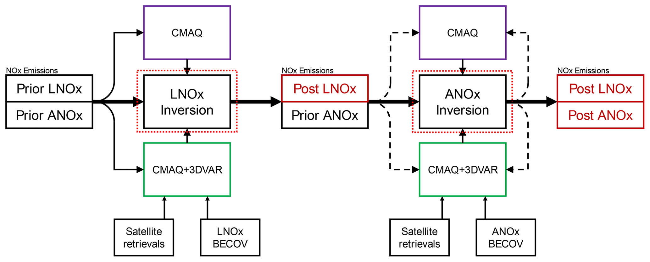
Figure 1NOx emissions inversion framework. Lightning NOx (LNOx) emissions are updated in the first step. Then, anthropogenic NOx (ANOx) emissions are updated iteratively. CMAQ boxes represent air quality simulations without chemical data assimilation, and CMAQ+3DVAR boxes represent air quality model simulations with chemical data assimilation. Satellite NO2 retrievals and a background error covariance (BECOV) are inputs to the chemical data assimilation, described in Sect. 2.3. Red dotted lines around the inversion boxes correspond to the red dotted lines in Fig. 3, which details the inversion algorithm. Dashed black emissions input lines around the ANOx inversion represent the iterative process. Iteration and convergence criteria are described in Sect. 2.6.
2.1 Satellite data
We use NO2 tropospheric column observations from the National Aeronautics and Space Administration's (NASA's) OMI and from the Royal Netherlands Meteorological Institute's (KNMI's) TROPOMI instruments in the inversion framework. TROPOMI was launched in October 2017 and provides 7.2×3.6 km2 resolution NO2 retrievals, upgraded to 5.6×3.6 km2 resolution in August 2019 (Van Geffen et al., 2020; Veefkind et al., 2012). TROPOMI's sun-synchronous polar orbit crosses the Equator at approximately 13:30 local time (LT), allowing the instrument to achieve global coverage in one day. We assimilate the Level-2 tropospheric slant column retrieved from NASA's Earth Science Data Systems program (https://www.earthdata.nasa.gov/, last access: 9 December 2022). The data product is described in the Algorithm and Theoretical Basis Document (ATBD) for TROPOMI NO2 (Van Geffen et al., 2019). We only consider TROPOMI observations with a quality flag greater than 0.5 and a cloud fraction lower than 30 % in the assimilation, following data product recommendations (Eskes et al., 2019). We use the latest publicly available versions of the TROPOMI retrieval for 2019 (versions 1.2.2 to 1.3.2) at the time of the analysis. Version 1.3 introduced updates to cloud processing that decreased noisy hotspots and broadened the range of acceptable air mass factors (Eskes et al., 2021). Information about the updates applied in each version and the dates on which updates were applied is given in Eskes et al. (2021). A research version with an updated retrieval applied to 2019 observations has been developed (Van Geffen et al., 2022) but was not yet standard and was not available at the time of this analysis. We discuss the impact of these latest updates in Sect. 3.3.
OMI, on board the Aura satellite launched in 2004, provides tropospheric NO2 vertical and slant column retrievals with a resolution of 13×24 km2 near nadir in a sun-synchronous polar orbit, with a local Equator crossing time of 13:45 LT. Global coverage is achieved in 2 d. We use the NASA Goddard Space Flight Center (GSFC) Level-2 NO2 product (Krotkov et al., 2019b). OMI was impacted by a row anomaly beginning in 2008, reducing the number of usable pixels in the OMI retrieval (Boersma et al., 2018). We include only pixels with a cloud fraction lower than 30 % and a summary quality flag of 0. Detailed information about the NO2 data product is included in the OMI ATBD (Chance, 2002) and in Krotkov et al. (2019a).
A low bias has been noted in the versions of TROPOMI NO2 used for this study (Judd et al., 2020; Verhoelst et al., 2021). Although TROPOMI NO2 retrievals from 2019 have been reprocessed with retrieval version 2.3.1, resulting in an improvement of the bias (Eskes et al., 2021), these reprocessed datasets were not yet available at the time this analysis was conducted. Figure 2 compares TROPOMI and OMI tropospheric vertical column densities (VCDs) for 2019, regridded to the CMAQ grid used. For the VCDs shown in the figure, we remove the effect of the assumed vertical profile of NO2 from the original satellite product by recalculating the VCDs with the NO2 vertical profile simulated by CMAQ. In the results, we discuss the low bias in TROPOMI data and explore its impact on emissions inversions.
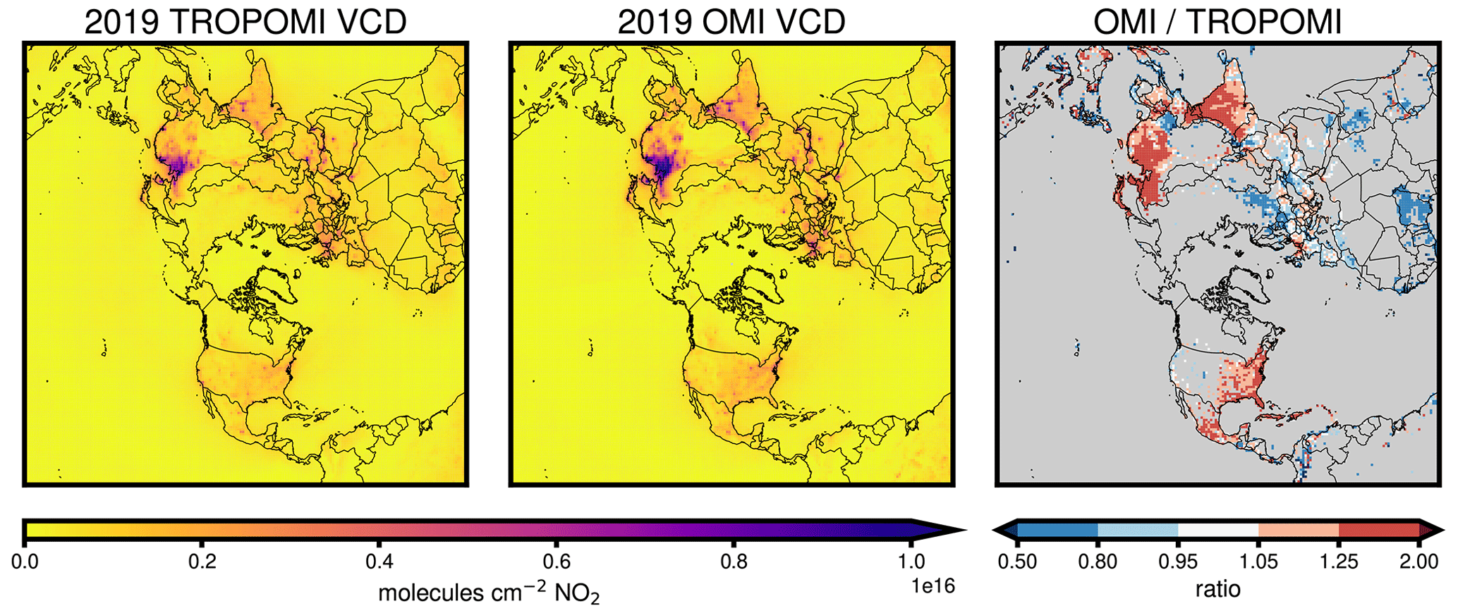
Figure 22019 annual average TROPOMI and OMI vertical NO2 vertical column densities, with CMAQ NO2 profiles applied, and the ratio between them. Column density ratios are only shown for the grid cells where NOx emissions updates are applied in the emissions inversion.
2.2 Hemispheric air quality modeling
Model simulations in the inversion framework were completed for January–December 2019 using CMAQ v5.3.2 (Appel et al., 2021; U.S. EPA Office of Research and Development, 2020). CMAQ has been used to simulate air quality over the Northern Hemisphere and has been shown to adequately capture chemical composition against observations (Mathur et al., 2017). Model inputs and satellite observations are summarized in Table 1. Simulations, designed to capture continental-scale pollutant transport, cover the Northern Hemisphere with 108 km horizontal grid spacing and a 44-layer vertical structure reaching 50 hPa (Mathur et al., 2017). The simulations use version CB6r3 of the Carbon Bond 6 chemical mechanism (Luecken et al., 2019), the AERO7 aerosol module (Xu et al., 2018) and updated halogen chemistry (Kang et al., 2021). Anthropogenic emissions are modeled using representative day-of-week emissions that change month to month. Representative-day emissions are created by averaging data from the prior emissions inventory on a day-of-week basis by month. For each day of the week and each month, there is a unique hourly emissions file that is used for every matching day of the week in that month. As a result, diurnal and weekly patterns are captured in the emissions, while daily variations that are specific to the prior emissions inventory year are averaged. The prior emissions inventory relies on the best available emissions data at the time of the study. Anthropogenic emissions for North America are from the U.S. Environmental Protection Agency's (EPA) 2017 National Emissions Inventory (NEI) modeling platform (Adams, 2020). Emissions in China are for the year 2015 (Zhao et al., 2018), and emissions for the rest of the hemisphere are based on the Hemispheric Transport of Air Pollution (HTAP) version 2, projected from their original 2010 date to 2014, with scaling factors from the Community Emissions Data System (CEDS). To initialize the 2019 prior and posterior simulations and to reduce the impact of chemical initial conditions on the results, we use a 1-year spin-up period not considered for the analyses. CMAQ model runs are driven by meteorology from a retrospective hemispheric simulation using the Weather Research and Forecasting (WRF) model (Skamarock et al., 2008) version 4.1.1, configured following Mathur et al. (2017) and Xing et al. (2015).
Table 1Prior emissions and model inputs.

* GEIA – Global Emissions Initiative; FINN – Fire Inventory from NCAR; CAMS – Community Atmosphere Modeling System; MEGAN – Model of Emissions of Gases and Aerosols from Nature
2.3 Chemical data assimilation in CMAQ
We adjust modeled NO2 concentrations using satellite observations by coupling the CMAQ model to a data assimilation model, the National Centers for Environmental Prediction (NCEP) Gridpoint Statistical Interpolation (GSI) program version 3.3 (Shao et al., 2016). GSI performs 3D variational (3DVAR) data assimilation by minimizing the cost function, J:
where y is the observation innovation , x is the analysis increment , xa is the analysis field (NO2 concentration after application of chemical data assimilation), xb is the model background (the simulated NO2 concentration before application of chemical data assimilation), yo is the satellite observations, B is the background error covariance matrix, R is the observation error matrix, and H is the observation operator. To compute the difference between the model column (xb) and the satellite column (yo), the observation operator H is applied, which transforms the model background to the form of the satellite observations. For TROPOMI data, the averaging kernel is first converted to scattering weights as
where A(z) is the vertically resolved TROPOMI averaging kernel for level z, Mtotal is the air mass factor provided with the satellite data, and w(z) is the vertically resolved scattering weights. Scattering weights accompany the OMI NO2 data product, so this step is not needed to assimilate OMI data. Scattering weights are then applied to compute the model slant column as
where is the model partial vertical column in the troposphere, interpolated to the satellite grid, and is the model tropospheric slant column density (SCD). The difference between the modeled and observed slant columns, or the observation innovation y in Eq. (1), is estimated as
where is the analysis increment, is the satellite tropospheric VCD, and Mtrop is the tropospheric air mass factor, distributed with the satellite data. We eliminate the influence of the a priori satellite vertical profile by computing the analysis increment with the modeled and observed SCD, which, unlike the VCD, does not rely on the a priori vertical NO2 profile assumed by the satellite.
We compute B using the Generalized Background Error covariance matrix model (GENBE v2.0) (Descombes et al., 2015), which models background errors by comparing a free-running simulation and a simulation with either lightning or anthropogenic NOx emissions perturbed. We use GENBE with the prior simulation and a simulation with a uniform −15 % perturbation to LNOx to create three-dimensional background errors in the upper troposphere for the LNOx assimilation. After updating LNOx emissions (as described in Sect. 2.5), we create three-dimensional background errors in the boundary layer for the anthropogenic NOx assimilation by using GENBE with the LNOx posterior simulation and a simulation with a −15 % perturbation to surface anthropogenic NOx emissions. Observation error R is provided with the satellite data.
Online coupling between GSI and CMAQ was developed in this study to perform the assimilation. At each model time step in which a satellite observation is available, the CMAQ model simulation is paused, and 3DVAR assimilation is performed. The CMAQ model state at that time step is used as xb. After assimilation using 3DVAR within GSI, CMAQ returns to a free-running mode, and the new model state, x, is updated to more closely match the satellite observation. The difference in the monthly average NO2 VCDs from the assimilation and no-assimilation runs is used in the inversion as ΔΩ.
2.4 Finite-difference mass-balance inversion
In the inversion framework developed, we iterate the approach of Lamsal et al. (2011). The FDMB process as applied here is summarized in Fig. 3. In the past, this approach has been used by directly comparing model and satellite columns (e.g., Itahashi et al., 2019; Cooper et al., 2017; Lamsal et al., 2011). We modify the approach by first updating model concentrations with assimilation of satellite observations and then updating the emissions using the difference between the modeled VCD with and without assimilated satellite information. All updates are performed on a monthly average basis.
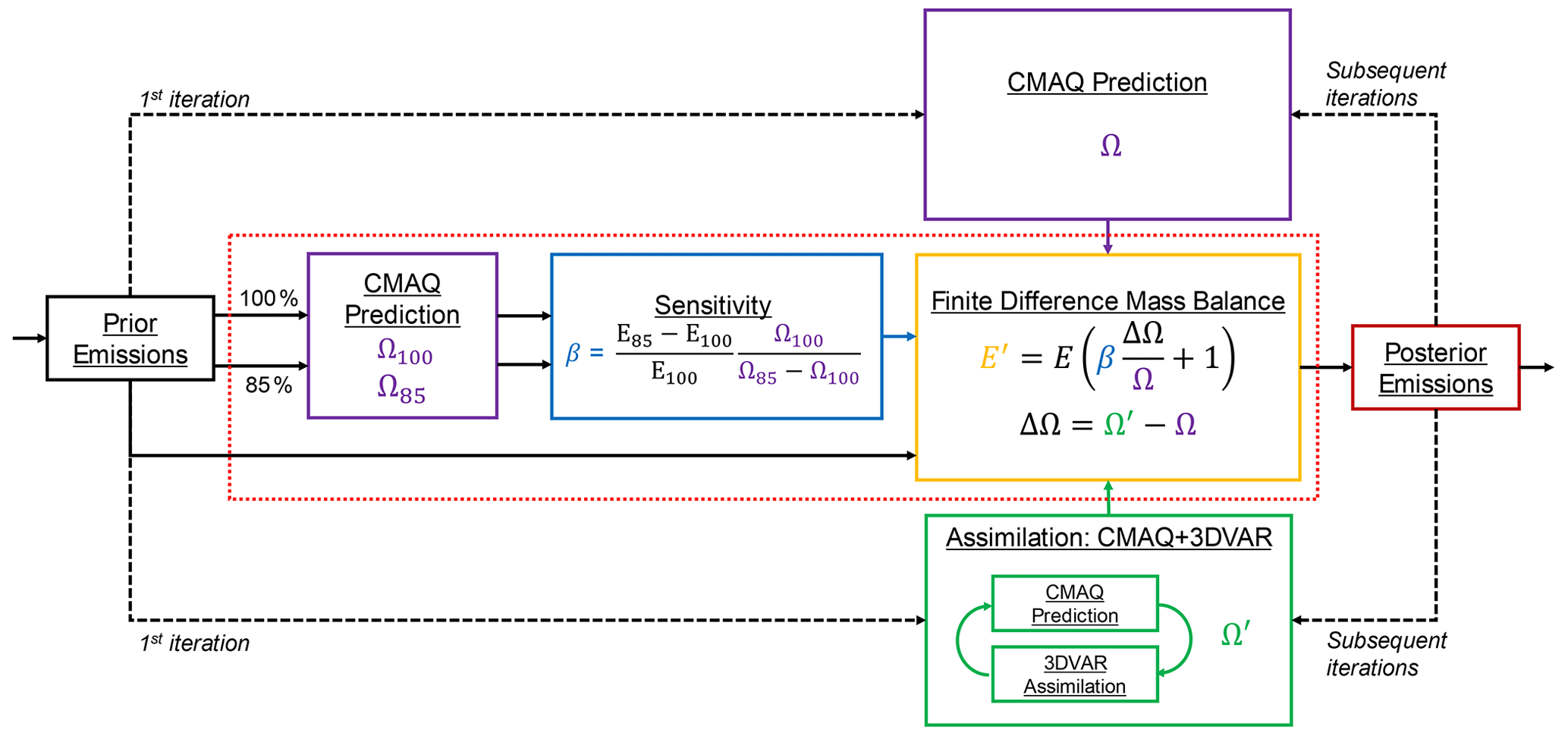
Figure 3FDMB inversion. The red dashed line corresponds to the red dashed lines in Fig. 1, and the processes inside show additional details of the FDMB inversion. In this framework, the prior emissions (black box on the far left) are input to the CMAQ model. CMAQ simulations are performed with unperturbed prior emissions (100 % arrow and E100) and prior emissions with a −15 % perturbation (85 % arrow and E85). The resulting modeled VCDs are Ω100 and Ω85, respectively. These VCDs are used to compute the sensitivity, β (blue box). New emissions totals are calculated with FDMB (yellow box), using β, NO2 VCD from a CMAQ simulation without assimilation (Ω), and NO2 VCD from a CMAQ simulation with assimilation (Ω′). When iteration is used, the posterior emissions from the previous iteration are used as input to the CMAQ model to simulate new VCDs, Ω and Ω′.
In FDMB, following Lamsal et al. (2011), emissions changes are inferred through the relationship
where ΔE is the inferred NOx emissions change, E is the NOx emissions prior, Ω is the model simulated NO2 VCD without chemical data assimilation, and is the monthly average difference between the model simulated tropospheric NO2 VCD with (Ωassim) and without (Ω) chemical data assimilation. β is a unitless scaling parameter, the Jacobian, that linearly relates NO2 VCD changes to NOx emissions changes. β is calculated through finite differencing as
where E′ is perturbed NOx emissions, ΩE is the tropospheric NO2 VCD simulated with model emissions E, and is the tropospheric NO2 VCD simulated with model emissions E′. To estimate β, we use the same −15 % perturbation used to create background errors B in the boundary layer. Cooper et al. (2017) found that using perturbations ranging from 5 % to 20 % to calculate β changed posterior emissions estimates by less than 2 % globally.
2.5 Inverse modeling NOx emissions
In our framework, LNOx emissions are updated first, separately from anthropogenic emissions. Due to the satellite instruments' sensitivity to NO2 in the upper atmosphere (e.g., Eskes and Boersma, 2003), small model biases there can influence the total column comparison and adversely impact the anthropogenic emissions adjustment. By updating LNOx emissions, we aim to decrease this bias and its impact on the ANOx inversion. We compute the scaling parameter for lightning emissions, , using the −15 % LNOx perturbation simulations applied to create background errors for the upper troposphere. We then assimilate satellite NO2 observations using the background errors for the upper troposphere and apply in a single inversion iteration using the full tropospheric VCD to compute spatially varying LNOx adjustment factors. Updates to LNOx are calculated using monthly averages.
After LNOx emissions are updated, ANOx emissions are updated by iteratively applying an FDMB inversion independently for each month in 2019. Iterating the FDMB has been shown to improve emissions estimates compared to a single FDMB application (Cooper et al., 2017). In the FDMB iteration, each update to the emissions serves as the prior emissions for the subsequent iteration (represented as black dashed lines in Fig. 1). The number of iterations is determined based on the synthetic observation experiment described in Sect. 2.6. β is held constant during all ANOx inversion iterations and is not recalculated each time to prevent instability in β as changes in the column become smaller with subsequent iterations. In the ANOx emissions inversion, we only consider grid cells in which local anthropogenic NOx emissions likely contribute significantly to the satellite-observed NO2 column by only including grid cells in which anthropogenic NOx emissions comprise at least 50 % of total NOx emissions, following Lamsal et al. (2011); population density is greater than 15 000 people km−2 (CIESIN, 2018); modeled cloud cover is less than 30 %; and the local time is 13:00 or 14:00 (OMI and TROPOMI overpass times). Only emissions in grid cells meeting these criteria are adjusted. Table S1 in the Supplement describes each simulation performed for the LNOx and ANOx inversions.
The FDMB method assumes that emissions impacts are local (i.e., emissions in one grid cell do not affect VCD amounts in neighboring grid cells). This assumption is most valid when NOx lifetime is shorter than NOx transport time to neighboring grid cells, which is typical near the surface in coarse-resolution models (Martin et al., 2003), such as the one used in this study. However, the assumption is less realistic at finer resolutions and in the upper troposphere, where the lifetime of NO2 is longer than at the surface and where NO2 concentrations are not directly impacted by coincident near-surface emissions. Even at coarse resolutions (e.g., 100 km grid spacing), emissions-smearing effects, which occur when the FDMB assumption of local emissions effects is incorrect and emissions are inappropriately adjusted, can appear due to NOx transport, reservoir species, and chemical feedbacks (Turner et al., 2012; Cooper et al., 2017). Traditional FDMB, which directly compares modeled and remotely sensed columns, cannot address this effect. Assimilating the satellite VCD introduces an additional complication. The horizontal length scales (on the order of several hundreds of kilometers) used in the background error extend beyond the grid cell horizontal dimensions (nominally 108 km) in the middle and upper troposphere; as a result, NO2 changes introduced by assimilation (ΔΩ) do not have a local relationship with surface emissions directly below. In our work, assimilating the observed column information instead of directly comparing modeled and satellite-retrieved VCDs allows the analysis to be restricted to the lower troposphere, mitigating both the misallocation errors of FDMB and the effect of horizontal length scales extending beyond the grid cell dimension. To that end, we limit the anthropogenic emissions analysis to the lowest 20 model layers, which is nominal from the ground to ∼720 hPa over non-mountainous terrain in the summer, and use that partial column to calculate ΔΩ in the FDMB inversion. ΔΩ for a single month above and below the threshold is illustrated in Fig. S1 in the Supplement. By applying this cutoff, we focus the inversion on surface anthropogenic NOx.
2.6 Inversion system testing
We conduct a synthetic observation experiment to evaluate the ability of the inversion system to constrain emissions to a known perturbation. Artificial NO2 observations were generated from CMAQ simulations with unperturbed emissions and NOx emissions reduced by 15 %. As expected, assimilating the synthetic observations derived from a simulation with unperturbed emissions results in an analysis increment of zero. The results of an iterative emissions inversion based on the synthetic observations derived from the simulation with perturbed emissions are shown in Fig. S2. Across Northern Hemisphere regions, the normalized mean error (NME) relative to the known perturbed emissions and the rate at which it changes decrease with subsequent iterations. The NME is minimized after seven to nine iterations, depending on the region. In all subsequent results, emissions inferences made with eight iterations of the inversion system are shown and analyzed. Convergence of the inversion in different global regions adds confidence to the system's ability to constrain real-world emissions.
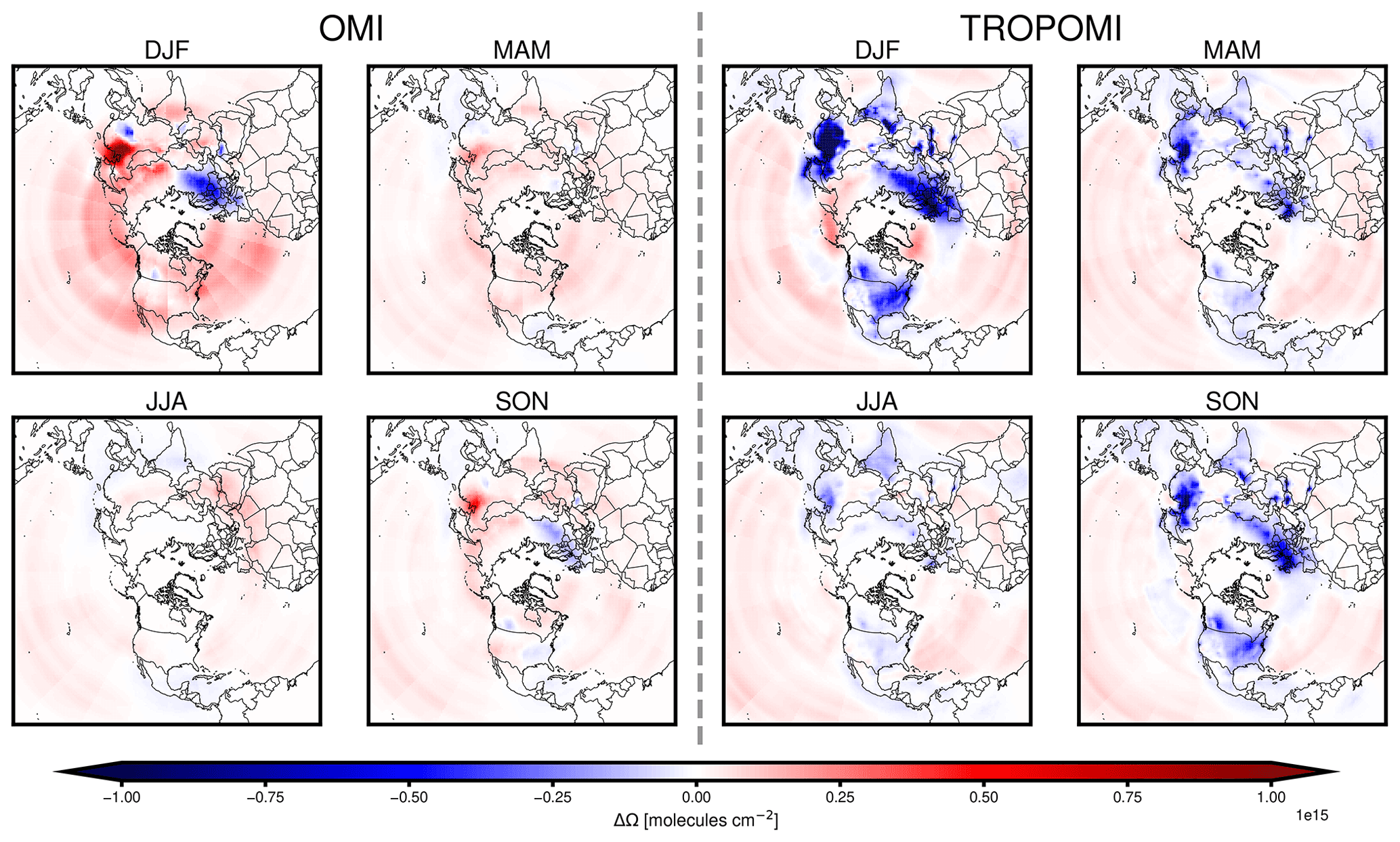
Figure 4Seasonal NO2 VCD change (ΔΩ) from CMAQ simulation using prior emissions after assimilating OMI or TROPOMI tropospheric NO2 observations and modeling atmospheric composition with prior NOx emissions. ΔΩ shown for winter (DJF), spring (MAM), summer (JJA), and fall (SON).
3.1 Lightning NOx emissions updates
Assimilation of retrievals from either satellite increases LNOx emissions across all seasons, relative to the prior emissions (monthly climatology from GEIA), with the largest changes occurring during the summer (Figs. S3 and S4). Applying 2019 OMI data increases total LNOx emissions in 2019 by 20 % over the GEIA climatology, while assimilation of TROPOMI data increases LNOx emissions by 24 %. The emissions increases inferred by both satellite products are driven by NO2 increases in the mid and upper troposphere due to assimilation, with changes near the surface being negligible in comparison. Increases in background areas with small NO2 column totals and subsequent LNOx increases in these areas suggest a low bias in modeled background NO2 relative to observations from both satellites. A low bias agrees with the findings reported by other model and satellite NO2 comparisons (Silvern et al., 2019; Qu et al., 2021; Goldberg et al., 2017). The LNOx emissions adjustments inferred here decrease the differences between modeled and satellite-derived NO2 in the upper troposphere and decrease the bias that differences in the upper troposphere can introduce to the subsequent ANOx inversion.
3.2 Impact of assimilation on modeled NO2 vertical column density
Figure 4 shows the change to CMAQ-modeled tropospheric VCD, (ΔΩ) caused by assimilating NO2 observations from OMI or TROPOMI with background errors for the boundary layer, before applying any emissions adjustments. In Fig. 4 and throughout the results, ΔΩ reflects differences near the surface (as described in Sect. 2.5). Assimilating OMI NO2 data generally increases modeled NO2 columns near populated areas in China, India, and the US. In contrast, assimilating TROPOMI NO2 data decreases modeled NO2 columns more widely across the Northern Hemisphere. The changes brought about by assimilating satellite data are larger during the winter and fall and smaller in the spring and summer, when NOx lifetime is shortest and when NO2 columns are smaller. During the winter in northeast China, where the assimilation impacts are most apparent, the seasonal average change due to assimilation reaches 1.8×10¹⁵ molec. cm−2 for OMI and molec. cm−2 for TROPOMI. The direction of ΔΩ after assimilation of OMI data is more heterogeneous and shows a stronger seasonality, while ΔΩ based on assimilating TROPOMI data is consistently negative. Over Europe, ΔΩ after assimilating OMI observations is close to zero in warm months and negative in colder seasons. Assimilating satellite-observed NO2 increases the NO2 levels modeled over the ocean and less-populous areas, such as the Sahara, with low NOx emissions and small NO2 column amounts.
Over polluted areas, the direction of ΔΩ for the TROPOMI or OMI data assimilations tends to differ. This discrepancy is likely due to the low bias in TROPOMI-derived tropospheric NO2 columns, which has been reported to be approximately 10 % over the US, Europe, and India, and greater than 20 % over China when compared with the OMI Quality Assurance for Essential Climate Variables (QA4ECV) retrieval (Van Geffen et al., 2022; Verhoelst et al., 2021; C. J. Wang et al., 2020; Li et al., 2021). Over background areas, the analysis increments that result from assimilation of observations from both satellites generally agree. The consistency suggests a low bias in modeled background NO2 concentrations and also agrees with the low bias in CMAQ-modeled free-tropospheric NO2 reported by Goldberg et al. (2017). Such a bias can contribute to the positive analysis increment over background areas. However, NO2 columns observed in these regions may be smaller than the retrieval accuracy of 0.7×10¹⁵ molec. cm−2 (Van Geffen et al., 2019), reducing confidence in the analysis increment at these locations. In the anthropogenic emissions inversion, our filtering criteria exclude background areas which are more likely to have low VCD amounts.
3.3 Emissions inversion
Season-average β values, relating NO2 vertical column differences to anthropogenic near-surface NOx emissions updates, are shown in Fig. S5. Based on our criteria for grid cell inclusion in the inversion, described in Sect. 2.5, we consider 13 % of the grid cells in the domain, which represent 88 % of prior anthropogenic NOx emissions. Seasonal domain-average values range from 1.33 to 1.66 and are lower in the winter and higher in the summer. A β value less than 1.0 results in an emissions update that is smaller than the VCD change, while a β greater than 1.0 has the opposite effect. β tends to be less than 1.0 in polluted regions during colder months and larger during warmer months and in less-polluted regions, although many grid cells which are less polluted are not considered in the analysis. The scaling factors are smallest over China and larger over the US, India, Mexico, and Europe. The differences among regions stem from local differences in NOx lifetime and transport. In Indonesia and sub-Saharan Africa, lower emissions and a small response from tropospheric VCD to anthropogenic emissions perturbations can lead to large β values. To prevent overly large or small β values, we constrain the factor to between 0.1 and 10, following Cooper et al. (2017). Scaling factors estimated here are larger than the 1.16 global-average previously reported by Lamsal et al. (2011). However, in Lamsal et al. (2011), modeled NO2 vertical columns were sampled at the morning SCanning Imaging Absorption spectroMeter for Atmospheric CHartographY (SCIAMACHY) overpass time rather than at the afternoon OMI or TROPOMI overpass times; β tended to be closer to 1.0 during the morning in regions with high NOx emissions (Li and Wang, 2019). Li and Wang (2019) show that, over rural regions with lower NOx concentrations, β is larger at the OMI or TROPOMI overpass window than at the SCIAMACHY overpass window, suggesting that a larger overall β for analyses based on OMI or TROPOMI products should be expected. Additionally, NOx emissions have decreased considerably in several regions of the Northern Hemisphere, including the US (Tong et al., 2015) and China (Miyazaki et al., 2017), after the Lamsal (2011) study was conducted, which has changed the sensitivity of NO2 VCDs to NOx emissions (Qu et al., 2021; Silvern et al., 2019).
Annual bottom-up prior ANOx emissions estimates are shown in Fig. 5. Season-average ANOx emissions inferences from the inversions based on OMI and TROPOMI observations are shown in Fig. 6. The use of OMI observations generally tends to increase emissions in most industrialized nations outside of Europe. NOx emissions increases driven by OMI observations are largest in winter and spring and smaller, or slightly decreased, in summer and fall. In contrast, the use of TROPOMI retrievals tends to drive a decrease in NOx emissions across all seasons and continents, with the largest impacts in the summer and the smallest in the spring. The largest emissions changes based on both OMI and TROPOMI retrievals are in northeast China during the winter. Over India, OMI-inferred changes are concentrated in central India, where prior emissions are lower, while the largest changes inferred from TROPOMI are in the northern, eastern, and southern zones, where prior emissions are highest. Relative NOx emissions changes driven by TROPOMI observations tend to be small over dense urban areas, with more uniform decreases over cells with lower emissions.
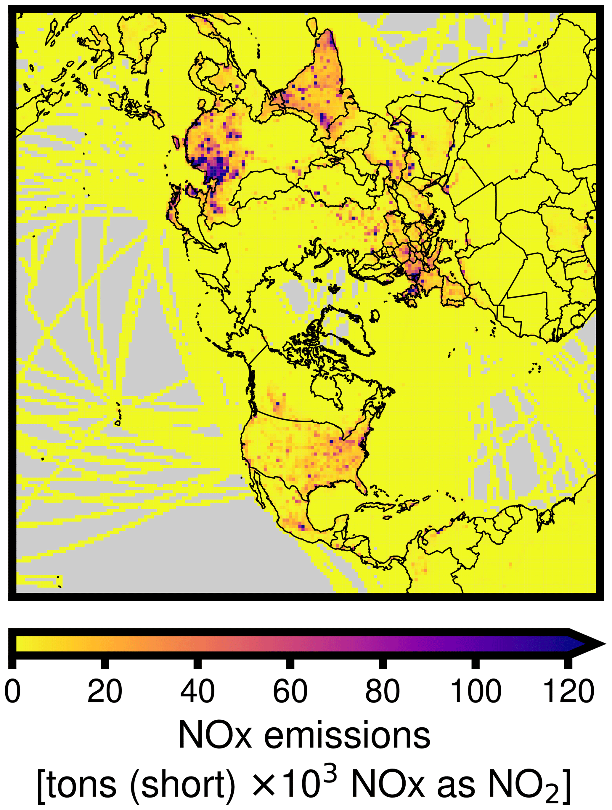
Figure 52019 prior anthropogenic NOx emissions totals. Data sources are described in Table 1.
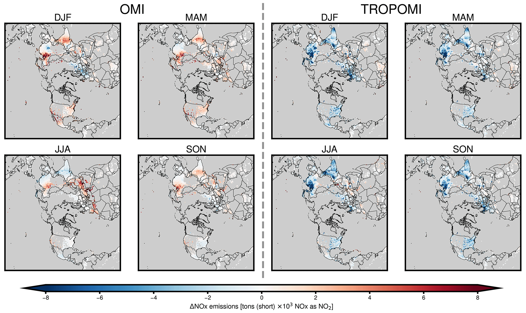
Figure 6Season-average NOx emissions changes from inverse modeling updates based on OMI and TROPOMI observations. Emissions changes are shown for winter (DJF), spring (MAM), summer (JJA), and fall (SON).
ANOx emissions totals and inferred changes are explored for China, India, Europe, Mexico, and the US (Fig. 7). We also show 2019 NOx emissions totals from the Copernicus Atmosphere Monitoring Service's (CAMS's) bottom-up emissions inventory (Granier et al., 2019) and from the NASA Tropospheric Chemical Reanalysis products 2 (TCR-2) satellite-inferred inventory (Miyazaki et al., 2019, 2020). TCR-2 top-down NOx emissions are constrained using satellite observations of NO2, CO, O3, and SO2 at a resolution of and are further described in Miyazaki et al. (2017). CAMS anthropogenic NOx emissions are based on the Emissions Database for Global Atmospheric Research (EDGAR version 5.3) estimates for 2015 (Crippa et al., 2020), projected to 2019 using CEDS scaling factors, and are provided at . Both datasets provide monthly anthropogenic NOx totals. Except for Europe, assimilation toward OMI retrievals increases annual emissions totals in the regions analyzed, while using TROPOMI retrievals decreases them. TCR-2 NOx emissions estimates are larger than the prior emissions used by our inverse modeling framework, except for India, while CAMS totals are lower than the prior emissions estimates and are similar to TROPOMI inferred emissions. Across the regions considered, TROPOMI infers an average annual decrease of −33 % in NOx emissions from the regions, while OMI infers a +9 % increase. In Europe, the only region where the sign of the inferred changes match, the use of OMI retrievals results in a −1 % change, while applying TROPOMI observations leads to a −36 % decrease in NOx emissions. The largest total changes are inferred in the highest-emitting region, China, while the greatest relative changes, −41 % inferred with TROPOMI, are for India, where emissions are highly uncertain. Changes inferred with OMI observations over the US are greater than 1200×103 short tons NOx as NO2 per year but smaller than the difference between our prior US emissions estimates and TCR-2 or CAMS estimates. A change of short tons NOx as NO2 emitted annually in the US, as inferred by TROPOMI, over 30 % of the prior emissions differs significantly from National Emissions Inventory estimates but leads to a total close to that of the 2019 CAMS inventory.
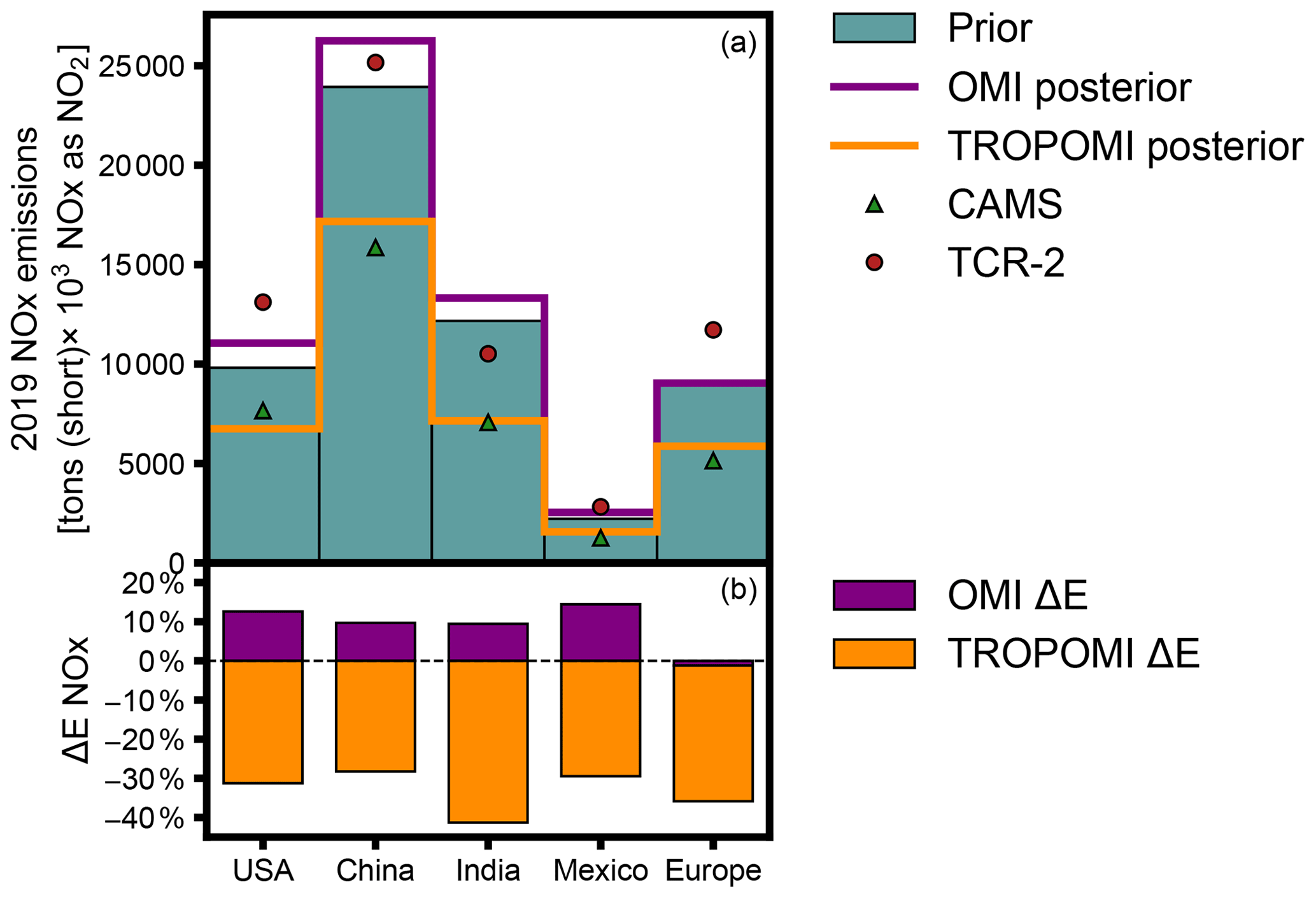
Figure 7Prior and satellite-inferred 2019 anthropogenic NOx emissions in select global regions. Plot (a) shows total emissions (as NO2) from prior emissions estimates, inference with OMI or TROPOMI observations (OMI and TROPOMI posterior), and CAMS or TCR-2 inventories in the US, China, India, Mexico, and Europe. Plot (b) shows the percent change (ΔENOx) inferred with OMI or TROPOMI data, relative to prior emissions estimates, for each region.
Across the months simulated, inferences using OMI retrievals consistently lead to higher NOx emissions than using TROPOMI retrievals. Figure 8 shows monthly NOx emissions totals and inferred changes for several global regions. The magnitude of changes is generally smallest in summer months and largest in winter months for both OMI- and TROPOMI-inferred emissions. Monthly prior emissions totals lay between the OMI and TROPOMI inferences, except for summertime emissions in India and Mexico, where both satellite inferences decrease NOx emissions. Over Europe, both satellite products infer a decrease during the winter, although fewer valid satellite pixels due to snow cover at high latitudes and longer winter NO2 atmospheric lifetimes may influence the inference.
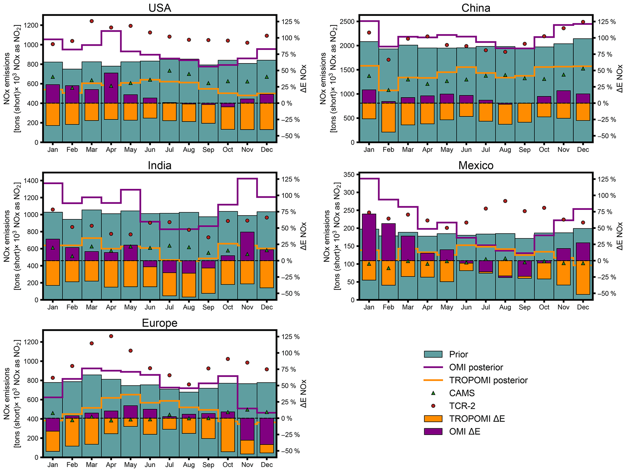
Figure 8Monthly prior and satellite-inferred anthropogenic NOx emissions in 2019 in select global regions. Total monthly emissions (as NO2) from prior emissions estimates, inference with OMI or TROPOMI observations (OMI and TROPOMI posterior), and CAMS or TCR-2 inventories in the US, China, India, Mexico, and Europe are shown. Percent changes (ΔENOx) inferred with OMI or TROPOMI data, relative to prior emissions estimates, for each region are shown by the purple and orange bars.
Based on reported NOx emissions trends (McDuffie et al., 2020; U.S. EPA, 2022a), changes from the prior emissions inventory (Table 1) to 2019 are expected. Relative to the prior emissions, significant decreases in NOx emissions in China, estimated for 2015 in the prior inventory, and smaller reductions in Europe and North America, reported for 2014 and 2017 in the prior inventory, respectively, should be anticipated. TROPOMI-inferred emissions reflect the direction anticipated for these changes but with larger than expected magnitudes. For example, the 28 % decrease in anthropogenic NOx emissions over China between 2015 and 2019 inferred from the TROPOMI observations is substantially larger than the 8 % decrease estimated between 2015 and 2017 by the Community Emissions Data System (McDuffie et al., 2020). Bottom-up estimates indicate that anthropogenic NOx emissions in the US have decreased through 2019 (U.S. EPA, 2022a). Although the direction of the emissions change inferred from TROPOMI agrees with the trend in bottom-up estimates, its magnitude is larger than expected. An underestimation of US emissions in winter in the prior inventory when compared with OMI inferences contrasts with field study results reporting no bias in northeastern US winter emissions estimates (Jaegle et al., 2018; Salmon et al., 2018). In India, bottom-up emissions inventories report sustained growth of NOx emissions (Kurokawa and Ohara, 2020; McDuffie et al., 2020), and NO2 levels observed by OMI have been increasing since 2005 (Goldberg et al., 2021; Cooper et al., 2022). The decrease in anthropogenic NOx emissions inferred by TROPOMI observations contrasts with these trends in bottom-up estimates and OMI observations.
The low bias known to affect TROPOMI NO2 observations influences the results of the emissions inversion, which targets grid cells with high emissions, likely leading to decreases in inferred emissions that are larger than expected. We conduct an inversion using the reprocessed TROPOMI NO2 version 2.3.1 (Van Geffen et al., 2022) to infer NOx emissions for January 2019 and find that the updated data increase the TROPOMI posterior inference by 17 % over the US and 4 % in China relative to version 1.2.2. While using the updated retrievals shrinks the gap between OMI- and TROPOMI-inferred emissions, it does not change the overall trend of smaller posterior emissions using TROPOMI NO2 (Figs. S10 and S11). The differences between emissions inferred by OMI and TROPOMI observations highlight the importance of ongoing efforts to harmonize OMI and TROPOMI NO2 retrieval algorithms, such as the NASA Multi-Decadal Nitrogen Dioxide and Derived Products from Satellites (MINDS) (Lamsal et al., 2020) and the QA4ECV (Boersma et al., 2017) datasets.
In addition to smearing effects, coarse-resolution models can artificially alter nonlinear NO2 chemistry, leading to biases in inferences of NOx emissions from satellite NO2 columns (Valin et al., 2011; Sekiya et al., 2021; Lamsal et al., 2011). Higher-resolution simulations can better resolve β and reduce biases caused by nonlinear chemistry. Additional errors in the emissions estimates may be associated with emissions from non-anthropogenic NOx sources. Although the emissions inversion targets anthropogenic sources only, changes in NO2 columns observed by the satellite instruments driven by natural NOx emissions processes may not be captured in the air quality model simulations and subsequently lead to biased anthropogenic emissions inferences (Li et al., 2021).
The emissions resulting from the inverse modeling framework are comparable to CAMS and TCR-2 2019 emissions estimates in several ways. In the US, China, and Europe, the magnitudes of ANOx emissions from OMI retrievals are comparable to TCR-2 NOx emissions estimates and exhibit similar monthly patterns. Annual NOx emissions inferred from OMI observations are also relatively similar to TCR-2 estimates for India and Mexico, although monthly emissions patterns differ. Unlike TCR-2 emissions estimates, which are also constrained by OMI NO2 observations, 2019 CAMS emissions estimates are projected from 2015 bottom-up data. However, CAMS estimates provide a representation of anticipated emissions trends. In all regions considered, CAMS NOx emissions estimates are close to the TROPOMI inference annual totals and lower than the prior emissions, OMI inferences, and TCR-2 estimates, potentially suggesting that global NOx emissions have not decreased as much as anticipated by the CAMS inventory projections.
3.4 Impacts of emissions updates on modeled NO2 and O3
We evaluate and compare the CMAQ simulations' ability to reproduce observed pollutant concentrations when driven with NOx emissions estimates from the prior inventory and with those derived by the inverse modeling framework. Figure 9 compares 2019 OMI and TROPOMI NO2 VCD retrievals with modeled NO2 VCDs using the prior emissions with no updates, LNOx emissions updates, and LNOx and ANOx emissions updates. Satellite-based LNOx emissions updates improve CMAQ model performance – correlation coefficient (R), normalized mean error (NME), and normalized mean bias (NMB) – when evaluated against tropospheric VCD retrievals, relative to model performance with the prior emissions. OMI-inferred ANOx emissions updates further improve CMAQ model performance evaluated against VCD retrievals, decreasing NMB from −20 % to −5 % and NME from 38 % to 28 %. Model performance is improved by using OMI data in the inverse modeling framework across all seasons (Figs. S6–S9). Although LNOx emissions updates derived from TROPOMI observations improve model bias and error relative to the CMAQ simulation using prior emissions estimates, TROPOMI-inferred anthropogenic emissions do not, except during summer months (Figs. 9 and S6–S9). The lack of significant improvements in CMAQ-simulated NO2 VCDs after applying the emissions inversion with TROPOMI NO2 retrievals prior to the version 2.3.1 update (Van Geffen et al., 2022) may be associated with changing chemical regimes that are not captured in the emissions inversion process.
Changes in modeled VCD due to assimilation and the emissions inferences calculated in the TROPOMI ANOx inversion exceed the emissions perturbation and VCD changes used to calculate β. For example, over the eastern US, the −15 % emissions perturbation used to calculate β leads to VCD changes of −15 % on average in winter, but assimilating TROPOMI retrievals leads to VCD changes (ΔΩ) of −19 % on average in the winter, with individual changes exceeding −30 %. Modeled NOx chemistry and NO2 vertical profiles after assimilating TROPOMI retrievals may be different than those used in the calculation of β. As a result, assimilating TROPOMI retrievals in the ANOx inversion may lead to modeled NO2 vertical profiles which are inconsistent with the precalculated β used in the FDMB relationship and to less reliable subsequent emissions inferences. In contrast, the magnitude of VCD changes due to assimilating OMI retrievals over the eastern US in winter is 8 %, well within the magnitude of the VCD changes used to precalculate β. This highlights the importance of applying a β sensitivity valid for the magnitude of anticipated emissions changes in FDMB inversions and the potential consequences of relying on satellite-derived retrievals with pre-existing biases in emissions inversions.
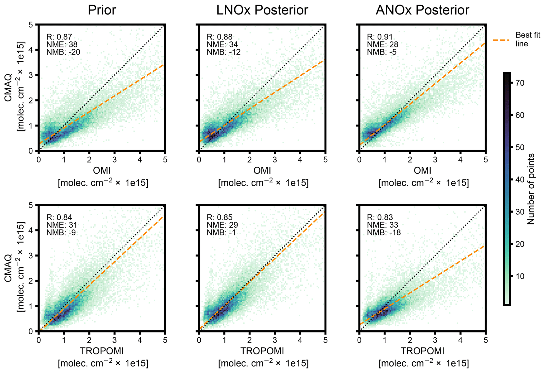
Figure 9Impact of NOx emissions updates on modeled NO2 VCDs. Plots compare 2019 season-average CMAQ-modeled NO2 VCD at each model grid cell in which NOx emissions were updated by the inverse modeling framework against OMI and TROPOMI tropospheric NO2 VCD retrievals averaged in each model grid cell. Modeled NO2 VCD using prior emissions (Prior), inferred LNOx emissions (LNOx posterior), and inferred lightning and anthropogenic NOx emissions (ANOx posterior) are each compared with NO2 VCD retrievals. Top-row plots compare retrievals and modeled VCD based on OMI observations, while bottom-row plots compare retrievals and modeled VCD based on TROPOMI observations. Linear regression line, correlation coefficient (R), normalized mean error (NME), and normalized mean bias (NMB), relative to tropospheric NO2 VCD retrievals, are shown for each CMAQ simulation.
Comparing CMAQ-modeled O3 to ozonesonde measurements from the World Ozone and Ultraviolet Radiation Data Centre (WOUDC) network shows the impacts updating LNOx emissions on simulated tropospheric O3 (Fig. 10). Above 300 hPa, the model is biased low, but neither update has a major impact on this bias. However, within the free troposphere, the effects of LNOx emissions updates are larger. LNOx satellite-inferred emissions from both satellites increase O3 and subsequently improve the model's low O3 bias across all seasons, with the strongest effect in the summer. This suggests a low background NO2 in our prior simulation, consistent with several studies demonstrating that models underestimate background NO2 (Goldberg et al., 2017; Qu et al., 2021; Silvern et al., 2019).
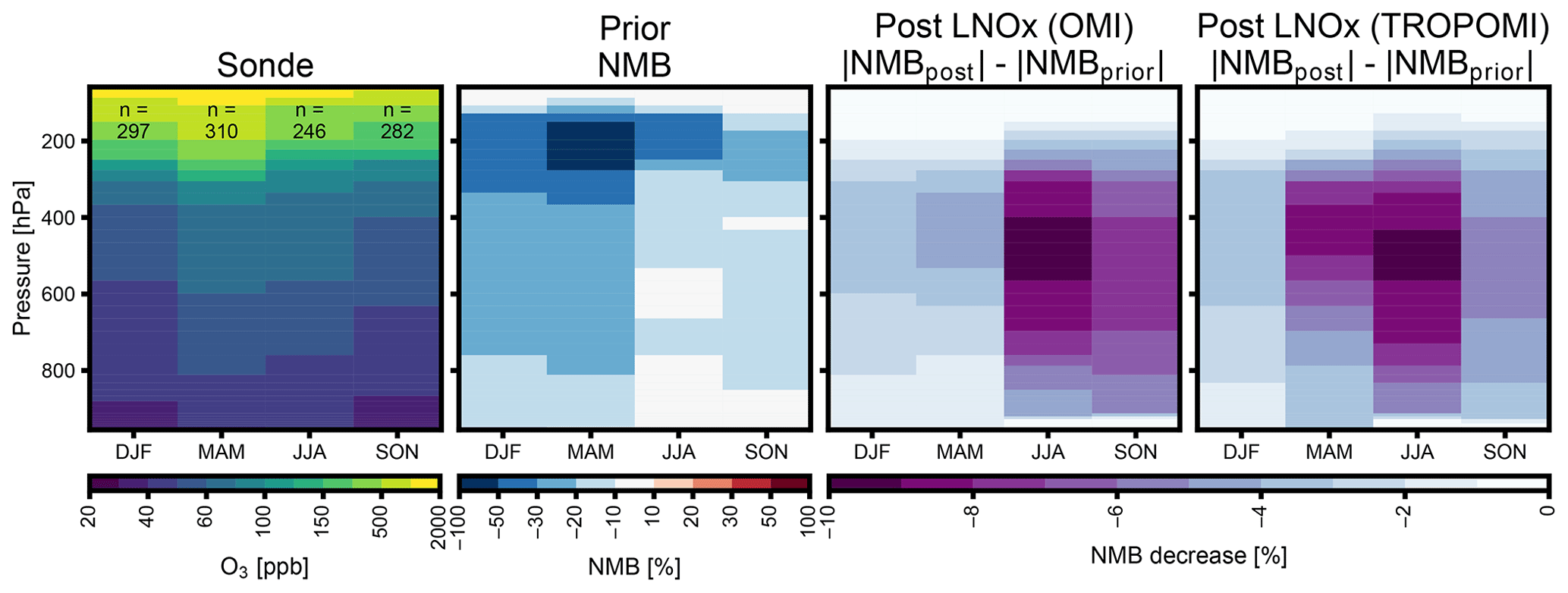
Figure 10Ozonesonde observations from the WOUDC network and impact of lightning emissions inferences on modeled ozone. Left plot shows sonde observations averaged in each season and total number of launches per season. The NMB is shown for the prior emissions simulation. Plots on the right show the decrease in the NMB, relative to the prior simulation for simulations, with LNOx emissions updated with OMI and TROPOMI data.
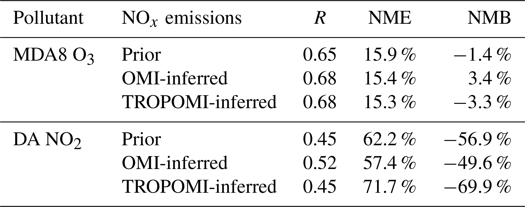
Comparisons of CMAQ-modeled NO2 and O3 concentrations with ground-level measurements highlight the challenges of reproducing local air quality with a coarse scale model but suggest potential to improve model performance with satellite-derived NOx emissions updates. Table 2 shows statistics evaluating modeled ground-level daily average NO2 and maximum 8 h O3 concentrations over the US against observations from 1218 monitoring sites in the Air Quality System (AQS) (U.S. EPA, 2022b), excluding near-road monitors for which the gridded NO2 fields are not representative. Statistics for each season are included in Tables S2 and S3. There is a significant low bias in CMAQ-predicted ground-level NO2 concentrations compared with monitoring site measurements, likely due to the model's coarse grid resolution and the aggregation of NO2 monitors within urban areas with high NOx emissions and large concentration gradients. CMAQ simulations at higher horizontal resolution do not show the same bias against NO2 surface observations (Toro et al., 2021). Agreement between modeled and observed ground-level NO2 concentrations is improved by using OMI-inferred NOx emissions compared with the prior emissions simulation, particularly during winter and spring months. Model performance evaluated against ground-level O3 measurements improves to a smaller extent with OMI-inferred NOx emissions during winter and spring months. The use of TROPOMI-inferred emissions has mixed impacts on CMAQ performance against observed ground-level NO2 and O3 concentrations, leading to limited gains in seasonal R and some seasonal biases and errors but also less agreement with observations for other seasonal statistics. In the US, the network of ground-based air quality observations is relatively large. However, in some regions where emissions uncertainties are expected to be especially high, ground-based observations are significantly limited and less accessible. Assessing the impact of emissions updated against ground-based observations in these regions, although a challenge, would provide further evaluation of the inversion framework in locations where satellite retrievals have the largest potential to provide important constraints to emissions estimates.
Table 2CMAQ model performance evaluated against daily average NO2 (DA NO2) and maximum 8 h O3 concentrations (MDA8 O3) observed in 2019 by AQS monitoring sites in the US. Near-road monitors are not considered. Statistics are shown for simulations using prior emissions (Prior), lightning and anthropogenic NOx emissions inferred with OMI data (OMI-inferred), and lightning and anthropogenic NOx emissions inferred with TROPOMI data (TROPOMI-inferred). Coefficient of determination (R), normalized mean error (NME), and normalized mean bias (NMB), relative to AQS observations, are estimated for each CMAQ simulation.
3.5 Impacts of emissions updates on long-range O3 transport
Global NOx emissions estimates affect model simulations of long-range air pollution transport. To explore these impacts, we examine the response of CMAQ-modeled trans-Pacific O3 to the inverse modeling framework's NOx emissions updates. Figure 11 shows season-average changes in simulated free-tropospheric O3 over the North Pacific Ocean resulting from the use of OMI- and TROPOMI-inferred ANOx emissions relative to the emissions simulation with LNOx emissions updated. As expected, the emissions inversions lead to O3 variations that follow NOx emissions changes inferred for each satellite's observations, with OMI inferences resulting in higher O3 concentrations and TROPOMI inferences resulting in lower O3 concentrations over the North Pacific Ocean. Season-average differences with respect to the prior emissions simulation are as large as +1.8 ppb in winter, using OMI-based updates, and −1.9 ppb in spring, using TROPOMI-based updates. Combined with trans-Pacific wind patterns, the effects of the NOx emissions inversions on modeled O3 suggest potential implications of uncertain Asian emissions estimates for US air quality management and emphasize the impacts of biases in satellite retrievals on inverse modeling systems.
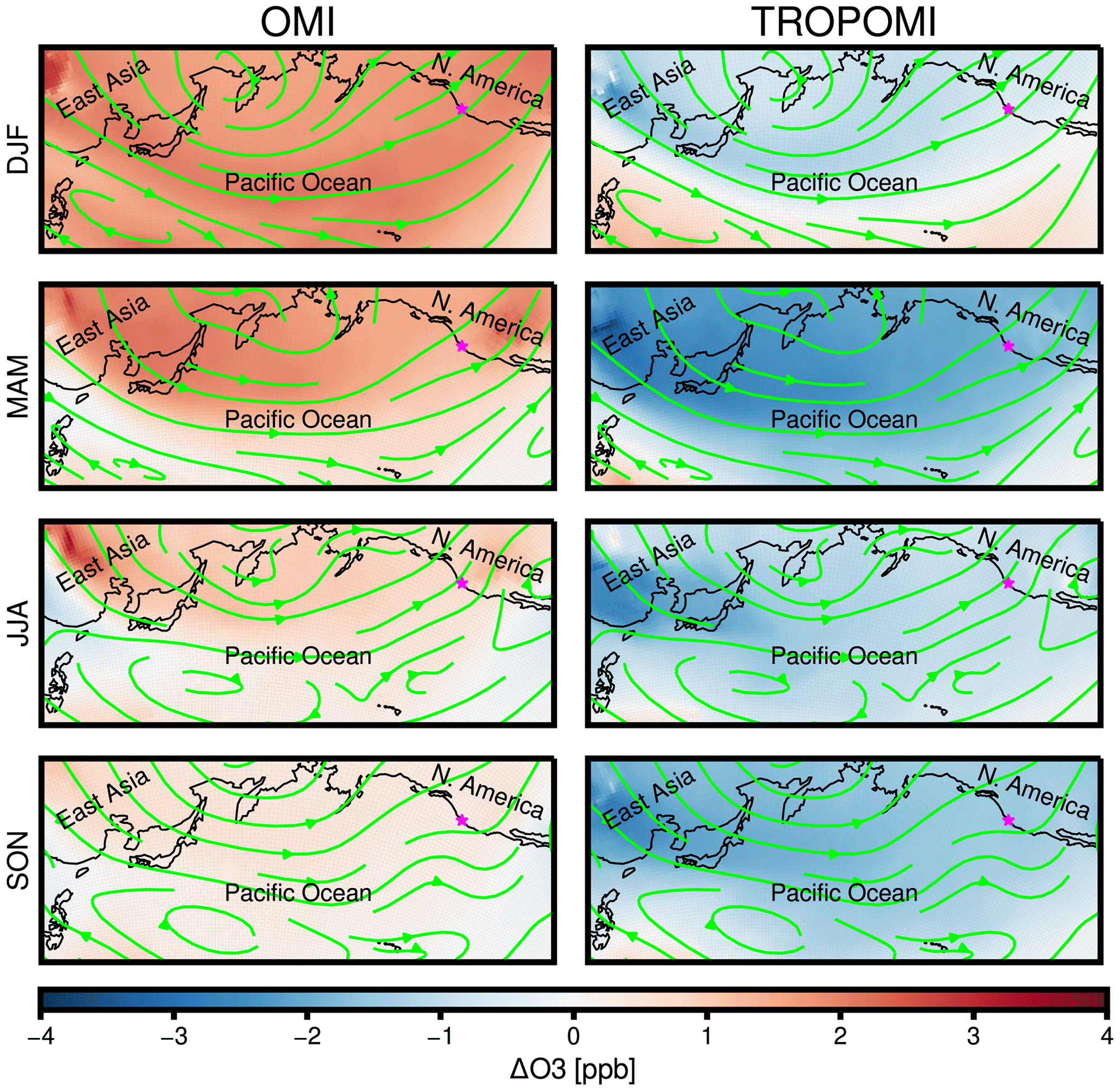
Figure 11Changes in 2019 season-average free-tropospheric O3 concentrations (averaged between 750 and 250 hPa) simulated over the North Pacific Ocean using lightning and anthropogenic NOx emissions inferred with OMI or TROPOMI observations, relative to simulations using prior ANOx emissions and updated LNOx emissions. Differences are shown for winter (DJF), spring (MAM), summer (JJA), and fall (SON). Arrows depict season-average free-tropospheric winds (750–250 hPa). Star marker indicates location of Trinidad Head, California.
At the Trinidad Head, California, a location where atmospheric composition is relatively unaffected by local emissions sources and is responsive to trans-Pacific pollution transport (Fig. 11), differences in modeled daily average free-tropospheric O3 concentrations can reach +5 or −3 ppb. Figure 12 compares CMAQ-modeled vertical O3 profiles to observations from 39 ozonesondes launched at Trinidad Head in 2019 (WOUDC, 2019). Relative to the CMAQ simulation using prior emissions, NOx emissions updates inferred from OMI and TROPOMI data can improve the model's ability to reproduce ozonesonde O3 distributions measured from the site, in particular during winter and spring, when the discrepancies between modeled and observed concentrations are largest. These impacts on modeled vertical O3 profiles are largely driven by changes the modeling framework's updates to lightning NOx emissions. The inferred LNOx increases from each satellite improve O3 biases, while subsequent anthropogenic updates have smaller impacts, suggesting that biases in O3 could be driven by background NO2 composition in the model and not solely by long-range transport resulting from anthropogenic emissions.
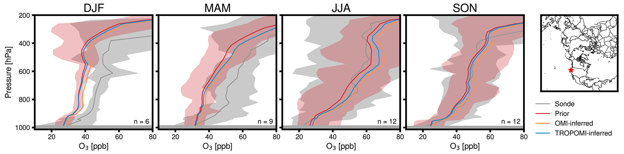
Figure 12Season-average vertical O3 concentration profiles modeled by CMAQ and measured by ozonesondes launched at Trinidad Head, California, in 2019. Vertical distributions are shown for simulations using prior emissions (Prior), lightning and anthropogenic NOx emissions inferred with OMI data (OMI-inferred), and lightning and anthropogenic NOx emissions inferred with TROPOMI data (TROPOMI-inferred). Modeled season-average profiles are shown during winter (DJF), spring (MAM), summer (JJA), and fall (SON) for days and times matching ozonesonde launches. Shading around sonde and prior emissions profiles represent the maximum and minimum O3 at each pressure level. Map shows location of the Trinidad Head launch site.
In this study, we describe a satellite chemical data assimilation and inverse emissions modeling framework based on the CMAQ hemispheric air quality modeling platform. In the framework, data assimilation adjusts modeled NO2 concentrations online using satellite retrievals of tropospheric NO2 VCDs. The NO2 column changes drive the FDMB inversion, resulting in satellite-constrained top-down emissions estimates. Here, we implement the framework in a NOx emissions inversion to separately update 2019 Northern Hemisphere lightning and anthropogenic NOx emissions estimates using NO2 products from the OMI and TROPOMI satellite instruments. Relative to the modeling platform's prior emissions derived from regional and global emissions inventories, updates inferred using OMI and TROPOMI observations change average anthropogenic NOx emissions by −41 % to +12 % in China, the US, India, Europe, and Mexico. Evaluated against ground-based NO2 observations recorded over the US in 2019, the model performs best when using OMI-updated emissions, although a low bias in CMAQ predictions using prior emissions persists into simulations with satellite data assimilation. Compared with US ground-based O3 observations, satellite-inferred emissions have mixed impacts on model performance, improving agreement with the measurements during certain months. LNOx emissions inferences improve modeled O3 when compared against ozonesonde observations across the Northern Hemisphere. The framework's NOx emissions updates also affect model estimates of trans-Pacific O3 transport, a source of growing concern in the US, with changes ranging from −3 to +5 ppb in simulated O3 at a remote West Coast site, resulting from the use of satellite-inferred emissions.
The modeling framework presented has several limitations. The computational cost is greater than that of traditional FDMB inversions due to the assimilation step. However, the computational burden is comparable or less than other satellite assimilation methods such as Kalman-filter and adjoint 4D variational approaches. In addition, the framework requires minimal code changes to the underlying CTM, so inverse estimates will improve as the underlying air quality model is updated, with little additional effort needed to implement this framework. The global coverage of instruments on polar-orbiting satellites, such as Aura and Sentinel-5P, makes the emissions inversions possible but does not allow satellite observations to inform diurnal emissions variations. Upcoming geostationary satellite missions, including GEMS, TEMPO, and Sentinel-4, will provide this capability. Our approach, which balances computational costs and precision in the inversion, is subject to several assumptions. As in all mass-balance-based approaches, our method fully attributes the change in the VCD to emissions changes. To the extent that column differences are due to chemistry or transport and not emissions, this assumption introduces error into mass-balance inversions, including the inversion implemented in our framework. Large changes to the model concentrations resulting from the chemical data assimilation may invalidate assumptions in the subsequent FDMB inversion, leading to biases in the inferred emissions. The FDMB inversion treats each grid cell independently and cannot relate NO2 column changes in one grid cell to emissions in another. Although emissions smearing in the approach is mitigated by only analyzing the lower portion of the model column, our emissions changes may be less precise than targeted assimilation methods, such as 4DVAR adjoint-based methods. Further, coarse grid resolution exacerbates biases in modeled NO2 columns (Valin et al., 2011) and inferred NOx emissions (Sekiya et al., 2021). The air quality model used here does not include stratospheric chemistry, which could affect comparisons against NO2 retrievals. Nevertheless, the framework shows the potential to improve air quality model predictions using satellite-derived emissions updates, in particular for regions with uncertain emissions inventories or undergoing rapid emissions changes (Elguindi et al., 2020).
Emissions inversions based on satellite observations can provide valuable information for air quality modeling by addressing the gaps in bottom-up emissions inventories. However, our analysis shows that such inversions and subsequent air quality simulations can be strongly influenced by uncertainties and biases in the satellite data products used. In the analysis conducted, NOx emissions inferred from TROPOMI observations appear to be biased low when assessed against those inferred from OMI data and surface and concentration measurements. The bias is consistent with recent research showing a low bias in TROPOMI v1.2 and v1.3 tropospheric columns (Judd et al., 2020; Verhoelst et al., 2021; Li et al., 2021; Van Geffen et al., 2022). The results highlight the importance of efforts to develop robust and consistent satellite data products for use in air quality modeling evaluation, assimilation, and emissions inversions. Ongoing efforts to this end include the MINDS (Lamsal et al., 2020) and the QA4ECV (Boersma et al., 2017) projects. This study also emphasizes the need for longer-term satellite data assimilation and comparisons of established and new satellite data products. The framework introduced here can serve as a generalized tool, with applications beyond those explored in this study, and allows new satellite data products to be incorporated as they become available. As satellite data products evolve and advance, the emissions inferred by the framework will improve.
NOx emissions data derived from this research are available from the authors upon request. Level-2 satellite retrievals are available from NASA's Goddard Earth Sciences Data and Information Services Center for OMI (https://doi.org/10.5067/Aura/OMI/DATA2017; Krotkov et al., 2019b) and TROPOMI version 1 (https://disc.gsfc.nasa.gov/datasets/S5P_L2__NO2____1/summary; last access: 9 December 2022; https://doi.org/10.5270/S5P-s4ljg54; Copernicus, 2018). TROPOMI retrievals reprocessed to version 2.3.1 are available through the Sentinel-5P data portal (https://data-portal.s5p-pal.com/browser/, last access: 9 December 2022; https://doi.org/10.5270/S5P-9bnp8q8; Copernicus, 2021). WOUDC ozonesonde data, including data at the Trinidad Head, California, launch site, are available through WOUDC at https://doi.org/10.14287/10000008 (WOUDC, 2019). Hourly AQS O3 and NO2 observations are available from EPA's Air Data website (https://aqs.epa.gov/aqsweb/airdata/download_files.html, last access: 9 December 2022; U.S. EPA, 2022b). GSI code is available via https://dtcenter.org/community-code/gridpoint-statistical-interpolation-gsi/download (last access: 9 December 2022; DTC, 2018). CMAQ source code is freely available via https://github.com/usepa/cmaq.git (last access: 9 December 2022) and via the U.S. EPA Office of Research and Development (2020; https://doi.org/10.5281/zenodo.4081737).
The supplement related to this article is available online at: https://doi.org/10.5194/acp-22-15981-2022-supplement.
JDE, BHH, SLN, SNK, and FGM designed the study. RBP, BHH, and DQT provided the initial conceptualization for the research. JDE conducted the air quality simulations, data assimilation, emissions inversions, and data analysis. AL developed the OMI and TROPOMI observation operators in GSI. BHH and JDE developed the CMAQ and GSI coupling. RG performed the meteorological modeling. GS implemented the halogen chemistry in the CMAQ model. JDE, BHH, SLN, SNK, RBP, and FGM participated in data analysis and discussions. JDE wrote the paper with input from all co-authors.
The contact author has declared that none of the authors has any competing interests.
The views expressed in this article are those of the authors and do not necessarily represent the views or policies of the U.S. Environmental
Protection Agency.
Publisher’s note: Copernicus Publications remains neutral with regard to jurisdictional claims in published maps and institutional affiliations.
James D. East was supported, in part, by an appointment to the Research Participation Program at the Office of Research and Development, U.S. Environmental Protection Agency, administered by the Oak Ridge Institute for Science and Education through an interagency agreement between the U.S. Department of Energy and the EPA. Daniel Q. Tong and R. Bradley Pierce acknowledge financial support from the NASA Health and Air Quality Applied Sciences Team (HAQAST) Tiger Team (award no. 80NSSC21K0427). We gratefully acknowledge the free availability and use of observational data sets from AQS and WOUDC; remote sensing retrievals from OMI and TROPOMI; and global emission inventories from CAMS, TCR-2, and GEIA. Comments by Heather Simon and Tanya Spero at the U.S. EPA served to strengthen this manuscript.
This research has been supported by the National Aeronautics and Space Administration (award no. 80NSSC21K0427).
This paper was edited by Qiang Zhang and reviewed by two anonymous referees.
Adams, E.: 2017 v1 NEI Emissions Modeling Platform (Premerged CMAQ-ready Emissions), Vesrion V1, UNC Dataverse [dataset], https://doi.org/10.15139/S3/TCR6BB, 2020.
Anenberg, S. C., Henze, D. K., Tinney, V., Kinney, P. L., Raich, W., Fann, N., Malley, C. S., Roman, H., Lamsal, L., Duncan, B., Martin, R. V., van Donkelaar, A., Brauer, M., Doherty, R., Jonson, J. E., Davila, Y., Sudo, K., and Kuylenstierna, J. C. I.: Estimates of the Global Burden of Ambient PM2.5, Ozone, and NO2 on Asthma Incidence and Emergency Room Visits, Environ. Health. Persp., 126, 107004, https://doi.org/10.1289/Ehp3766, 2018.
Appel, K. W., Bash, J. O., Fahey, K. M., Foley, K. M., Gilliam, R. C., Hogrefe, C., Hutzell, W. T., Kang, D., Mathur, R., Murphy, B. N., Napelenok, S. L., Nolte, C. G., Pleim, J. E., Pouliot, G. A., Pye, H. O. T., Ran, L., Roselle, S. J., Sarwar, G., Schwede, D. B., Sidi, F. I., Spero, T. L., and Wong, D. C.: The Community Multiscale Air Quality (CMAQ) model versions 5.3 and 5.3.1: system updates and evaluation, Geosci. Model Dev., 14, 2867–2897, https://doi.org/10.5194/gmd-14-2867-2021, 2021.
Boersma, K. F., Vinken, G. C. M., and Tournadre, J.: Ships going slow in reducing their NOx emissions: changes in 2005–2012 ship exhaust inferred from satellite measurements over Europe, Environ Res Lett, 10, 074007, https://doi.org/10.1088/1748-9326/10/7/074007, 2015.
Boersma, K. F., Eskes, H., Richter, A., De Smedt, I., Lorente, A., Beirle, S., Van Geffen, J., Peters, E., Van Roozendael, M., and Wagner, T.: QA4ECV NO2 tropospheric and stratospheric vertical column data from SCIAMACHY, Version 1.1, Royal Netherlands Meteorological Institute (KNMI) [data set], https://doi.org/10.21944/qa4ecv-no2-omi-v1.1, 2017.
Boersma, K. F., Eskes, H. J., Richter, A., De Smedt, I., Lorente, A., Beirle, S., van Geffen, J. H. G. M., Zara, M., Peters, E., Van Roozendael, M., Wagner, T., Maasakkers, J. D., van der A, R. J., Nightingale, J., De Rudder, A., Irie, H., Pinardi, G., Lambert, J.-C., and Compernolle, S. C.: Improving algorithms and uncertainty estimates for satellite NO2 retrievals: results from the quality assurance for the essential climate variables (QA4ECV) project, Atmos. Meas. Tech., 11, 6651–6678, https://doi.org/10.5194/amt-11-6651-2018, 2018.
Byun, D. and Schere, K. L.: Review of the governing equations, computational algorithms, and other components of the models-3 Community Multiscale Air Quality (CMAQ) modeling system, Appl. Mech. Rev., 59, 51–77, https://doi.org/10.1115/1.2128636, 2006.
Chance, K. (Ed.): OMI Algorithm Theoretical Basis Document, OMI Trace Gas Algorithms, Version 2.0, Smithsonian Astrophysical Observatory, Cambridge, MA, USA, Report no. ATBD-OMI-04, 78 pp., https://docserver.gesdisc.eosdis.nasa.gov/repository/Mission/OMI/3.3_ScienceDataProductDocumentation/3.3.4_ProductGenerationAlgorithm/ATBD-OMI-04.pdf (last access: 9 December 2022), 2002.
CIESIN (Center for International Earth Science Information Network – Columbia University): Gridded Population of the World, Version 4 (GPWv4): Population Density, Revision 10, NASA Socioeconomic Data and Applications Center (SEDAC) [dataset], Palisades, NY, https://doi.org/10.7927/H4NP22DQ, 2018.
Cooper, M., Martin, R. V., Padmanabhan, A., and Henze, D. K.: Comparing mass balance and adjoint methods for inverse modeling of nitrogen dioxide columns for global nitrogen oxide emissions, J. Geophys. Res.-Atmos., 122, 4718–4734, https://doi.org/10.1002/2016jd025985, 2017.
Cooper, M. J., Martin, R. V., Hammer, M. S., Levelt, P. F., Veefkind, P., Lamsal, L. N., Krotkov, N. A., Brook, J. R., and McLinden, C. A.: Global fine-scale changes in ambient NO2 during COVID-19 lockdowns, Nature, 601, 380–387, https://doi.org/10.1038/s41586-021-04229-0, 2022.
Copernicus: Sentinel-5P TROPOMI Tropospheric NO2 1-Orbit L2 7km x 3.5km, Goddard Earth Sciences Data and Information Services Center (GES DISC) [data set], Greenbelt, MD, USA, https://doi.org/10.5270/S5P-s4ljg54 (data available at: https://disc.gsfc.nasa.gov/datasets/S5P_L2__NO2____1/summary, last access: 9 December 2022), 2018.
Copernicus: Copernicus Sentinel-5P (processed by ESA), TROPOMI Level 2 Nitrogen Dioxide total column products, Version 02, European Space Agency [data set], https://doi.org/10.5270/S5P-9bnp8q8 (data available at: https://data-portal.s5p-pal.com/browser/, last access: 9 December 2022), 2021.
Crippa, M., Solazzo, E., Huang, G. L., Guizzardi, D., Koffi, E., Muntean, M., Schieberle, C., Friedrich, R., and Janssens-Maenhout, G.: High resolution temporal profiles in the Emissions Database for Global Atmospheric Research, Sci. Data, 7, 121, https://doi.org/10.1038/s41597-020-0462-2, 2020.
Day, M., Pouliot, G., Hunt, S., Baker, K. R., Beardsley, M., Frost, G., Mobley, D., Simon, H., Henderson, B. B., Yelverton, T., and Rao, V.: Reflecting on progress since the 2005 NARSTO emissions inventory report, J. Air Waste Manage., 69, 1023–1048, https://doi.org/10.1080/10962247.2019.1629363, 2019.
de Foy, B. and Schauer, J. J.: An improved understanding of NOx emissions in South Asian megacities using TROPOMI NO2 retrievals, Environ. Res. Lett., 17, 024006, https://doi.org/10.1088/1748-9326/ac48b4, 2022.
Descombes, G., Auligné, T., Vandenberghe, F., Barker, D. M., and Barré, J.: Generalized background error covariance matrix model (GEN_BE v2.0), Geosci. Model Dev., 8, 669–696, https://doi.org/10.5194/gmd-8-669-2015, 2015.
DTC (Developmental Testbed Center): Gridpoint Statistical Interpolation (GSI), DTC [code], https://dtcenter.org/community-code/gridpoint-statistical-interpolation-gsi/download (last access: 9 December 2022), 2018.
Ding, J., van der A, R. J., Mijling, B., Levelt, P. F., and Hao, N.: NOx emission estimates during the 2014 Youth Olympic Games in Nanjing, Atmos. Chem. Phys., 15, 9399–9412, https://doi.org/10.5194/acp-15-9399-2015, 2015.
Ding, J., van der A, R. J., Eskes, H. J., Mijling, B., Stavrakou, T., van Geffen, J. H. G. M., and Veefkind, J. P.: NOx Emissions Reduction and Rebound in China Due to the COVID-19 Crisis, Geophys. Res. Lett., 47, e2020GL089912, https://doi.org/10.1029/2020GL089912, 2020.
Elguindi, N., Granier, C., Stavrakou, T., Darras, S., Bauwens, M., Cao, H., Chen, C., van der Gon, H. A. C. D., Dubovik, O., Fu, T. M., Henze, D. K., Jiang, Z., Keita, S., Kuenen, J. J. P., Kurokawa, J., Liousse, C., Miyazaki, K., Muller, J. F., Qu, Z., Solmon, F., and Zheng, B.: Intercomparison of Magnitudes and Trends in Anthropogenic Surface Emissions From Bottom-Up Inventories, Top-Down Estimates, and Emission Scenarios, Earths Future, 8, e2020EF001520, https://doi.org/10.1029/2020EF001520, 2020.
Eskes, H. J. and Boersma, K. F.: Averaging kernels for DOAS total-column satellite retrievals, Atmos. Chem. Phys., 3, 1285–1291, https://doi.org/10.5194/acp-3-1285-2003, 2003.
Eskes, H. J., van Geffen, J., Boersma, K. F., Eichmann, K. U., Apituley, A., Pedergnana, M., Sneep, M., Veefkind, J. P., and Diego, L.: S5P/TROPOMI Level-2 Product User Manual – Nitrogen Dioxide, Royal Netherlands Meteorological Insitute, S5P-KNMI-L2-0021-MA, 168 pp., 2019.
Eskes, H. J., Eichmann, K. U., Lambert, J. C., Loyola, D., Veefkind, J. P., Dehn, A., and Zehner, C.: S5P/TROPOMI NO2 Level 2 Product Readme File, Sentinel-5P Mission Performance Centre, S5P-MPC-KNMI-PRF-NO2, 23 pp., 2021.
Goldberg, D. L., Lamsal, L. N., Loughner, C. P., Swartz, W. H., Lu, Z., and Streets, D. G.: A high-resolution and observationally constrained OMI NO2 satellite retrieval, Atmos. Chem. Phys., 17, 11403–11421, https://doi.org/10.5194/acp-17-11403-2017, 2017.
Goldberg, D. L., Anenberg, S. C., Lu, Z. F., Streets, D. G., Lamsal, L. N., McDuffie, E. E., and Smith, S. J.: Urban NOx emissions around the world declined faster than anticipated between 2005 and 2019, Environ. Res. Lett., 16, 115004, https://doi.org/10.1088/1748-9326/ac2c34, 2021.
Granier, C., Darras, S., Denier van der Gon, H., Doubalova, J., Elguindi, N., Galle, B., Gauss, M., Guevara, M., Jalkanen, J.-P., Kuenen, J., Liousse, C., Quack, B., Simpson, D., and Sindelarova, K.: The CAMS global and regional emissions (April 2019 version), Copernicus Atmosphere Monitoring Service, https://doi.org/10.24380/d0bn-kx16, 2019.
Guenther, A., Karl, T., Harley, P., Wiedinmyer, C., Palmer, P. I., and Geron, C.: Estimates of global terrestrial isoprene emissions using MEGAN (Model of Emissions of Gases and Aerosols from Nature), Atmos. Chem. Phys., 6, 3181–3210, https://doi.org/10.5194/acp-6-3181-2006, 2006.
Hoesly, R. M., Smith, S. J., Feng, L., Klimont, Z., Janssens-Maenhout, G., Pitkanen, T., Seibert, J. J., Vu, L., Andres, R. J., Bolt, R. M., Bond, T. C., Dawidowski, L., Kholod, N., Kurokawa, J.-I., Li, M., Liu, L., Lu, Z., Moura, M. C. P., O'Rourke, P. R., and Zhang, Q.: Historical (1750–2014) anthropogenic emissions of reactive gases and aerosols from the Community Emissions Data System (CEDS), Geosci. Model Dev., 11, 369–408, https://doi.org/10.5194/gmd-11-369-2018, 2018.
Itahashi, S., Yumimoto, K., Kurokawa, J. I., Morino, Y., Nagashima, T., Miyazaki, K., Maki, T., and Ohara, T.: Inverse estimation of NOx emissions over China and India 2005–2016: contrasting recent trends and future perspectives, Environ. Res. Lett., 14, 124020, https://doi.org/10.1088/1748-9326/ab4d7f, 2019.
Itahashi, S., Mathur, R., Hogrefe, C., Napelenok, S. L., and Zhang, Y.: Modeling stratospheric intrusion and trans-Pacific transport on tropospheric ozone using hemispheric CMAQ during April 2010 – Part 2: Examination of emission impacts based on the higher-order decoupled direct method, Atmos. Chem. Phys., 20, 3397–3413, https://doi.org/10.5194/acp-20-3397-2020, 2020.
Jacob, D. J.: Global Budget of Nitrogen Oxides, in: Introduction to Atmospheric Chemistry, 1st edn., Princeton University Press, Princeton, NJ, 213 pp., ISBN: 978-0-691-00185-2, 1999.
Jacob, D. J.: Heterogeneous chemistry and tropospheric ozone, Atmos. Environ., 34, 2131–2159, https://doi.org/10.1016/S1352-2310(99)00462-8, 2000.
Jaegle, L., Shah, V., Thornton, J. A., Lopez-Hilfiker, F. D., Lee, B. H., McDuffie, E. E., Fibiger, D., Brown, S. S., Veres, P., Sparks, T. L., Ebben, C. J., Wooldridge, P. J., Kenagy, H. S., Cohen, R. C., Weinheimer, A. J., Campos, T. L., Montzka, D. D., Digangi, J. P., Wolfe, G. M., Hanisco, T., Schroder, J. C., Campuzano-Jost, P., Day, D. A., Jimenez, J. L., Sullivan, A. P., Guo, H., and Weber, R. J.: Nitrogen Oxides Emissions, Chemistry, Deposition, and Export Over the Northeast United States During the WINTER Aircraft Campaign, J. Geophys. Res.-Atmos., 123, 12368–12393, https://doi.org/10.1029/2018jd029133, 2018.
Jaffe, D. A., Cooper, O. R., Fiore, A. M., Henderson, B. H., Tonnesen, G. S., Russell, A. G., Henze, D. K., Langford, A. O., Lin, M. Y., and Moore, T.: Scientific assessment of background ozone over the US: Implications for air quality management, Elementa: Science of the Anthropocene, 6, 56, https://doi.org/10.1525/elementa.309, 2018.
Janssens-Maenhout, G., Crippa, M., Guizzardi, D., Dentener, F., Muntean, M., Pouliot, G., Keating, T., Zhang, Q., Kurokawa, J., Wankmüller, R., Denier van der Gon, H., Kuenen, J. J. P., Klimont, Z., Frost, G., Darras, S., Koffi, B., and Li, M.: HTAP_v2.2: a mosaic of regional and global emission grid maps for 2008 and 2010 to study hemispheric transport of air pollution, Atmos. Chem. Phys., 15, 11411–11432, https://doi.org/10.5194/acp-15-11411-2015, 2015.
Judd, L. M., Al-Saadi, J. A., Szykman, J. J., Valin, L. C., Janz, S. J., Kowalewski, M. G., Eskes, H. J., Veefkind, J. P., Cede, A., Mueller, M., Gebetsberger, M., Swap, R., Pierce, R. B., Nowlan, C. R., Abad, G. G., Nehrir, A., and Williams, D.: Evaluating Sentinel-5P TROPOMI tropospheric NO2 column densities with airborne and Pandora spectrometers near New York City and Long Island Sound, Atmos. Meas. Tech., 13, 6113–6140, https://doi.org/10.5194/amt-13-6113-2020, 2020.
Kang, D., Willison, J., Sarwar, G., Madden, M., Hogrefe, C., Mathur, R., Gantt, B., and Saiz-Lopez, A.: Improving the Characterization of Natural Emissions in CMAQ, EM Magazine, 30–36, 2021.
Krotkov, N. A., Lamsal, L. N., Marchenko, S. V., and Swartz, W. H.: OMNO2 README Document, Data Product Version 4.0, NASA/Goddard Space Flight Center, https://doi.org/10.5067/Aura/OMI/DATA2017, 2019a.
Krotkov, N. A., Lamsal, L. N., Marchenko, S. V., Bucsela, E. J., Swartz, W. H., Joiner, J., and the OMI core team: OMI/Aura Nitrogen Dioxide (NO2) Total and Tropospheric Column 1-orbit L2 Swath 13×24 km V003, Goddard Earth Sciences Data and Information Services Center (GES DISC) [dataset], Greenbelt, MD, USA, https://doi.org/10.5067/Aura/OMI/DATA2017, 2019b.
Kurokawa, J. and Ohara, T.: Long-term historical trends in air pollutant emissions in Asia: Regional Emission inventory in ASia (REAS) version 3, Atmos. Chem. Phys., 20, 12761–12793, https://doi.org/10.5194/acp-20-12761-2020, 2020.
Kurokawa, J., Yumimoto, K., Uno, I., and Ohara, T.: Adjoint inverse modeling of NOx emissions over eastern China using satellite observations of NO2 vertical column densities, Atmos. Environ., 43, 1878–1887, https://doi.org/10.1016/j.atmosenv.2008.12.030, 2009.
Lamsal, L. N., Martin, R. V., Padmanabhan, A., van Donkelaar, A., Zhang, Q., Sioris, C. E., Chance, K., Kurosu, T. P., and Newchurch, M. J.: Application of satellite observations for timely updates to global anthropogenic NOx emission inventories, Geophys. Res. Lett., 38, L05810, https://doi.org/10.1029/2010gl046476, 2011.
Lamsal, L. N., Krotkov, N. A., Celarier, E. A., Swartz, W. H., Pickering, K. E., Bucsela, E. J., Gleason, J. F., Martin, R. V., Philip, S., Irie, H., Cede, A., Herman, J., Weinheimer, A., Szykman, J. J., and Knepp, T. N.: Evaluation of OMI operational standard NO2 column retrievals using in situ and surface-based NO2 observations, Atmos. Chem. Phys., 14, 11587–11609, https://doi.org/10.5194/acp-14-11587-2014, 2014.
Lamsal, L. N., Krotkov, N. A. Marchenko, S. V., Joiner, J., Oman, L., Vasilkov, A., Fisher, B., Qin, W., Yang, E.-S., Fasnacht, Z., Choi, S., Leonard, P., and Haffner, D.: OMI/Aura NO2 Tropospheric, Stratospheric & Total Columns MINDS 1-Orbit L2 Swath 13 km x 24 km, Goddard Earth Sciences Data and Information Services Center (GES DISC) [dataset], https://doi.org/10.5067/MEASURES/MINDS/DATA201, 2020.
Li, J. and Wang, Y.: Inferring the anthropogenic NOx emission trend over the United States during 2003–2017 from satellite observations: was there a flattening of the emission trend after the Great Recession?, Atmos. Chem. Phys., 19, 15339–15352, https://doi.org/10.5194/acp-19-15339-2019, 2019.
Li, M., Klimont, Z., Zhang, Q., Martin, R. V., Zheng, B., Heyes, C., Cofala, J., Zhang, Y., and He, K.: Comparison and evaluation of anthropogenic emissions of SO2 and NOx over China, Atmos. Chem. Phys., 18, 3433–3456, https://doi.org/10.5194/acp-18-3433-2018, 2018.
Li, M., McDonald, B. C., McKeen, S. A., Eskes, H., Levelt, P., Francoeur, C., Harkins, C., He, J., Barth, M., Henze, D. K., Bela, M. M., Trainer, M., Gouw, J. A., and Frost, G. J.: Assessment of Updated Fuel-Based Emissions Inventories Over the Contiguous United States Using TROPOMI NO2 Retrievals, J. Geophys. Res.-Atmos., 126, e2021JD035484, https://doi.org/10.1029/2021JD035484, 2021.
Luecken, D. J., Yarwood, G., and Hutzell, W. T.: Multipollutant modeling of ozone, reactive nitrogen and HAPs across the continental US with CMAQ-CB6, Atmos. Environ., 201, 62–72, https://doi.org/10.1016/j.atmosenv.2018.11.060, 2019.
Martin, R. V., Jacob, D. J., Chance, K., Kurosu, T. P., Palmer, P. I., and Evans, M. J.: Global inventory of nitrogen oxide emissions constrained by space-based observations of NO2 columns, J. Geophys. Res.-Atmos., 108, 4537, https://doi.org/10.1029/2003jd003453, 2003.
Mathur, R., Xing, J., Gilliam, R., Sarwar, G., Hogrefe, C., Pleim, J., Pouliot, G., Roselle, S., Spero, T. L., Wong, D. C., and Young, J.: Extending the Community Multiscale Air Quality (CMAQ) modeling system to hemispheric scales: overview of process considerations and initial applications, Atmos. Chem. Phys., 17, 12449–12474, https://doi.org/10.5194/acp-17-12449-2017, 2017.
McDuffie, E. E., Smith, S. J., O'Rourke, P., Tibrewal, K., Venkataraman, C., Marais, E. A., Zheng, B., Crippa, M., Brauer, M., and Martin, R. V.: A global anthropogenic emission inventory of atmospheric pollutants from sector- and fuel-specific sources (1970–2017): an application of the Community Emissions Data System (CEDS), Earth Syst. Sci. Data, 12, 3413–3442, https://doi.org/10.5194/essd-12-3413-2020, 2020.
Mijling, B. and van der A, R. J.: Using daily satellite observations to estimate emissions of short-lived air pollutants on a mesoscopic scale, J. Geophys. Res.-Atmos., 117, D17302, https://doi.org/10.1029/2012jd017817, 2012.
Miyazaki, K. and Eskes, H.: Constraints on surface NOx emissions by assimilating satellite observations of multiple species, Geophys. Res. Lett., 40, 4745–4750, https://doi.org/10.1002/grl.50894, 2013.
Miyazaki, K., Eskes, H. J., and Sudo, K.: Global NOx emission estimates derived from an assimilation of OMI tropospheric NO2 columns, Atmos. Chem. Phys., 12, 2263–2288, https://doi.org/10.5194/acp-12-2263-2012, 2012a.
Miyazaki, K., Eskes, H. J., Sudo, K., Takigawa, M., van Weele, M., and Boersma, K. F.: Simultaneous assimilation of satellite NO2, O3, CO, and HNO3 data for the analysis of tropospheric chemical composition and emissions, Atmos. Chem. Phys., 12, 9545–9579, https://doi.org/10.5194/acp-12-9545-2012, 2012b.
Miyazaki, K., Eskes, H., Sudo, K., Boersma, K. F., Bowman, K., and Kanaya, Y.: Decadal changes in global surface NOx emissions from multi-constituent satellite data assimilation, Atmos. Chem. Phys., 17, 807–837, https://doi.org/10.5194/acp-17-807-2017, 2017.
Miyazaki, K., Bowman, K., Sekiya, T., Eskes, H., Boersma, F., Worden, H., Livesey, N., Payne, V. H., Sudo, K., Kanaya, Y., Takigawa, M., and Ogochi, K.: Chemical Reanalysis Products, Jet Propulsion Laboratory [dataset], https://doi.org/10.25966/9qgv-fe81, 2019.
Miyazaki, K., Bowman, K., Sekiya, T., Eskes, H., Boersma, F., Worden, H., Livesey, N., Payne, V. H., Sudo, K., Kanaya, Y., Takigawa, M., and Ogochi, K.: Updated tropospheric chemistry reanalysis and emission estimates, TCR-2, for 2005–2018, Earth Syst. Sci. Data, 12, 2223–2259, https://doi.org/10.5194/essd-12-2223-2020, 2020.
Müller, J.-F. and Stavrakou, T.: Inversion of CO and NOx emissions using the adjoint of the IMAGES model, Atmos. Chem. Phys., 5, 1157–1186, https://doi.org/10.5194/acp-5-1157-2005, 2005.
Murray, C. J. L., Aravkin, A. Y., Zheng, P., Abbafati, C., Abbas, K. M., Abbasi-Kangevari, M., Abd-Allah, F., Abdelalim, A., Abdollahi, M., Abdollahpour, I., Abegaz, K. H., Abolhassani, H., Aboyans, V., Abreu, L. G., Abrigo, M. R. M., and Factors, G. R.: Global burden of 87 risk factors in 204 countries and territories, 1990–2019: a systematic analysis for the Global Burden of Disease Study 2019, Lancet, 396, 1223–1249, https://doi.org/10.1016/S0140-6736(20)30752-2, 2020.
Napelenok, S. L., Pinder, R. W., Gilliland, A. B., and Martin, R. V.: A method for evaluating spatially-resolved NOx emissions using Kalman filter inversion, direct sensitivities, and space-based NO2 observations, Atmos. Chem. Phys., 8, 5603–5614, https://doi.org/10.5194/acp-8-5603-2008, 2008.
Powers, J. G., Klemp, J. B., Skamarock, W. C., Davis, C. A., Dudhia, J., Gill, D. O., Coen, J. L., Gochis, D. J., Ahmadov, R., Peckham, S. E., Grell, G. A., Michalakes, J., Trahan, S., Benjamin, S. G., Alexander, C. R., Dimego, G. J., Wang, W., Schwartz, C. S., Romine, G. S., Liu, Z., Snyder, C., Chen, F., Barlage, M. J., Yu, W., and Duda, M. G.: The Weather Research and Forecasting Model: Overview, System Efforts, and Future Directions, B. Am. Meteorol. Soc., 98, 1717–1737, https://doi.org/10.1175/BAMS-D-15-00308.1, 2017.
Price, C., Penner, J., and Prather, M.: NOx from lightning. 1. Global distribution based on lightning physics, J. Geophys. Res.-Atmos., 102, 5929–5941, https://doi.org/10.1029/96jd03504, 1997.
Qu, Z., Henze, D. K., Theys, N., Wang, J., and Wang, W.: Hybrid Mass Balance/4D-Var Joint Inversion of NOx and SO2 Emissions in East Asia, J. Geophys. Res.-Atmos., 124, 8203–8224, https://doi.org/10.1029/2018jd030240, 2019.
Qu, Z., Henze, D. K., Capps, S. L., Wang, Y., Xu, X. G., Wang, J., and Keller, M.: Monthly top-down NOx emissions for China (2005–2012): A hybrid inversion method and trend analysis, J. Geophys. Res.-Atmos., 122, 4600–4625, https://doi.org/10.1002/2016jd025852, 2017.
Qu, Z., Jacob, D. J., Silvern, R. F., Shah, V., Campbell, P. C., Valin, L. C., and Murray, L. T.: US COVID-19 Shutdown Demonstrates Importance of Background NO2 in Inferring NOx Emissions From Satellite NO2 Observations, Geophys. Res. Lett., 48, e2021GL092783, https://doi.org/10.1029/2021GL092783, 2021.
Salmon, O. E., Shepson, P. B., Ren, X., He, H., Hall, D. L., Dickerson, R. R., Stirm, B. H., Brown, S. S., Fibiger, D. L., McDuffie, E. E., Campos, T. L., Gurney, K. R., and Thornton, J. A.: Top-Down Estimates of NOx and CO Emissions From Washington, DC-Baltimore During the WINTER Campaign, J. Geophys. Res.-Atmos., 123, 7705–7724, https://doi.org/10.1029/2018jd028539, 2018.
Sandu, A. and Chai, T. F.: Chemical Data Assimilation-An Overview, Atmosphere-Basel, 2, 426–463, https://doi.org/10.3390/atmos2030426, 2011.
Sekiya, T., Miyazaki, K., Ogochi, K., Sudo, K., Takigawa, M., Eskes, H., and Boersma, K. F.: Impacts of Horizontal Resolution on Global Data Assimilation of Satellite Measurements for Tropospheric Chemistry Analysis, J. Adv. Model Earth Sy., 13, e2020MS002180, https://doi.org/10.1029/2020MS002180, 2021.
Shao, H., Derber, J., Huang, X. Y., Hu, M., Newman, K., Stark, D., Lueken, M., Zhou, C. H., Nance, L., Kuo, Y. H., and Brown, B.: Bridging Research to Operations Transitions: Status and Plans of Community GSI, B. Am. Meteorol. Soc., 97, 1427–1440, https://doi.org/10.1175/BAMS-D-13-00245.1, 2016.
Silvern, R. F., Jacob, D. J., Mickley, L. J., Sulprizio, M. P., Travis, K. R., Marais, E. A., Cohen, R. C., Laughner, J. L., Choi, S., Joiner, J., and Lamsal, L. N.: Using satellite observations of tropospheric NO2 columns to infer long-term trends in US NOx emissions: the importance of accounting for the free tropospheric NO2 background, Atmos. Chem. Phys., 19, 8863–8878, https://doi.org/10.5194/acp-19-8863-2019, 2019.
Simon, H., Reff, A., Wells, B., Xing, J., and Frank, N.: Ozone Trends Across the United States over a Period of Decreasing NOx and VOC Emissions, Environ. Sci. Technol., 49, 186–195, https://doi.org/10.1021/es504514z, 2015.
Skamarock, W. C., Klemp, J. B., Dudhia, J., Gill, D. O., Barker, D. M., Duda, M. G., Huang, X. Y., Wang, W., and Powers, J. G.: A Description of the Advanced Research WRF Version 3, University Corporation for Atmospheric Research, NCAR Technical Notes, NCAR/TN-475+STR, 125 pp., https://doi.org/10.5065/D68S4MVH, 2008.
Tong, D. Q., Lamsal, L., Pan, L., Ding, C., Kim, H., Lee, P., Chai, T. F., Pickering, K. E., and Stajner, I.: Long-term NOx trends over large cities in the United States during the great recession: Comparison of satellite retrievals, ground observations, and emission inventories, Atmos. Environ., 107, 70–84, https://doi.org/10.1016/j.atmosenv.2015.01.035, 2015.
Tong, D. Q., Pan, L., Chen, W. W., Lamsal, L., Lee, P., Tang, Y. H., Kim, H., Kondragunta, S., and Stajner, I.: Impact of the 2008 Global Recession on air quality over the United States: Implications for surface ozone levels from changes in NOx emissions, Geophys. Res. Lett., 43, 9280–9288, https://doi.org/10.1002/2016gl069885, 2016.
Toro, C., Foley, K., Simon, H., Henderson, B., Baker, K. R., Eyth, A., Timin, B., Appel, W., Luecken, D., Beardsley, M., Sonntag, D., Possiel, N., and Roberts, S.: Evaluation of 15 years of modeled atmospheric oxidized nitrogen compounds across the contiguous United States, Elementa: Science of the Anthropocene, 9, 00158, https://doi.org/10.1525/elementa.2020.00158, 2021.
Turner, A. J., Henze, D. K., Martin, R. V., and Hakami, A.: The spatial extent of source influences on modeled column concentrations of short-lived species, Geophys. Res. Lett., 39, L12806, https://doi.org/10.1029/2012gl051832, 2012.
U.S. EPA (U.S. Environmental Protection Agency): Air Pollutant Emissions Trends Data, https://www.epa.gov/air-emissions-inventories/air-pollutant-emissions-trends-data last access: 9 December 2022a.
U.S. EPA (U.S. Environmental Protection Agency): Air Quality System (AQS), https://www.epa.gov/aqs, last access: 9 December 2022b (data available at: https://aqs.epa.gov/aqsweb/airdata/download_files.html, last access: 9 December 2022).
US EPA Office of Research and Development: CMAQ, Version 5.3.2, Zenodo [code], https://doi.org/10.5281/zenodo.4081737, 2020 (code available at: https://github.com/usepa/cmaq.git, last access: 9 December 2022).
Valin, L. C., Russell, A. R., Hudman, R. C., and Cohen, R. C.: Effects of model resolution on the interpretation of satellite NO2 observations, Atmos. Chem. Phys., 11, 11647–11655, https://doi.org/10.5194/acp-11-11647-2011, 2011.
van Geffen, J., Eskes, H. J., Boersma, K. F., Maasakkers, J. D., and Veefkind, J. P.: TROPOMI ATBD of the total and tropospheric NO2 data products, Royal Netherlands Meteorological Institute, S5P-KNMI-L2-0005-RP, 2019.
van Geffen, J., Boersma, K. F., Eskes, H., Sneep, M., ter Linden, M., Zara, M., and Veefkind, J. P.: S5P TROPOMI NO2 slant column retrieval: method, stability, uncertainties and comparisons with OMI, Atmos. Meas. Tech., 13, 1315–1335, https://doi.org/10.5194/amt-13-1315-2020, 2020.
van Geffen, J., Eskes, H., Compernolle, S., Pinardi, G., Verhoelst, T., Lambert, J.-C., Sneep, M., ter Linden, M., Ludewig, A., Boersma, K. F., and Veefkind, J. P.: Sentinel-5P TROPOMI NO2 retrieval: impact of version v2.2 improvements and comparisons with OMI and ground-based data, Atmos. Meas. Tech., 15, 2037–2060, https://doi.org/10.5194/amt-15-2037-2022, 2022.
Veefkind, J. P., Aben, I., McMullan, K., Forster, H., de Vries, J., Otter, G., Claas, J., Eskes, H. J., de Haan, J. F., Kleipool, Q., van Weele, M., Hasekamp, O., Hoogeveen, R., Landgraf, J., Snel, R., Tol, P., Ingmann, P., Voors, R., Kruizinga, B., Vink, R., Visser, H., and Levelt, P. F.: TROPOMI on the ESA Sentinel-5 Precursor: A GMES mission for global observations of the atmospheric composition for climate, air quality and ozone layer applications, Remote Sens. Environ., 120, 70–83, https://doi.org/10.1016/j.rse.2011.09.027, 2012.
Verhoelst, T., Compernolle, S., Pinardi, G., Lambert, J.-C., Eskes, H. J., Eichmann, K.-U., Fjæraa, A. M., Granville, J., Niemeijer, S., Cede, A., Tiefengraber, M., Hendrick, F., Pazmiño, A., Bais, A., Bazureau, A., Boersma, K. F., Bognar, K., Dehn, A., Donner, S., Elokhov, A., Gebetsberger, M., Goutail, F., Grutter de la Mora, M., Gruzdev, A., Gratsea, M., Hansen, G. H., Irie, H., Jepsen, N., Kanaya, Y., Karagkiozidis, D., Kivi, R., Kreher, K., Levelt, P. F., Liu, C., Müller, M., Navarro Comas, M., Piters, A. J. M., Pommereau, J.-P., Portafaix, T., Prados-Roman, C., Puentedura, O., Querel, R., Remmers, J., Richter, A., Rimmer, J., Rivera Cárdenas, C., Saavedra de Miguel, L., Sinyakov, V. P., Stremme, W., Strong, K., Van Roozendael, M., Veefkind, J. P., Wagner, T., Wittrock, F., Yela González, M., and Zehner, C.: Ground-based validation of the Copernicus Sentinel-5P TROPOMI NO2 measurements with the NDACC ZSL-DOAS, MAX-DOAS and Pandonia global networks, Atmos. Meas. Tech., 14, 481–510, https://doi.org/10.5194/amt-14-481-2021, 2021.
Verstraeten, W. W., Neu, J. L., Williams, J. E., Bowman, K. W., Worden, J. R., and Boersma, K. F.: Rapid increases in tropospheric ozone production and export from China, Nat. Geosci., 8, 690–695, https://doi.org/10.1038/ngeo2493, 2015.
Visser, A. J., Boersma, K. F., Ganzeveld, L. N., and Krol, M. C.: European NOx emissions in WRF-Chem derived from OMI: impacts on summertime surface ozone, Atmos. Chem. Phys., 19, 11821–11841, https://doi.org/10.5194/acp-19-11821-2019, 2019.
Wang, C. J., Wang, T., Wang, P. C., and Rakitin, V.: Comparison and Validation of TROPOMI and OMI NO2 Observations over China, Atmosphere-Basel, 11, 636, https://doi.org/10.3390/atmos11060636, 2020.
Wang, Y., Wang, J., Xu, X., Henze, D. K., Qu, Z., and Yang, K.: Inverse modeling of SO2 and NOx emissions over China using multisensor satellite data – Part 1: Formulation and sensitivity analysis, Atmos. Chem. Phys., 20, 6631–6650, https://doi.org/10.5194/acp-20-6631-2020, 2020.
Wiedinmyer, C., Akagi, S. K., Yokelson, R. J., Emmons, L. K., Al-Saadi, J. A., Orlando, J. J., and Soja, A. J.: The Fire INventory from NCAR (FINN): a high resolution global model to estimate the emissions from open burning, Geosci. Model Dev., 4, 625–641, https://doi.org/10.5194/gmd-4-625-2011, 2011.
WOUDC (World Ozone and Ultraviolet Data Center): OzoneSonde data, WOUDC [dataset], https://doi.org/10.14287/10000008, 2019.
Xing, J., Mathur, R., Pleim, J., Hogrefe, C., Gan, C.-M., Wong, D. C., and Wei, C.: Can a coupled meteorology–chemistry model reproduce the historical trend in aerosol direct radiative effects over the Northern Hemisphere?, Atmos. Chem. Phys., 15, 9997–10018, https://doi.org/10.5194/acp-15-9997-2015, 2015.
Xu, L., Pye, H. O. T., He, J., Chen, Y., Murphy, B. N., and Ng, N. L.: Experimental and model estimates of the contributions from biogenic monoterpenes and sesquiterpenes to secondary organic aerosol in the southeastern United States, Atmos. Chem. Phys., 18, 12613–12637, https://doi.org/10.5194/acp-18-12613-2018, 2018.
Zhang, L., Jacob, D. J., Boersma, K. F., Jaffe, D. A., Olson, J. R., Bowman, K. W., Worden, J. R., Thompson, A. M., Avery, M. A., Cohen, R. C., Dibb, J. E., Flock, F. M., Fuelberg, H. E., Huey, L. G., McMillan, W. W., Singh, H. B., and Weinheimer, A. J.: Transpacific transport of ozone pollution and the effect of recent Asian emission increases on air quality in North America: an integrated analysis using satellite, aircraft, ozonesonde, and surface observations, Atmos. Chem. Phys., 8, 6117–6136, https://doi.org/10.5194/acp-8-6117-2008, 2008.
Zhang, X., Jones, D. B. A., Keller, M., Walker, T. W., Jiang, Z., Henze, D. K., Worden, H. M., Bourassa, A. E., Degenstein, D. A., and Rochon, Y. J.: Quantifying Emissions of CO and NOx Using Observations From MOPITT, OMI, TES, and OSIRIS, J. Geophys. Res.-Atmos., 124, 1170–1193, https://doi.org/10.1029/2018jd028670, 2019.
Zhang, Y. Q., Cooper, O. R., Gaudel, A., Thompson, A. M., Nedelec, P., Ogino, S. Y., and West, J. J.: Tropospheric ozone change from 1980 to 2010 dominated by equatorward redistribution of emissions, Nat. Geosci., 9, 875–879, https://doi.org/10.1038/Ngeo2827, 2016.
Zhao, B., Zheng, H. T., Wang, S. X., Smith, K. R., Lu, X., Aunan, K., Gu, Y., Wang, Y., Ding, D., Xing, J., Fu, X., Yang, X. D., Liou, K. N., and Hao, J. M.: Change in household fuels dominates the decrease in PM2.5 exposure and premature mortality in China in 2005–2015, P. Natl. Acad. Sci. USA, 115, 12401–12406, https://doi.org/10.1073/pnas.1812955115, 2018.
Zhu, Y. Z., Hu, Q. H., Gao, M., Zhao, C., Zhang, C. X., Liu, T., Tian, Y., Yan, L., Su, W. J., Hong, X. H., and Liu, C.: Quantifying Contributions of Local Emissions and Regional Transport to NOX in Beijing Using TROPOMI Constrained WRF-Chem Simulation, Remote Sens.-Basel, 13, 1798, https://doi.org/10.3390/rs13091798, 2021.