2.1 Modern-Era Retrospective analysis for Research and Applications, version 2 (MERRA-2), data

We use 1980–2018 daily fields from the MERRA-2 reanalysis (Bosilovich et al., 2015) at a horizontal resolution of 1.5^∘ and 37 levels ranging from 1000 to 0.1 hPa. MERRA-2 also provides ozone, which is based on retrievals from the solar backscatter ultraviolet (SBUV; January 1980–September 2004) and Aura Ozone Monitoring Instrument/Microwave Limb Sounder (OMI/MLS; October 2004–present) instruments (Davis et al., 2017) and on a simple ozone scheme (Rienecker et al., 2008). MERRA-2 has been shown to perform well for ozone through much of the stratosphere (Davis et al., 2017; Wargan et al., 2017). Most of our calculations are based on zonal mean quantities. We compute daily climatologies from MERRA-2 by averaging each day of the year over the entire record and smoothing over the seasonal cycle using 10 d running means. Daily anomalies are obtained by subtracting the climatologies from the daily data.

2.2 Event definition

In defining SSWs and FWs, we follow the widely used prescription by Charlton and Polvani (2007). An SSW is detected when the zonal mean zonal wind at 10 hPa and 60^∘ N (U1060) switches from westerly to easterly (the central date of the event) during November–March and returns to the westerly condition for at least 10 consecutive days before 30 April. If the return to the westerly condition is not fulfilled, the event is considered as the FW of the year. A total of two or more SSWs in the same winter must be separated by consecutive westerlies for at least 20 d. Since we are interested in the evolution of ozone over the life cycle of SSWs from the middle to the end of the winter, we only consider midwinter SSWs during January or February. We also discard midwinter SSW events that are followed by another, potentially disturbing, SSW, leading to the exclusion of only one event.

Our definition of midwinter VIs is also based on U1060, but we first low-pass filter the data, using 20 d running means. A midwinter VI occurs when the smoothed daily U1060 anomaly during January or February exceeds 1 standard deviation (16 m s⁻¹), marking the central date of the VI. Like SSWs, two VIs in the same winter must be separated by at least 20 d. We only consider VIs that are not followed by another VI or SSW.

As shown in Table 1, our definitions lead to 15 SSWs and 8 VIs. For SSWs, the mean central date and the associated FW date are 3 February and 26 April, respectively, leading to a mean length of time of 83 d (ranging from 54 to 117). VIs have a mean central date on 23 January and an associated FW date on 2 April. This translates into a mean length of time of 70 d (ranging from 44 to 91). Note that SSWs are longer in the length of time than VIs, consistent with the findings by Hu et al. (2014) that SSW winters are associated with FW dates that are, on average, late compared to the climatological mean FW date.

Table 1Central dates t₀ of SSWs and VIs. Numbers in parentheses indicate length of time (in days) between the central date and the following FW, i.e., t_FW−t₀.

Download Print Version | Download XLSX

We use a 180 d running mean window to smooth the zonal mean equatorial (±5^∘) zonal wind at 30 hPa (UEQ30) and determine the phase of the QBO. A QBO cycle is defined as the period between two consecutive positive UEQ30 maxima, and the UEQ30 minimum in between is considered as the midpoint of the cycle. We exclude the anomalous QBO cycle of 2015–2016 (Newman et al., 2016) from our analysis and obtain 16 QBO cycles over the 1980–2018 period.

2.3 Ozone and dynamics diagnostics

The changes in zonal mean ozone ($\stackrel{\mathrm{‾}}{\mathit{\chi }}$) are investigated using the transformed Eulerian mean (TEM) approach. Following Andrews et al. (1987), the TEM tracer transport equation in pressure coordinates, in the following:

is used to decompose the ozone tendency ($\stackrel{\mathrm{‾}}{{\mathit{\chi }}_{\mathrm{t}}}$) into two advection terms associated with the residual mean circulation, one term due to eddy flux convergence ($-{\mathit{\rho }}_{\mathrm{0}}^{-\mathrm{1}}\mathbf{\nabla }\cdot \mathit{M}$), and a source term ($\stackrel{\mathrm{‾}}{S}$) that represents the effects of chemistry on ozone. Here, ${\stackrel{\mathrm{‾}}{v}}^{\ast }$ and ${\stackrel{\mathrm{‾}}{\mathit{\omega }}}^{\ast }$ are the components of the residual mean circulation, ρ₀ is the basic state density, and M is an eddy flux vector given by the following:

where overbars denote zonal means, primes are deviations from zonal means, and the other terms are standard notation. The eddy flux convergence contains effects that are not explained by the advection of zonal mean ozone by the zonal mean circulation. The convergence is associated with the transport of zonal disturbances in ozone by zonal disturbances in meridional or vertical velocity. In the stratosphere, these disturbances (or eddies) are primarily due to upward-propagating planetary waves. The convergence term indicates that covariance between eddy velocities and ozone can transport ozone, and that where this eddy ozone flux converges, a zonal mean ozone tendency can be induced. For example, a northward ozone flux is created if the signs of the meridional velocity and the ozone perturbations tend to be the same, and if this flux decreases in the northward direction (converges), it would create a positive ozone tendency in the zonal mean. Our result (not shown) suggests that the meridional component of the eddy flux convergence (the first term of the M vector in Eq. 1) dominates the vertical component over most of the stratosphere.

The ozone tendency $\stackrel{\mathrm{‾}}{{\mathit{\chi }}_{\mathrm{t}}}$ is calculated by taking forward differences in the time of daily ozone, and the chemical source term $\stackrel{\mathrm{‾}}{S}$ is the residual between $\stackrel{\mathrm{‾}}{{\mathit{\chi }}_{\mathrm{t}}}$ and the sum of the three dynamical terms in Eq. (1). We note that the resulting $\stackrel{\mathrm{‾}}{S}$ does not exclusively reflect the chemical production or destruction of ozone because of the unavoidable errors of MERRA-2 and computational uncertainties. For example, in the absence of observations, the MERRA-2 ozone is calculated from a simple parameterization (Rienecker et al., 2008), which can result in considerable errors. Because of this uncertainty, and also because of the focus of this study on the dynamical impacts, we do not show the $\stackrel{\mathrm{‾}}{S}$ term.

We use F_p, the vertical component of the quasi-geostrophic Eliassen–Palm (EP) flux (Eliassen and Palm, 1961), to diagnose the upward-propagating Rossby wave activity. Following Andrews et al. (1987), F_p is given by the following:

where all symbols are standard notation. In our analysis, we reverse the sign of F_p so that positive F_p corresponds to the upward propagation. We focus on F_p at 100 hPa, averaged over 40–80^∘ N, and refer to this quantity as the stratospheric wave driving.

2.4 Event compositing

Traditional composites take the averages of various events centered on specific dates (e.g., Butler et al., 2017). However, in the present study, we are interested in the behavior of ozone during the entire life cycle of stratospheric circulation events, beginning in December before the onset and ending with the FW at the end of winter. Our interest in this rather long period is rooted in the fact that the events and their ozone anomalies can be quite persistent, and that the FW represents yet another perturbation to the preexisting ozone fields. Since each event and FW occur at different dates, it is useful to measure the time between the central date of an event and its associated FW. This is denoted as the length of time. Since the length of time differs from event to event, we somewhat modify the traditional compositing technique. Our approach is based on the mean central date of all selected SSWs (or VIs; $\stackrel{\mathrm{‾}}{t_{\mathrm{0}}}$) and the mean date of their associated FWs ($\stackrel{\mathrm{‾}}{t_{\mathrm{FW}}}$). We then use linear interpolation in time to align the dates of the individual events (t₀, t_FW) with the composite mean dates ($\stackrel{\mathrm{‾}}{t_{\mathrm{0}}}$, $\stackrel{\mathrm{‾}}{t_{\mathrm{FW}}}$). Mathematically, this can be written as follows:

where $\stackrel{\mathrm{‾}}{t}$ denotes the time of the composite, and t is the time of individual events. The interpolation can be interpreted as a stretching or squishing of the time axis so that all data during t₀ (t_FW) are aligned with $\stackrel{\mathrm{‾}}{t_{\mathrm{0}}}$ ($\stackrel{\mathrm{‾}}{t_{\mathrm{FW}}}$). The mean length of time ($\stackrel{\mathrm{‾}}{t_{\mathrm{FW}}}-\stackrel{\mathrm{‾}}{t_{\mathrm{0}}}$) of SSWs (VIs) is then 83 (70) d. The length of time of the individual events (t_FW−t₀) is shown in Table 1. We use this technique to create composites of various quantities at daily intervals. A two-tailed Student's t test at the 95 % confidence level is used to test the statistical significance of the composite mean anomalies against the null hypothesis of zero anomalies.

3.1 Arctic circulation changes

We begin our discussion of how Arctic ozone evolves during SSWs and VIs by presenting some key dynamical quantities, which will then guide the interpretation of our subsequent results. Figure 1 shows the evolution of composite anomalies in the stratospheric wave driving (Fig. 1a, b), the vertical component of the residual circulation (Fig. 1c, d), and temperature (Fig. 1e, f) over the life cycle of SSWs (Fig. 1a, c, e) and VIs (Fig. 1b, d, f).

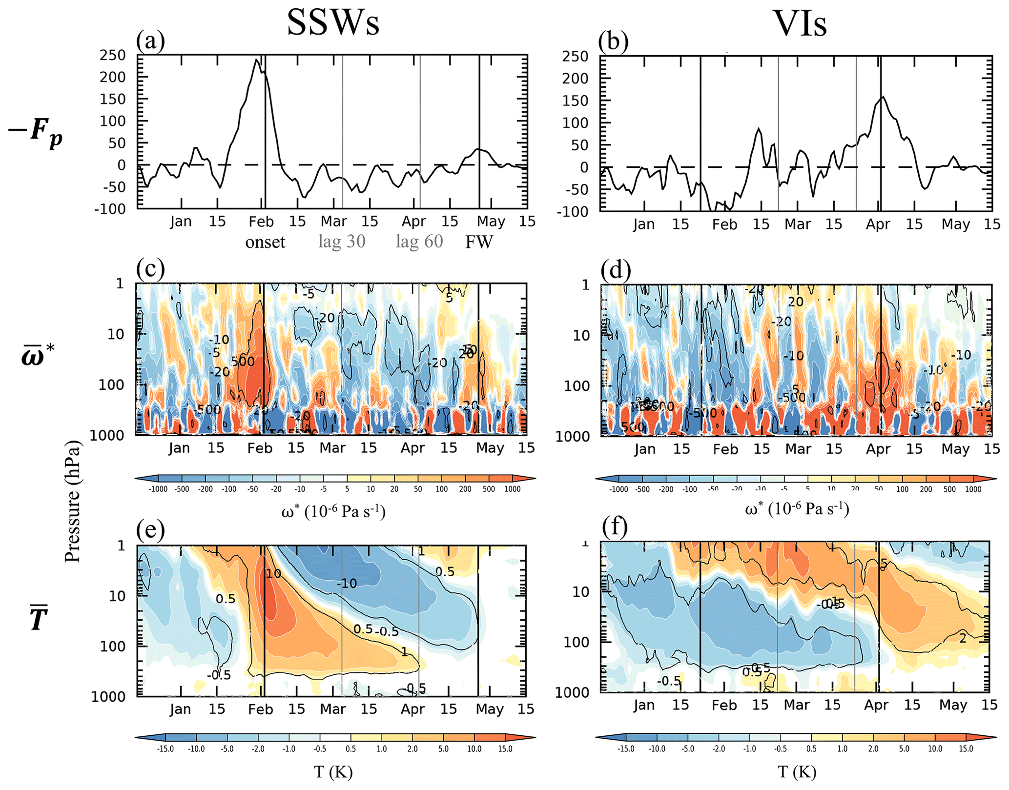
Figure 1SSW (a, c, e) and VI (b, d, f) composites over the Arctic. Shown are (a–b) the time series of 10 d smoothed vertical EP flux (10⁴ kg m s⁴) averaged over 40–80^∘ N at 100 hPa, and time–height cross sections for (c–d) the vertical component of the residual circulation (10⁻⁶ Pa s⁻¹; 65–85^∘ N) and (e–f) temperature (K; 65–90^∘ N). Contours represent the statistical significance at the 95 % level.

Download

SSWs (Fig. 1a, c, e) are typically preceded by enhanced stratospheric wave driving, starting at a negative lag of ∼ 15 d (Fig. 1a). This leads to the breakdown of the polar vortex and marks the onset of the SSW (Limpasuvan et al., 2004). After the onset, the wave driving decreases rapidly and becomes negative, contributing to the over-recovery of the vortex in the upper stratosphere, reminiscent of so-called polar-night jet events (de la Cámara et al., 2018a; Hitchcock and Shepherd, 2013; Kuroda and Kodera, 2001). As pointed out by Plumb and Eluszkiewicz (1999) and demonstrated by Fig. 1c, this cyclic nature of the wave driving imprints on the residual circulation of the entire stratosphere. Figure 1c shows that the vertical component of the residual circulation (${\stackrel{\mathrm{‾}}{\mathit{\omega }}}^{\ast }$) over the Arctic varies consistently with the wave driving, with enhanced downwelling during onset (reddish colors), followed by a long period of enhanced upwelling (bluish colors). The cycle ends at the end of winter, with somewhat enhanced wave driving and subsequent downwelling during the FW. Arctic temperatures (Fig. 1e) are characterized by cooling before the SSW, strong warming in the middle to lower stratosphere during and after the onset, and cooling after the onset in the upper to the middle stratosphere. The patterns of warming and cooling following the onset give the impression of a downward propagation. However, the cooling in the upper stratosphere is associated with the aforementioned suppressed wave driving and subsequent radiative cooling (Hitchcock and Shepherd, 2013; Limpasuvan et al., 2004), and the persistence of the warming in the lower stratosphere is related to the long radiative timescale in this part of the stratosphere.

VIs (Fig. 1b, d, f) are, in many respects, opposite to SSWs. As explained in Limpasuvan et al. (2005), VIs evolve relatively slowly and result from the sustained lack of stratospheric wave driving, leading to the gradual strengthening and cooling of the vortex. As shown by Fig. 1b, the wave driving is anomalously small, starting several weeks before onset and minimizing at about 1 week after onset. This is different from SSWs, as the wave driving during SSWs changes much more abruptly during onset. Long after the onset of VIs, the wave driving increases again, first more intermittently and then more systematically during the FW. We note that the magnitude of the wave driving associated with the FW is quite large and comparable to that of SSWs during onset. This may be attributable to the sustained suppression of wave driving during VI onset, contributing to the enhanced release of wave activity after the event and a relatively early FW. Also, the relatively strong polar vortex after VIs (not shown) is conducive to upward-propagating wave activity into the stratosphere.

As for SSWs, changes in the Arctic ${\stackrel{\mathrm{‾}}{\mathit{\omega }}}^{\ast }$ during VIs (Fig. 1d) agree well with the evolution of wave driving. The upwelling maximizes 1 week after VI onset, followed by a period of intermittent downwelling before the FW (see also Limpasuvan et al., 2005). VIs are also associated with pronounced and persistent Arctic cooling (Fig. 1f) in the lower stratosphere, which is in contrast to the significant warming that starts about 1 week before VI onset in the upper stratosphere. The warming slowly propagates downward, persists until spring, and finally becomes part of the FW that concludes the winter season. The timing and strength of the FW is another important difference between SSWs and VIs. While FWs after SSWs tend to be late and mostly represent a transition into climatology, FWs after VIs occur early, are relatively strong, and contribute to a pronounced weakening and warming of the vortex.

3.2 Arctic ozone changes

The above-described dynamical perturbations are associated with significant changes in the transport of stratospheric ozone and its temperature-dependent photochemical reaction rates. As has been shown to some extent before (Butler et al., 2017; de la Cámara et al., 2018b; Hocke et al., 2015), and as we will show in more detail next, this has major consequences for the distribution of stratospheric ozone.

We first examine the composite evolution of Arctic column ozone (i.e., the vertically integrated ozone amount) during SSWs (Fig. 2a). Red and gray shading indicate the deviation of the column ozone from its climatology (thick black curve), and the green line shows the percent column ozone anomaly with respect to climatology. Before onset, there is a subtle decrease in column ozone, presumably related to the anomalously strong and cold vortex during this time (Fig. 1e) and the reduced ozone transport into the polar regions. Within the first 10 d following the SSW onset, the column ozone anomalies rapidly increase by ∼ 50 DU and persist for up to 60 d until late winter. Hocke et al. (2015) suggested that the increases in column ozone after SSWs amount to up to 90 DU over the Arctic, which is nearly twice that of what we found. However, we note that the differences are only apparent as we show area-weighted latitudinal averages of column ozone and as the extreme ozone increases, in Hocke et al. (2015), occur only close to the pole. The vertically resolved Arctic ozone mixing ratio (Fig. 2c) shows a more complicated picture. There is a pronounced reduction in ozone in the middle and upper stratosphere after SSWs, which seems to be slowly descending downward. This decrease in midstratospheric ozone, which starts about 1 month after SSWs, has also been noted by Sagi et al. (2017). Ozone in the upper stratosphere also undergoes a complicated evolution. The negative anomalies above 5 hPa exist only shortly during the onset. They are followed by persistent positive anomalies, which again tend to descend downward by mid-March, diminish by April, and reemerge at midstratospheric levels by the end of April as a consequence of the FW.

Next, we examine the evolution of Arctic ozone during VIs (Fig. 2b, d, f). Column ozone (Fig. 2b) is anomalously negative over the entire VI life cycle, minimizing at about −40 DU by mid-March. Figure 2d demonstrates that the negative ozone anomalies maximize in the middle stratosphere at ∼ 10 d after onset and also tend to propagate downward into the lower stratosphere. These anomalies are particularly long lasting in the lower stratosphere, where they exist for more than 60 d until the FW. This composite behavior is very similar to the case study by Manney and Lawrence (2016), who reported that the rapid Arctic chemical ozone loss during winter 2015–2016 was abruptly terminated by the early FW in March. Ozone anomalies are also negative in the upper stratosphere, where they persist throughout the VI life cycle and tend to descend after the FW. At the FW, there are strongly positive ozone anomalies in the middle stratosphere. The structure of these anomalies is somewhat similar to that of SSWs, except that they are weakly negative in the lowermost stratosphere.

We now explore the role of the dynamical mechanisms that create the changes in ozone. From the TEM tracer transport equation Eq. (1), it is clear that several processes are involved. Figure 2e–j present the total time tendencies of ozone (Fig. 2e–f) and the contributions to it from vertical advection (Fig. 2g–h) and eddy flux convergence (Fig. 2i–j). The horizontal advection term is generally small and therefore omitted. For better orientation, the red and blue contours reproduce a constant ozone mixing ratio anomaly from Fig. 2c and d.

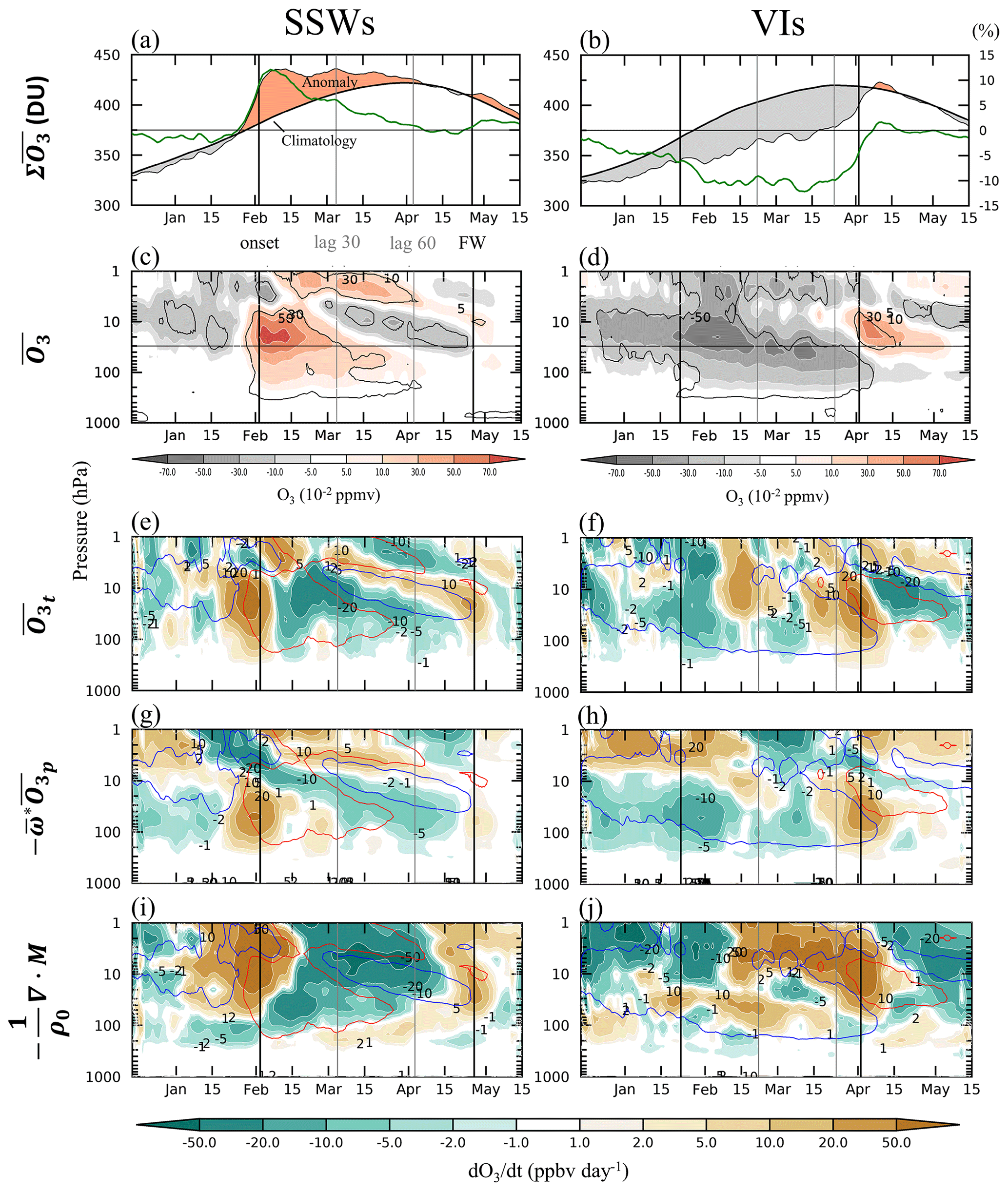
Figure 2Arctic ozone composites during (a, c, e, g, i) SSWs and (b, d, f, h, j) VIs. (a–b) Column ozone (left y axis) and associated percent anomalies with respect to climatology (right y axis); the horizontal line is the zero anomaly. The remaining panels are the anomalous time–height cross sections of (c–d) the ozone mixing ratio (10⁻² parts per million by volume – ppmv), (e–f) overall ozone tendency, ozone tendency due to (g–h) vertical advection and (i–j) eddy flux convergence (parts per billion by volume – ppbv d⁻¹). Quantities are averaged over 65–90^∘ N for ozone and 65–85^∘ N for tendencies. Horizontal lines in panels (c)–(d) mark the 30 hPa level, and the contours represent the statistical significance at the 95 % level. Contours in panels (e)–(j) represent the ±0.1 ppmv ozone anomalies from panels (c)–(d).

Download

The negative Arctic ozone anomalies in early winter, before SSWs, are partly the result of reduced eddy flux convergences (Fig. 2i) and vertical transport (Fig. 2g). The strong positive ozone tendencies close to the onset of SSWs, which are responsible for the increase in ozone after SSWs, result mainly from the convergence of eddy fluxes (Fig. 2i; see also de la Cámara et al., 2018b), triggered by the enhanced wave driving associated with SSWs (Fig. 1a). The downward transport of ozone by the enhanced residual circulation also contributes to the positive tendencies during onset, in particular in the lower stratosphere (Fig. 2g). After SSWs, the suppressed planetary wave activity leads to a sustained reduction in eddy transport and, hence, negative ozone tendencies in the middle and lower stratosphere. At the same time, the vertical advection of ozone is anomalously negative in the middle stratosphere after SSWs. Both effects lead to the gradual decay of the strongly positive ozone anomalies right after onset and eventually create the abovementioned banded structure of negative ozone in the middle stratosphere. Overall, this indicates that the decrease in midstratospheric ozone after SSWs is mainly of dynamical origin, consistent with de la Cámara et al. (2018b). We note that this does not support the ideas of Sagi et al. (2017), who argue that the ozone decrease is due to chemical reactions involving NO_x species. During the time of the FW, the eddy flux convergence becomes somewhat positive (Fig. 2i), leading, overall, to ozone mixing ratios that are close to climatology. In the upper stratosphere, the temperature-dependent photochemistry plays a dominant role for ozone. There, ozone is mostly anticorrelated with temperature (Craig and Ohring, 1958), which can be seen by comparing Fig. 1e (for temperature) with Fig. 2c (for ozone).

The VI-related total Arctic ozone tendencies (Fig. 2f) are mostly equal but opposite in sign to that of SSWs. VIs are passive events that develop gradually by radiative cooling out to space, and the related negative ozone anomalies appear long before the actual onset (Fig.  2d), which is related to periods of negative tendencies before and during VI onset (Fig. 2f). The tendencies are related to reduced eddy transport in the upper half (Fig. 2j) and reduced vertical advection in the lower half of the stratosphere (Fig. 2h). Ozone in the upper stratosphere slowly recovers towards climatology, mostly due to increases in eddy transport associated with pulses of planetary waves that restore the vortex back to normal. However, the positive eddy transport is counteracted by the photochemical effect as the temperature is anomalously warm in this layer (Fig. 1f). In contrast, the negative ozone anomalies in the lower stratosphere are sustained by reduced vertical advection (Fig. 2h) until mid-March. We also examined the source term S (not shown) and found negative tendencies in the lower stratosphere (10–100 hPa) during and after the onset of VIs, indicative of temperature-driven heterogeneous ozone depletion, as suggested by previous studies (Isaksen et al., 2012; Manney et al., 2011, 2020). In the upper stratosphere, S is, as expected, mostly anticorrelated with T. As explained before, FWs that follow VIs tend to be relatively strong and somewhat resemble SSWs, leading to sizable increases in Arctic ozone. As with SSWs, this is associated with positive eddy transport in the upper half (Fig. 2j) and positive vertical advection in the lower half of the stratosphere (Fig. 2h). The two effects compensate for the prior ozone deficits, leading to an overall recovery of the column ozone anomalies (Fig. 2b).

4.1 Tropical circulation changes

We now turn our attention to the tropics, defined as the ±15^∘ latitude band. Tropical ozone is changing in response to Arctic circulation events because of the global nature of the meridional overturning and its role in the transport of ozone (Randel, 1993). We start our discussion by focusing on the changing dynamics in the tropics during Arctic circulation events (Fig. 3). Note that no filtering has been applied to this figure, and that the shown changes can be due to both the remote impacts from the Arctic circulation events and the local effects from the internal variability associated with the QBO. However, the Arctic circulation events occur mostly at random, with respect to the QBO phase, so that the compositing largely removes possible QBO effects from the shown dynamical fields. This is also supported by the fact that Fig. 3 does not resemble the known influences of the QBO phases on the dynamics (e.g., Coy et al., 2016; their Fig. 8). During SSWs, the variations in ${\stackrel{\mathrm{‾}}{\mathit{\omega }}}^{\ast }$ (Fig. 3a) are largely opposite to those in the Arctic (Fig. 1c; de la Cámara et al., 2018a), except during the time of the FW. This demonstrates that the global nature of the enhanced residual circulation during SSWs also affects the tropics, leading to stronger upwelling and cooling. The cooling persists in the lower stratosphere, but quickly transitions into warming in the middle and upper stratosphere (Fig. 3c; see also Gómez-Escolar et al., 2014; Tao et al., 2015).

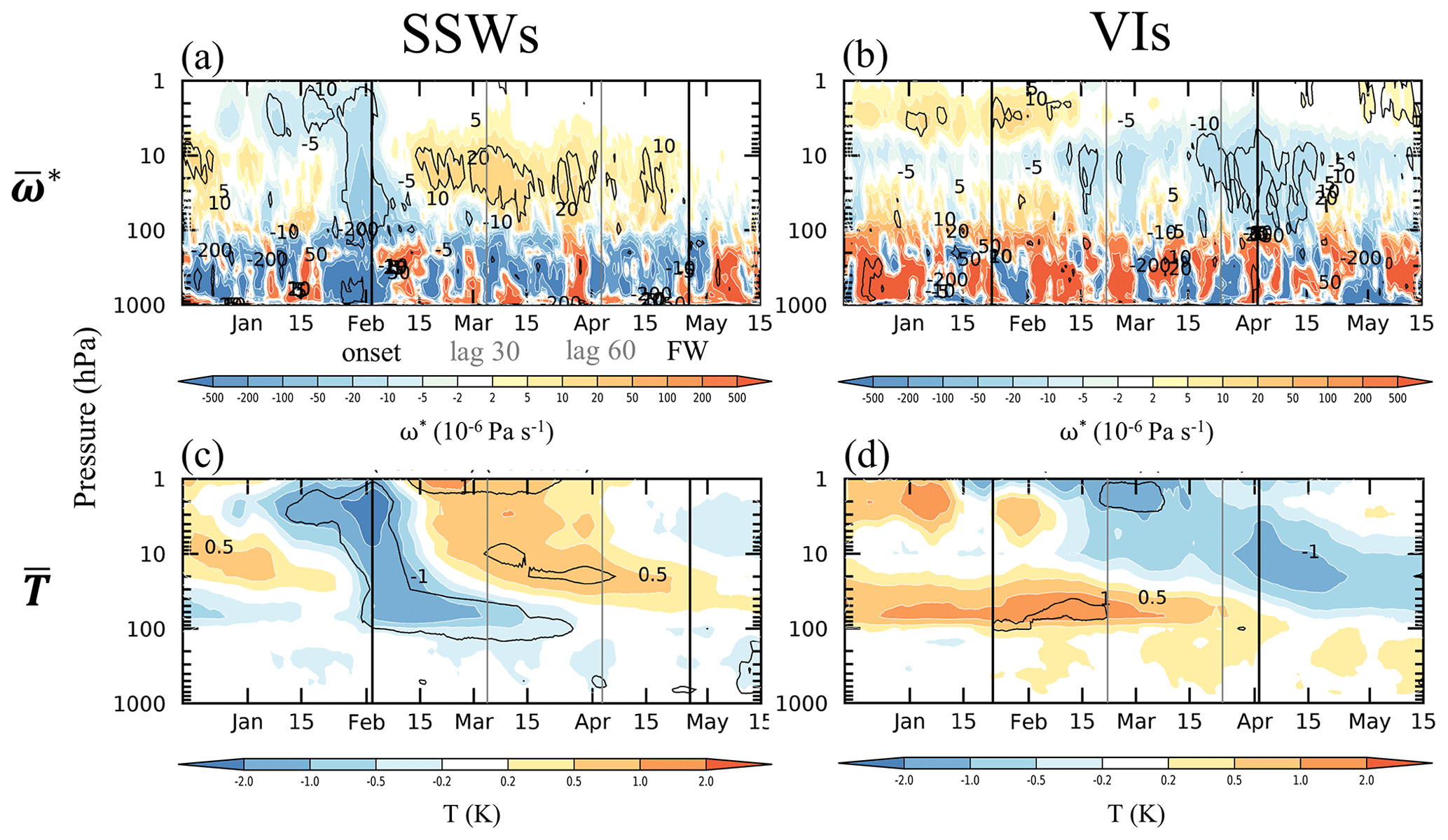
Figure 3Composite anomalies for (a, c) SSWs and (b, d) VIs over the tropical belt (±15^∘). Shown are time–height cross sections for (a–b) the vertical component of the residual mean circulation (10⁻⁶ Pa s⁻¹) and (c–d) temperature (K). Contours are as in Fig. 1.

Download

In comparison with the SSWs, the variations in ${\stackrel{\mathrm{‾}}{\mathit{\omega }}}^{\ast }$ during VI onset (Fig. 3b) are less well synchronized with those in the Arctic (Fig. 1d), perhaps due to the relative weakness of the wave driving and also due to influences from the QBO. Although ${\stackrel{\mathrm{‾}}{\mathit{\omega }}}^{\ast }$ is quite noisy, temperatures during VI onset show significant warming in the tropical lower stratosphere (Fig. 3d), which is probably related to adiabatic warming from anomalous downwelling (Fig. 3b). By mid-February, a downward-propagating cooling anomaly can be seen in the tropical upper stratosphere (Fig. 3d), as one would expect from the anomalous upwelling (Fig. 3b). As noted before, FWs after VIs are dynamically similar to SSWs, and this is also noticeable in the tropics. For example, the enhanced extratropical wave driving at the FW is also reflected in the tropical ${\stackrel{\mathrm{‾}}{\mathit{\omega }}}^{\ast }$.

4.2 QBO influences on tropical ozone

Understanding the changes in tropical ozone in response to Arctic stratospheric circulation events is complicated by the simultaneous influences from the QBO. To disentangle the two effects, we first examine how the vertical structure of tropical ozone changes in response to the QBO. Figure 4a shows the vertical cross section of tropical ozone anomalies (±15^∘) composited on the phase of the QBO from 16 QBO cycles. The black curve represents the mean evolution of UEQ30, where a QBO cycle is defined by two consecutive maxima in UEQ30. Assuming a mean QBO period of 28 months (Baldwin et al., 2001), a 1^∘ phase change of the QBO corresponds to ∼ 2.3 d. Tweedy et al. (2017) performed a similar analysis (their Fig. 1) by defining the central month of a QBO cycle from changes in the vertical wind shear at 40 hPa and taking QBO composites for different lags. Our results (Fig. 4a) are in good agreement with their study; for example, there is a nodal point of small ozone variations between 10 and 20 hPa, with much stronger variations above and below. Our result also agrees with Baldwin et al. (2001) that the maximum column ozone values occur when the westerly wind shear descends into the lowermost stratosphere. The vertical structure of the QBO ozone anomalies in Fig. 4a also shows two maxima at ∼ 10 and ∼ 30 hPa, shifted by about a quarter QBO cycle and consistent with previous findings (Coy et al., 2016; Randel and Wu, 1996).

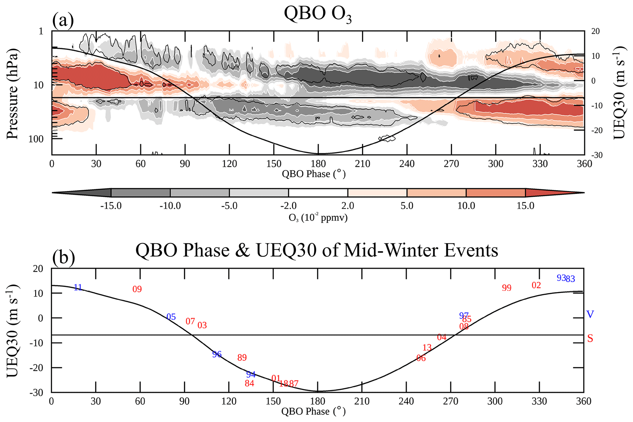
Figure 4Composites for QBO events. (a) QBO influences on tropical ozone – shading shows composite tropical ozone anomalies (±15^∘) from 16 QBO cycles (1980–2018), and black contours represent statistical significance at the 95 % level. A QBO cycle is defined by two consecutive positive UEQ30 maxima. (b) Central date timing of selected midwinter stratospheric circulation events relative to the QBO phase. Red (blue) numbers indicate years and QBO phase of SSWs (VIs); S and V on the y axis are the mean UEQ30 of all SSWs and all VIs (except 2016), respectively. The 2015–2016 QBO event has been purposely excluded from this analysis due to the anomalous nature of this event. The horizontal line is the climatological mean UEQ30.

Download

Figure 4b demonstrates that SSWs and VIs occur during virtually any phase of the QBO. However, as shown by the mean timing of the events (V and S markers on the right), there is a slight preference for SSWs to occur during the easterly QBO phase and VIs during the westerly QBO phase, a possibility that was discussed by Dunkerton et al. (1988). To filter out possible QBO influences from the tropical ozone, we define the QBO ozone signal as the mean ozone anomalies over days −60 to −30 with respect to the SSW/VI central date, which is then subtracted from the ozone associated with each Arctic circulation event. We used the resulting ozone anomalies to prepare Fig. 5c and d.

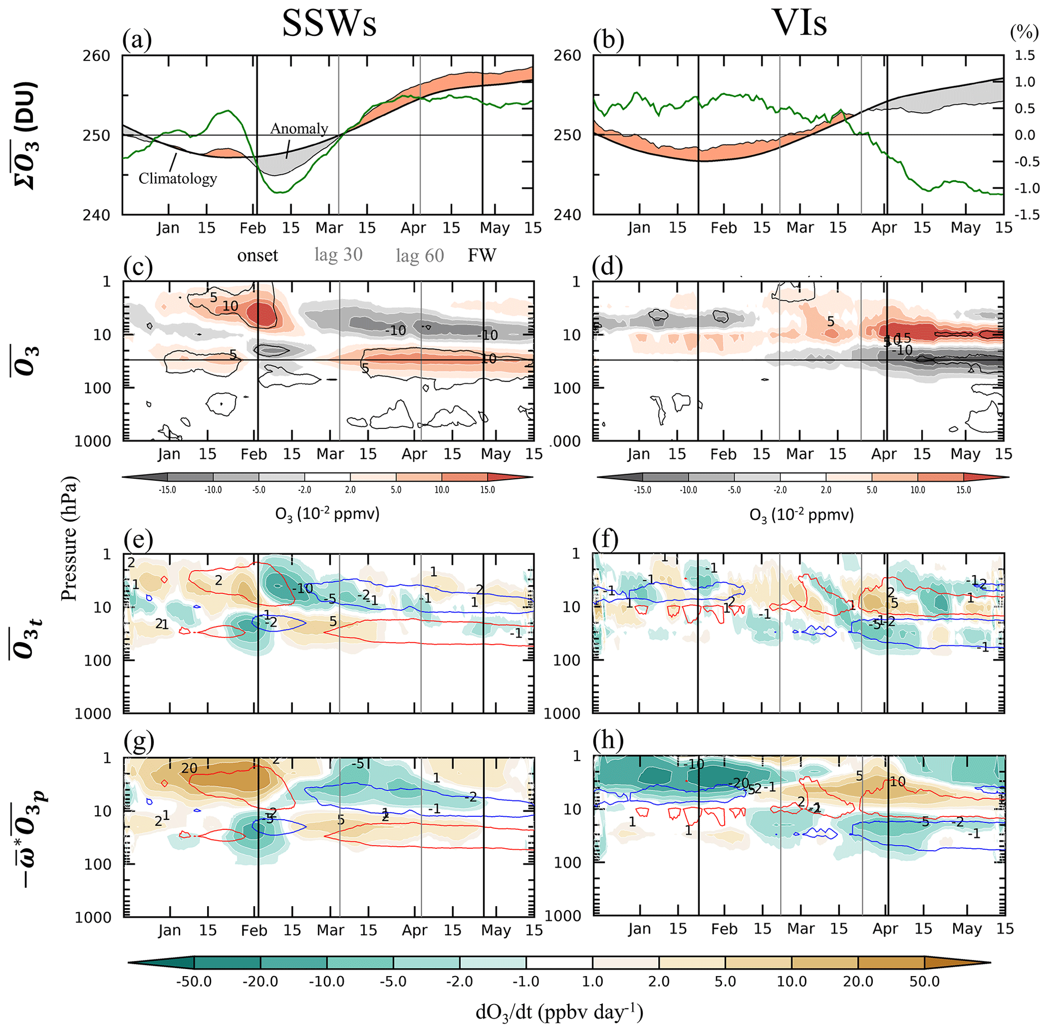
Figure 5As in Fig. 2, except for tropical ozone (±15^∘) and the exclusion of the eddy flux convergence term. Contours in panels (e)–(h) are the ±0.05 ppmv ozone anomalies from panels (c)–(d).

Download

4.3 Tropical ozone changes

Figure 5 presents composite anomalies and composite anomalous tendencies in tropical ozone during SSWs and VIs. The variations in tropical column ozone are rather small and amount to only ∼ 0.5 %–1 % of the climatological values, which can be compared to the 10 %–15 % changes seen over the Arctic. Nevertheless, the changes in tropical ozone are quite coherent and persistent. SSWs are followed by a small reduction in tropical column ozone by ∼ 2.5 DU (∼ −1 %) and an increase by ∼ 1–2 DU (∼ 0.5 %) after mid-March, which persists until late spring. Figure 5c shows the vertically resolved composite for tropical ozone after removing the preexisting ozone signal from the QBO, indicating that the local tropical ozone anomalies associated with SSWs are confined to levels above ∼ 60 hPa. During SSW onset, the response of ozone is characterized by significant increases in the upper stratosphere and decreases below the middle stratosphere (∼ 10 hPa), roughly opposite to those in the Arctic (Fig. 2c). The ozone anomalies reverse sign after mid-February and persist into late spring.

During VIs (Fig. 5b), there are small tropical column ozone anomalies, which are mostly positive (∼ 1 DU or 0.5 %) and only become negative (∼ 2 DU or 1 %) after the FW. However, the vertically resolved ozone anomalies with the QBO influence removed (Fig. 5d) show a weak dipole in the middle stratosphere around the onset, with little response in the lower stratosphere. This indicates that the increased column ozone anomalies in Fig. 5b are likely due to the QBO. As discussed before, the weak tropical ozone response to VIs is linked to the relative weakness of the wave driving during VIs, which is not sufficient to affect the tropical upwelling. However, during the FW of VIs, the wave driving anomaly is strong enough; the resulting tropical ozone response is similar to that during SSW onset, with a strong and persistent dipole centered at ∼ 20 hPa.

The dynamical mechanisms that create the changes in tropical ozone are dominated by vertical advection associated with changes to the residual circulation (Randel, 1993). Enhanced tropical upwelling during SSW onset (Fig. 3a) combined with a vertical background of ozone mixing ratios that maximize in the middle stratosphere create positive tendencies above 10 hPa and negative tendencies below 10 hPa (Fig. 5g). Following the reversal of the residual circulation anomalies at about 10 d after onset (Fig. 3a), the vertical advection term leads to oppositely signed ozone anomalies starting at about mid-February. During VIs, the tropical ozone tendencies (Fig. 5f) are mostly small. There are negative tendencies from vertical advection (Fig. 5h) in the upper stratosphere and during onset, owing to the weakened meridional circulation from the VI. However, these negative tendencies are compensated by the chemical source term (not shown), leading, overall, to little change in ozone. As expected, the tropical ozone tendencies during the FW of VIs (Fig. 5f) are mostly due to vertical advection (Fig. 5h) and compensating influences from the source term $\stackrel{\mathrm{‾}}{S}$ (not shown).