the Creative Commons Attribution 4.0 License.
the Creative Commons Attribution 4.0 License.
 | 20 Jul 2021
Experimental investigation of the stable water isotope distribution in an Alpine lake environment (L-WAIVE)
Patrick Chazette
Cyrille Flamant
Harald Sodemann
Julien Totems
Anne Monod
Elsa Dieudonné
Alexandre Baron
Andrew Seidl
Hans Christian Steen-Larsen
Pascal Doira
Amandine Durand
Sylvain Ravier
In order to gain understanding on the vertical structure of atmospheric water vapour above mountain lakes and to assess its link with the isotopic composition of the lake water and with small-scale dynamics (i.e. valley winds, thermal convection above complex terrain), the L-WAIVE (Lacustrine-Water vApor Isotope inVentory Experiment) field campaign was conducted in the Annecy valley in the French Alps during 10 d in June 2019. This field campaign was based on an original experimental synergy between a suite of ground-based, boat-borne, and two ultra-light aircraft (ULA) measuring platforms implemented to characterize the thermodynamic and isotopic composition above and in the lake. A cavity ring-down spectrometer and an in-cloud liquid water collector were deployed aboard one of the ULA to characterize the vertical distribution of the main stable water isotopes (HO, HO and H2H16O) both in the air and in shallow cumulus clouds. The temporal evolution of the meteorological structures of the low troposphere was derived from an airborne Rayleigh–Mie lidar (embarked on a second ULA), a ground-based Raman lidar, and a wind lidar. ULA flight patterns were repeated several times per day to capture the diurnal evolution as well as the variability associated with the different weather events encountered during the field campaign, which influenced the humidity field, cloud conditions, and slope wind regimes in the valley. In parallel, throughout the campaign, liquid water samples of rain, at the air–lake water interface, and at 2 m depth in the lake were taken. A significant variability of the isotopic composition was observed along time, depending on weather conditions, linked to the transition from the valley boundary layer towards the free troposphere, the valley wind intensity, and the vertical thermal stability. Thus, significant gradients of isotopic content have been revealed at the transition to the free troposphere, at altitudes between 2.5 and 3.5 km. The influence of the lake on the atmosphere isotopic composition is difficult to isolate from other contributions, especially in the presence of thermal instabilities and valley winds. Nevertheless, such an effect appears to be detectable in a layer of about 300 m thickness above the lake in light wind conditions. We also noted similar isotopic compositions in cloud drops and rainwater.


Why are the vertical structures of the stable isotope of the water vapour field in the lower troposphere only sparsely documented above Alpine lakes? This is in part due to the complexity and fast-evolving nature of the low-level atmospheric circulation in Alpine-type valleys which is intimately linked to the surrounding orography interacting with the synoptic-scale circulation. Thermally driven wind systems may be induced by hilly terrain, such as slope, mountain, and plateau winds (Kottmeier et al., 2008). Such winds result in mountain-venting phenomena that control the variability of the water vapour field in mountain catchment on very small timescales. Furthermore, small-scale inhomogeneity in soil properties across a mountain valley, as well as lake breezes resulting from land–lake temperature contrasts, may also induce the development of thermal circulations, particularly on clear-sky days, modifying the wind, humidity, and temperature fields on small spatial scales. The interaction of slope-driven and secondary circulations can furthermore influence the thermodynamical environment in the valley by the formation of convergence lines. Such convergence lines may favour the formation of shallow clouds and in some cases even deep convection (Barthlott et al., 2006). Interaction with the synoptic-scale circulation can lead to the formation of strong, gusty down-valley winds such as foehn events (Drobinski et al., 2007) and gap flows (Flamant et al., 2002; Mayr et al., 2007) that can also contribute to rapid modifications of the water vapour field in mountain catchment areas.
Stable water isotopes have long been used as a tool to study processes in lacustrine and hydrologic systems (see review by Gat, 2010), as well as evapotranspiration (e.g. Berkelhammer et al., 2016). For instance, an early study based on water stable isotope measurements conducted in the US Great Lakes region suggested that in the summer up to 15 % of the atmospheric water content in the atmosphere downwind of the lakes is derived from lake evaporation (Gat et al., 1994). Isotopic measurements of lake water have shown the relative roles of evaporation from the lake surface and transpiration from surrounding vegetation (Jasechko et al., 2013). The link between hydrology and evaporation has mainly been investigated using vapour and liquid water isotopes measurements gathered just above the Earth's surface and samples from lake water and precipitation (e.g. Cui et al., 2016).
Unexploited potential remains in using stable water isotopes to increase our understanding of the influence of evaporation, boundary-layer processes, and the free troposphere for local and regional climate conditions in Alpine lakes. For example, the depth of the atmospheric layer over which the influence of evaporation from the lake surface is detectable, and how different factors control the depth of this layer are still largely unknown. Detailed and comprehensive analysis of small-scale factors, such as winds in a valley, and how they are related to local and larger-scale dynamics, such as synoptic-scale subsidence in complex terrain, are therefore needed.
In order to get insights into such aspects, the L-WAIVE (Lacustrine-Water vApor Isotope inVentory Experiment) field campaign was conducted in the Annecy valley (45∘47′ N, 6∘12′ E; in Haute-Savoie in the French Alps) around the Lake Annecy between 12 and 23 June 2019. Being the second largest natural glacial lake in France, Lake Annecy is expected to play a substantial role for the regional hydrometeorology.
The overarching scientific objective of L-WAIVE field campaign is to study the vertical distribution of the water vapour contents and its heterogeneity over Lake Annecy. For this purpose, we have implemented an original multi-platform experimental approach based on continuous high-resolution vertical profiling of tropospheric water vapour, temperature, and wind, as well as scattering layers (aerosols, clouds) in the valley. Continuous atmospheric sampling was carried out by lidars together with airborne and boat-borne measurements of stable water isotopes (HO, H2HO and HO) in vapour, as well as liquid water sampling in the lake, clouds, and precipitation. A consolidated vision of water isotopes across the air–water compartments in the lake area is proposed. Special emphases are made on the interface between the lake and the atmosphere, as well as at the boundary with the free troposphere.
It is worth noting that we have defined such an observational strategy including ultra-light aircraft (ULA) means because measurements tall towers only provide incomplete information on the link between the different compartments in the free troposphere where the processes of mixing and distillation occur (e.g. Griffis et al., 2016; Steen-Larsen et al., 2013). In the past, He and Smith (1999) combined airborne measurements and surface sampling of the water isotope composition to study the evaporation process over the forests of New England, before the advent of high-resolution laser-based spectrometers. More recent available airborne measurements of the isotope composition in the boundary layer either focused on areas above the sea (Sodemann et al., 2017) or did not include measurements of the surface isotope composition (Salmon et al., 2019). The use of ULA makes it possible to sample the atmosphere very close to the surface up to altitudes of more than 4000 m and to fly in deep valleys (Chazette et al., 2005).
The rest of the article is divided into six sections. The experimental strategy is discussed in Sect. 2, whereas the instrumental platforms operations and environmental variables monitoring are presented in Sect. 3. In Sect. 4, we give the synoptic conditions of atmospheric circulation that help to understand the temporal evolution of the measurements in the valley, and more generally the meteorological conditions encountered during the field campaign. Atmospheric water vapour and liquid water isotopes, as well as lake water isotope observations made across the valley, are described in Sect. 5. In Sect. 6, the vertical distribution of water isotopes is discussed taking into account the vertical structures of the lower troposphere and the lake–atmosphere interface. We conclude in Sect. 7.
To achieve the scientific and methodological objectives of the L-WAIVE project, the field campaign was implemented in the southern part of Lake Annecy (the so-called “Petit Lac”), in the vicinity of the city of Lathuile (Fig. 1). Lake Annecy is bordered by the city of Annecy to the north, the Massif des Bauges to the west (2217 m above mean sea level – a.m.s.l.), the Massif des Bornes to the East (2438 m a.m.s.l.), and the depression de Faverges to the south (where Lathuile is located). Lathuile is located east of the foothill of the Roc des Boeufs (1774 m a.m.s.l.) to the west of the “Petit Lac” and the Tournette summit (2350 m a.m.s.l.) to the east. Lake Annecy, at a mean altitude of 446.7 m a.m.s.l., covers an area of roughly 27.5 km2 and has a mean (maximum) depth of 41.5 m (82 m).
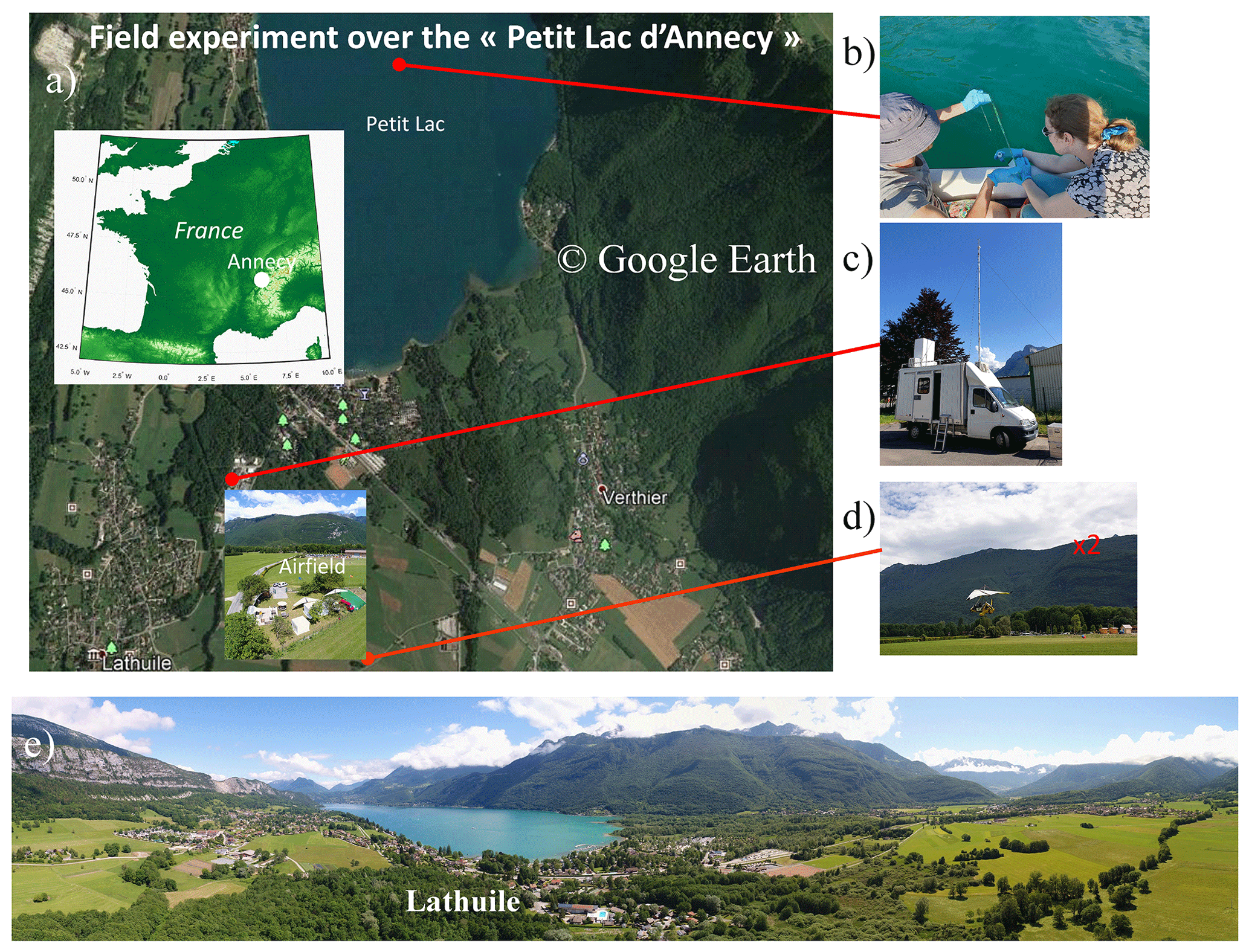
Figure 1Geographical location of L-WAIVE. The different pictures give a view of the environment where the measurements were performed and of the instrumented platforms used: (a) location of the experiment, (b) lake water sampling from a boat, (c) instrumented van, (d) instrumented ultra-light aircraft, and (e) panoramic view from UAV showing the location of Lathuile, as well as the Roc des Boeufs to the left, the Tournette summit to the right, and the “Petit Lac” in between.
2.1 Measurement platforms
Two airborne, one boat-borne, and one ground-based instrumented platforms were deployed in the vicinity of Lathuile in order to monitor humidity, temperature, wind, clouds, and aerosols in the lower troposphere over Lake Annecy and the surrounding valley environment, as well as to conduct measurements at the interface between the atmosphere and the lake, and in the lake. A brief overview of the platforms is given below, whereas the details on the instrumental payloads are given in Sect. 3:
- i.
Airborne platforms included the following:
- a.
One ultra-light aircraft (ULA) was mainly dedicated to remote sensing measurements. It allowed exploring the two- or three-dimensional structure of the lower troposphere thanks to a polarized Rayleigh–Mie lidar. It also carried a Global Positioning System (GPS) device and a meteorological probe (pressure, temperature, relative humidity). This will be referred to as “aerosol ULA” (ULA-A) in the following.
- b.
A second ULA carried both a cavity ring-down spectrometer (CRDS) water vapour isotope analyser, a meteorological probe for pressure, air temperature, GPS and relative humidity, and a cloud water collector. The platform offers the opportunity to measure the vertical profiles of temperature, relative humidity, H2HO, HO, and HO, and to collect cloud water samples. The latter were collected during specific cloud flights (when meteorological conditions were favourable) and the cloud collector was opened only in clouds. We will refer to this platform as “isotope and cloud ULA” (ULA-IC) in the following.
- a.
- ii.
For the ground-based platform, simultaneous high-resolution vertical profiles of water vapour, temperature, aerosols, and winds were acquired continuously from two co-located ground-based lidars.
- iii.
For the boat-borne platform, an instrumented boat allowed sampling the lake water by vials at the surface film and underneath (∼ 2 m deep) for the assessment of H2HO and HO. A CRDS water vapour isotope analyser performed measurements during 1 d at the end of the experiment just above the lake surface in parallel with the lake water sampling.
These different platforms are presented in Fig. 1 together with a view of the experiment site.
2.2 Deployment
Depending on the weather conditions, airborne platforms were deployed several times a day to document the temporal evolution of the atmospheric boundary layer over the lake. The days of operation of all platforms are summarized in Table A1 of Appendix A. The ground-based water vapour, temperature, and aerosol lidar operated continuously between 12 and 21 June in the morning (gathering over 220 h of data), while the ground-based wind lidar (WL) operated continuously between 14 and 23 June in the morning (acquiring also over 220 h of data). A total of 22 successful flights were conducted with ULA-A between 13 and 19 June, while ULA-IC performed 15 flights between 14 and 20 June. Valid cloud water samples were only obtained during the last three ULA-IC flights.
The CRDS previously installed on ULA-IC was mounted on the boat from 21 to 22 June. Boat-borne CRDS observations were made at the surface of the lake on the last outings of the boat. Nevertheless, lake water samples were taken on 14 occasions during the field campaign (see Appendix A). Finally, 28 samples of precipitation were taken during the campaign (7 of which were taken on 15 June in the afternoon) between 11 and 22 June 2019.

Figure 2Example of a typical ULA flight plan performed during L-WAIVE (performed on 17 June 2019). (a) The flight track adopted during the flight (blue dots for vertical profiling and red dots for horizontal exploration above the lake). DEM is the digital elevation model. (b) Schematic representation of the measurement strategy adopted during L-WAIVE. Two types of sampling strategy are illustrated: red for atmospheric sampling and green for cloud sampling. The purple arrows illustrate that the atmospheric sampling is performed during both ascent and descent.
On days when both ULA flew in coordinated patterns (13, 16–20 June), flights typically began with a profiling sequence between the surface and ∼ 4 km a.m.s.l., which was carried out in the vicinity of the two ground-based vertically pointing lidars (see Fig. 2). Soundings with levelled legs (see dotted blue line in Fig. 2a) were performed at a relatively slow ascent rate (∼ 60 m min−1) to ensure that the instruments were as close as possible to equilibrium with the environment. Upon reaching 4 km a.m.s.l., the flight route of the two ULA could differ, with ULA-A performing a high-altitude survey above Lake Annecy (see dotted red line in Fig. 2a), while ULA-IC was aiming for shallow cumulus clouds to sample cloud water droplets, as illustrated in Fig. 2b. Liquid water sampling was performed via multiple passes through the clouds to accumulate enough material to conduct isotope analysis. At the end of the flight, both ULA performed race-track descents around the ground-based lidars on their way back to the airfield.
During ascent and descent, the Airborne Lidar for Atmospheric Studies (ALiAS) aboard ULA-A was pointing sideways to directly derive the aerosol extinction coefficient (Chazette et al., 2007; Chazette and Totems, 2017). For the exploration of the valley at a cruising altitude between 3.5 and 4.5 km a.m.s.l., ALiAS was pointing to the nadir. The combination of both flight sequences thus allowed to survey the three-dimensional structure of the lower troposphere over the lake and its surroundings. The individual flight characteristics (time, maximum altitude, type of exploration) are presented in Appendix B for the two ULA (Tables B1 and B2 for ULA-A and ULA-IC, respectively).
This section provides a detailed description of the payloads on all platforms deployed during L-WAIVE. The periods of operation of each measurement platform are given in Appendix A.
3.1 Airborne payloads
We used two Tanarg 912 XS ULA from the company Air Création (Chazette and Totems, 2017). For each ULA (ULA-A and ULA-IC), the maximum total payload is of approximately 250 kg, including the pilot. Flight durations were between ∼ 1 and 2 h, depending on flight conditions, with a cruise speed around 85–100 km h−1. The ULA location was provided by a GPS and an Attitude and Heading Reference System, which are part of the MTi-G components sold by XSens.
3.1.1 ULA-A
Rayleigh–Mie lidar
ALiAS was especially developed by LSCE as an airborne payload dedicated to sample the atmospheric scattering layers and then the vertical structures of the atmosphere (Chazette et al., 2012, 2020). It emits a pulse energy of 30 mJ in the ultraviolet at 355 nm with a 20 Hz pulsed Nd:YAG laser (ULTRA) manufactured by QUANTEL™ (https://www.quantel-laser.com/, last access: 5 July 2021). The acquisition system is based on a PXI (PCI eXtensions for Instrumentation) technology. The receiver contains two channels for the detection of the elastic backscatter from the atmosphere in the parallel and perpendicular polarization planes relative to the linear polarization of the emitted radiation. The native resolution along the line of sight is 0.75 m, it is degraded here to 100 m during the data treatment to improve the signal-to-noise ratio. The wide field of view of ∼ 2.3 mrad ensures a full overlap of the transmit and receive paths close to 200–300 m from the emitter.
Meteorological probe
Part of ULA-A payload was a shielded meteorological probe VAISALA PTU-300 for measuring temperature, pressure, and relative humidity. This probe measures the atmospheric pressure, with a 1 min sampling time, within an uncertainty of 0.25 hPa, the air temperature within an uncertainty of 0.2 K and relative humidity (RH) within a relative uncertainty of 2.5 %.
3.1.2 ULA-IC
CRDS water vapour isotope analyser
ULA-IC carried a CRDS water vapour isotope analyser (L2130-i, Picarro Inc., Sunnyvale, USA; ser. no. HIDS2254) for the in situ measurement at about 5 Hz of the HO mixing ratio, and the isotope ratios δ18O and δ2H for HO and H2HO, respectively. Water vapour was drawn into the spectrometer through an unheated inlet of 68 cm length ( in O.D. stainless steel with SilcoNert coating), pointing backward on the left side of the aircraft at a distance of 38 cm from the CRDS. Pointing forward next to the vapour inlet, a fast-response temperature and humidity probe (iMet XQ-2, InterMet systems, USA; ser. no. 61124) measured thermodynamic properties (T, RH, p with uncertainties of 0.3 K, 5 %, and 1.5 hPa, respectively) and GPS location at 1 Hz. The CRDS analyser was operated in flight mode, with a flow of about 150 sccm through the inlet maintained by a membrane pump (part no. S2003, Picarro Inc.). Pressure and water vapour mixing ratio were corrected using calibration functions established at the FARLAB laboratory, University of Bergen, Norway. Raw measurements of the isotope parameters, expressed as δ values (see Appendix C), were corrected for the mixing ratio-isotope composition dependency and calibrated across the campaign period following recommendations from the International Atomic Energy Agency (IAEA; see Appendix D for details). Tests with a small bubbler system during the campaign indicated an anomaly in the CRDS measurements during 18–20 June, partially affecting two flights on the morning of 19 June and the first flight on 20 June. The anomaly was due to a saturated inlet system from condensate forming on the aircraft during a cloud sampling flight on 18 June. Flight periods affected by inlet saturation effects were excluded from further analysis (see Appendix D).
A time resolution better than 0.1 Hz was obtained for specific humidity from the CRDS and iMet probe, providing a spatial resolution of 200–300 m in the horizontal direction, and 10–50 m in the vertical, assuming a typical horizontal speed of 85–100 m s−1 and ascent rate of the aircraft of about 1–5 m s−1. Due to more complex memory effects, the isotope composition has lower effective time resolution (Sodemann et al., 2017; Steen-Larsen et al., 2014). We use here 10 s average data for all parameters on ULA-IC from upward profiles, filtered for rapid elevation changes, defined as exceeding 1.0 hPa ascent or 1.0 hPa descent within 10 s.
Cloud water collector
A pre-cleaned Caltech Active Strand Cloud Water Collector (CASCC, Demoz et al., 1996) was mounted on ULA-IC, modified to efficiently collect cloud water at the relative cruising speed of the ULA (85 to 100 km h−1). The CASCC was modified to efficiently collect cloud liquid droplets from the ULA. In order to sample droplets under the same conditions as those obtained on the ground, the CASCC fan was removed, and its inlet and outlet were prolonged with convergent and divergent high-density polyethylene (HDPE) cones to ensure an isokinetic air sampling. All parts necessary to adapt the HDPE cones on the CASCC were made of plastic. The flow through the probe must be steady and as turbulence-free as possible. The design of these modified inlet and outlet was calculated to get a constant mass of water droplets per time unit through the probe aboard the ULA. The resulting probe was installed on the side of the ULA, where the flow was assumed laminar and allowed air sampling with a flow rate of 35 to 47 m3 min−1, ahead of the motor exhaust. The CASCC strings and inlet were pre-cleaned with deionized water prior each flight and covered with a clean plastic bag when not in cloud (especially during take-off and landing). For a flight of 10 min inside a shallow cumulus cloud, the probe typically collected 41 to 48 g of cloud liquid droplets corresponding to a liquid water content of 0.10 to 0.16 g m−3, typical for such a cloud type (Herrmann, 2003).
3.2 Ground-based instrumentation
The ground-based scientific facility hosted by the technical department of the city of Lathuile was mainly composed of the Raman lidar WALI (Weather and Aerosol Lidar) and of a scanning Doppler lidar. WALI was embedded in the ground-based MAS (mobile atmospheric station; Raut and Chazette, 2009). The UAV (unmanned aerial vehicle) was also operated from this site, close to the lidar.
3.2.1 Raman lidar
WALI has been developed at LSCE (Chazette et al., 2014) based on the same technology as its precursor instruments LESAA (Lidar pour l'Etude et le Suivi de l'Aérosol Atmosphérique; Chazette et al., 2005) and LAUVA (Lidar Aérosol UltraViolet Aéroporté, Chazette et al., 2007; Lesouëf et al., 2013; Raut and Chazette, 2009). It is a custom-made instrument dedicated to atmospheric research activities.
The receiver of the lidar is composed of two distinct detection paths with a low full-overlap distance (∼ 150–200 m). The first path is dedicated to the detection of the elastic molecular, aerosols, and cloud backscatter from the atmosphere (Rayleigh–Mie lidar path). Two different channels are implemented on that path to detect (i) the total (co-polarized and cross polarized with respect to the laser emission) and (ii) the cross-polarized backscatter coefficients of the atmosphere. The second path, a fibered achromatic reflector, is dedicated to the measurements of the atmospheric Raman scattering, namely the vibrational signal for nitrogen (N2 channel) and water vapour (H2O channel) and the rotational signal to derive the temperature (T channel).
During the entire experiment, the acquisition was performed for mean profiles of 1000 laser shots, leading to a native temporal sampling close to 1 min. Rayleigh–Mie lidars are very efficient tools to detect scattering layers and then inform on the vertical structures of the atmosphere (e.g. Platt, 1977; Berthier et al., 2006; Chazette et al., 2020). The water vapour mixing ratio (WVMR) is retrieved with an absolute error less than 0.4 g kg−1 in the first 2 km above the ground level (a.g.l.) (Chazette et al., 2014; Totems et al., 2019). The calibration of the T channel is derived from the methodology presented by Behrendt (2006) and leads to an absolute error on the temperature lower than 1 ∘C within the first 2 km a.g.l. The final vertical resolution is set to 15 m below 1 km a.g.l. and 30 m above, and the temporal resolution is 0.5 h. In the following, a temporal resolution of 1 h is used.
3.2.2 Wind lidar
Wind profiles were measured using a scanning Doppler lidar (Leosphere Windcube WLS100). It operates in the infrared (1.543 µm) with a low pulse energy (0.25 mJ) but a high pulse repetition frequency (20 kHz). The Doppler shift due to the particles' motion along the beam direction (radial wind speed) is determined through heterodyne detection followed by fast Fourier transform analysis. The acquisition time was set to 1 s during the campaign. The pulse duration is 200 ns, corresponding to an axial resolution of 50 m given the pulse shape, with minimal and maximal ranges of 100 m and 7.2 km, respectively. The axial resolution can be lowered to 25 m by reducing the pulse duration (100 ns) while increasing the pulse repetition frequency (40 kHz), which in turn reduces the minimal and maximal range to 50 m and 3.3 km, respectively. In practice, the maximum range is limited by the signal level. A minimum carrier-to-noise ratio (i.e. signal-to-background-noise ratio) of −27 dB is required to keep the radial wind uncertainty (determined from the spectrum peak width) below 0.5 m s−1. Therefore, observations in the free troposphere are possible only when elevated layers of aerosols are present. Even in the boundary layer, several days of very low aerosol load occurred during the campaign, in which case the carrier-to-noise ratio threshold was lowered to −30 dB. With such a low carrier-to-noise ratio, the measurements must be considered with caution.
Profiles of the three components of the wind vector were determined using the Doppler beam-swinging technique originally proposed for Doppler radar (e.g. Koscielny et al., 1984). Here, the measurement cycle includes one vertical beam, for which the radial wind is the vertical component of the wind vector, and four slanted beams (15∘ from zenith) in the cardinal directions to derive the two horizontal components of the wind. The uncertainty on the horizontal/vertical wind components is determined using the variability inside averaging periods, possibly gathering several measurement cycles. During the campaign, the Doppler lidar was positioned in a wide valley (∼ 3 km at the observation site) with a rather flat bottom, and the closest distance existing between one of the slanted beams and an obstacle was ∼ 1 km. Therefore, the influence of the orography on the measurement is assumed to be negligible here.
3.3 Boat-borne payload: lake and atmospheric sampling
The lake water surface and subsurface were sampled at the middle of the “Petit Lac” to measure water isotopes and chemicals from the boat:
- i.
The lake water thermal stratification was monitored using an EXO sonde, equipped with temperature, pressure, pH, dissolved dioxygen, ion conductivity, and chlorophyll sensors. Profiles recorded in the middle of the “Petit Lac” (Fig. 1) once or twice per day (Table A1) and showed that the thermocline was typically at a depth of about 7 to 13 m, in good agreement with previous studies of the lake (Danis et al., 2003).
- ii.
Subsurface water samples were collected at a depth of 2 m in HDPE-capped flasks. Surface water samples were collected using a 30 × 30 cm silica glass plate immersed into water for a minute, then gently removed from water vertically (Cunliffe et al., 2013). The water falling from the plate in a continuous flow was not sampled; then, the dropwise water was collected in HDPE-capped flasks. The surface microlayer samples were then collected by scraping the remaining water on the glass plates (using a rubber scraper) in amber glassware capped vials. All liquid water samples were measured for isotopic composition (HO, H2H16O) at FARLAB, University of Bergen, according to established laboratory procedures (Appendix D).
- iii.
On 22 June, the CRDS isotope analyser was taken aboard the boat to sample a cross section in the atmospheric layer just above the “Petit Lac” through the location used for in situ sampling on the other days. This made it possible to capture the isotope concentrations as a function of the distance from the shore and the depth of the lake on that day. Water vapour isotope measurements were taken from an inlet at either ∼ 20 cm or ∼ 2 m above the water surface, while the iMet sonde measured temperature, relative humidity, and location. We used 2.5 m of in PTFE tubing and a 40 cm in stainless steel tip on the first inlet, and about 1.5 m of tubing with a 50 cm stainless steel tip. A flow rate of about 10 L min−1 was provided by an external manifold pump (N022AN, KNF, Germany) to either of the selected inlet lines. Post-processing and calibration of water vapour measurements were done as for the aircraft data (Sect. 3.1.2).
3.4 Precipitation sampling
Precipitation samples were taken throughout the campaign period. The sampling device consisted in a pre-cleaned HDPE funnel directly connected to a pre-cleaned HDPE sampling bottle. The precipitation samples were manually operated: after each precipitation event, the sample was aliquoted into 1.5 mL glass vials with rubber/PTFE septa and stored at 4 ∘C prior to isotopic analysis, while the rest of the sample was stored at −18 ∘C. Precipitation sampling times lasted from 20 min to several hours, depending on rainfall rate.
The synoptic and local weather conditions are analysed in the following, helping with the subsequent interpretation of the water vapour measurements in the lower troposphere over the Annecy valley.
4.1 Synoptic conditions
During L-WAIVE, France was under the influence of two main synoptic features, namely a pronounced trough over Brittany and the British Isles and a high-pressure ridge over northern Africa, sometimes extending across the Mediterranean and all the way into eastern Europe. This weather situation is illustrated in Fig. 3 using the fifth European Centre for Medium-Range Weather Forecasts Reanalysis (ERA5) at 0.75∘ horizontal resolution. This configuration caused a particularly strong pressure gradient over the western Mediterranean for the period 12–15 June (Fig. 3a), flanked in the east by an intense Libyan anticyclone, transporting warm air from subtropics to midlatitudes. The ridge weakened and broadened over the following days (16–19 June, Fig. 3b) before strengthening again (20–23 June) as the Libyan high intensified (Fig. 3c).

Figure 3ECMWF ERA5 temperature at 700 hPa (K, shading), geopotential height at 700 hPa (gpm/1000, contours), and horizontal winds at 700 hPa (black vectors) on (a) 14 June 2019 at 12:00 UTC, (b) 17 June 2019 at 12:00 UTC, and (c) 22 June 2019 at 12:00 UTC. The location of Lathuile is indicated with a grey dot surrounded by white.
During the course of the campaign, the area of interest was under the influence of warmer temperatures in the free troposphere linked with the high-pressure ridge at the beginning and the end of the field campaign, and colder temperature from 20 to 22 June. Since the experiment was conducted in a valley, where ERA5 reanalyses are generally considered not to be very accurate below the average altitude of the mountains (∼ 2 km a.m.s.l. in our case), it is more informative to use the measurements acquired during the field campaign from the lidar and ULA to describe the evolution of meteorological variables (wind, humidity, temperature, pressure).
4.2 Insight on the local atmospheric conditions derived from lidars
During L-WAIVE, the temporal evolution of the scattering layers, including clouds and aerosols, has been monitored using both the ground-based lidar (WALI) and the airborne lidar (ALiAS). They provide insight into air masses transport, weather situation, and local convection. For instance, such a capability was used to improve our understanding of atmospheric circulation in complex situations such as extreme heat wave phenomena (Chazette et al., 2017).
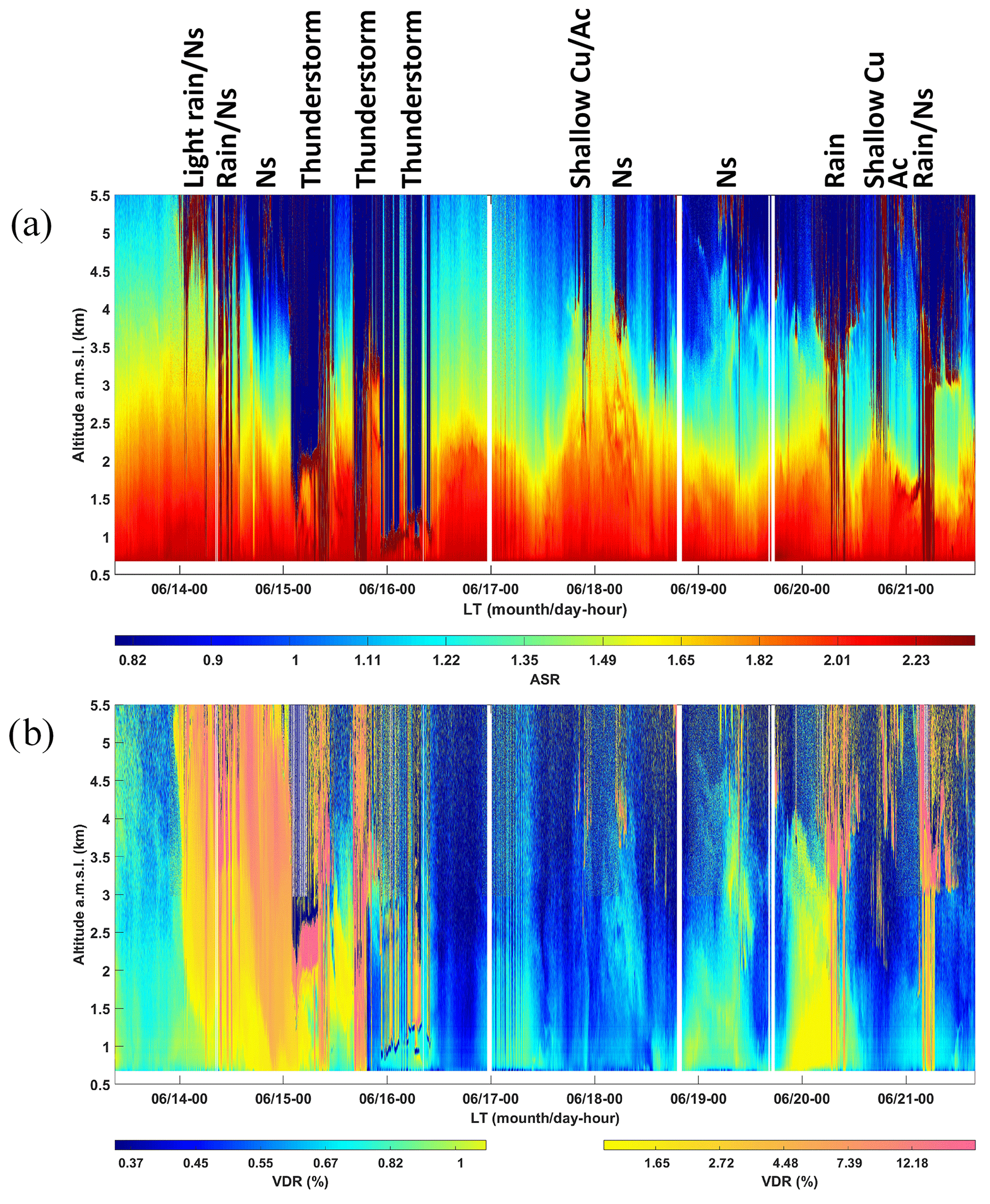
Figure 4Temporal evolution of (a) the aerosol scattering ratio (ASR) where the shaded areas correspond to the presence of clouds and (b) the linear volume depolarization ratio (VDR) from 13 to 21 June 2019. The cloud type and rain location are indicated, as is the type of the main aerosol structures identified by the VDR (orange/pink for dust on 14 June and other for pollution aerosols; clouds are in pink). Ns, Ac, and Cu indicate nimbostratus, altocumulus, and cumulus clouds, respectively.
Figure 4 shows the temporal evolution of the vertical profile of the aerosol (or cloud) apparent scattering ratio corrected from the molecular transmission (ASR, Fig. 4a) and of the linear volume depolarization ratio (VDR, Fig. 4b, Chazette et al., 2012). The vertical extension of aerosols in the valley is highly variable over time as is the presence and nature of clouds during the campaign. The strong diurnal cycle of ASR in the valley is tightly related to the slope winds and vertical stability associated with surface heating and the forcing due to the presence of clouds. The depth of the aerosol layer is the largest at the end of the afternoon when the convection is the strongest in the valley, while it is exhibiting a minimum around 11:00–12:00 LT when the valley winds reverse. The period was rather cloudy, with cloud types and the rainy periods including thunderstorms being indicated in Fig. 4a. In Fig. 4, we can clearly see the vertical updraft associated with clouds, which drives scatterers and water vapour towards higher altitudes, where there is a transition to the free troposphere. The transition is between the yellow and blue colours in Fig. 4a.
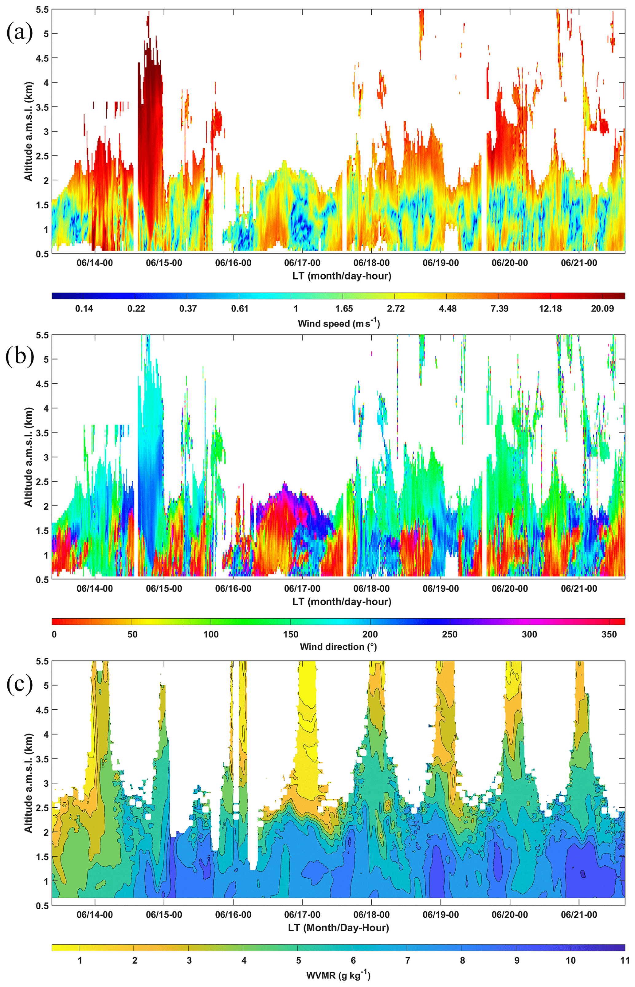
Figure 5Temporal evolution of (a) wind speed (m s−1), (b) wind direction (0∘ is for north and 90∘ for east) obtained from wind lidar, and the water vapour mixing ratio (WVMR) derived from the ground-based Raman lidar. White areas correspond to missing data caused by detection limitations of the lidar (signal-to-noise ratio, presence of clouds).
Significant day-to-day variations of the aerosol layer depth are thus observed during the field campaign which highlights local, regional, and synoptic-scale transport of air masses over the Annecy valley. At the beginning of the campaign (mainly on 14 June), large VDR values are detected up to altitudes exceeding 7 km a.m.s.l. (Fig. 4b). These large VDR values are related to a large-scale Saharan dust transport episode over the Lake Annecy valley favoured by the synoptic conditions on that day. These aerosols are progressively mixed downward by subsidence, reaching the valley floor around 00:00 LT on 15 June. The local wind in the valley is obviously disturbed during stormy periods and during the episode of long-range dust transport on 14 June. The presence of these aerosols at higher altitudes (up to ∼ 5 km a.m.s.l.) allowed the wind to be retrieved with the wind lidar above 2 km a.m.s.l. (Fig. 5a–b).
Strong southerly winds (in excess of 20 m s−1 above 3.5 km a.m.s.l.) were observed on 14 June in agreement with the synoptic meteorological fields. Weaker winds, less than 5 m s−1, are observed below 2 km a.m.s.l. for the entire period. The wind intensity does not show repetitive patterns from one day to the next. Nevertheless, it is rather in the course of the afternoon, when the wind comes from the north to the south, that we have the strongest velocities in the planetary boundary layer. Wind direction shows regular variations (Fig. 5b), with winds directed towards the south during the most of the afternoons. On the contrary, during the night and the first part of the morning, winds are directed towards the city of Annecy (north).
The vertical profiles of WVMR derived from the WALI ground-based lidar are also shown in Fig. 5c. They highlight highly variable water vapour in the first 2 km of the atmosphere, as is the case with wind. Generally higher WVMRs are often observed at night, associated with nighttime downslope winds, but may persist during days associated with heavy precipitation such as on 15 June 2019. The boundary between high and low humidity of the free troposphere is also highlighted, especially at night when the lidar exhibits enhanced sensing capabilities at higher altitude. For example, high humidity is seen up to ∼ 4 km a.m.s.l. on the night of 17–18 June in agreement with what is highlighted in Fig. 4a.
The wind at the surface of the lake controls evaporation and turbulent surface fluxes and influences the thermal convection, and cloud forcing influences the depth of the valley boundary layer, allowing the mixing of water vapour in a layer of variable thickness over time. The influence of the lake can therefore be seen up to altitudes of ∼ 4 km a.m.s.l., bearing in mind that the transition altitude to the free troposphere is generally of the order of 2.5 km a.m.s.l. here. The altitude of this sharp transition is also linked to the average altitude of the mountains surrounding the measurement site. There are no big differences between day and night on this boundary. It should be noted, however, that there are substructures that can be characterized by wind shears at different altitudes (Fig. 5b). A 0.5–1 km thick layer over the lake is thus highlighted, which can be linked to the wetter structures of Fig. 5c (in dark blue).
Water in vapour phase was sampled throughout the campaign in terms of mixing ratio of the main isotope and abundance of isotopes HO and H2H16O. At the same time, liquid water samples were taken from the surface of the lake, in the clouds, and surface precipitation to obtain their isotopic contents, and to place them in the context of the atmospheric water vapour of the lower troposphere. Water vapour was sampled in situ using a CRDS, whereas liquid samples, including precipitation, cloud water, and lake water, were analysed in the laboratory. Here, we report the isotope composition (see interpretative framework in Appendix C) as δ values relative to a standard (e.g. Gat, 1996).
5.1 Atmospheric in situ sampling
In total, 15 flights with ULA-IC have been performed (see Table B2), including 13 flights where the CRDS allowed a representative sampling of δ2H and δ18O (Appendix D). The isotope content δ2H observed during the flights ranged between about −340 ‰ and −80 ‰ for flight altitudes up to ∼ 3.5 km a.m.s.l., as shown in Fig. 6a. For this figure, we considered ascending and level flight segments, and excluded samplings with pressure increases larger than 1 hPa/10 s. As observed in earlier studies, the dataset is clustered along a typical mixing line in δ2H–q space (Noone, 2012; Salmon et al., 2019; Sodemann et al., 2017). The end members of the mixing lines show substantial day-to-day variations, from ‰ to −80 ‰ (∼ [−16, −12] ‰ for δ18O; not shown) for the more humid end member (q > 8 g kg−1) and from ‰ to −230 ‰ (∼ [−30, −20] ‰ for δ18O; not shown) for the drier end member (q < 3 g kg−1). It is important to keep in mind that both the variation in maximum flight altitudes and the meteorological situation can contribute to variability.
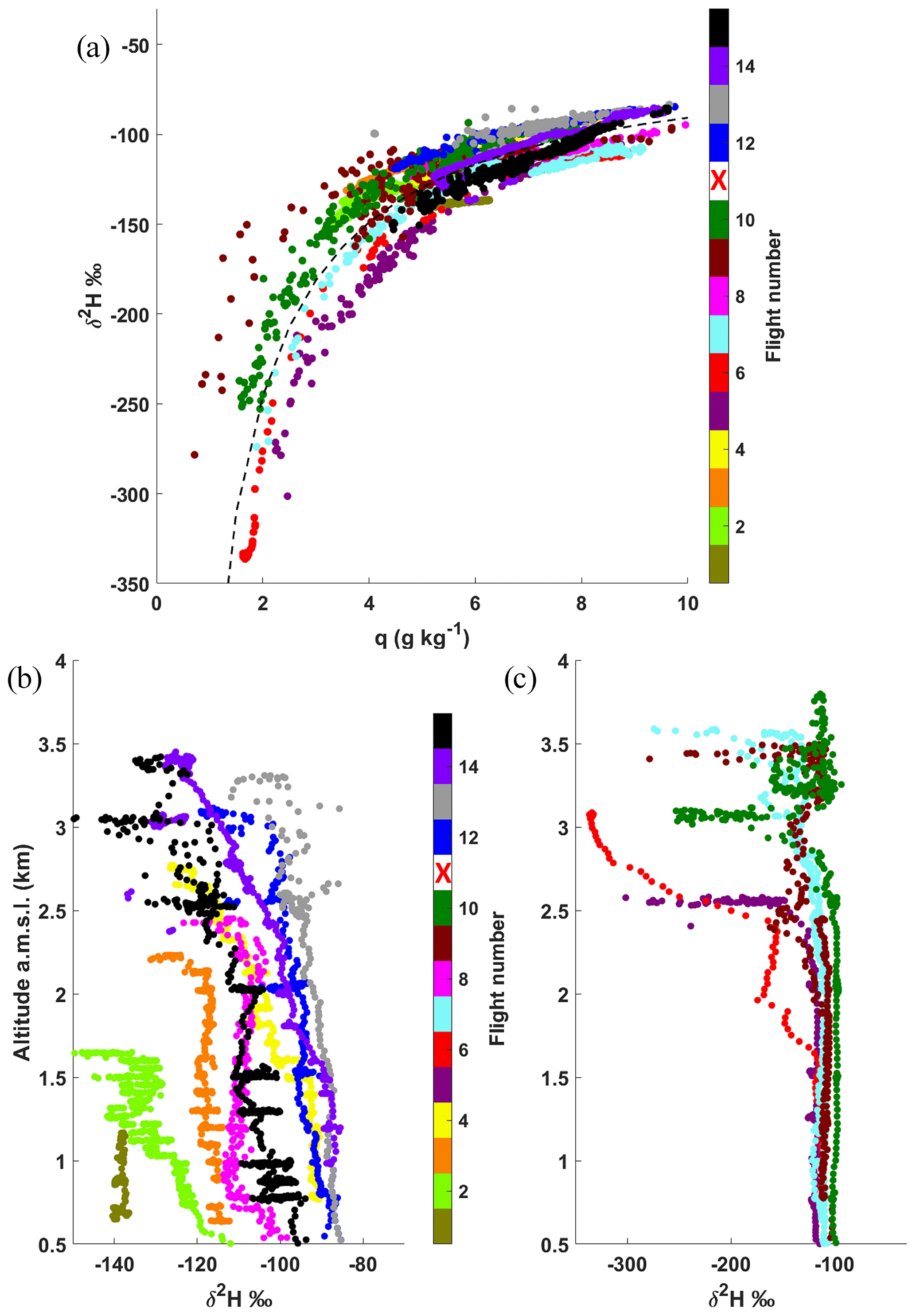
Figure 6Overview of airborne water vapour isotope measurements. (a) Isotope content δ2H (‰) vs. specific humidity (g kg−1). The mean mixing lines is computed following Noone (2012) with an end point q=1.37 g kg−1 and ‰, and reported using a dotted black line. (b, c) Vertical profiles of δ2H (‰). Colour indicates flight number. Panel (c) was added to separately plot the profiles with strong vertical gradients. Isotope data are averaged at 10 s intervals. The red cross associated with flight 11 indicates that no data were relevant during that flight.
As shown in Fig. 6b–c, the vertical profiles of the isotope content δ2H show small variability with altitude below 2 km a.m.s.l.; the greatest variability is observed in the first few hundred metres. In some cases, the profiles exhibit strong vertical gradients at higher elevations, as seen between 2.5 and 3.6 km a.m.s.l. during five flights (flights 5, 6, 7, 9, and 10). The same patterns are observed on the vertical profiles of δ18O (not shown) and even on the WVMR profiles derived from the meteorological probes aboard the two ULA. The sharp gradients are not observed systematically, as in the case of flight 15 (20 June), or may be present at a higher altitude, not sampled by the flight.
Indeed, because of the cloud cover and depending on the wind conditions, ULA have not been able to fly in the free troposphere on most days. However, this was possible for flight 10, where a marked reduction of δ2H occurred just above 3 km a.m.s.l., while higher values of isotopic content are seen at higher altitudes that match those below the transition. The same behaviour was observed on independent measurements of water vapour mixing ratio, which may suggest filamentation associated with differential transport of drier air layer in a wind shear zone. We will discuss this vertical distribution of isotopes in more detail in Sect. 5.2.5.
5.2 Cloud liquid water sampling
Four relevant cloud water samples have been taken with the CASCC on 18, 20, and 21 June (Table A1). The isotope content of the cloud liquid water is shown in Fig. 7a (coloured circles). It is close to the global meteoric water line (GMWL) with corresponding d-excess values ranging from 12.1 ‰ to 14.8 ‰. Equilibrium condensates were estimated from relevant water vapour isotope measurements during the time when the cloud samples were taken (Fig. 7a, coloured squares) using the fractionation factors of Majoube (1971), and air temperature measurements at cloud level, ranging between −4 and 1 ∘C. It is worth noting that given potential sources of uncertainty, the equilibrium condensate values agree remarkably well with the cloud liquid water during 18 June (green symbols) and the afternoon of 20 June (violet symbols). Overall, results here confirm that the cloud water droplets formed from equilibrium fractionation from ambient vapour. It is worth mentioning that such agreement between the completely independent sampling and measurement of vapour and cloud water supports the overall validity of (i) the cloud water sampling protocol, (ii) the airborne vapour isotope measurements, and (iii) the consistency of the calibrated water isotope dataset derived from the L-WAIVE campaign.
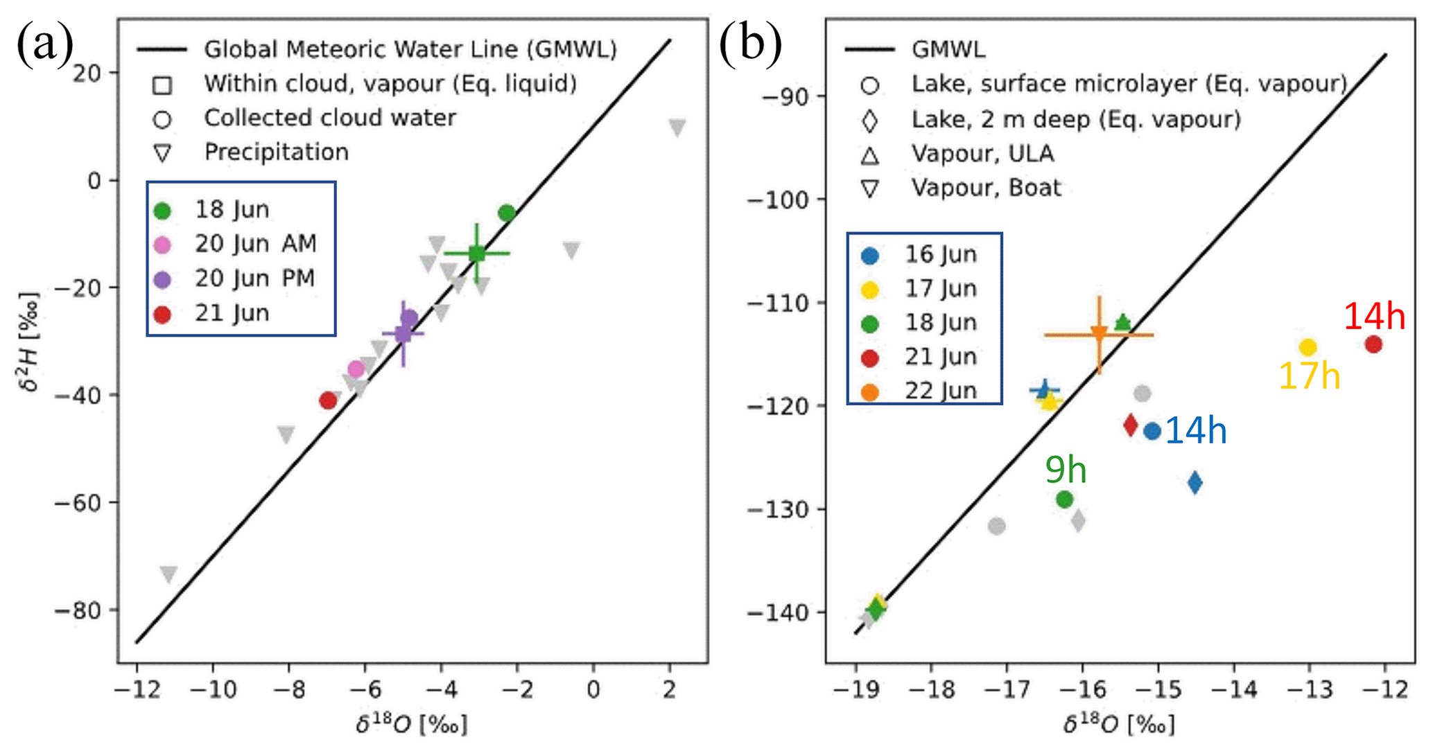
Figure 7δ2H−δ18O plots of liquid samples compared to the vapour isotope estimates. (a) Cloud water samples (circles), equilibrium condensate (squares), and precipitation samples (grey triangles). (b) Equilibrium vapour from lake water samples at various depths (dots and diamonds) compared to vapour isotope measurements from ULA-IC (upward triangle) and boat (downward triangle). Colour denotes matching dates (in the blue boxes are the colour legends in dot representation). Grey colours show data where the vapour samplings are not available. The times of the lake water sampling are indicated next to the dots with the same colours. The black line denotes the global meteoric water line (GMWL).
5.3 Precipitation liquid water isotope composition
In total, 28 precipitation samples, of which 22 are unique, have been taken during the campaign, with sampling times lasting from 20 min to several hours, depending on rainfall rate (Table A1). The isotope composition in rainfall ranges from −11.2 ‰ to 2.2 ‰ in δ18O and −73.5 ‰ to 9.6 ‰ in δ2H (Fig. 7a, grey triangles), with corresponding values of d excess between 3.5 ‰ and 20.8 ‰ (not shown). Even if evaporation effects from the sampling setup cannot be fully excluded, in particular for the samples with a sampling duration of more than 3 h, the consistency of duplicate samples indicate that the influence of sampling artefacts can overall be considered as limited. Notably, there is an overall correspondence between the isotope range observed in cloud water samples and in a majority of precipitation samples. Deviations of precipitation samples from the GMWL indicate potential below-cloud exchange processes between the falling raindrops and the ambient water vapour, leading to an enrichment of the precipitation in 18O (Graf et al., 2019; Worden et al., 2007). We have noticed that samples taken between 12 to 15 June, and on 21 June are most enriched in 18O, exhibiting the higher values in δ18O and δ2H and a smaller d excess. These samples are from rainfall events associated with local thunderstorms. The corresponding low d excess (even negative, ∼ −8 ‰) of these samples may point to the partial evaporation of rain droplets during their fall.
5.4 Lake liquid water isotope composition
Evaporation from Lake Annecy is expected to be an important source for the water vapour in the low troposphere above the Annecy valley. In order to link the atmospheric profiles of water vapour isotopes to the lake as a moisture source, 20 lake water samples (Table A1) were taken throughout the campaign within the lake–atmosphere interface layer (6 samples), as well as close to 2 m depth (14 samples), and analysed for their stable water isotope composition. The average isotope contents were found to be −8.3 ± 1.5 ‰ for δ18O and −63.0 ± 6.0 ‰ for δ2H. To assess the isotopic balance between the lake water and the water vapour isotope composition measured by ULA and boat, we calculated the equilibrium vapour for the lake surface temperatures measured during respective days (Fig. 7b) using the equilibrium fractionation factors of Majoube (1971).
Lake water samples taken close to the surface are expected to be most affected by evaporation, causing deviations to the right from the GMWL along evaporation lines (enrichment in 18O) and corresponding to a negative d excess. As a matter of fact, lake water samples clearly cluster on the right-hand side of the GMWL (Fig. 7b, diamonds), whereas vapour data from the ULA-IC (triangles) and the boat (downward triangle) are to the left, with a relatively consistent range of isotope values. The corresponding d excess underline this result for the six lake water samples from the lake–atmosphere interface layer, with values of the d excess ranging between 2.2 ‰ and −19.6 ‰ and an average value of −6.3 ‰. For the samples taken at a depth of 2 m (Fig. 7b, diamond symbols), the derived d excess showed less evaporation influence, with a mean of 0.6 ‰ and a standard deviation of 8.2 ‰. While some sampling artefacts cannot be fully excluded, the fact that there are differences between the isotope contents at the lake surface and 2 m depth points to the impact of ongoing evaporation that decreases with depth. We note that temperature profiles taken within the lake show a typically strong thermocline below about 7 m depth during summer (Danis et al., 2003). Therefore, freshwater input from runoff and precipitation, and loss to evaporation are expected to primarily affect the warmer, upper mixed layer within the timeframe of the campaign.
The range of equilibrium vapour for δ2H observed in lake water for 16 and 17 June (Fig. 7b, blue and yellow dots) matches to first order with the range of δ2H from ULA-IC. However, the δ18O in equilibrium vapour is substantially higher than the measured vapour value. This pleads for a kinetic (non-equilibrium) fractionation during lake evaporation. During 18 June (Fig. 7b, green dot), equilibrium vapour of the liquid samples has a lower heavy isotope content than observed by ULA-IC, pointing to the influence of other factors on either atmospheric or lake water composition on these days. However, one should be rather cautious about this interpretation, as the time of the lake water sampling (∼ 09:00 LT) was significantly different from the time of the flight (flight 9 of ULA-IC, ∼ 12:00 LT), while for 16 and 17 June, the measurements were performed at the same time. It is worth noting that Lake Annecy is fed by a catchment whose surface is 10 times larger than that of the lake via 10 main tributaries located on the lake periphery. The flows of its tributaries increase significantly in situations of heavy rain, which can substantially influence the isotopic content of the lake during the course of a year; however, on 17 and 18 June, no rain was observed.
During the two main sunny days of the field campaign (17 and 18 June), the evolution of isotope content profiles in the low troposphere (up to 3.5 km a.m.s.l.) is analysed together with the other observations including lidar measurements. In a second step, we provide a statistical overview of all the available data to compare the various samples from the lake water to the low troposphere, including clouds, and precipitation.
6.1 Vertical profiles in the low troposphere as observed from ULA
Figure 8 shows the vertical profiles corresponding to four coordinated flights between the two ULA. These flights were carried out in the late morning and afternoon during the two sunny days of the campaign, i.e. 17 and 18 June. The profiles were constructed by averaging the data over 100 m bins. This operation makes it possible to improve the signal-to-noise ratio and to evaluate the dispersion of the measurements as a function of altitude (coloured areas in the figure).

Figure 8Vertical profiles of the isotope composition δ2H from CRDS (ULA-IC), specific humidity (from WALI and meteorological probes aboard ULA), potential temperature (from meteorological probe of ULA-A), wind speed components from the wind lidar, and apparent scattering ratio (ASR) derived from the airborne lidar ALiAS (ULA-A) on (a) 17 June in the morning (∼ 10:30–12:00 LT), (b) 17 June in the afternoon (∼ 16:00–18:30 LT), (c) 18 June in the morning (∼ 11:00–12:30 LT), and 18 June in the afternoon (∼ 16:00–18:00 LT). The dispersion on the data is represented by the coloured areas.
The vertical structures of the lower troposphere are well reproduced across all data types, showing the consistency of the isotopic profiles with the independent observations. The strong gradients on δ2H above 2.5 km a.m.s.l. are related to the transition to the free troposphere and are confirmed by the lidar observations and meteorological measurements on the two ULA. Discrepancies appear between the specific humidity measured from the two ULA on 18 June above 2.7 km a.m.s.l. (Fig. 8c). This can be explained by the presence of a fractional cloud cover. The ULA-IC has crossed part of the cloud base which is at the interface with the free troposphere.
In the morning, the atmosphere near the lake shows near-surface stability over 200 to 300 m which deteriorates/mixes away in the afternoon according to the potential temperature profiles. A few hundred metres above the lake, the atmosphere is very stable on 17 June in the morning (Fig. 8a); it then loses stability in the afternoon due to thermal convection (Fig. 8b). On the morning of 18 June, the stability is strong below 1.5 km a.m.s.l. (Fig. 8c) and approaches the neutrality above this altitude. In contrast to 17 June, an atmosphere close to neutrality is observed in the afternoon on 18 June (Fig. 8d), which may favour vertical exchanges from the lake surface to the free troposphere. An important difference between the 2 d is also related to the surface wind speed. Winds of the order of 5 m s−1 were present on 17 June, whereas they were close to null on 18 June. Therefore, significant differences in water exchange between the lake and the atmosphere can be expected between the 2 d. These differences have already been noted when comparing the samples in Fig. 7b. On 17 June, wind-forced evaporation phenomena may therefore intervene which may explain at least part of the assumed isotopic fractionation. On the other hand, on 18 June, we have seen that the water samples are hardly representative for ULA measurements as they were taken early in the morning, before the sun lit up the valley. Around noon, the structure of about 300 m observed at the bottom of the δ2H profile (Fig. 8d) and found in the other data is certainly strongly influenced by evaporation from the lake. It is significantly attenuated in the afternoon due to vertical mixing linked to thermal convection. We observe an enrichment in 2H in this layer compared to the rest of the vertical profile in the morning that may be due to the lake evaporation into depleted air.
6.2 Statistical overview of isotopic content from the lake to the atmosphere
The main atmospheric vertical structures are derived from the profiles of potential temperature, aerosols, wind, and water vapour mixing ratio. We have therefore defined three layers in the low troposphere: (i) between the lake surface to 1 km a.m.s.l., (ii) between 1 and 2.5 km a.m.s.l., and (iii) between 2.5 and 3.5 km a.m.s.l. The uppermost value represents our altitude sampling limit. The first layer can be identified as the lake boundary layer, the second layer is associated with the region of influence of the lake, below the altitude of the surrounding mountains, and the third layer is the transition towards the free troposphere influenced by the regional circulation. The location in altitude of these different layers obviously depends on the weather conditions and the time of day.

Figure 9Whisker boxes for (a) d excess, (b) δ2H, and (c) δ18O. For each subfigure, the upper part depicted the statistical content of isotope in water vapour and the bottom part in the liquid water. For each whisker box, the central continuous vertical line indicates the median (50th percentile, P50), and the bottom and top edges of the box indicate the 25th (P25) and 75th (P75) percentiles, respectively. The whiskers extend to the most extreme data points not considered outliers, which are values outside the interval bounded by the 5th and 95th percentiles. For the atmospheric water vapour, the number of samples n is indicated close to the boxes. The confidence interval at 95 % defined by is represented by the notches in the upper part of the subfigure.
Using the vertical layering introduced above, the overall results for stable isotopes in water are summarized in Fig. 9 on a statistical basis selecting the highest-quality data. This synthesis is presented in the form of whisker boxes for d excess (Fig. 9a), δ2H (Fig. 9b), and δ18O (Fig. 9c). For each subfigure, the upper part depicted the statistical content of isotope in water vapour for each sampled altitude range in the atmosphere, while the lower part describes the same thing for liquid water samples collected from clouds, precipitation, and in the lake, at the interface and subsurface. For the atmospheric water vapour, the sample number n is significant (numbers given at the right of the whisker boxes in Fig. 9b), and it makes sense to accurately assess the confidence intervals at 95 %. As the notches do not overlap from an atmospheric layer to another, we can conclude, with 95 % confidence, that the true medians do differ. Hence, we highlight a significant variability in the stable isotope content of water vapour depending on the atmospheric layers previously identified.
Between the surface of the lake and 2.5 km a.m.s.l., we find δ18O values are in the lower range to those recorded by Craig and Gordon (1965) for evaporation over the Mediterranean [−15, −10] ‰. On the other hand, they report much more dispersed d-excess values ranging from 5 ‰ to 35 ‰. Gat (2000) gives narrower values for marine and European air masses with a d-excess interval of [7–11] ‰. Our observations are mainly outside this interval for the first two layers; they overlap it for the 2.5–3.5 km a.m.s.l. layer more influenced by the synoptic scale. Measurements from the boat on the last day of the campaign within 1 m above the lake are overall consistent with the vapour isotope measurements made by ULA-IC on previous days in the lake boundary layer.
Based only on the statistical information content provided by the whisker boxes profiles, it is difficult to see precisely whether the evaporation of lake water significantly influences the first layers of atmosphere just above the lake. Indeed, different factors can influence the relation between water vapour measured by the ULA above the lake and the evaporating water vapour. In addition to the immediate evaporate, water vapour can be advected and mixed in from other locations horizontally but also vertically. In particular for a lake with coastal, vegetated areas within less than about 2 km distance anywhere on the lake, influences from evapotranspiration are likely within the lower 1 km above the lake.
Our liquid water samples are not numerous enough to define a confidence interval. As explained previously, we nevertheless note an enrichment in heavy isotope of the surface layer of the lake which is directly in contact with the atmosphere and therefore directly subject to evaporation. The 2 m depth layer is significantly less enriched as evidenced by their isotope content. We highlight therefore a significant enrichment in heavy isotopes of surface water associated with low values of d excess, which is characteristic of evaporation as described by Gibson and Edwards (2002). Measurements of δ18O profiles in Lake Annecy have already been carried out between the years 2000 and 2002. They have shown δ18O values of the order of −9.5 ‰ for water above the thermocline of the “Petit Lac” during the summer months (Danis, 2009), in agreement with our results. This indicates a year-to-year stability of the isotopic content of the lake water below the surface microlayer.
From a first analysis of our successful airborne in situ sampling of water vapour isotopes and cloud water, we conclude that cloud water formed in an equilibrium fractionation process for the samples collected here, and the cloud water isotopes were relatively similar to local precipitation (taken on other days). Since 1992, the Global Network of Isotopes in Precipitation (GNIP, https://nucleus.iaea.org/wiser, last access: 5 July 2021) regularly samples rainwater at Thonon-les-Bains (60 km northeast from Annecy) for isotope analyses. Based on data available until 2018, typical summer δ18O (δ2H) values fall within the interval [−16, −1] ‰ ([−120, −20] ‰), encompassing our precipitation and cloud water measurements. It should be noted that the lake water is poorer in heavy isotopes than rain and cloud water. This difference is probably due to snowmelt during spring and the contribution of precipitation falling at high altitude. Note that GNIP data show median values of −10.5 ‰ (−78.6 ‰) for δ18O (δ2H) during winter versus −6.5 ‰ (−43.5 ‰) during summer which agree with the studies of Dutton et al. (2005) and Kendall and Coplen (2001).
The L-WAIVE field campaign documented for the first-time vertical profiles of stable water isotopes over an Alpine lake valley, in combination with lidar and meteorological measurements. Within L-WAIVE, we have developed an innovative approach to retrieve the vertical profiles and their heterogeneity over Lake Annecy in several meteorological situations. The field campaign took place between 12 and 23 June 2019 and used the complementary and/or synergistic measurements from different means of sampling gaseous and liquid water, atmospheric scattering layers, and meteorological parameters (temperature, moisture, and wind). Continuous high-vertical-resolution profiles of tropospheric water vapour, temperature, and wind, as well as aerosols in the Annecy valley have been performed using ground-based lidars. They were acquired together with boat-borne and airborne measurements of stable water isotopes (H2O, H2HO, and HO) in the lake, in the lower atmosphere as well as in precipitation and in-cloud using an original sampling method from ULA. The atmospheric structure over Lake Annecy has been simultaneously measured using an nadir-looking airborne lidar coupled with a meteorological probe on a second ULA.
Strong temporal variability of several measured parameters has been observed during the field campaign, with a marked diurnal cycle influenced by the valley winds and the vertical thermal stability. The valley winds particularly influence the water vapour composition of the atmospheric layers near the lake, over a thickness of about 300 m. Thermal instabilities which evolve strongly during the day, and which can be associated with cloud forcing at the base of the free troposphere (between 2.5 and 3.5 km a.m.s.l.), will rapidly mix water vapour throughout the air column between the lake and the base of the free troposphere. This process makes it difficult to observe the influence of evaporation from the surface waters of the lake. We also note strong vertical gradients in the abundance of isotopes at elevations higher than 2.5 km a.m.s.l., with a marked decrease at the interface with the free troposphere. Such vertical structures are confirmed by the other types of measurements, including lidar profiles of aerosol backscatter. The altitude at which these gradients were observed exhibited a day-to-day variation throughout the measurement campaign in relationship with stratification in the valley, weather conditions, and topography.
We note that the cloud water samples are close to the GMWL (d excess between 12.1 ‰ and 14.8 ‰), which indicates that the cloud water formed from equilibrium fractionation of ambient atmospheric water vapour. There is an overall correspondence between the isotope range observed in cloud water samples and a majority of precipitation samples (d excess between −8.6 ‰ and 20.8 ‰ for the minimal and maximal values, and of ∼ 7 ‰–13.5 ‰ between the 25th and 75th percentiles). The deviations observed on precipitation samples that are below the GMWL indicate potential below-cloud exchange, or post-condensational exchange processes. It is also worth noting that the average isotope composition of the lake water, taken at 2 m depth, appears different from the one for the surface microlayer sample; this may be due to evaporation processes. The δ18O in equilibrium condensate above the lake is generally substantially more depleted, confirming the existence of non-equilibrium fractionation that could be due to both lake evaporation and air mass advection.
During the two sunny days of 17 and 18 June, it was noted that the effect of the lake on the water vapour content of the valley is difficult to isolate because it involves different processes, including the variability of thermal convection and horizontal advection processes associated with valley winds. Nevertheless, this effect appears to be detectable on a layer of about 300 m thickness above the lake in light wind conditions. The field experiment that was carried out is complex; however it would need to be repeated several times in order to have representative statistics on favourable cases such as the one on 18 June, i.e. with negligible surface winds.
Table A1Data available during the period of the field experiment between 11 and 23 June 2020. The cross (“X”) indicates that the ULA or instrument was operated on a half-day basis. The malfunctions are denoted by “M”. The number of flights is indicated per ULM for each half day. For in situ samplings, the number of samples per half day is indicated. During the first two flights of the ULA-IC, the iMet sonde was not operating (denoted by italic numbers). A sequence of ULA-IC flights experienced saturation in the inlet, which requires data filtering (denoted by bold–italic numbers).
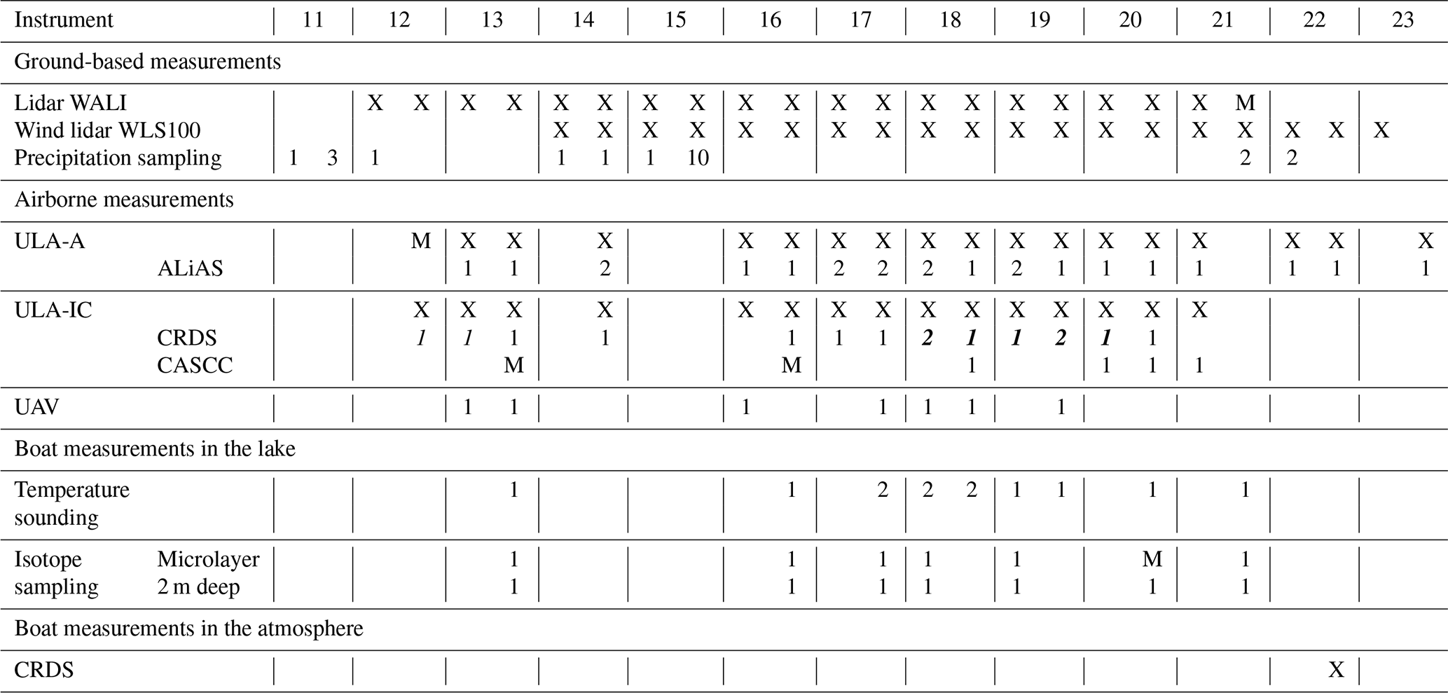
Table B1Flights characteristics for the remote sensing payload (ULA-A).
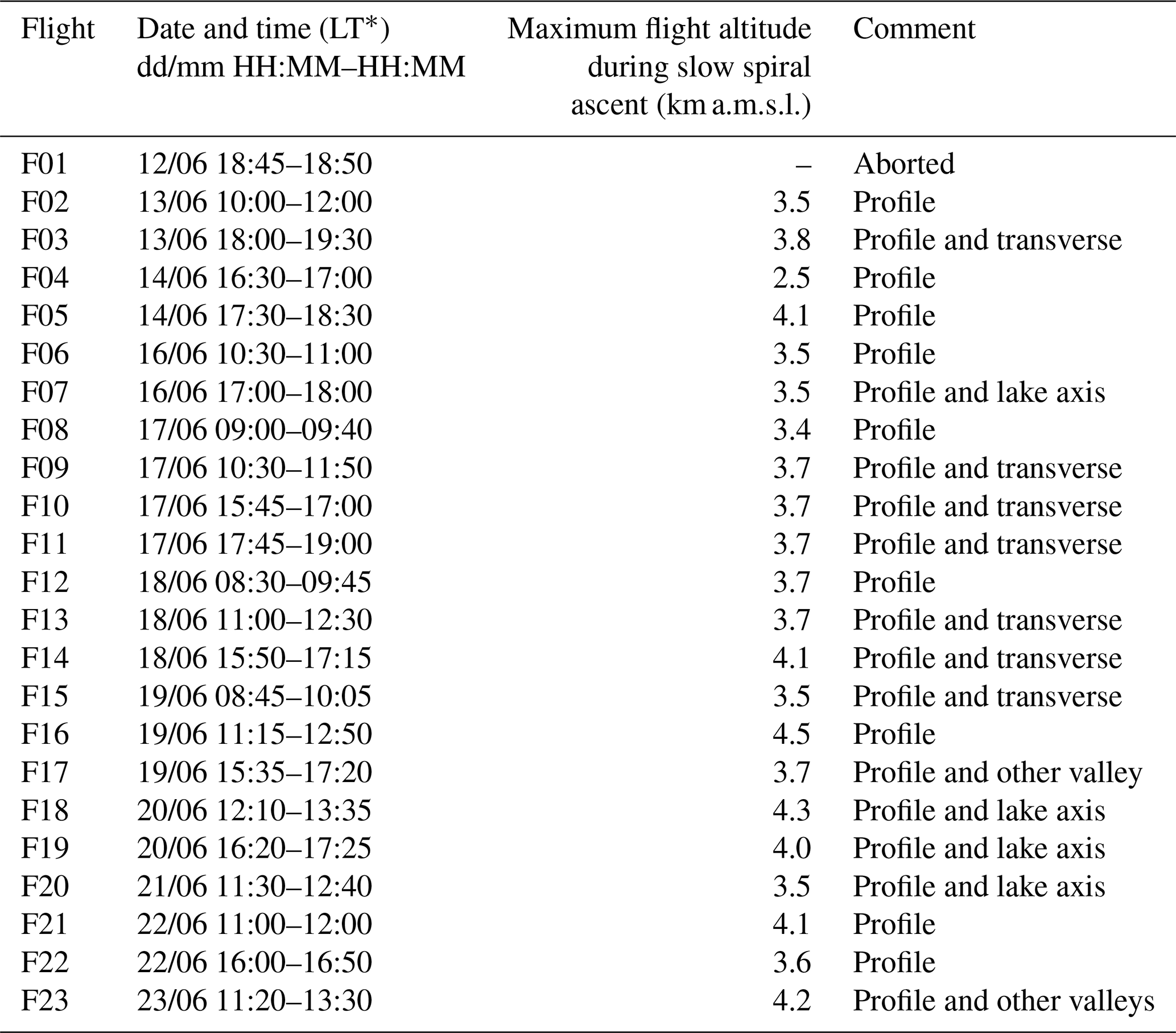
∗ Local time (LT).
Table B2Flights characteristics for the in situ payload (ULA-IC).
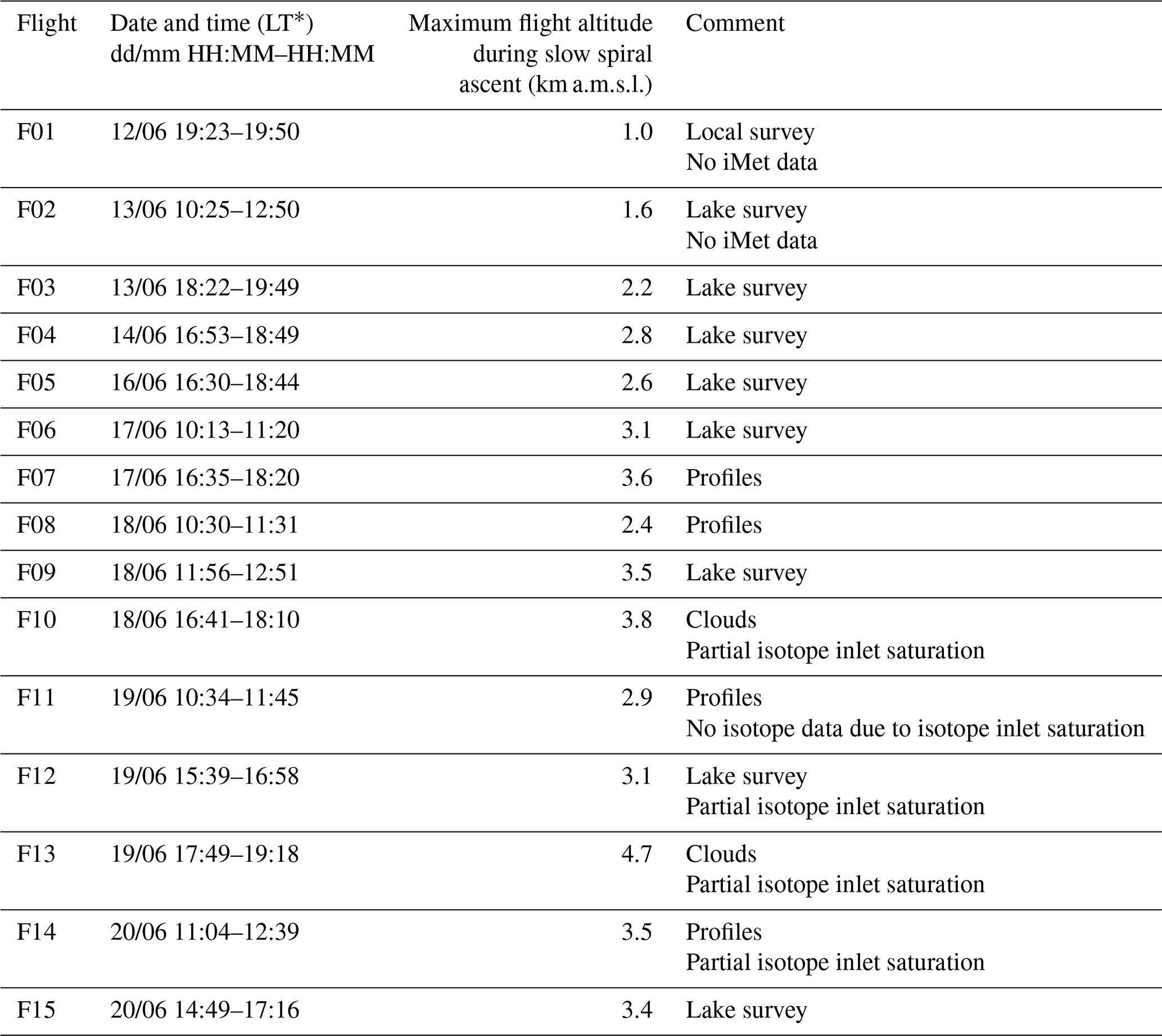
∗ Local time (LT).
The isotope composition δ2H and δ18O are given by the relationships
where is the isotope ratio of Vienna Standard Mean Ocean Water (VSMOW) for the compound X and RX the isotopic ratio given by
The d excess (d) is therefore defined as
to measure the deviation from equilibrium fractionation, noting the global average value for precipitation d=10 ‰ (Dansgaard, 1964).
D1 Processing of liquid samples for stable water isotope analysis
Liquid water samples were processed at FARLAB, University of Bergen, according to established laboratory routines. For isotopic analysis, liquid water samples were transferred to 1.5 mL glass vials with rubber/PTFE septa (part no. 548-0907, VWR, USA). An autosampler (A0325, Picarro Inc.) injected approximately 2 µL per injection into a high-precision vaporizer (A0211, Picarro Inc., USA) heated to 110 ∘C. After blending with dry N2 (< 5 ppm H2O) the gas mixture was directed into the measurement cavity of a cavity ring-down spectrometer (L2140-i, Picarro Inc., Sunnyvale, USA) for about 7 min with a typical water concentration of 20 000 ppm. Three secondary laboratory standards were measured at the beginning and end of each batch for calibration purposes. Batches consisted typically of 20 samples, with laboratory drift standard DI, measured every five samples. For calibration according to International Atomic Energy Agency recommendations (IAEA, 2009), 16 injections of the laboratory standards EVAP (δ2H=4.75 ± 0.11 ‰, δ18O=5.03 ± 0.02 ‰) and GSM1 were used and averaged over the beginning and end of each batch for calibration. Typical short-term reproducibility is 0.3 ‰ for δ2H and 0.04 ‰ for δ18O. Long-term measurement accuracy is better than 0.66 ‰ for δ2H, 0.15 ‰ for δ18O, and 0.83 ‰ for the d excess, evaluated from the 1σ standard deviation of the analysis of an internal laboratory standard over 1 year.
D2 Processing of stable isotope measurements in water vapour
Raw measurements of pressure and water vapour mixing ratio of the CRDS (Picarro L2130-i, ser. no. HIDS2254) were corrected using calibration functions established at the FARLAB laboratory, University of Bergen, Norway. Raw measurements of the isotope parameters, expressed as δ values relative to VSMOW2 (Vienna Standard Mean Ocean Water 2), were corrected for the mixing ratio-isotope composition dependency using time-constant correction functions obtained for this analyser according to the method of Weng et al. (2020). For calibration (Fig. D1), vapour isotope data were transferred onto the VSMOW2-SLAP2 scale by routine measurements of secondary laboratory standards using a Picarro Standard Delivery Module (SDM, part no. A0101, Picarro Inc.) before and after the campaign. Hereby, secondary laboratory standards GSM1 ( ± 0.30 ‰, ± 0.05 ‰), and DI ( ± 0.37 ‰, ± 0.07 ‰) were measured repeatedly for 20 min in the period 1 June 2019 to 19 July 2019. Calibrations of the CRDS analyser in the laboratory before and after the field deployment showed minor drift during the measurement period (GSM1 δ18O: 0.002 ‰ per month, DI δ18O: −0.233 ‰ per month, GSM1 δ2H: 1.045 ‰ per month, DI δ2H: −0.853 ‰ per month). From 2σ standard deviations of all valid SDM calibrations, the combined calibration uncertainty is estimated to be on the order of 0.2 ‰ for δ18O and 2 ‰ for δ2H. A small bubbler system was used in the field for testing instrument drift before and after flight operations in the field. These tests indicated an anomaly in the CRDS measurements 18–20 June, partially affecting two flights in the morning of 19 June and the first flight on 20 June. The anomaly was due to a saturated inlet system from condensate forming on the aircraft during a cloud sampling flight on 18 June. Flight periods affected by the saturated inlet were excluded from further analysis, as well as the entire flight 11 of ULA-IC, and are indicated with a corresponding quality flag in the data files (Table B2).
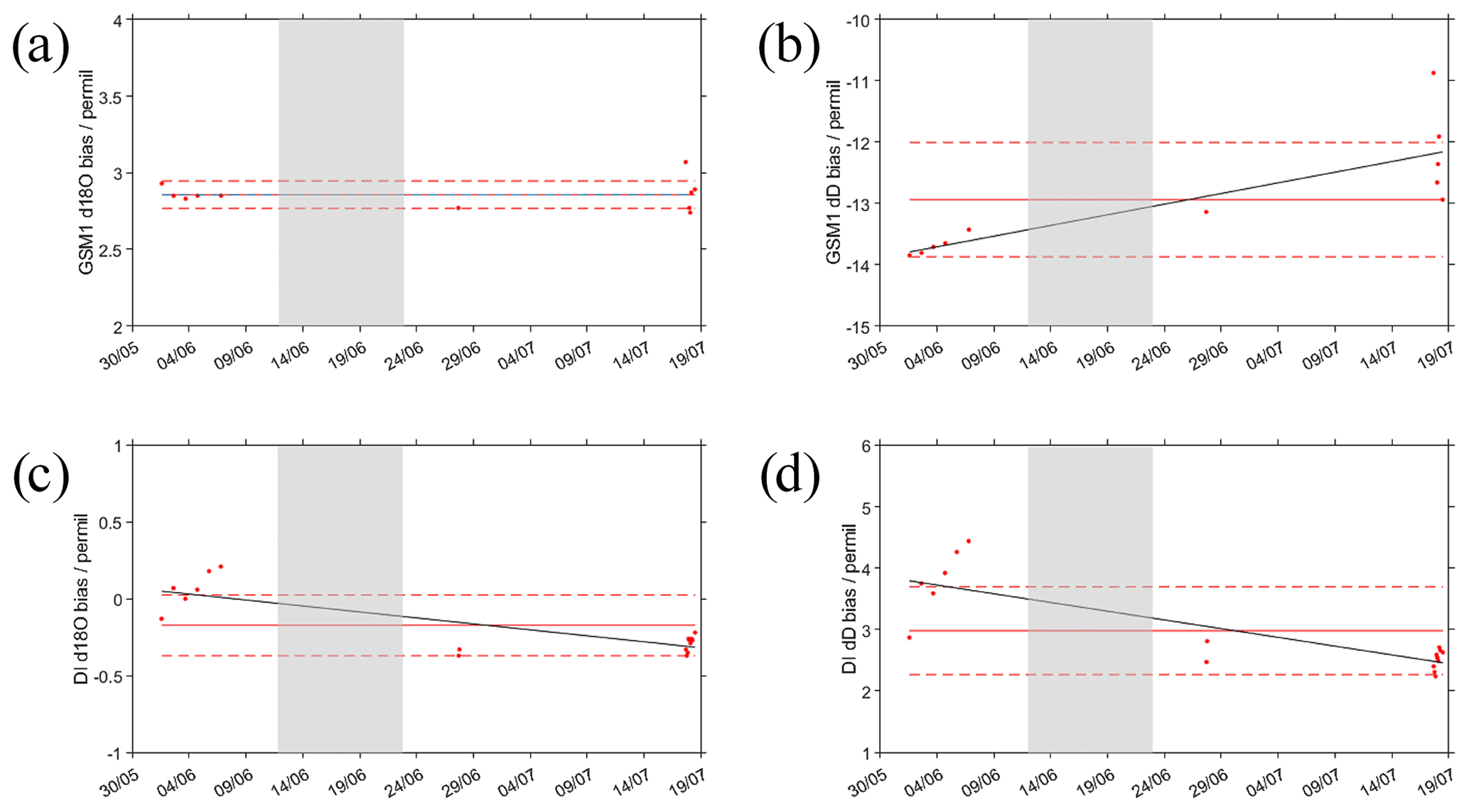
Figure D1Bias between nominal and raw delta values obtained with the SDM with working standards DI and GSM1 on analyser HIDS2254 before and after the L-WAIVE campaign period. Grey area denotes campaign period. Red lines denote the mean and 1σ standard deviation of all valid SDM calibrations in the period 1 May to 19 July 2019. The black line is a linear regression line.
D3 Sensitivity of CRDS instrument parameters to flight conditions
The CRDS analyser was mounted in the ULA frame without additional thermal insulation. Since the infrared spectrometry is sensitive to both the pressure and temperature conditions in the measurement cavity, and the associated wavelength monitor (Gupta et al., 2009), we document here the potential impact of the exposed conditions on the ULA-IC measurement data at 2 s time averaging. The cavity pressure in the CRDS is narrowly regulated to 50 Torr (66.67 hPa) on the ground (Fig. D2a, black area). During flight, the spread of the distribution widens due to turbulence and vertical motion of the aircraft, albeit without inducing a bias to the cavity pressure (grey shading). The cavity temperature is regulated to 80.00 ± 0.02 ∘C on the ground (Fig. D2b). During flight, a tail of lower temperatures develops, likely due to the constant cooling effect of airflow around the analyser, shifting the maximum of the distribution to slightly below 80 ∘C (grey shading). Data points with cavity temperatures below 79.98 ∘C can potentially be compromised and have been flagged with a corresponding quality flag in the dataset. Temperature of the warm box, housing the wavelength monitor of the CRDS, is maintained to 45.00 ± 0.02 ∘C on the ground, with some deviations to warmer temperatures (Fig. D2c). During flight, the maximum of the distribution shifts to 0.01 K lower temperatures, while retaining an overall similar variability compared to ground condition (grey shading). The temperature within the analyser (data acquisition system temperature, Fig. D2d) is not regulated and therefore most strongly affected by ambient conditions. While the overall influence of in-flight conditions appears relatively limited, with the large majority of data points remaining within specification range, insulation to the analyser housing could probably further increase stability of the instrument during flight. This will in particular be important for future operation of the ULA in colder climate zones and other seasons.
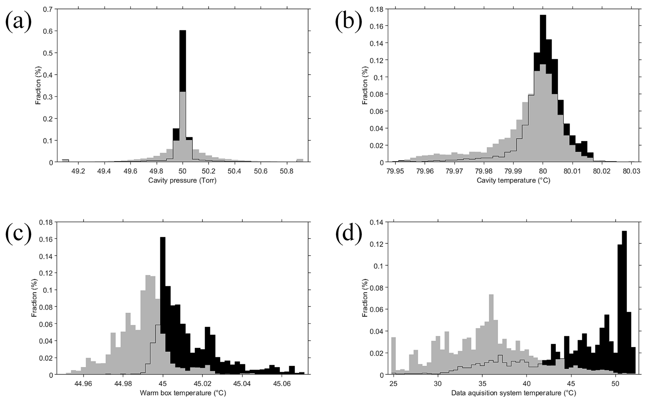
Figure D2CRDS instrument parameters on the ground (black) and during flight (grey) with ULA-IC. (a) Distribution of cavity pressure (Torr), (b) cavity temperature (∘C), (c) warm-box temperature (∘C), and (d) data acquisition system temperature (∘C) on the ground (black) and during flight segments with level or slowly changing altitude (sequence flag 1 or 2). Data are averaged to a 2 s time interval.
Data can be downloaded from https://metclim-lidars.aeris-data.fr/en/homepage/ (last access: 17 June 2021) upon request to the first author of the paper. ERA5 data were downloaded from the Copernicus Climate Change Service (C3S) Climate Data Store (https://doi.org/10.24381/cds.bd0915c6, Hersbach et al., 2018). The IAEA/WMO Global Network of Isotopes in Precipitation (GNIP) is acknowledged for the access to its database accessible at https://nucleus.iaea.org/wiser (last access: 5 July 2021, registration required).
PC coordinated the field campaign and wrote the paper, with contributions from CF, HS, AM, ED, and JT. HS and AS sampled and processed the stable water isotope data. JT calibrated WALI and derived the water vapour profiles. PC, HS, JT, AM, ED, AB, AS, PD, AD, and SR participated in the field campaign. HCSL and all the authors contributed to proofreading of the paper.
The authors declare that they have no conflict of interest.
Publisher's note: Copernicus Publications remains neutral with regard to jurisdictional claims in published maps and institutional affiliations.
Friendly acknowledgements to local authorities of the town of Lathuile Roland Aumaître, Hervé Bourne, Christophe Lambert; instrument providers Florent Arthaud (USMB); Dominique Crucciani for its welcome at the Delta Evasion airfield; ULA pilots Franck Toussaint, Loïc Toussaint, Félix Toussaint; technical assistance Fabienne Maignan and Céline Diana.
This research has been supported by the Agence Nationale de la Recherche via the WAVIL project (grant no. ANR-16-CE01-0009), the Research Council of Norway via the FARLAB project (grant no. 245907), and the ERC-2017-CoG via the ISLAS project (grant no. 773245).
This paper was edited by Heini Wernli and reviewed by two anonymous referees.
Barthlott, C., Corsmeier, U., Meißner, C., Braun, F., and Kottmeier, C.: The influence of mesoscale circulation systems on triggering convective cells over complex terrain, Atmos. Res., 81, 150–175, https://doi.org/10.1016/j.atmosres.2005.11.010, 2006.
Behrendt, A.: Temperature Measurements with Lidar, in: Lidar. Springer Series in Optical Sciences, edited by: Weitkamp, C., Springer, New York, NY, USA, 102, 273–305, https://doi.org/10.1007/0-387-25101-4_10, 2006.
Berkelhammer, M., Noone, D. C., Wong, T. E., Burns, S. P., Knowles, J. F., Kaushik, A., Blanken, P. D., and Williams, M. W.: Convergent approaches to determine an ecosystem's transpiration fraction, Global Biogeochem. Cy., 30, 933–951, https://doi.org/10.1002/2016GB005392, 2016.
Berthier, S., Chazette, P., Couvert, P., Pelon, J., Dulac, F., Thieuleux, F., Moulin, C., and Pain, T.: Desert dust aerosol columnar properties over ocean and continental Africa from Lidar in-Space Technology Experiment (LITE) and Meteosat synergy, J. Geophys. Res., 111, D21202, https://doi.org/10.1029/2005JD006999, 2006.
Chazette, P. and Totems, J.: Mini N2-Raman Lidar onboard ultra-light aircraft for aerosol measurements: Demonstration and extrapolation, Remote Sens., 9, 1226, https://doi.org/10.3390/rs9121226, 2017.
Chazette, P., Couvert, P., Randriamiarisoa, H., Sanak, J., Bonsang, B., Moral, P., Berthier, S. S., Salanave, S., and Toussaint, F.: Three-dimensional survey of pollution during winter in French Alps valleys, Atmos. Environ., 39, 1035–1047, https://doi.org/10.1016/j.atmosenv.2004.10.014, 2005.
Chazette, P., Sanak, J., and Dulac, F.: New approach for aerosol profiling with a lidar onboard an ultralight aircraft: application to the African Monsoon Multidisciplinary Analysis, Environ. Sci. Technol., 41, 8335–8341, https://doi.org/10.1021/es070343y, 2007.
Chazette, P., Dabas, A., Sanak, J., Lardier, M., and Royer, P.: French airborne lidar measurements for Eyjafjallajökull ash plume survey, Atmos. Chem. Phys., 12, 7059–7072, https://doi.org/10.5194/acp-12-7059-2012, 2012.
Chazette, P., Marnas, F., and Totems, J.: The mobile Water vapor Aerosol Raman LIdar and its implication in the framework of the HyMeX and ChArMEx programs: application to a dust transport process, Atmos. Meas. Tech., 7, 1629–1647, https://doi.org/10.5194/amt-7-1629-2014, 2014.
Chazette, P., Totems, J., and Shang, X.: Atmospheric aerosol variability above the Paris Area during the 2015 heat wave – Comparison with the 2003 and 2006 heat waves, Atmos. Environ., 170, 216–233, https://doi.org/10.1016/j.atmosenv.2017.09.055, 2017.
Chazette, P., Totems, J., Baron, A., Flamant, C., and Bony, S.: Trade-wind clouds and aerosols characterized by airborne horizontal lidar measurements during the EUREC4A field campaign, Earth Syst. Sci. Data, 12, 2919–2936, https://doi.org/10.5194/essd-12-2919-2020, 2020.
Craig, H. and Gordon, L. I.: Deuterium and oxygen 18 variations in the ocean and the marine atmosphere, in: Stable Isotopes in Oceanographic Studies and Paleotemperatures, edited by: Tongiorgi, E., Laboratorio di Geologia Nucleare, Pisa, Italy, 1965.
Cui, B. L., Li, X. Y., and Wei, X. H.: Isotope and hydrochemistry reveal evolutionary processes of lake water in Qinghai Lake, J. Great Lakes Res., 42, 580–587, https://doi.org/10.1016/j.jglr.2016.02.007, 2016.
Cunliffe, M., Engel, A., Frka, S., Gašparović, B. Ž., Guitart, C., Murrell, J. C., Salter, M., Stolle, C., Upstill-Goddard, R., and Wurl, O.: Sea surface microlayers: A unified physicochemical and biological perspective of the air-ocean interface, Prog. Oceanogr., 109, 104–116, https://doi.org/10.1016/j.pocean.2012.08.004, 2013.
Danis, P.-A.: Modélisation du fonctionnement thermique, hydrologique et isotopique de systèmes lacustres: sensibilité aux changements climatiques et amélioration des reconstructions paléoclimatiques, HAL Id: tel-00360067, version 1, available at: https://tel.archives-ouvertes.fr/tel-00360067 (last access: 5 November 2020), 2009.
Danis, P. A., Von Grafenstein, U., and Masson-Delmotte, V.: Sensitivity of deep lake temperature to past and future climatic changes: A modeling study for Lac d'Annecy, France, and Ammersee, Germany, J. Geophys. Res.-Atmos., 108, 4609, https://doi.org/10.1029/2003jd003595, 2003.
Dansgaard, W.: Stable isotopes in precipitation, Tellus, 16, 436–468, https://doi.org/10.3402/tellusa.v16i4.8993, 1964.
Demoz, B. B., Collett, J. L., and Daube, B. C.: On the caltech active strand cloudwater collectors, Atmos. Res., 41, 47–62, https://doi.org/10.1016/0169-8095(95)00044-5, 1996.
Drobinski, P., Steinacker, R., Richner, H., Baumann-Stanzer, K., Beffrey, G., Benech, B., Berger, H., Chimani, B., Dabas, A., Dorninger, M., Dürr, B., Flamant, C., Frioud, M., Furger, M., Gröhn, I., Gubser, S., Gutermann, T., Häberli, C., Häller-Scharnhost, E., Jaubert, G., Lothon, M., Mitev, V., Pechinger, U., Piringer, M., Ratheiser, M., Ruffieux, D., Seiz, G., Spatzierer, M., Tschannett, S., Vogt, S., Werner, R., and Zängl, G.: Föhn in the Rhine Valley during MAP: A review of its multiscale dynamics in complex valley geometry, Q. J. R. Meteorol. Soc., 133, 897–916, https://doi.org/10.1002/qj.70, 2007.
Dutton, A., Wilkinson, B. H., Welker, J. M., Bowen, G. J., and Lohmann, K. C.: Spatial distribution and seasonal variation in of modern precipitation and river water across the conterminous USA, Hydrol. Process., 19, 4121–4146, https://doi.org/10.1002/hyp.5876, 2005.
Flamant, C., Drobinski, P., Nance, L., Banta, R., Darby, L., Dusek, J., Hardesty, M., Pelon, J., and Richard, E.: Gap flow in an Alpine valley during a shallow south föhn event: Observations, numerical simulations and hydraulic analogue, Q. J. R. Meteorol. Soc., 128, 1173–1210, https://doi.org/10.1256/003590002320373256, 2002.
Gat, J. R.: Oxygen and hydrogen isotopes in the hydrologic cycle, Annu. Rev. Earth Planet. Sci., 24, 225–262, https://doi.org/10.1146/annurev.earth.24.1.225, 1996.
Gat, J. R.: Atmospheric water balance-the isotopic perspective, Hydrol. Process., 14, 1357–1369, 2000.
Gat, J. R.: Isotope Hydrology – A study of the water cycle, edited by: Wei, T. K., Imperial College Press, World Scientific Publishing Co., Singapore, 2010.
Gat, J. R., Bowser, C. J., and Kendall, C.: The contribution of evaporation from the Great Lakes to the continental atmosphere: estimate based on stable isotope data, Geophys. Res. Lett., 21, 557–560, https://doi.org/10.1029/94GL00069, 1994.
Gibson, J. J. and Edwards, T. W. D.: Regional water balance trends and evaporation-transpiration partitioning from a stable isotope survey of lakes in northern Canada, Global Biogeochem. Cy., 16, 10-1–10-14, https://doi.org/10.1029/2001gb001839, 2002.
Graf, P., Wernli, H., Pfahl, S., and Sodemann, H.: A new interpretative framework for below-cloud effects on stable water isotopes in vapour and rain, Atmos. Chem. Phys., 19, 747–765, https://doi.org/10.5194/acp-19-747-2019, 2019.
Griffis, T. J., Wood, J. D., Baker, J. M., Lee, X., Xiao, K., Chen, Z., Welp, L. R., Schultz, N. M., Gorski, G., Chen, M., and Nieber, J.: Investigating the source, transport, and isotope composition of water vapor in the planetary boundary layer, Atmos. Chem. Phys., 16, 5139–5157, https://doi.org/10.5194/acp-16-5139-2016, 2016.
Gupta, H. V., Kling, H., Yilmaz, K. K., and Martinez, G. F.: Decomposition of the mean squared error and NSE performance criteria: Implications for improving hydrological modelling, J. Hydrol., 377, 80–91, https://doi.org/10.1016/j.jhydrol.2009.08.003, 2009.
He, H. and Smith, R. B.: Stable isotope composition of water vapor in the atmospheric boundary layer above the forests of New England, J. Geophys. Res.-Atmos., 104, 11657–11673, https://doi.org/10.1029/1999JD900080, 1999.
Herrmann, H.: Kinetics of Aqueous Phase Reactions Relevant for Atmospheric Chemistry, Chem. Rev., 103, 4691–4716, https://doi.org/10.1021/cr020658q, 2003.
Hersbach, H., Bell, B., Berrisford, P., Biavati, G., Horányi, A., Muñoz Sabater, J., Nicolas, J., Peubey, C., Radu, R., Rozum, I., Schepers, D., Simmons, A., Soci, C., Dee, D., and Thépaut, J.-N.: ERA5 hourly data on pressure levels from 1979 to present, Copernicus Climate Change Service (C3S) Climate Data Store (CDS) [data set], https://doi.org/10.24381/cds.bd0915c6, 2018.
IAEA: Reference Sheet for VSMOW2 and SLAP2 international measurement standards, International Atomic Energy Agency, Vienna, Austria, 5 pp., available at: https://nucleus.iaea.org/sites/ReferenceMaterials/Shared Documents/ReferenceMaterials/StableIsotopes/VSMOW2/VSMOW2_SLAP2.pdf (last access: 8 July 2021), 2009.
Jasechko, S., Sharp, Z. D., Gibson, J. J., Birks, S. J., Yi, Y., and Fawcett, P. J.: Terrestrial water fluxes dominated by transpiration, Nature, 496, 347–350, https://doi.org/10.1038/nature11983, 2013.
Kendall, C. and Coplen, T. B.: Distribution of oxygen-18 and deuteriun in river waters across the United States, Hydrol. Process., 15, 1363–1393, https://doi.org/10.1002/hyp.217, 2001.
Koscielny, A. J., Doviak, R. J., and Zrnic, D. S.: An Evaluation of the Accuracy of Some Radar Wind Profiling Techniques, J. Atmos. Ocean. Technol., 1, 309–320, https://doi.org/10.1175/1520-0426(1984)001<0309:AEOTAO>2.0.CO;2, 1984.
Kottmeier, C., Kalthoff, N., Barthlott, C., Corsmeier, U., Van Baelen, J., Behrendt, A., Behrendt, R., Blyth, A., Coulter, R., Crewell, S., Di Girolamo, P., Dorninger, M., Flamant, C., Foken, T., Hagen, M., Hauck, C., Höller, H., Konow, H., Kunz, M., Mahlke, H., Mobbs, S., Richard, E., Steinacker, R., Weckwerth, T., Wieser, A., and Wulfmeyer, V.: Mechanisms initiating deep convection over complex terrain during COPS, Meteorol. Z., 17, 931–948, https://doi.org/10.1127/0941-2948/2008/0348, 2008.
Lesouëf, D., Gheusi, F., Chazette, P., Delmas, R., and Sanak, J.: Low Tropospheric Layers Over Reunion Island in Lidar-Derived Observations and a High-Resolution Model, Bound.-Lay. Meteorol., 149, 425–453, https://doi.org/10.1007/s10546-013-9851-9, 2013.
Majoube, M.: Fractionnement en oxygène 18 et en deutérium entre l'eau et sa vapeur, J. Chim. Phys., 68, 1423–1436, https://doi.org/10.1051/jcp/1971681423, 1971.
Mayr, G. J., Armi, L., Gohm, A., Zängl, G., Durran, D. R., Flamant, C., Gaberšek, S., Mobbs, S., Ross, A., and Weissmann, M.: Gap flows: Results from the Mesoscale Alpine Programme, Q. J. R. Meteorol. Soc., 133, 881–896, https://doi.org/10.1002/qj.66, 2007.
Noone, D.: Pairing measurements of the water vapor isotope ratio with humidity to deduce atmospheric moistening and dehydration in the tropical midtroposphere, J. Climate, 25, 4476–4494, https://doi.org/10.1175/JCLI-D-11-00582.1, 2012.
Platt, C. M. R.: Lidar Observation of a Mixed-Phase Altostratus Cloud, J. Appl. Meteorol., 16, 339–345, https://doi.org/10.1175/1520-0450(1977)016<0339:looamp>2.0.co;2, 1977.
Raut, J.-C. and Chazette, P.: Assessment of vertically-resolved PM10 from mobile lidar observations, Atmos. Chem. Phys., 9, 8617–8638, https://doi.org/10.5194/acp-9-8617-2009, 2009.
Salmon, O. E., Welp, L. R., Baldwin, M. E., Hajny, K. D., Stirm, B. H., and Shepson, P. B.: Vertical profile observations of water vapor deuterium excess in the lower troposphere, Atmos. Chem. Phys., 19, 11525–11543, https://doi.org/10.5194/acp-19-11525-2019, 2019.
Sodemann, H., Aemisegger, F., Pfahl, S., Bitter, M., Corsmeier, U., Feuerle, T., Graf, P., Hankers, R., Hsiao, G., Schulz, H., Wieser, A., and Wernli, H.: The stable isotopic composition of water vapour above Corsica during the HyMeX SOP1 campaign: insight into vertical mixing processes from lower-tropospheric survey flights, Atmos. Chem. Phys., 17, 6125–6151, https://doi.org/10.5194/acp-17-6125-2017, 2017.
Steen-Larsen, H. C., Johnsen, S. J., Masson-Delmotte, V., Stenni, B., Risi, C., Sodemann, H., Balslev-Clausen, D., Blunier, T., Dahl-Jensen, D., Ellehøj, M. D., Falourd, S., Grindsted, A., Gkinis, V., Jouzel, J., Popp, T., Sheldon, S., Simonsen, S. B., Sjolte, J., Steffensen, J. P., Sperlich, P., Sveinbjörnsdóttir, A. E., Vinther, B. M., and White, J. W. C.: Continuous monitoring of summer surface water vapor isotopic composition above the Greenland Ice Sheet, Atmos. Chem. Phys., 13, 4815–4828, https://doi.org/10.5194/acp-13-4815-2013, 2013.
Steen-Larsen, H. C., Sveinbjörnsdottir, A. E., Peters, A. J., Masson-Delmotte, V., Guishard, M. P., Hsiao, G., Jouzel, J., Noone, D., Warren, J. K., and White, J. W. C.: Climatic controls on water vapor deuterium excess in the marine boundary layer of the North Atlantic based on 500 days of in situ, continuous measurements, Atmos. Chem. Phys., 14, 7741–7756, https://doi.org/10.5194/acp-14-7741-2014, 2014.
Totems, J., Chazette, P., and Raut, J.: Accuracy of current Arctic springtime water vapour estimates, assessed by Raman lidar, Q. J. R. Meteorol. Soc., 145, 1234–1249, https://doi.org/10.1002/qj.3492, 2019.
Weng, Y., Touzeau, A., and Sodemann, H.: Correcting the impact of the isotope composition on the mixing ratio dependency of water vapour isotope measurements with cavity ring-down spectrometers, Atmos. Meas. Tech., 13, 3167–3190, https://doi.org/10.5194/amt-13-3167-2020, 2020.
Worden, J., Noone, D., Bowman, K., Beer, R., Eldering, A., Fisher, B., Gunson, M., Goldman, A., Herman, R., Kulawik, S. S., Lampel, M., Osterman, G., Rinsland, C., Rodgers, C., Sander, S., Shephard, M., Webster, C. R., and Worden, H.: Importance of rain evaporation and continental convection in the tropical water cycle, Nature, 445, 528–532, https://doi.org/10.1038/nature05508, 2007.
- Abstract
- Introduction
- L-WAIVE experimental strategy
- Instrumental setup on each platform
- Meteorological conditions during L-WAIVE
- Water vapour isotope during L-WAIVE
- Synthesis and discussion
- Conclusion
- Appendix A: L-WAIVE data availability
- Appendix B: Ultra-light aircraft flights description
- Appendix C: Water vapour stable isotopes interpretive framework
- Appendix D: Water isotope data processing
- Data availability
- Author contributions
- Competing interests
- Disclaimer
- Acknowledgements
- Financial support
- Review statement
- References