Modelling Phosphorus Export from Humid Subtropical Agricultural Fields: A Case Study Using the HSPF Model in the Mississippi Alluvial Plain

Diaz-Ramirez J; Martin JL; William HM

doi:10.4172/2157-7617.1000162

ISSN: 2157-7617

Journal of Earth Science & Climatic Change

Like us on:

Make the best use of Scientific Research and information from our 700+ peer reviewed, Open Access Journals that operates with the help of 50,000+ Editorial Board Members and esteemed reviewers and 1000+ Scientific associations in Medical, Clinical, Pharmaceutical, Engineering, Technology and Management Fields.

Meet Inspiring Speakers and Experts at our 3000+ Global Conferenceseries Events with over 600+ Conferences, 1200+ Symposiums and 1200+ Workshops on Medical, Pharma, Engineering, Science, Technology and Business

Modelling Phosphorus Export from Humid Subtropical Agricultural Fields: A Case Study Using the HSPF Model in the Mississippi Alluvial Plain

*Diaz-Ramirez J^1, Martin JL² and William HM³**
¹Mississippi River Research Center, Alcorn State University, Alcorn State, USA
²Department of Civil and Environmental Engineering, Mississippi State University, USA
³Geosystems Research Institute, Mississippi State University, USA
Corresponding Author :	Diaz-Ramirez J Director, Mississippi River Research Center Alcorn State University, Alcorn State, USA E-mail: jdiaz@alcorn.edu
Received August 17, 2013; Accepted September 20, 2013; Published September 28, 2013
Citation: Diaz-Ramirez J, Martin JL, William HM (2013) Modelling Phosphorus Export from Humid Subtropical Agricultural Fields: A Case Study Using the HSPF Model in the Mississippi Alluvial Plain. J Earth Sci Clim Change 4:162. doi:10.4172/2157-7617.1000162
Copyright: © 2013 Diaz-Ramirez J, et al. This is an open-access article distributed under the terms of the Creative Commons Attribution License, which permits unrestricted use, distribution, and reproduction in any medium, provided the original author and source are credited.

Visit for more related articles at Journal of Earth Science & Climatic Change

View PDF Download PDF Tables & Figures

Abstract

This research used extensive field data collected during the 1990’s by a consortium of federal, state, local, and university personnel in agricultural areas in the Mississippi Delta region to evaluate runoff, soil erosion, and nutrient losses. Agricultural phosphorus export modelling was performed on Deep Hollow watershed (11.29 ha) using the
Hydrological Simulation Program FORTRAN – HSPF to demonstrate the usefulness of the continuous processesbased model for a farm scale drainage area in the Mississippi Delta region. The main goal of this study was to evaluate the ability of HSPF to simulate storm, seasonal, and long-term runoff, sediment, and phosphorus export at the farm scale in Mississippi. The model was spatially divided into six hydrologic respond units based on similarity of land cover and soil characteristics. Rainfall and other climate time series were setup every 15-minutes and the model results were output at the same time step. Agricultural field operations (tillage, cultivation, harvest, fertilization) were incorporated into the HSPF model using the special actions module. Phosphorus simulations were accomplished using the AGCHEMPHOS module. Phosphorus adsorption and desorption were simulated by the Freundlich method. Model outputs: runoff, sediment load, dissolved & total phosphorus loads were evaluated against observed data from storm, seasonal, and long-term periods. Collected storm-event data at the drainage area outlet were available for runoff (69 events), suspended sediment load (40 events), and phosphorus loads (23 events) from 1997 to 1999. The model was calibrated using available data from 1998 to 1999 and validated using field data in 1999. All the parameter values used in this assessment were in the range provided by HSPF model developers or found in the literature. Simulated runoff values showed very good agreements to storm, monthly, and annual basis. In analyzing simulated sediment load export values, storm type steps yielded poor performance, but HSPF produced good seasonal and annual sediment load values. Simulated dissolved phosphorus (DP) loads were better at long-term time steps than storm-by-storm periods. HSPF total phosphorus (TP) loads were better at simulating long-term periods than storm-by-storm time steps. In conclusion, HSPF runoff algorithms are very robust at any time scales from storm to annual periods and sediment and phosphorus modules are very comprehensive for seasonal and annual time steps at the farm scale.

Keywords

Phosphorus; Subtropical; Delta; Drainage; Rainfall; Climate

Introduction

Excess nutrients are known as a primary problem facing Gulf of Mexico estuaries and coastal waters, leading to nuisance algal blooms, depletion of dissolved oxygen, and other water quality impairments. The Lower Mississippi river watershed was ecologically transformed from millions of hectares of forest to agricultural uses in the last century. In addition, the floodplain connectivity was lost by hundredths of kilometres of levees. The lack of conservation practices in agricultural land uses yields high amounts of sediments, nutrients, and pesticides. Groundwater mining in the region has resulted in decreased groundwater levels and frequently a reduced availability of groundwater supplies, which negatively impacts agriculture and other uses. The reduced groundwater levels have also resulted in a lack of hydrologic connectivity with some surface water streams, such as the sunflower river in the Mississippi delta, resulting in the reduction or elimination of base flows and consequent water quality impairments, such as hypoxia. Nutrient load reduction from and nutrient criteria development for the Lower Mississippi Valley Alluvium are priority issues for a variety of agencies and organizations and the public. For example, a key component of the Gulf Hypoxia Action Plan calls for the development of state nutrient reduction strategies for those states with significant contributions of nitrogen and phosphorus to the Gulf.

Soil and phosphorus exported from agricultural fields into water bodies in the Mississippi Delta region is a major environmental concern by local, state, and federal agencies. Soil and phosphorus losses encourage siltation and eutrophication in Gulf of Mexico waters. Sedimentation plays a major role in waterborne transportation. Sediment management is very expensive in channels and harbours due to dragging costs to remove sediments. The aquatic ecosystem is affected by excess of nutrient loads promoting low dissolved oxygen values. In particular, phosphorus is an environmental concern because it is generally the limiting nutrient in natural ecosystems. Soil erosion is an important mechanism of phosphorus loss. Phosphorus can be in the water column as dissolved or attached to sediment particles. The processes associated to sediment and phosphorus transport from agricultural fields are complex due to crop management including tillage, fertilization, and harvest. Approaches to better understand the processes of runoff, soil erosion, and phosphorus loss from agricultural watersheds can range from field experiments (including plots, farm, and small & large drainage areas) to modelling tools (from empirical to processes based methods). The temporal scale in analyzing and reporting rainfall-runoff, soil erosion, and phosphorus losses varies greatly between storm and annual values.

There are several computer tools that simulate hydrology, soil erosion, and nutrient transport at the field and watershed scales. Most common tools used in USA sponsored by federal agencies include the Hydrological Simulation Program FORTRAN-HSPF [1], the Soil and Water Assessment Tool-SWAT [2], the Agricultural Policy/ Environmental eXtender-APEX [3], and the Annualized Agricultural Non-Point Source-AnnAGNPS [4]. These computer programs have marked differences in mathematical algorithm architecture, input data requirements, pre & post processing interfaces, and temporal & spatial scale applications.

State agencies are presently developing nutrient criteria, which when implemented would be expected to result in requirements for nutrient load reductions to remove identified impairments, such as for the nearly 7,000 water bodies of the U.S. presently listed (303(d) listed impairments) as not meeting water quality standards due to nutrients. Effective implementation of nutrient load reductions requires that analytical tools be available to accurately estimate loads from watersheds and water bodies as a function of hydrologic conditions and alternative management practices. Hydrologic models are available that could be used to estimate relationships among climate, soil characteristics, land practices, and nutrient runoff. Hydrologic models could be used, for example, to estimate nutrient loads from watersheds under existing conditions and conditions following implementation of best management practices (BMPs) in order to estimate potential load reductions. Hydrologic models can also be used to aid in the site selection and design of BMPs.

During the 1990’s, a research team of federal, state, local, and university personnel carried out studies at the field-scale in agricultural areas in the Mississippi Delta region to evaluate runoff, soil erosion, nutrient losses [5]. In addition, BMPs were evaluated to compute efficiencies in trapping sediments and nutrients at the field-scale. One of the intensive study areas was Deep Hollow. The main goal of this study was to test the capability of the HSPF model to predict storm, seasonal, and long-term runoff, sediment, and phosphorus transport at the farm scale in the Deep Hollow drainage area, Mississippi.

Materials and Methods

Study area

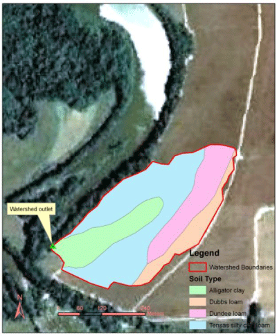
This study evaluated the HSPF model in the Deep Hollow drainage area, Mississippi (Figure 1). The 11.29-ha drainage area is a flat area with a mean slope of 0.5%. Table 1 shows land cover and hydrologic soil group (HSG) distribution in the study area. The Deep Hollow farm was cropped with soybeans and cotton. Winter wheat was planted during the off season in the entire farm. The majority of the soils presents high runoff potential (HSGD=67.6%).

The HSPF model: The Hydrologic Simulation Program- FORTRAN (HSPF) model [1] computes the movement of water through a complete hydrologic cycle-rainfall, evapotranspiration, runoff, infiltration, and flow through the ground-and the associated transport of constituents with that flow. It represents a watershed as a collection of land segments and channels (reaches). The land segments, either pervious or impervious, are connected to other land segments or to channel reaches, which can function as either streams or reservoirs. Model time steps vary from minutes to daily depending of available climate time series data. The HSPF model also computes the transport and kinetics of multiple water quality constituents, including temperature, sediment, nutrients, and pesticides. As such it presents a nearly complete package for modelling hydrology and water quality of a watershed. A more complete description of features and capabilities can be found in the HSPF user’s manual [1].

Before running HSPF, the watershed area must be delineated into homogeneous land areas called Hydrologic Response Units (HRUs). For each HRU the combination of weather, soil, land use, topographic and geologic properties is unique, giving rise to its “semi-distributed” model structure. HRUs can be impervious or pervious areas, which are modelled independently. Each HRU requires input data such as rainfall, temperature, potential evapotranspiration, and parameters related to land use, soil characteristics, and agricultural practices to simulate hydrology, sediments, nutrients and pesticides [6]. HRUs outputs can be linked among them (lateral connection) or connected to the nearest channel. Most of the HSPF applications use independent HRUs connected to the nearest reach. This simplification makes the HSPF model implementation/application easy and fast; however, some physical information among HRUs processes can be lost.

Some versions of HSPF can be run in standalone mode, but the EPA-supported version is run through a BASINS interface, WinHSPF [7]. The rainfall-runoff model HSPF requires specific inputs that BASINS can generate. Watershed delineation tools within BASINS enable the user to automatically or manually generate a watershed drainage network and sub-networks, each consisting of land segments and receiving water reaches. BASINS (or its utility program, WDMUtil) creates a binary file with a “.wdm” extension to storage input time-series information such as rainfall, wind speed, and temperature for stations in or near the watershed. HSPF reads these text and binary files and constructs two more files, an ASCII run control file (with a “.uci” extension) and a binary input/output file (with a “.wdm” extension). These files can be manipulated by the user and used in all subsequent simulations. Expert HSPF users can create specific HSPF applications without the use of BASINS interface or any other graphical user interface. Particularly, this is useful in developing models from small areas with few land segments and reaches.

For the purposes of this research, a summary on the hydrology, sediment, and phosphorus modules are provided below. This summary is focused on HSPF processes over pervious areas where channel processes are negligible.

HSPF hydrology: Algorithms for hydrological simulation in HSPF originated from the Stanford Watershed Model [8]. Hydrological simulation in HSPF consists of five storage classes (interception, upper zone, lower zone, base flow, and deep percolation), each allowing different types of inflow and outflow. Inflows and outflows are simulated in HSPF as water-balance accounting. Each pervious land segment considers the following processes: interception, evapotranspiration, surface detention, surface runoff, infiltration, shallow subsurface flow (interflow), base flow, and deep percolation [6]. Surface detention and surface runoff are the only components simulated in impervious areas.

Interception is defined by the model as the volume of water captured by an area’s vegetative cover. Each type of vegetative cover is assigned a constant maximum volume. If this volume is exceeded, the water will be subject to one of the other pathways. Rainfall enters into the volume and evaporation takes away from the volume. The maximum volume can be adjusted by month, which is especially valuable for crop areas. Infiltration is calculated by means a negative power relationship. Both Hortonian and saturation excess overland flow can be simulated in HSPF. The equation used by the model to represent overland flow is an altered version of Manning’s equation. The area and hydraulic radius terms have simply been replaced with a depth term. Because overland flow is horizontal flow, the depth is often very small. A larger roughness coefficient also exists because of the slight depth encountered in overland flow compared to channel flow. A portion of surface runoff becomes upper-zone storage, simulating both depression storage and upper-soil storage, and the balance becomes overland flow. Infiltrated water can become interflow and reach the nearest channel. Interflow moves slower than surface runoff and stretches the output hydrograph. Infiltrated water that does not go into interflow or lower-zone storage is finally placed in the active groundwater storage. Active groundwater storage is divided into deep percolation and base flow. Deep percolation is simulated as a sink. Base flow is simulated using linear and power equations. HSPF is not a groundwater model, as many of the principles associated with such models are extraordinarily complex. Many of these principles are simplified or basic assumptions about groundwater are made to allow hydrologic models such as HSPF to account for groundwater.

Actual evapotranspiration is simulated in response to the input value of potential evapotranspiration. Water evaporates first from the riparian vegetation (wetlands). Further actual evapotranspiration is satisfied sequentially by interception storage, upper zone storage, active ground water, and lower-zone storage where each storage has a different resistance to evaporation. In this way the maximum potential of each storage is depleted either when all storages have contributed their maximum amount to evapotranspiration or until the potential evapotranspiration has been fully satisfied.

HSPF sediments: The equations applied for modelling the production and removal of sediments are based on ARM and NPS predecessor models [6]. These equations were originated from a sediment model created by [9] and influenced by Meyer and Onstad [10,11]. Whereas HSPF does not use the Universal Soil Loss Equation- USLE [12] specifically, several concepts of both models are analogous. In previous areas, removal of sediments by water is simulated as wash off of detached sediment due to the rainfall and other sediment scour from the soil matrix. Sediment is detached from the surface pervious areas as a function of rainfall intensity, land cover, land management practices, and soil detachment properties [6]. In HSPF two situations can arise involving detached sediment: either sediment limiting or transport limiting. Sediment limiting is when the generation and accumulation parameters have major impact. This occurs when the capacity for removing detached sediment exceeds the amount of detached sediment storage. When the capacity is less than the available storage, it is considered transport limiting. Transport limiting means that the sediment transport parameters have primary impact. Sediments move from the detached sediment store or from scouring of the soil matrix to the stream. They reattach only on dry days. The contribution from each source is determined by the amount of overland flow, which is determined by hydrology simulation [1].

HSPF phosphorus: Nutrient modelling can be significantly more difficult than either hydrology or sediments due to the complexities of the processes involved. In addition, hydrological and sediment processes are required to build a nutrient model. The majority of the nutrient processes in HSPF are derived from the Non-Point Source Model and HSP QUALITY [1]. Modelling nutrients in HSPF can be approached in two ways: treating it at a generalized constituent (PQUAL module) with empirically-based equations or using processesbased subroutines (AGCHEM module) such as PHOS (phosphorus) or NITR (nitrogen). Although this AGCHEM subroutine is often more accurate and realistic, the data requirements for these algorithms are stringent. For example, meteorological data such as cloud cover and wind speed are needed in order for them to run; initial nutrient values are needed for each of the four soil storages; depth of each soil layer is required. This study used the AGCHEM-PHOS algorithms to simulate phosphorus fate in the Deep Hollow drainage area. For this reason, a summary on the HSPF-PHOS processes over pervious areas is provided next.

In HSPF, behaviour of phosphorus from agricultural fields can be simulated using a yield-based nutrient uptake AGCHEM-PHOS algorithm. When the AGCHEM-PHOS module is selected, the soil matrix is divided in four layers (surface, upper, lower, and groundwater) where phosphorus reactions take place in each compartment. This algorithm simulates the transport, plant uptake, and transformations (adsorption/desorption, immobilization, and mineralization) of the different species of phosphorus. HSPF-PHOS simulates phosphorus as sediment-attached, dissolved in surface runoff, and as concentrations in the interflow and ground water compartments. Phosphorus adsorption and desorption can be simulated by either first-order kinetics or by the Freundlich method. Mineralization, immobilization, and plant uptake reactions are simulated using temperature dependent, first-order kinetics. Detailed inputs of agricultural farm management activities including tillage, cultivation, fertilization, and harvest are handled through the model’s special actions module.

Model evaluation

Statistical methods: Several different numerical criteria were used to evaluate the simulated versus the observed variables at storm, monthly, and annual levels. They are as follows: the relative error (RE), the root mean square error (RMSE), the coefficient of determination (R²), and the Nash-Sutcliffe coefficient (NS). Scatter plots were used to evaluate observed versus simulated variables. This section presents a summary of the meaning of the numerical measures used in this study. Equations of these numerical measures can be found in Moriasi [13].

Relative error: The relative error is the absolute error divided by the magnitude of the exact value. The percent error is the relative error expressed in terms of per 100.

Root mean square error: The root mean square error (RMSE) is a frequently-used measure of the differences between values predicted by a model or an estimator and the values actually observed from the thing being modelled or estimated. RMSE is a good measure of precision. These individual differences are also called residuals, and the RMSE serves to aggregate them into a single measure of predictive power.

Coefficient of determination: The coefficient of determination (R²) describes the degree of collinearity between simulated and measured data. R² describes the proportion of the variance in measured data explained by the model. R² ranges from 0 to 1, with higher values indicating less error variance, and typically values greater than 0.5 are considered acceptable.

Nash-sutcliffe coefficient: The Nash-Sutcliffe is a normalized statistic that determines the relative magnitude of the residual variance compared to the measured data variance (Nash and Sutcliffe, 1970). NSE indicates how well the plot of observed versus simulated data fits the 1:1 line. NSE ranges between -∞ and 1.0, with NSE=1.0 being the optimal value. Values between 0.0 and 1.0 are generally viewed as acceptable levels of performance, whereas values<0.0 indicates that the mean observed value is a better predictor than the simulated value, which indicates unacceptable performance [13].

Approach for model calibration and validation

The Deep Hollow drainage area was subdivided into six hydrologic respond units - HRUs based on similarity of land cover and hydrologic soil groups -HSGs (Table 1). Area values from each HRU were taken from Yuan et al. (2001). Soil property information used in this study was extracted from the USDA SSURGO database (USDA-NRCS, 2012). Detailed crop management information (tillage, fertilization, harvest) can be found in [14,15].

USGS site-collected 15-minute rainfall data were used in this study. Hourly climate time series (maximum and minimum air temperatures, dew point, wind, solar ration, and cloud cover) were extracted from the NOAA Greenwood Leflore Airport station, located 16.7 km from the drainage area. Hourly potential evapotranspiration was calculated using temperature data from the Greenwood Leflore Airport station and the Hamon method [16] implemented in the BASINS program [17]. All climate data were converted to 15-minute time series by equally dividing the hourly values.

The study area did not have a define channel and no channel process were simulated in HSPF. In other words, only pervious land segment algorithms (water budget and runoff components; sediment production and removal; and phosphorus fate & runoff) were used in this research. Phosphorus transformations were simulated using the PHOS AGCHEM module. The HSPF model time step and outputs were set to15 minutes. Model outputs were evaluated against runoff, total suspended sediments, and dissolved & total phosphorus time series collected at the outlet of the drainage area by USGS (USGS 0728711620 Unknown Lake Tributary No 2 Near Sidon, MS).

The calibration was performed from January 1, 1997 to December 31, 1998. Due to the small size of the drainage area (no base flow processes), the results of the HSPF hydrology simulation are presented by rainfall events. In attempts to increase the confidence in the HSPF simulations, validation was performed using the USGS runoff, sediments, and phosphorus data and on site precipitation time series from January 1, 1999 to December 31, 1999. For the validation processes, the HSPF parameters were not manipulated.

Criteria for evaluating model performance depend on the process simulated (flow, sediments, pesticide, or water quality). To date, modelling professionals (developers and users) have not reached consensus about which criteria is best for evaluating model performance [18,19]. HSPF calibration and validation procedures can be found in [19]. Watershed model evaluation guidelines based on performance ratings can be found in [19] and [13]. These ratings are suggested for daily and long-term time steps. No specific performance ratings by constituent were found in the literature. Table 2 shows the criteria and performance ratings used in this research.

Results

Hydrologic processes

Runoff calibration: Table 3 shows the adjusted parameter values for the calibration. The INFILT parameter is one that drives the flow diversion from surface runoff to infiltration. The INFILT values found in this application were in the range of each hydrologic soil group by polygon. Monthly adjustments were made to the following parameters: INTERCEP, NSUR, and LZETP. Table 4 shows the monthly values for the specified parameters.

The lower zone nominal soil moisture storage (LZSN) is related to precipitation patterns and soil characteristics of the region. The INFILT parameter controls the overall division of the available moisture from precipitation into surface and subsurface flow and storage components. Higher INFILT values will produce more water in the lower zone and groundwater, and result in higher base flow. INFILT is primarily a function of soil characteristics. The length of assumed overland flow plane (LSUR) parameter approximates the average length of travel for water to reach the stream reach, or any drainage path that quickly deliver the water to the stream. The (SLSUR) parameter is simply the average slope of the assumed overland flow path.

The nominal upper zone soil moisture storage (UZSN) parameter is related to land surface characteristics, topography, and LZSN. Due to the high percentage of agriculture on site the values are increased over the months of the growing period. The Manning’s n for overland flow (NSUR) parameter uses monthly values reflecting the seasonal changes in land surface conditions depending on cropping and tillage practices. The index to lower zone evapotranspiration (LZETP) parameter is a coefficient that defines evapotranspiration opportunity. During growing season the LZETP parameter will typically have larger values. Monthly parameter values calibrated in this study were homogenous across the land cover but different month by month, reflecting the crop growing changes.

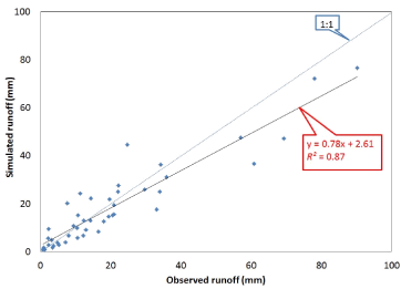
Figure 2 shows the comparison for the observed versus simulated flows (mm) by event for the calibration period. The simulated flow values were overall lower than the observed USGS flow data. The model tended to under predict high runoff events (runoff values greater than 50 mm).

Table 5 shows the observed and simulated flow values. The table includes the relative error (RE) of runoff values by storm event. It can be seen that overall the simulated flow values were below the observed data by approximately 9.04%. Over the calibration time period (1997- 1998) there were 45 rainfall events. The average length of the 45 rainfall events was 550 min, ranging from 60 to 1665 min. Of the 45 simulated events six events fall into the +/- 10% RE range. There were 15 events in the +/- 20% RE range and 25 events in the +/- 30% RE range. The average relative error for the simulated storm events was 8.57% for the calibration period. The R² value of 0.87 was a very good fit for storm event evaluations. The Nash-Sutcliffe value of 0.85 is also a very good value for the hydrology calibration. In general, all the evaluation results were very good for the calibration period.

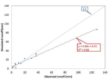
Runoff validation: Figure 3 shows the comparison for the observed versus simulated runoff (mm) by event for the validation time period (1999). In the validation period, there was a tendency of under predict high runoff events by HSPF. The slope of the linear regression in the validation period (0.66) was lower than the one computed in the calibration period (0.78).

Table 6 shows the observed and simulated flows for the validation events. The table shows the simulated flow values were approximately 14.4% less than the observed flow data. Over the validation time period (1999) there were 15 rainfall events. The average length of the 15 rainfall events was 646 min, ranging from 180 to 1710 min. Of the 15 simulated events none event fall into the +/- 10% RE range. There were five events in the +/- 20% RE range and seven events in the +/- 30% RE range. The average relative error for the simulated storm events (RE) was 0.44% for the validation period. The coefficient of determination (R²) value for the validation period was at a great level of 0.98. The Nash-Sutcliffe (NS) value of 0.86 reinforced the validation of the hydrology calibration. The R² and NS for the validation period were much higher than the ones computed in the calibration period. The RMSE for the validation period (44.57 mm) was slightly lower than the one yielded in the calibration period (54.14 mm). The validation data covered a similar runoff range as data used in the calibration period.

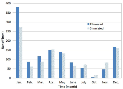
Seasonal and long-term runoff performance: Table 7 depicts simulated and observed total runoff values by month from 1997 to 1999. In total, 60 runoff events were evaluated in this study. January yielded 25% of the total events with the largest amount of runoff. There was no report on rainfall-runoff events in August and September. Discrepancies between observed and simulated runoff values ranged from 1.22% in April to 231.58% in October. Although the largest discrepancy was computed in October, flow values were the lowest ones used in this study. On average, simulated runoff values were lower by 10.53% than observed monthly values. Six out of 10 months were under predicted by the HSPF model. The R² and NS goodness-of-fit values of 0.94 and 0.84, respectively were very good indications of the robustness of the HSPF model in simulating rainfall-runoff processes at the farm scale in the Mississippi Delta region. Figure 4 shows that the model followed close the different runoff seasons in the study area.

Soil erosion processes

Calibration of suspended sediment loads: Table 8 depicts calibrated soil erosion parameters by soil type. The HSPF parameters adjusted throughout the calibration included parameters for estimating the production and reduction of detached sediment on pervious land. The adjusted parameters include: Supporting Management Practice Factor (SMPF), coefficient in the soil detachment equation (KRER), exponent in the soil detachment equation (JRER), and the fraction by which detached sediment storage decreases each day during non storm periods (AFFIX). The KRER parameter values were obtained from the SSURGO database. Other parameters adjusted during calibration were for estimating the sediment removal from the previous land by wash off erosion processes. They consisted of: coefficient in the soil wash off or transport equation (KSER), and exponent in the soil wash off equation (JSER). HSPF values of soil erosion parameters found in this application are in the range suggested by model developers [20].

The cover parameter values for soybean, cotton, and winter wheat in Table 9 were initially extracted from Tables 8 and 10 in [21] and then adjusted. Calibrated parameter values vary monthly due to crop growth and season. Note that cover values were lumped across the different land covers due to lack of specific data for the study area.

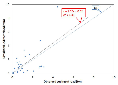
Table 10 depicts the observed and simulated suspended sediment loading values by storm events. The table includes the relative error (RE) between simulated and observed values by rainfall event. Over the calibration time period (1997-1998) there were 29 rainfall events with observed suspended sediment data. Of the 29 simulated events, seven events were into the +/- 50% RE range. There was almost an even ratio between over predicted (14 events) and under predicted (15 events) sediment loads by HSPF. The average relative error for the simulated suspended sediments for the 29 storm events was only 27.04% for the calibration period, indicating an over prediction by the model. The R² value of 0.39 showed a low correlation between observed and simulated sediment load values. However, if the largest observed value (5/29/1998) is taken off the analysis, the R² decreased to 0.12. Using all of the 29 events, the Nash-Sutcliffe (NS) value was -0.87. This negative NS value indicated that the mean observed value was a better predictor than the simulated value, which indicated unacceptable performance. Taking off the largest value collected in 5/29/1998, the recomputed NS figure (-0.59) was not much different of the one using the entire time series. In other words, the NS goodness-of-fit was less sensitive to values out of the trend than the R². This particular study showed the robustness of the NS compared to the R². It can be seen that overall the simulated suspended sediment load values were above the observed data by only 10.28%.

Figure 5 shows observed and simulated suspended sediment loads by storm events. Results were widely scattered around the 1:1 line. It is clear that the model over predicted the largest value by around twice the observed one. The slope value (1.09) of the linear regression equation showed a slightly over prediction by the model. This study’s correlation value and linear fit are similar to ones found by [14] using AnnAGNPS (R²=0.5 and y=1.05x). However these correlations are not fully comparable because model applications used different time intervals; AnnAGNPS application ran from October 1996 to September 1999 and HSPF calibration ran from January 1997 to December 1998.

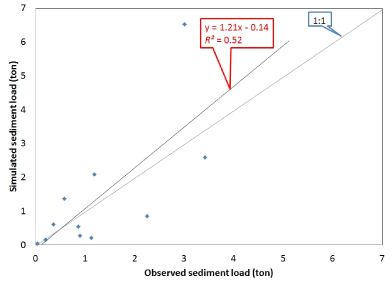
Validation of suspended sediment loads: Table 11 shows the observed and simulated suspended sediment loads by storm events. Over the validation time period (January 1, 1999 to December 31, 1999) there were 11 rainfall events with observed suspended sediment data. The RE values ranged from -81.39% to 134.11%, smaller than the ones found in the calibration period. The average relative error for the simulated suspended sediment loads was 8.78%, smaller than the one computed in the calibration period. The range and average of observed sediment loads were close in the calibration and validation periods. Four out of the 11 events were into the +/-50% RE range. The coefficient of determination (R²) value for the validation period was 0.52, larger than the one computed for the calibration period (R²=0.39). The Nash- Sutcliffe (NS) value of -0.38 indicated that the mean observed value was a better predictor than the simulated value, which indicated unacceptable performance. The RMSE for the validation period was 4.42 ton, almost three times higher than the value computed in the calibration period (RMSE=1.42). The average simulated suspended sediment load values were approximately 9.16% higher than the observed data. Calibration and validation periods showed a tendency of over predict sediment loads by HSPF. Overall, the validation period showed slightly better results than the results in the calibration period.

Figure 6 shows observed and simulated suspended sediment loads by storm events. Validation results were widely scattered around the 1:1 line. Scatter was high and correlation was fair (R²=0.52). The ration between under predicted and over predicted events was almost even (6/5). The slope and intercept values of linear regression equations in the calibration and evaluation periods were close.

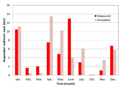
Seasonal and long-term sediment load performance: When analyzing the total suspended sediment loads by month, the overall simulated suspended sediment load values were higher than the observed ones by approximately 9.97%. Monthly RE values ranged from -76.45% to 220.50% with an average value of 37.79% (Table 12). The R² and NS goodness-of-fit values were 0.35 and 0.01, respectively, indicating poor model performance. With the elimination of the extreme events observed in June, the R² and NS statistics significantly increased to fair values of 0.70 and 0.11, respectively. The RMSE figures with and without June data were 12.84 ton and 9.25 ton, respectively. Analysis of runoff values using June events were under predicted by the model by 21.20%. This lack of runoff can partially explain the low values of sediment loads computed by HSPF. In addition, four out six events used in June evaluation were collected in less than 24 hours in 1997. This could suggest that rainfall, water level, and water sample data could present high uncertainty. In addition, it can be seen that some soil disturbances occurred in the month of June. From the field report published by Yuan [15], it was found that herbicide was applied early on June every year. However, no additional soil detachment values were input into the model. In general, low differences and fair correlations demonstrated that the HSPF model did a good performance in modelling suspended sediment loads in the Deep Hollow watershed for long-term monthly intervals.

Figure 7 shows the total suspended sediment loads by month. The HSPF model tracked well the monthly variability of suspended sediment loads from the Deep Hollow agricultural drainage area. All values appear good and reasonable except for the observed suspended sediment for the month of June. It is clear how the June events impacted the goodness-of-fit values. The observed suspended sediment value in June is unreasonably high. Land management actions could be the cause for this increased value but none were recorded. The model was able to simulate close values in the wet season (December and January) and dry season (October). This show the robustness of the HSPF model in simulating seasonal suspended sediment loads in an agricultural farm in the Mississippi Delta region.

Runoff and sediment yield: Table 13 shows the simulated versus the observed values of the previously calculated runoff and the sediment yields in the Deep Hollow watershed. Runoff discrepancies were lower than sediment differences. In this study, simulated annual runoff discrepancies ranged from -18.67% to 1.25% and simulated annual sediment load differences oscillated between -50.34% and 57.84%. Annual AnnAGNPS discrepancies reported by Yuan [14] ranged from -8% to 26% for runoff and -66% to 52% for sediment yield. On average, HSPF model results tended to under predict annual runoff by 10.62% and over predict annual sediment yields by 5.67%. The AnnAGNPS application [14] tended to under predict runoff (15%) and slightly over predict sediment yield (4%).

Phosphorus processes

Calibration of phosphorus loads: Soil initial phosphorus values used in this research are shown in Table 14. The initial organic phosphorus value in surface layer was extracted from [22]. The remaining initial phosphorus storages by layer were assumed. Annual phosphate plant uptake values were found through literature review. Cotton phosphate uptake was set at 2.77 kg/ha [15]. Soybean phosphate uptake was set at 14.42 kg/ha [15]. Winter wheat phosphate uptake was set at 4.49 kg/ha [23]. Monthly fractions of total annual P uptake were developed using data from Liu (2006) for soybean and winter wheat and from Schwab [24] for cotton. The soil layer fraction of monthly uptake rate was developed based on the crop growth stage and the typical depth of crop root. It was assumed that more than 90% of the monthly phosphate uptake came from upper and lower soil layers. The amount of uptake in the groundwater zone was set as zero. Calibrated values of adsorption and desorption of phosphate parameters using the Freundlich method are shown in Table 15.

Table 16 shows the observed and simulated dissolved phosphorus (DP) loads by storm in the calibration period. Twelve out of 19 storm events were into the +/-50% RE range. The model had a tendency of over predict DP loads (14 positive RE values). The R² and NS values were 0.53 and 0.50, respectively. In general, the storm-by-storm HSPF DP load simulation was good with a marked tendency of over predict DP loads.

Table 17 depicts the observed and simulated total phosphorus (TP) loads by storm in the calibration period. Approximately 58% (11 out of 19 events) events were into the +/-50% RE range. Model results did not show any trend (10 negative RE values), but were highly scattered around the 1:1 line. The R² and NS values were 0.60 and 0.04, respectively. All the events simulated in June were under predicted by HSPF. In general, the storm-by-storm HSPF TP load simulation was good with a marked tendency of under predict TP loads in June. TP load discrepancies in June values could be explained by the low sediment load figures simulated by HSPF.

Validation of phosphorus loads: Only four storm events were available with DP and TP data in the validation period (Tables 18 and 19). In general, validation events were lower than those used in the calibration period. HSPF DP load discrepancies ranged from -50.24% to 87.79%. Relative errors between simulated and observed TP values varied from -61.96% to 8.38%. In general, correlations were good for DP and TP loads simulated by HSPF with R² values larger than 0.86 and NS figures larger than 0.30.

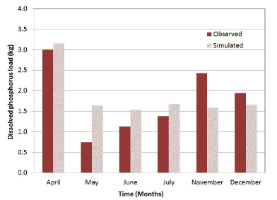
Seasonal and long-term phosphorus load performance: Figure 8 shows simulated and observed monthly DP loadings data from 1997 to 1999. The simulation displays good correspondence with the measured data. The HSPF model simulated the highest monthly DP load (April) very close with a discrepancy around 5%. Generally, simulated and observed long-term monthly correlations were fair (R²=0.50 and NS=0.48). Long-term annual discrepancy was very low (RE=5.82%). The simulation of yearly DP suggested a very good model performance (R²=0.98 and NS=0.94).

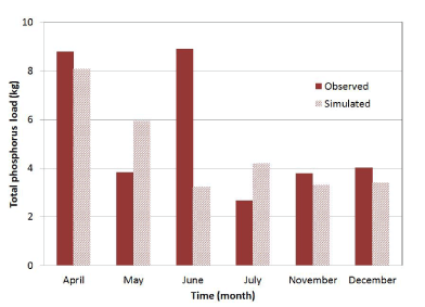
Figure 9 presents simulated and observed monthly TP loadings data from 1997 to 1999. The trend of simulation seems to match the measured data reasonably well, except for large discrepancies in the month of June. This could be partially attributed to the underestimated suspended sediment load by the model in the particular month. The relative low R² (0.13) and NS (-0.05) values indicated a poor simulation of long-term monthly TP simulations. However, if June result is taken out of the analysis, the R² and NS statistics were up to 0.69 and 0.66, respectively, indicating a good model performance. The simulation of yearly TP suggested a good model performance, with R² and NS goodness-of-fit of 0.92 and 0.62, respectively (Table 20).

Discussion

Field data

Table 21 shows monthly observed data used in this study. January, February, March, and October only displayed data of runoff and sediment load. Although some data were collected in August and September, these values were more related to irrigation events rather than storm events. The only linear correspondence was between sediment loads and total phosphorus loads (R²=0.66). This lack of correlation shows that the system is highly manipulated by non-natural conditions. Uncertainty can also rise because not all constituents had the same sample size. This table is useful in analyzing the ration between TP and DP. The observed TP/DP ratio for the study area was 3.0. When June data were taken out of the analysis, a better relation between runoff and sediment load was computed. In addition, the sediment load vs TP load was improved.

Model capabilities and limitations

The accuracy of any environmental model cannot be higher than the accuracy of input data and observed data. The HSPF rainfall-runoff simulation was performed using parameter values related to soil and crop characteristics of the study area. Infiltration rates by soil type were extracted from the USDA SSURGO database. Soil infiltration rates varied from 0.18 mm/h to 2.03 mm/h with a mean value of 0.4 mm/h. HSPF parameters representing rainfall interception by vegetation (INTERCEP), Manning’s roughness factor (NSUR), and lower zone ET (LZETP) were calibrated by month. In this study, monthly parameter variations were important to represent seasonal crop growth and soil moisture variations.

The HSPF model was setup to rainfall data collected every 15 minutes at the site. The observed runoff was computed using a stagedischarge rating curve. Sediment and phosphorus data were collected discretely and sparingly. Malfunctions of the rain gauge and data manipulation could affect HSPF modelling results. In addition, missed observed data and uncertainty in laboratory analysis may affect model evaluation. Finally, uncertainties in input model data (e.g., rainfall, area size, and hydrological response unit discretisation, crop management operations), HSPF algorithms (equations, parameters, and solvers), and evaluation time series (observed runoff , suspended sediments, and dissolved and total phosphorus) may cause the resulting discrepancies between simulated and observed values.

Sediment and phosphorus export processes in agricultural fields are affected by crop management operations. This study used farm records published by Yuan [15]. In the HSPF model, special actions for sediment detachment were coded with planting and harvest dates every year. There is no particle discretisation of HSPF soil erosion values from land surface. Soil particle discretisation is required in HSPF stream processes. In this study, the soil profile was divided into four layers (Table 22). The phosphorus fertilizer was in the form of PO4 for cotton fields. The amount of PO4 fertilizer applied in October 6, 1998 was 72.8 kg/ha. It was assumed that 10% of PO4 reached the surface layer and 90% was incorporated in the upper layer. Soybeans did not receive phosphorus fertilization. Although organic residues were left in the fields as conservation tillage practice, the effects of crop residue on phosphorus concentrations in runoff were not simulated. Irrigation was scheduled in the study area but the model did not simulate it. Runoff and sediment from irrigation could deplete the phosphorus pools in the study area. Atmospheric deposition of phosphorus was not simulated.

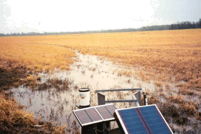
The model did not simulate water detention processes created at the outlet of the study area (Figure 10). Detention processes (flow routing, sediment deposition/scour, nutrient transformations) can be simulated in HSPF using the stream module algorithms (RCHRES).

Table 23 shows monthly simulated data yielded in this study. The simulated TP/DP ratio for the study area was 2.5, a close value compared to the observed one (3.0). The simulated correlation between runoff and sediment load (R²=0.45) was higher than the one computed using observed data (R²=0.12). Simulated DP and TP loads were highly correlated with HSPF sediment load values. Observed sediment loads were highly correlated with observed TP load figures. In general, the model showed similar tendencies among variables as those found in observed time series. This analysis reaffirms that the Deep Hollow drainage area is very complex and the use of process-based models, such as HSPF, is required to find realistic and dynamic answers.

Time scales

This research used data from an intensive field study in an agricultural drainage area between 1996 and 1999 in the Mississippi Delta region [5]. Field data was used to setup and evaluate the HSPF model. In this particular study, climate time series were available or developed every 15 minutes to be input into the HSPF model. The model ran with a 15-minute time step and model results were lumped by storm event. Then, model results were aggregated by month and annual time steps.

Runoff simulation was very good simulated by HSPF across the different time steps (Table 24). Sediment load was poor simulated by storm time steps. However, long-term monthly and annual values were quite good and HSPF reproduced good seasonal sediment processes at the crop farm scale. Simulated dissolved phosphorus (DP) loads were better at long-term time steps than storm-by-storm periods. HSPF total phosphorus (TP) loads were better at simulating long-term periods than storm-by-storm time steps. Generally, seasonal TP load processes modelled by HSPF were good simulated. Additionally, the model simulated a close value of TP/DP ratio measured at the drainage area outlet. In general, the HSPF model is very robust for hydrologic process from storm to long-term time steps.

Sediment export processes from agricultural fields are heavily depended on management operations. The HSPF special actions block is useful in handling farm management operations. This block is developed with specific field operations. In the current study, it was found that storm events in June were significantly under predicted by the model but no field records were available to be inputted into the model. In general, this model evaluation indicates that the HSPF hydrologic, sediment, phosphorus modules are very robust to simulate seasonal and long-term trends in agricultural fields in the Mississippi Delta region.

Summary and Conclusions

The HSPF model is supported by USEPA and USGS agencies since 1980. The model has extensive successful applications around the world mainly evaluating rainfall-runoff processes in large size drainage areas (e.g., larger than 10 km²) with continuous stream flow time series (e.g., average daily data). This research showed results of an assessment of the HSPF hydrology, soil erosion, and phosphorus model at the farm scale in the Mississippi Delta region. The study area is located in the Deep Hollow watershed, Mississippi. The farm size is 11.29 ha with soybeans, cotton, and winter wheat crop rotation. Crop residues were incorporated into soil after harvest. Deep Hollow watershed is in the Mississippi alluvial valley with flat and low infiltration rate soils. In general, the region’s climate is subtropical with hot & humid summers and mild winters. Rainfall, runoff, and concentrations of suspended sediments, dissolved phosphorus and total phosphorus were collected and analyzed by USGS at the outlet of the drainage area from 1996 to 1999. When analyzing the USGS datasets, 69 events were selected to setup and evaluate the HSPF model. Model evaluation consisted in splitting the available data in two different time periods, calibration from 1997 to 1998 and validation in 1999. Runoff processes were evaluated using 45 events for calibration and 24 events for validation. In evaluating sediment export processes, 29 and 11 storm events were utilized in calibration and validation periods, respectively. Phosphorus simulations (dissolved and total) were evaluated using 19 and four storm events in calibration and validation periods, respectively. The HSPF model was setup to evaluate runoff, soil erosion, dissolved & total phosphorus to storm, monthly, and annual time scales.

This study concluded that the HSPF runoff model’s simulations of storm-by-storm, long term monthly and annual intervals were very good. In simulating suspended sediment loads, HSPF performance was poor for storm-by-storm analysis. However, long term monthly, and annual suspended sediment load simulations were tracked fair and good, respectively. Simulations of dissolved phosphorus of storm-bystorm and long term monthly intervals were good. Simulated annual dissolved phosphorus loads correlated very well with observed data. Similarly, HSPF performed good in simulating long term monthly total phosphorus loads and showed very good results in modelling annual total phosphorus loads exported from Deep Hollow drainage area.

We suggest that the simulation conducted in the Deep Hollow drainage area could be used to assess the impact on land use changes, climate variability and soil & nutrient management practices (BMPs) in the future, since hydrology, sediments and phosphorus were evaluated. The study demonstrated that the HSPF model is a capable modelling tool for evaluating runoff, soil erosion, and total phosphorus processes at the farm scale in the Mississippi alluvial valley, mainly for analysis on long term basis (monthly, seasonal, or annual). Results from this study are significant at the scale of this drainage area (11.29 ha), but more study is needed to determine whether processes are accurately predicted.

Overall, HSPF model is a reasonable seasonal and annual predictor of the farm processes for assessing the impacts of different agricultural management practices on runoff, suspended sediment loads, and dissolved & total phosphorus loads. The results of this research would be helpful in providing initial parameter values and guidelines for future applications of HSPF in similar agricultural drainage areas in the Mississippi Delta region.

Acknowledgement

This research was performed with funding from the Mississippi Department of Marine Resources project: “Watershed Assessment Tools: MS Delta Evaluation.” The authors appreciate the comments, pictures, rainfall time series, and water data facilitated by Mr. Richard Rebich from the USGS Mississippi Water Science Center. We like to thank Dr. Ronald Bingner from the USDA National Sedimentation Laboratory for supplying GIS data and relevant information of the study area. Special thanks to Germania Salazar, Matt Moran, and Alina Young, former MSU Civil and Environmental Engineering graduate students funded by this project, for helping in model setup and time series analysis. The support provided to the first author by the USDA-NIFA Evans Allen project: “Sustainable Agriculture and the Environment” is recognized.

References

- Bicknell BR, Imnoff JC Jr, Jobes TH, Donigian AS (2001) Hydrological Simulation Program - FORTRAN (HSPF) version 12, User’s Manual. Prepared for AQUA TERRA Consultants Mountain View, California, in cooperation with Water Resources Discipline U.S. Geological Survey Reston, Virginia , USA.
- Neitsch SL, Arnold JG, Kiniry JR, Williams JR (2011) Soil and Water Assessment Tool: Theoretical Documentation Version 2009. Texas Water Resources Institute technical Report No. 406. Texas A&M University System, College Station, Texas, USA.
- Gassma PW, Williams JR, Wang X, Saleh A, Osei E, et al. (2009) The Agricultural Environmental Extender (APEX) Model: An Emerging Tool for Landscape and Watershed Environmental Analyses. Technical Report 09-TR 49. Center for Agricultural and Rural Development, Iowa State University, Ames, Iowa, USA.
- Bingner RL, Theurer FD, Yuan Y (2011) AnnAGNPS Technical Processes: Documentation Version 5.2. USDA-ARS, National Sedimentation Laboratory, UK.
- Rebich RA, Knight S (2001) The Mississippi Delta Management Systems Evaluation Areas Project, 1995-99. Information Bulletin 377, Mississippi Agricultural & Forestry Experiment Station, USA.
- Donigian, A.S, Bicknell BR, Imhoff JC (1995) Hydrological Simulation Program - FORTRAN (HSPF). Chapter 12. In: Computer Models of Watershed Hydrology. V.P. Singh (ed). Water Resources Publications. Littleton, CO. pp. 395-442.
- U.S. Environmental Protection Agency-USEPA (2012) Better Assessment Science Integrating Point and Nonpoint Sources (BASINS).
- Linsley RK, Kohler MA, Paulhus JL (1988) Hydrology for Engineers. McGraw-Hill. University of Michigan, USA.
- Negev M (1967) A Sediment Model on a Digital Computer. Technical Report 76. Department of Civil Engineering, Stanford University, California, USA.
- Meyer LD, Wischmeier WH (1969) Mathematical Simulation of the Process of Soil Erosion by Water. Transactions of the ASE 12: 754-758.
- Onstad CA, Foster GR (1975) Erosion Modeling on a Watershed. Transactions of the ASE 18: 288-292.
- Wischmeier WH, Smith DD (1965) Predicting Rainfall-Erosion-Losses from Cropland East of the Rocky Mountains: A Guide for Selection of Practices for Soil and Water Conservation. U.S Department of Agricultural, Washington D.C, USA.
- Moriasi DN, Arnold JG, Van Liew MW, Bingner RL, Harmel RD, et al. (2007) Model Evaluation Guidelines for Systematic Quantification of Accuracy in Watershed Simulations. Transactions of the ASABE 50: 885-900.
- Yuan Y, Bingner RL, Rebich RA (2001) Evaluation of AnnAGNPS on Mississippi Delta MSEA Watersheds. Transactions of the ASABE 44: 1183-1190.
- Yuan, Y, R.L Bingner (2002) Assessment of Best Management Practices for Water Quality Improvement for the Deep Hollow Watershed in Mississippi Delta MSEA Project Using AGNPS. US Department of Agriculture, Agricultural Research Service, National Sedimentation Laboratory, Oxford, Mississippi, USA.
- Hamon WR (1963) Computation of Direct Runoff Amounts from Storm Rainfall. Int Assoc Sci Hydrol Pub 63: 52-62.
- U.S. Department of Agricultural, Natural Resources Conservation Service (USDA-NRCS). 2012. Soil Survey Geographic (SSURGO), USA.
- Bergman MJ, Green W, Donnangelo LJ (2002) Calibration of Storm Loads in the South Prong Watershed, Florida, Using BASINS/HSPF. J American Water Resour Assoc 38: 1423-1436.
- Duda PB, Hummel PR, Donigian Jr AS, Imhoff JC (2012) BASINS/HSPF: Model Use, Calibration, and Validation. Transaction of the ASABE 55: 1523-1547.
- U.S. Environmental Protection Agency-USEPA (2006) BASINS Technical Note 8: Sediment Parameter and Calibration Guidance for HSPF. U.S. Environmental Protection Agency, Office of Water, USA.
- Haan CT, Barfield BJ, Hayes JC (1994) Design Hydrology and Sedimentology for Small Catchments. Academic Press, USA.
- Yuan Y, Locke MA, Gaston LA (2009) Tillage Effects on Soil Properties and Spatial Variability in Two Mississippi Delta Watersheds. Soil Science. 174: 385-394.
- Liu Z (2006) Effective Modeling of Agricultural Practices within Large-Scale Hydrologic and Water Quality Simulations. Mississippi State University Department of Plant and Soil Sciences, USA.
- Schwab GJ, Mullins GL, Burmester CH (2000) Growth and Nutrient Uptake by Cotton Roots under Field Conditions. Comm Soil Sci Plant Anal 31: 149-164.