
Quantitative radiology: automated measurement of polyp volume in computed tomography colonography using Hessian matrix-based shape extraction and volume growing
Introduction
Colorectal cancer is the second leading cause of cancer deaths in the U.S. (1). Computed tomography colonography (CTC), also known as “virtual colonoscopy”, is a technique for detecting colorectal neoplasms by use of a CT scan of the colon. CTC provides an option for a colorectal cancer examination that is less uncomfortable (2,3), less invasive, and less costly (4) than for optical colonoscopy (OC) (We use the term, OC instead of colonoscopy to distinguish it from virtual colonoscopy). Evidence supports CTC as a sensitive and specific method for detection of polyps (5-11). Accordingly, several national societies including the American Cancer Society have endorsed CTC as an option for colorectal cancer screening of average risk, asymptomatic patients (12).
In CTC screening for the detection of polyps, polyp size plays an especially important role in determining malignant potential and the need for intervention (5,6,11,13). The size is the most important single feature for such diagnosis. Current measurement of the single longest linear dimension of a polyp, however, is subjective and has variations among radiologists. As evidence of the variability of such manual linear measurement of polyps at CTC, studies reported inter-observer 95% limits of agreement span ranged from 2.5 to 3.2 mm (14,15). Volume measurement could be more clinically informative than longest linear dimension. However, manual measurement of polyp volumes at CTC suffers from problems of labor intensity and subjectivity. As a medical sign frequently occurring in the population, a consistent and efficient volume metric for polyps at CTC is especially important for informing clinical decisions.
Researchers have studied polyp volume measurement at CTC. Taylor et al. (15) compared manual linear measurement and automated polyp measurement with actual measurement of colectomy specimen of 20 polyps from a patient. They used automated polyp measurement software embedded in developmental CTC viewing software (Colon CAR 1.3; Medicsight). The software requires users to provide seed points opposite each other at the perceived junction between the polyp and the colonic wall. Jeong et al. (14) compared manual linear measurement and automated polyp volume measurement with OC polyp size measurement. They used automated polyp measurement software embedded in a commercial CTC viewing workstation (Extended Brilliance workspace version 3.0; virtual colonoscopy, Cleveland, OH, USA). Dijkers et al. (16) developed an automated segmentation method for polyps based on surface evolution from a seed patch under geometric criteria with surface normal. They tested their method with polyp phantoms. Yao et al. (17) developed an automated method for segmenting polyps based on a combination of knowledge-guided intensity adjustment, fuzzy c-mean clustering, and deformable models.
Our purpose in this study was to develop a 3D automated scheme for measuring polyp volume at CTC based on Hessian matrix-based shape extraction and volume growing. We evaluated its accuracy and efficiency relative to “gold-standard” volumes determined by manual segmentation.
Materials and methods
The Institutional Review Board (IRB) approved this retrospective study. Informed consent for use of cases in this study was waived by the IRB because patient data was de-identified. This study complied with the Health Insurance Portability and Accountability Act, met all standards for good clinical research according to the NIH’s and local IRB’s guidelines.
3D automated scheme for measuring polyp volume
We developed a fully automated scheme for measuring polyp volume at CTC. Our scheme consisted of a computer-aided detection (CADe) scheme for polyps (18-24) and a 3D computerized scheme for segmenting polyps to measure their volumes. Recent advancement in CADe studies can be found in a review paper (25). A major advantage of polyp volume measurement combined with CADe of polyps is that radiologists can obtain the volumes for computer-detected polyps immediately. Technical details of our CADe scheme have been described in refs. (26) and (27), and we do not describe the technical details, because CADe is not the focus of this paper but automated polyp volume measurement. Our CADe scheme first segmented the colon in CTC images based on anatomy-based extraction and colon-based analysis. Once the colon was segmented, it detected polyps based on morphologic features that characterize polyps. Our automated polyp segmentation followed for measurement of volumes of the polyps detected by our CADe. Note that a radiologist can always obtain the volume of a polyp that he/she identifies (i.e., one that our CADe does not detect) by specifying its location.
Our automated measurement scheme for polyp volume consisted of segmentation of colon wall, extraction of a highly polyp-like seed region based on the Hessian matrix, a 3D volume growing technique under the minimum surface expansion criterion for segmentation of polyps, and sub-voxel refinement and surface smoothing for obtaining a smooth polyp surface, as shown in Figure 1A. More detailed steps of our automated measurement scheme are given in Figure 1B. To confine polyp segmentation to colon wall, we first segmented the colon wall with uniform thickness by using anatomic knowledge-based segmentation (28). The anatomy-based segmentation consisted of the following steps. The volume outside the body was segmented based on CT value thresholding followed by a 3D connectivity test (29,30); and the resulting volume is called an “air mask” (Figure 2) (see Figure 2F for an illustration). Bone structures that correspond to the spine, pelvis, and parts of the ribs in the original CTC volume were segmented in the same manner. The 3D gradient of CT values was calculated at each voxel that does not belong to the volume defined by the air mask or the segmented bone structure. Those voxels that have gradient and CT values greater than predefined threshold values were retained. A connected component labeling (29,30) was applied to the retained volumes. The connected component that has the largest number of voxels was identified as the colon wall and called a “colon-wall mask” (The “colon-wall mask” is used for masking colon walls. In that sense, it should be called as a non-colon-wall mask, but we call it a colon-wall mask by following the convention in the field) (see Figure 2B for an illustration).


Our seed region detection scheme relied on shape features; we applied a Hessian matrix operator which quantifies the local curvature in the 3D image (31). The principal curvatures at a point describe the maximum and minimum rates that the local surface deviates from a plane. Two feature maps can be derived from the principal curvatures, which together provide a measurement of the local shape and the “degree of the shape” at a point. These are known as shape index and curvedness (18,27,31,32), defined as:
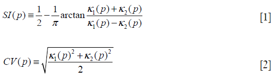
where κ1, κ2 represent the maximum and minimum curvatures, respectively. Figure 2C,D illustrate a shape index map and a curvedness map for a polyp shown in Figure 2A, respectively. We developed a segmentation technique based on region growing (33) to segment the remaining, non-cap-shape region. The two Hessian matrix-based feature maps were used together to extract a cap-shape structure that is typical of a bulbous polyp within the colon-wall mask (illustrated in Figure 2B). To achieve this, first we applied two range threshold operations on each feature map. The first range threshold was narrower than the second. The narrow range threshold operation resulted in a set or sets of very highly polyp-like voxels. The two narrow range threshold images were combined by a Boolean logical multiplication; the two wide range threshold images were similarly combined. We then performed a connectivity analysis based on a connected-component labeling algorithm (29,30) to allow the narrow range threshold region to grow to include any connected wider range threshold voxels. Finally, we applied a mathematical morphologic erosion filter to the thresholded volume to obtain a highly polyp-like seed region (see Figure 2E for an illustration).
For the next step, we developed a segmentation technique based on region growing (33) to segment the remaining, non-cap-shape region. We call this segmentation step 3D volume growing under the minimum surface expansion criterion. First we employed the air mask from the colon-wall segmentation step to distinguish the lumen from non-lumen. Then, we iteratively expanded the highly polyp-like seed region within the non-lumen for a predetermined number of iterations, k, while tracking the volume. Finally, we found the volume in which the surface expansion rate was the minimum as a segmented polyp volume (see Figure 2G for an illustration): the minimum volume expansion point occurs at the x-th iterative expansion when,

where W is the set of expanded voxels.
Finally, to obtain a smooth polyp surface, we applied a 3D sub-voxel refinement technique to the polyp surface in images. First, we resampled the images to obtain higher resolution images with a resampling factor of X, i.e., one original voxel is converted to X3 voxels in the resampled images. Next, we applied a smoothing filter to the resampled surface of the polyp (see Figure 2H for an illustration). Finally, we calculate the volume with accounting for the resampling factor.
CTC database
Our database consisted of 30 polyp views (15 polyps) in CTC scans from 13 patients; these were obtained from a previous multicenter clinical trial in which 15 medical institutions participated nationwide (34). This multicenter trial included air-contrast barium enema, same-day CTC and colonoscopy, and segmental unblinding for each subject, followed by robust reconciliation of all lesions utilizing the data from all three imaging examinations (thereby assuring accuracy of the reported consensus colon findings). Table 1 summarizes the characteristics of our database. Six hundred fourteen high-risk subjects participating in the original trial were scanned in both supine and prone positions with a multi-detector-row CT system with collimations of 1.0-2.5 mm and reconstruction intervals of 1.0-2.5 mm. Each CT slice had a spatial resolution of 0.5-0.7 mm/pixel. A radiologist experienced in CTC (>1,000 cases read) reviewed CTC cases carefully and determined the locations of polyps with reference to colonoscopy reports. Polyp morphology in our database includes pedunculated polyps and sessile polyps. Polyp sizes measured in OC ranged from 6-18 mm (average: 10.4 mm). Note that optical-colonoscopy-measured polyp sizes may not be accurate because it was done by visual assessment of size in linear measurement. That motivated CTC measurement of polyp volume.

Full table
Evaluation
To establish “gold-standard” polyp volumes, an abdominal radiologist outlined polyps in each axial CT image on a viewing workstation and calculated volumes by summation of the volumes obtained by multiplying the areas of the manually outlined regions in each slice by the reconstruction interval [We do not use the term, slice thickness or collimation, because they do not always equal a reconstruction interval (or distance between slices)]. High-quality magnification enabled drawing precise contours. The measurement study was repeated 3 times at least 1 week apart to minimize a memory effect bias. We used the mean volume of the three studies as “gold standard”. The prone and supine volumes were averaged for polyp-based analysis.
We compared computer-estimated volumes obtained by using our automated measurement scheme with the “gold-standard” manual volumes. To evaluate the agreement between the two volumetrics, we used the intra-class correlation analysis (35,36) and the Bland-Altman analysis (37). Statistical significance was analyzed by using the F-test.
Results
Polyp volumes obtained by using our scheme
Figure 3 illustrates three manual outlines drawn by an abdominal radiologist in three measurement studies for a polyp. The intra-observer variation in polyp outlining is larger for the edges of the polyp (A) and (C), compared to the middle of the polyp (B). We used an average outline over three outlines as “gold standard.” We applied our automated measurement scheme to our database containing 30 polyp views from 15 polyps in 13 patients. Resulting images from each step in our scheme is illustrated in Figure 2. Figure 4 illustrates the result of automated polyp segmentation for supine and prone views of a polyp. There was a difference (0.06 cc) in manual volumes for supine and prone views. The average computer volume of 0.18 cc is equal to the average “gold-standard” manual volume of 0.18 cc. Relationships between supine and prone volumes for same polyps are shown in Figure 5. Both manual and computer volumes for supine and prone views agree moderately. Figure 6 illustrates the computer contours obtained by using our automated scheme and the corresponding “gold-standard” manual contours. Although they show some difference, most of differences are within one pixel. Figure 7 shows a relationship between “gold-standard” manual volumes and computer volumes in the polyp-based analysis. The two volumes agree well for smaller polyps.


Statistical analysis
Our scheme yielded a mean polyp volume of 0.38 cc (range, 0.15-1.24 cc), whereas the mean “gold-standard” manual volume was 0.40 cc (range, 0.15-1.08 cc), as shown in Table 2. Table 3 summarizes the results of intra-class correlation analysis for supine vs. prone volumes and computer vs. manual volumes. The “gold-standard” manual and computer volumetrics reached excellent agreement [intraclass correlation coefficient (ICC) =0.80], with no statistically significant difference [P (F≤f) =0.42], as shown in Table 3. The Bland-Altman plot of computer and manual polyp volumes is shown in Figure 8. The two volumes disagree for larger polyps, although the number of samples of large polyps is very small. Table 4 shows a bias and 95% limits of agreement in the Bland-Altman analysis. The 95% limits of agreement span was relatively large (0.71 cc).

Full table

Full table


Full table
Discussion
Although we achieved an excellent agreement between computer-estimated polyp volumes and “gold-standard” manual polyp volumes (ICC =0.80), there is still difference with “gold-standard” volumes especially for larger polyps. To determine the boundary between the colonic wall and a polyp attaching to it is challenging, because the same soft-tissue of similar or same density constitutes the colonic wall and the polyp; thus, there is no distinct boundary between them in most cases. To our knowledge, there is no consensus as to how the boundary between them should be determined in the radiology community. To address this issue, the radiology community would need to develop robust criteria to determine the boundary and build a consensus.
There are a few parameters to adjust in our scheme. We adjusted these parameters based on the visual judgment with cases in an independent database (completely different from the database we used in this study) without reference to manual segmentation. Thus, the parameters were not optimized. In the future, we will need to optimize the parameters by using a larger number of cases with reference to “gold-standard” manual segmentation. On the other hand, because the parameter adjustment was done independently, our scheme is likely to achieve the same or similar level of performance that we obtained in this study when we apply our scheme to a different database.
We cannot compare our scheme with other schemes in the literature directly because the cases were different for each study, but we discuss similarities and differences of our scheme with these schemes. Jeong et al. (14) used automated polyp measurement software embedded in a commercial CTC viewing workstation (Extended Brilliance workspace version 3.0; virtual colonoscopy, Cleveland, OH, USA) in their study. They did not mention any technical details of the automated software, because they could not know such information due to commercial software. They did not perform volume comparisons, because their study purpose was to compare measurements at CTC with OC measurement. Taylor et al. (15) used automated polyp measurement software embedded in developmental CTC viewing software (Colon CAR 1.3; Medicsight) in their study. They mentioned the automated software was based on fuzzy logic-based region growing, but they did not provide any other technical details. The measurement software is semi-automated, because it requires users to provide two seed points opposite each other at the perceived junction between the polyp and the colonic wall. As we discussed earlier, determining the junction between the polyp and the colonic wall is challenging for fully automated measurement schemes such as ours. Dijkers et al. (16) developed an automatic polyp segmentation method based on surface evolution from a seed patch under geometric criteria with surface normal. They tested their method with polyp phantoms, but they did not test with actual polyps from patients. Their method requires no user input. Yao et al. (17) developed an automated method for segmenting polyps based on fuzzy c-mean clustering and deformable models. Their scheme requires no user input; thus, it is fully automated. Our scheme is also a fully automated polyp volume measurement scheme that requires no user input. In our scheme, Hessian-feature-based extraction of a highly polyp-like seed region, 3D volume-growing-based segmentation of polyps under the minimum surface expansion criterion, and sub-voxel refinement were developed for accurately determining polyp volume. In particular, detection of a highly polyp-like seed region improved the robustness of volume growing substantially. None of the above conventional schemes used Hessian-based seed region identification or 3D volume growing under the minimum surface expansion criterion.
Our database used in this study does not contain “flat” lesions (38,39), but only polypoid and sessile lesions. Flat lesions may be defined as the height of a lesion less than 3 mm or the height less than one-half the width as seen on 2D views or a long axis as seen on 3D views. We will need to test our automated polyp volume measurement scheme with flat lesions for complete testing. To our knowledge, there is no study to test a polyp size measurement scheme on flat lesions in literature.
Some practices and tasks in radiology as well as other clinical medicine areas have been qualitative and subjective. We define quantitative radiology as efforts to make practices and tasks in radiology more quantitate, objective, and evidence-based. We believe that quantitative radiology is one major trend and direction that radiology would go. We have developed automated liver volume measurement schemes in CT (40,41) and MRI (42) as a mean for quantitative liver volume assessment in quantitative radiology. Our automated liver volumetry schemes in CT and MRI agreed with “gold-standard” manual volumetry excellently. In this study, we developed an automated polyp volume measurement scheme in CTC. Quantitative liver volumetry can be considered as an organ volumetry, whereas quantitative polyp volumetry can be considered as a lesion volumetry. We plan to expand quantitative radiology areas to include other major organs and lesions in addition to quantitative liver and polyp volumetry.
Conclusions
We developed an automated scheme for measuring polyp volume at CTC. Our automated polyp volumetrics agreed excellently with “gold standard” manual volumetrics (ICC =0.80 with no statistical significant difference). Our automated scheme can efficiently provide accurate polyp volumes for radiologists; thus, it would help radiologists improve the accuracy and efficiency of polyp volume measurements at CTC.
Acknowledgements
Computer-aided diagnosis and machine-learning technologies developed at the University of Chicago have been licensed to companies including R2 Technology (Hologic), Riverain Medical (Riverain Technologies), AlgoMedica, Median Technologies, Mitsubishi Space Software, General Electric, and Toshiba. Some implementations used ITK.
Funding: This work was partially supported by Grant Number R01CA120549 from the National Cancer Institute/National Institutes of Health.
Footnote
Conflicts of Interest: The authors have no conflicts of interest to declare.
References
- American Cancer Society. Colorectal Cancer Facts & Figures 2014-2016. Atlanta: American Cancer Society, 2014.
- Svensson MH, Svensson E, Lasson A, Hellström M. Patient acceptance of CT colonography and conventional colonoscopy: prospective comparative study in patients with or suspected of having colorectal disease. Radiology 2002;222:337-45. [PubMed]
- van Gelder RE, Birnie E, Florie J, Schutter MP, Bartelsman JF, Snel P, Laméris JS, Bonsel GJ, Stoker J. CT colonography and colonoscopy: assessment of patient preference in a 5-week follow-up study. Radiology 2004;233:328-37. [PubMed]
- Pickhardt PJ, Hassan C, Laghi A, Zullo A, Kim DH, Morini S. Cost-effectiveness of colorectal cancer screening with computed tomography colonography: the impact of not reporting diminutive lesions. Cancer 2007;109:2213-21. [PubMed]
- Pickhardt PJ, Choi JR, Hwang I, Butler JA, Puckett ML, Hildebrandt HA, Wong RK, Nugent PA, Mysliwiec PA, Schindler WR. Computed tomographic virtual colonoscopy to screen for colorectal neoplasia in asymptomatic adults. N Engl J Med 2003;349:2191-200. [PubMed]
- Kim DH, Pickhardt PJ, Taylor AJ, Leung WK, Winter TC, Hinshaw JL, Gopal DV, Reichelderfer M, Hsu RH, Pfau PR. CT colonography versus colonoscopy for the detection of advanced neoplasia. N Engl J Med 2007;357:1403-12. [PubMed]
- Johnson CD, Toledano AY, Herman BA, Dachman AH, McFarland EG, Barish MA, Brink JA, Ernst RD, Fletcher JG, Halvorsen RA Jr, Hara AK, Hopper KD, Koehler RE, Lu DS, Macari M, Maccarty RL, Miller FH, Morrin M, Paulson EK, Yee J, Zalis M. American College of Radiology Imaging Network A6656. Computerized tomographic colonography: performance evaluation in a retrospective multicenter setting. Gastroenterology 2003;125:688-95. [PubMed]
- Fenlon HM, Nunes DP, Schroy PC 3rd, Barish MA, Clarke PD, Ferrucci JT. A comparison of virtual and conventional colonoscopy for the detection of colorectal polyps. N Engl J Med 1999;341:1496-503. [PubMed]
- Yee J, Akerkar GA, Hung RK, Steinauer-Gebauer AM, Wall SD, McQuaid KR. Colorectal neoplasia: performance characteristics of CT colonography for detection in 300 patients. Radiology 2001;219:685-92. [PubMed]
- Johnson CD, Herman BA, Chen MH, Toledano AY, Heiken JP, Dachman AH, Kuo MD, Menias CO, Siewert B, Cheema JI, Obregon R, Fidler JL, Zimmerman P, Horton KM, Coakley KJ, Iyer RB, Hara AK, Halvorsen RA Jr, Casola G, Yee J, Blevins M, Burgart LJ, Limburg PJ, Gatsonis CA. The National CT Colonography Trial: assessment of accuracy in participants 65 years of age and older. Radiology 2012;263:401-8. [PubMed]
- Johnson CD, Chen MH, Toledano AY, Heiken JP, Dachman A, Kuo MD, Menias CO, Siewert B, Cheema JI, Obregon RG, Fidler JL, Zimmerman P, Horton KM, Coakley K, Iyer RB, Hara AK, Halvorsen RA Jr, Casola G, Yee J, Herman BA, Burgart LJ, Limburg PJ. Accuracy of CT colonography for detection of large adenomas and cancers. N Engl J Med 2008;359:1207-17. [PubMed]
- Levin B, Lieberman DA, McFarland B, Smith RA, Brooks D, Andrews KS, Dash C, Giardiello FM, Glick S, Levin TR, Pickhardt P, Rex DK, Thorson A, Winawer SJ; American Cancer Society Colorectal Cancer Advisory Group; US Multi-Society Task Force; American College of Radiology Colon Cancer Committee. Screening and surveillance for the early detection of colorectal cancer and adenomatous polyps, 2008: a joint guideline from the American Cancer Society, the US Multi-Society Task Force on Colorectal Cancer, and the American College of Radiology. CA Cancer J Clin 2008;58:130-60. [PubMed]
- Macari M, Bini EJ. CT colonography: where have we been and where are we going? Radiology 2005;237:819-33. [PubMed]
- Jeong JY, Kim MJ, Kim SS. Manual and automated polyp measurement comparison of CT colonography with optical colonoscopy. Acad Radiol 2008;15:231-9. [PubMed]
- Taylor SA, Slater A, Halligan S, Honeyfield L, Roddie ME, Demeshski J, Amin H, Burling D. CT colonography: automated measurement of colonic polyps compared with manual techniques--human in vitro study. Radiology 2007;242:120-8. [PubMed]
- Dijkers JJ, van Wijk C, Vos FM, Florie J, Nio YC, Venema HW, Truyen R, van Vliet LJ. Segmentation and size measurement of polyps in CT colonography. Med Image Comput Comput Assist Interv 2005;8:712-9. [PubMed]
- Yao J, Miller M, Franaszek M, Summers RM. Colonic polyp segmentation in CT colonography-based on fuzzy clustering and deformable models. IEEE Trans Med Imaging 2004;23:1344-52. [PubMed]
- Yoshida H, Näppi J. Three-dimensional computer-aided diagnosis scheme for detection of colonic polyps. IEEE Trans Med Imaging 2001;20:1261-74. [PubMed]
- Suzuki K, Rockey DC, Dachman AH. CT colonography: advanced computer-aided detection scheme utilizing MTANNs for detection of "missed" polyps in a multicenter clinical trial. Med Phys 2010;37:12-21. [PubMed]
- Suzuki K, Yoshida H, Näppi J, Armato SG 3rd, Dachman AH. Mixture of expert 3D massive-training ANNs for reduction of multiple types of false positives in CAD for detection of polyps in CT colonography. Med Phys 2008;35:694-703. [PubMed]
- Suzuki K, Yoshida H, Näppi J, Dachman AH. Massive-training artificial neural network (MTANN) for reduction of false positives in computer-aided detection of polyps: Suppression of rectal tubes. Med Phys 2006;33:3814-24. [PubMed]
- Xu JW, Suzuki K. Max-AUC feature selection in computer-aided detection of polyps in CT colonography. IEEE J Biomed Health Inform 2014;18:585-93. [PubMed]
- Xu JW, Suzuki K. Massive-training support vector regression and Gaussian process for false-positive reduction in computer-aided detection of polyps in CT colonography. Med Phys 2011;38:1888-902. [PubMed]
- Suzuki K, Zhang J, Xu J. Massive-training artificial neural network coupled with Laplacian-eigenfunction-based dimensionality reduction for computer-aided detection of polyps in CT colonography. IEEE Trans Med Imaging 2010;29:1907-17. [PubMed]
- Suzuki K. A review of computer-aided diagnosis in thoracic and colonic imaging. Quant Imaging Med Surg 2012;2:163-76. [PubMed]
- Näppi J, Dachman AH, MacEneaney P, Yoshida H. Automated knowledge-guided segmentation of colonic walls for computerized detection of polyps in CT colonography. J Comput Assist Tomogr 2002;26:493-504. [PubMed]
- Yoshida H, Masutani Y, MacEneaney P, Rubin DT, Dachman AH. Computerized detection of colonic polyps at CT colonography on the basis of volumetric features: pilot study. Radiology 2002;222:327-36. [PubMed]
- Masutani Y, Yoshida H, MacEneaney PM, Dachman AH. Automated segmentation of colonic walls for computerized detection of polyps in CT colonography. J Comput Assist Tomogr 2001;25:629-38. [PubMed]
- He L, Chao Y, Suzuki K, Wu K. Fast connected-component labeling. Pattern Recognition 2009;42:1977-87.
- Suzuki K, Horiba I, Sugie N. Linear-time connected-component labeling based on sequential local operations. Computer Vision and Image Understanding 2003;89:1-23.
- Dorai C, Jain A. COSMOS-A representation scheme for 3D free-form objects. IEEE Transactions on Pattern Analysis and Machine Intelligence 1997;19:1115-30.
- Koenderink JJ, van Doorn AJ. Surface shape and curvature scales. Image and Vision Computing 1992;10:557-64.
- Shapiro LG, Stockman GC. Computer Vision. New Jersey: Prentice-Hall, 2001:279-325.
- Rockey DC, Paulson E, Niedzwiecki D, Davis W, Bosworth HB, Sanders L, Yee J, Henderson J, Hatten P, Burdick S, Sanyal A, Rubin DT, Sterling M, Akerkar G, Bhutani MS, Binmoeller K, Garvie J, Bini EJ, McQuaid K, Foster WL, Thompson WM, Dachman A, Halvorsen R. Analysis of air contrast barium enema, computed tomographic colonography, and colonoscopy: prospective comparison. Lancet 2005;365:305-11. [PubMed]
- Portney LG, Watkins MP. Foundations of clinical research: applications to practice. Norwalk, Conn.: Appleton & Lange, 1993:509-16.
- Shrout PE, Fleiss JL. Intraclass correlations: uses in assessing rater reliability. Psychol Bull 1979;86:420-8. [PubMed]
- Bland JM, Altman DG. Statistical methods for assessing agreement between two methods of clinical measurement. Lancet 1986;1:307-10. [PubMed]
- Lostumbo A, Suzuki K, Dachman AH. Flat lesions in CT colonography. Abdom Imaging 2010;35:578-83. [PubMed]
- Lostumbo A, Wanamaker C, Tsai J, Suzuki K, Dachman AH. Comparison of 2D and 3D views for evaluation of flat lesions in CT colonography. Acad Radiol 2010;17:39-47. [PubMed]
- Suzuki K, Epstein ML, Kohlbrenner R, Garg S, Hori M, Oto A, Baron RL. Quantitative radiology: automated CT liver volumetry compared with interactive volumetry and manual volumetry. AJR Am J Roentgenol 2011;197:W706-12. [PubMed]
- Suzuki K, Kohlbrenner R, Epstein ML, Obajuluwa AM, Xu J, Hori M. Computer-aided measurement of liver volumes in CT by means of geodesic active contour segmentation coupled with level-set algorithms. Med Phys 2010;37:2159-66. [PubMed]
- Huynh HT, Karademir I, Oto A, Suzuki K. Computerized liver volumetry on MRI by using 3D geodesic active contour segmentation. AJR Am J Roentgenol 2014;202:152-9. [PubMed]

