


Abstract
Ion escape to space through the interaction of solar wind and Mars is an important factor influencing the evolution of the Martian atmosphere. The plasma clouds (explosive bulk plasma escape), considered an important ion escaping channel, have been recently identified by spacecraft observations. However, our knowledge about Martian plasma clouds is lacking. Based on the observations of the Mars Atmosphere and Volatile EvolutioN (MAVEN) spacecraft, we study a sequence of periodic plasma clouds that occurred at low altitudes (∼600 km) on Mars. We find that the heavy ions in these clouds are energy-dispersed and have the same velocity, regardless of species. By tracing such energy-dispersed ions, we find the source of these clouds is located in a low-altitude ionosphere (∼120 km). The average tailward moving flux of ionospheric plasma carried by clouds is on the order of 107 cm−2 s−1, which is one order higher than the average escaping flux for the magnetotail, suggesting explosive ion escape via clouds. Based on the characteristics of clouds, we suggest, similar to the outflow of Earth's cusp, these clouds might be the product of heating due to solar wind precipitation along the open field lines, which were generated by magnetic reconnection between the interplanetary magnetic field and crustal fields that occurred above the source.
Export citation and abstract BibTeX RIS

Original content from this work may be used under the terms of the Creative Commons Attribution 4.0 licence. Any further distribution of this work must maintain attribution to the author(s) and the title of the work, journal citation and DOI.
1. Introduction
Ion escape is a process that occurs through the interaction between the solar wind and the Martian ionosphere. Because of its importance in the evolution of the Martian atmosphere, ion escape has been the subject of intensive research for decades. Several primary plasma escape channels have been proposed in previous studies: (1) pick up ions (Dubinin et al. 2006; Fang et al. 2008, 2010; Dong et al. 2015); (2) plasma sheet outflows (e.g., Modolo et al. 2005; Barabash et al. 2007; Dubinin et al. 2011; Lundin 2011; Brain et al. 2015; Nilsson et al. 2021; Ramstad & Barabash 2021); (3) polar wind ions (e.g., Collinson et al. 2019; Fränz et al. 2010; Xu et al. 2018; Ma et al. 2019); and (4) bulk transport/removal of the plasma via coherent structures (e.g., magnetic flux ropes and plasma clouds) (e.g., Brace et al. 1982; Russell et al. 1982; Harnett 2009; Brain et al. 2010; Hara et al. 2014; Halekas et al. 2016, 2019).
As an important channel of ionospheric plasma escape, plasma clouds have been extensively investigated at both Venus and Mars. Based on the observations of the Pioneer Venus orbiter, Brace et al. (1982) first reported plasma clouds in the Venusian space environment, which are characterized by enhanced electron number density above the ionopause, and found that Venusian plasma clouds were mainly located at the dayside and terminator region. With observations of the Mars Global Surveyor (MGS) spacecraft, Acuña et al. (1998) first reported the possible occurrence of Martian plasma clouds. In the past decades, the Kevin–Helmholtz instability (KHI) at the ionopause was considered as a prior mechanism for generating Martian plasma clouds (e.g., Penz et al. 2004; Pope et al. 2009; Ruhunusiri et al. 2016). Recently, with state-of-the-art instruments and combining with more comprehensive measurements from MAVEN (Jakosky et al. 2015), Halekas et al. (2016) investigated the magnetic and plasma features of plasma clouds occurring at high altitudes (∼3000 km) near the ion composition boundary (ICB). Unlike theories associated with KHI, they suggested that these clouds were generated by a "snowplow effect" that was driven by the magnetic tension force resulting from draped field lines (Russell et al. 1982; DiBraccio et al. 2015). Moreover, the plasma cloud could be regarded as a vital escape channel, contributing approximately 10%–20% in scavenging planetary ions (Halekas et al. 2016).
Nevertheless, our knowledge about Martian plasma clouds is lacking due to the high variability of clouds and the limitations of single-point spacecraft observation. Since heavy ions of clouds must be from the ionosphere, the whole picture about the origin and evolution of clouds should be comprised of the stages when these clouds are found at different altitudes from the ionosphere to the magnetosphere. However, only one case of plasma clouds at a high altitude (∼3000 km) has been comprehensively investigated (Halekas et al. 2016). In this paper, we make a comprehensive study of Martian plasma clouds at a lower altitude (∼600 km) and discuss their generating mechanisms in order to draw a better picture of the evolution of clouds, which will help improve our understanding of loss mechanisms of the Martian atmosphere.
2. Event Analysis
In this study, we adopt magnetic field measurements from the Magnetometer (Connerney et al. 2015), ion data from the Solar Wind Ion Analyzer (SWIA; Halekas et al. 2015a) and the Suprathermal and Thermal Ion Composition (STATIC) instrument (McFadden et al. 2015), and electron data from the Solar Wind Electron Analyzer (SWEA; Mitchell et al. 2016) on board MAVEN. The coordinates utilized here are the Mars Solar Orbital (MSO) coordinates (e.g., Liu et al. 2021), where X points from Mars to the Sun, Y points opposite to Mars' orbital velocity, and Z completes the right-handed system.
From 2019-10-08 23:10 to 2019-10-09 00:00, as illustrated in Figure 1(a), MAVEN moved from the nightside tail region to the dayside region. As indicated by the blue dashed lines in Figures 1(b) and (c), MAVEN crossed the magnetic pileup boundary (MPB) at 23:53, which was identified by a sudden enhancement of magnetic field fluctuation (Figure 1(b)) and hot ions (Figure 1(c)). Interestingly, a set of energy-dispersed events that ions exceeded the escape energy (0.12 eV for H+, 2 eV for O+, 4 eV for  ) were observed during 23:28-23:40, similar to the phenomenon reported by Halekas et al. (2015b). During this interval, MAVEN was located on average at (−0.2, −0.5, 1) Rm (Mars radius, Rm = 3390 km) in MSO coordinates at ∼600 km altitude (gray lines in Figure 1(a)). Within these events, several periodic enhancements of the magnetic field and energy-dispersed ions were simultaneously observed during 23:29-23:36 (as denoted by the vertical dashed lines in Figure 1). This particular observation is reminiscent of the plasma clouds recently reported by Halekas et al. (2016). But unlike those clouds that Halekas et al. (2016) studied, these plasma clouds occurred at a lower altitude (∼600 km). Thus, we refer to them as the low-altitude plasma clouds, whereas the clouds reported by Halekas et al. (2016) are called high-altitude clouds. Other similar energy-dispersed events during 23:36-23:40 are not investigated here due to the absence of accompanying periodic enhancement of the magnetic field.
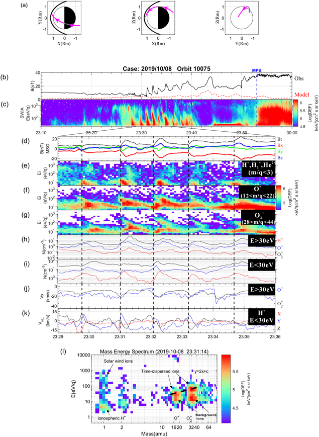
Figure 1. Overview of the periodic plasma cloud event as observed by MAVEN. (a) The location of MAVEN projected in the XY, XZ, and YZ planes in MSO coordinates. The magenta lines with arrows denote the spacecraft's trajectory, and the overlapped gray segments represent the interval (23:29–23:36) when clouds are observed. The black curves represent the position of MPB from the model of Trotignon et al. (2006). (b) The magnetic field strength observed by MAVEN (black solid line) and crustal magnetic field strength (red dashed line) estimated by the model of Gao et al. (2021). (c) The SWIA energy spectrum. (d) The time series of magnetic field in MSO coordinates. (e) Energy spectrum of H+/ . (f) Energy spectrum of O+. (g) Energy spectrum of
  . (h) The number density of high-energy ions (E > 30 eV). (i) The number density of low-energy ions (E < 30 eV). (j) The tailward velocity of high-energy O+ and
  . (k) The perpendicular velocity of low-energy H+. (l) The mass–energy spectrum of ions of the plasma cloud. The vertical dashed lines in each panel denote the start time of each cloud.
Download figure:
Standard image High-resolution image2.1. Features of the Magnetic Field and Ion Distributions
Figures 1(d)–(l) shows the detailed observations of these low-altitude plasma clouds. Similar to the high-altitude clouds, two major magnetic features of the low-altitude plasma clouds were observed: (1) enhanced magnetic field strength, and (2) twisted magnetic field lines characterized by the bipolar variation of the By component (Figure 1(d)).
From STATIC measurements, we find obvious enhancement of the flux of ionospheric O+ (Figure 1(f)) and  (Figure 1(g)) and an increase in ion number density (Figures 1(h), (i)) as well as tailward velocity (Figure 1(j)). These indicate the bulk removal of ionospheric plasma and conform to the definition of plasma clouds (Halekas et al. 2016).
In each cloud, the group of  can be divided into two populations (Figure 1(e)): low-energy plasma (<30 eV) from the ionosphere, and high-energy plasma (30 eV–1 keV) stemmed from solar wind (the two groups of plasma can also be identified in Figure 1(l)). One can see that the flux of low-energy ionospheric
  increased ahead of the magnetic field peaks, while the high-energy solar wind H+ increased around or behind the magnetic field peaks. To some extent, this phenomenon is similar to that of the high-altitude clouds as reported by Halekas et al. (2016), where it was suggested that magnetic field peaks were the interface between the solar wind ions and ionospheric ions (Halekas et al. 2016). However, for low-altitude clouds, as suggested here, solar wind protons coexist with the ionospheric heavy ions (Figures 1(f) and (g)), which does not support the interface interpretation. Instead, we suggest that magnetic reconnection between the IMF and crustal fields might mix solar wind and ionospheric ions (e.g., Harada et al. 2018), which is assessed below.
In addition to the light ions, both the ionospheric heavy ions, O+ and  , have two populations (Figures 1(f) and (g)): energy-dispersed ions (>30 eV) that also occurred in high-altitude clouds (Halekas et al. 2016), and low-energy background ions (<30 eV) that persist during the whole interval and are absent in high-altitude clouds. This difference might result from two aspects: (1) low-altitude plasma clouds were in an earlier developing stage during which background plasma can enter and interact with clouds, while high-altitude clouds, being highly developed, were closed structures (unable to be penetrated by background plasma); (2) they were formed by different mechanisms. Detailed discussion is beyond the scope of this paper. But we note that, in contrast to the equal energy of heavy ions in high-altitude clouds, the tailward velocity of O+ and
  in the low-altitude clouds presented here are approximately equal (Figure 1(j)) and that the energy-dispersed
  has nearly twice the energy of the dispersed O+ (as indicated by the black dashed line in Figure 1(l)), meaning that heavy ions in low-altitude clouds had the same velocity at an instantaneous time.
In addition to the enhanced density of high-energy ionospheric ions due to the arrival of clouds, the density of background ions (Figure 1(i)) increases with increased magnetic field strength, which may indicate the occurrence of compressional signatures (e.g., Futaana et al. 2006; Grigoriev et al. 2006; Collinson et al. 2018; Fowler et al. 2018). Generally, the low-energy ionospheric H+ are magnetized owing to their relatively small gyroradius (energy ∼10 eV, ∣B∣ ∼ 15 nT, the gyroradius ∼30 km), and the electric drift velocity ( ) dominates the perpendicular velocity because of their low energy. Thus, it is helpful to check the compressional structures by the variation of the perpendicular velocity of low-energy H+ (
V
⊥ =
V
− (
V
·
b
)
b
, where
V
is the total velocity and
b
is the unit magnetic field vector). From Figure 1(k), we see that each magnetic field amplification corresponds to +Vy/–Vz, while magnetic field depression coincided with -Vy/+Vz. Combining the location of MAVEN in -Y/+Z side (Figure 1(a)), +Vy/–Vz denotes the inward motion of the magnetic field line, while –Vy/+Vz reflects the outward motion. Thus, enhancements of the magnetic field in low-altitude clouds were associated with transversal variation of plasma flow, which could be caused by compressional structures rather than the shielding current around the interface between solar wind ions and ionospheric ions (Halekas et al. 2016).
) dominates the perpendicular velocity because of their low energy. Thus, it is helpful to check the compressional structures by the variation of the perpendicular velocity of low-energy H+ (
V
⊥ =
V
− (
V
·
b
)
b
, where
V
is the total velocity and
b
is the unit magnetic field vector). From Figure 1(k), we see that each magnetic field amplification corresponds to +Vy/–Vz, while magnetic field depression coincided with -Vy/+Vz. Combining the location of MAVEN in -Y/+Z side (Figure 1(a)), +Vy/–Vz denotes the inward motion of the magnetic field line, while –Vy/+Vz reflects the outward motion. Thus, enhancements of the magnetic field in low-altitude clouds were associated with transversal variation of plasma flow, which could be caused by compressional structures rather than the shielding current around the interface between solar wind ions and ionospheric ions (Halekas et al. 2016).
In this case, the average tailward flux of O+ in these clouds is estimated as ∼2 × 107 cm−2 s−1, and 6 × 107 cm−2 s−1 for  . This flux is approximately an order of magnitude higher than the average observed flux in the magnetotail (on the order of 106 cm−2 s−1) (e.g., Nilsson et al. 2011, 2021; Brain et al. 2015; Inui et al. 2019; Dubinin et al. 2021), which may confirm the explosive bulk removal of plasma via clouds. Moreover, compared with a single cloud, the sequence of periodic clouds contributes to the efficiency of plasma transport and escape more significantly.
2.2. Location of the Source Region
The above analysis shows some similarities and differences between low-altitude and high-altitude clouds. One may ask whether low-altitude clouds could be better explained by the high-altitude cloud scenario presented by Halekas et al. (2016) or by another mechanism.
Generally, the energy-dispersed ions at Mars are a result of the time-of-flight effect: high-energy ions arrive earlier than low-energy ions (e.g., Yau & André 1997; Halekas et al. 2015b), In other words, clouds were initially injected from a source region that is away from the spacecraft location. Thus, one of the most valuable pieces of information that might reveal an explanatory mechanism is the location of the source. The source region and the injection time could be roughly determined by the "1/v-method", which has been successfully applied to Earth (e.g., Keiling et al. 2005). The "1/v-method" can be applied by manually fitting a straight line through a dispersed structure in the 1/v spectrum, the inverse of the slope represents the traveling distance (1/v = (1/L) *t), and the intercept on the 1/v = 0 line denotes the injection time. As displayed in Figures 2(a) and (b), both O+ and  have approximately the same traveling distance and injection time, implying that O+ and
  are produced from the same source. Moreover, traveling distance decreased when the altitude of the spacecraft decreased, suggesting that the source is located below the spacecraft. Assuming that heavy ions move along straight magnetic field lines from a stationary source, the average source location could be determined by the least square method, that is,
  , while (Xs
, Ys
, Zs
) represents the source location, (xi
, yi
, zi
) represents the average location of spacecraft when the ith cloud was observed, and Li
is the traveling distance of the ith cloud (see Figures 2(a)–(b)). Utilizing this method, the estimated location of the source is (−0.075, −0.474, 0.918) Rm in MSO, or (Lon = 73
, while (Xs
, Ys
, Zs
) represents the source location, (xi
, yi
, zi
) represents the average location of spacecraft when the ith cloud was observed, and Li
is the traveling distance of the ith cloud (see Figures 2(a)–(b)). Utilizing this method, the estimated location of the source is (−0.075, −0.474, 0.918) Rm in MSO, or (Lon = 73 5, Lat = 392) with an altitude of ∼120 km in Geocentric coordinates (Figure 2(d)), where the crustal magnetic field should be intense (∼140 nT),as inferred by the latest model of Gao et al. (2021). Thus, our analysis suggests that some processes generating low-altitude clouds might be linked to crustal fields.
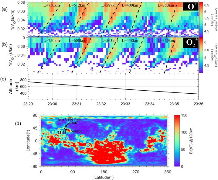
Figure 2. (a) The 1/v spectrum of O+. The black dashed lines are the fitted 1/L. (b) The 1/v spectrum of  . (c) The altitude of MAVEN. (d) The crustal field map from the model of Gao et al. (2021). The black line with an arrow represents the path of MAVEN during 23:29–23:36, while the black pentagram denotes the inferred location of the source region.
Download figure:
Standard image High-resolution image2.3. Magnetic Field Topology
Cloud mechanisms may also be informatively probed by magnetic field topology, which can be diagnosed by electron distribution (e.g., Brain et al. 2007; Xu et al. 2017, 2019). Figure 3(c) shows the pitch angle distribution of electrons with energy 100 eV–300 eV, while Figure 3(d) shows the topology index (0: unknown, 1: closed-to-day (C-D), 2: cross-terminator-closed (C-X), 3: closed-trapped (C-T), 4: closed-voids (C-V), 5: open-to-day (O-D), 6: open-to-night (O-N), 7: draped (DP)), which was obtained by using the technique of Xu et al. (2017, 2019). The closed-to-day type denotes field lines that have both foot points on the dayside ionosphere, which can be identified by photoelectrons traveling in both parallel and antiparallel directions (Figure 3(f)); it typically represents the closed crustal field lines. However, for the open-to-day type, the field line has one of the foot points that ends in the dayside ionosphere, which can be identified by the precipitation of solar wind electrons and an outflow of photoelectrons (Figure 3(e)).
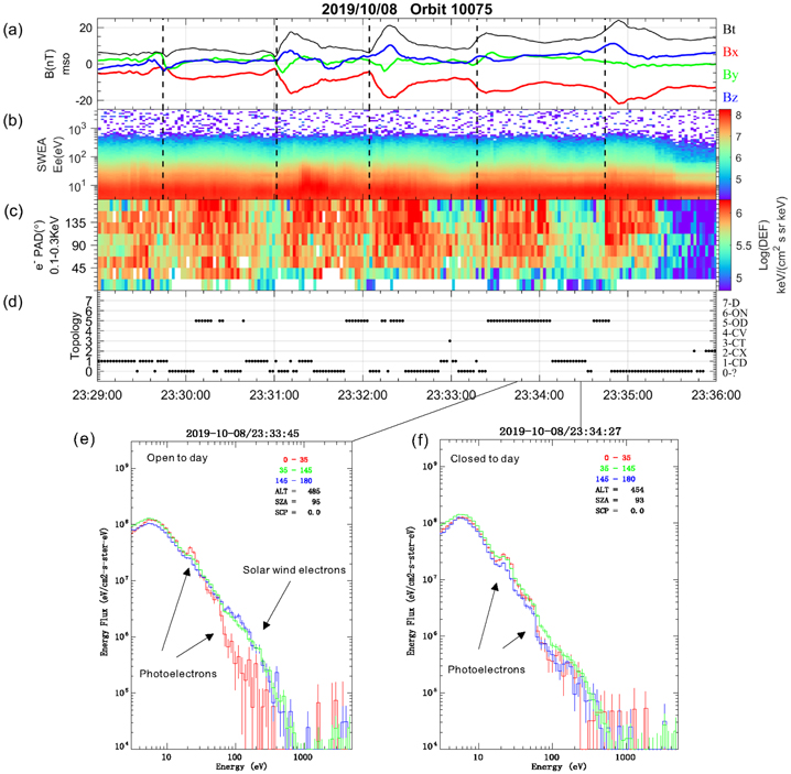
Figure 3. The electron distribution measured by SWEA. (a) The magnetic field. (b) The omnidirectional energy spectrum of electrons. (c) The electron pitch angle distribution within energy range 100–300 eV. (d) The topology index (0: unknown, 1: close-to-day (CD), 2: cross-terminator-closed (C-X), 3: closed-trapped (C-T), 4: closed-voids (C-V), 5: open-to-day (O-D), 6: open-to-night (O-N), 7: draped (DP)). (e) The typical electron distribution of open-to-day field lines. (f) The typical electron distribution of closed-to-day field lines.
Download figure:
Standard image High-resolution imageIt is clear from Figure 3(d), apart from the unknown types, the background magnetic field lines belong to the closed-to-day type. Open-to-day field lines appear when clouds are observed, suggesting that low-altitude clouds move tailward along open field lines, which is different from high-altitude clouds with draped field lines (Halekas et al. 2016). As mentioned, open-to-day field lines may also indicate the occurrence of magnetic reconnection between crustal field lines and the IMF. Therefore, characteristics of magnetic field topology variation in low-altitude clouds are hard to explain under the "snowplow" scenario of Halekas et al. (2016). Owing to open-to-day field lines in the clouds, the precipitation of solar wind electron flux—moving antiparallel to field lines—would generate an outward field-aligned current (Figure 3(e)), which may account for twisted field lines inside the clouds. Further, similar to the outflow at Earth's cusp, precipitation of solar wind plasma may transfer energy to the upper atmosphere, causing heating, dissociation, and ionization, and enhance ion supply (e.g., Xu et al. 2014) and ion outflow (Nilsson et al. 1994).
3. Discussion and Conclusion
In this study, we studied an event of periodic plasma clouds (period is about 70 s) at low altitude that was based on MAVEN observations of Mars. Using the "1/v" method, we found that the source of these low-altitude clouds was located at a low-altitude region (altitude is ∼120 km) where crustal fields could be intense. In these clouds, the average tailward flux of O+ was ∼2 × 107 cm−2 s−1 and for  , 6 ×107 cm−2 s−1, which is approximately an order of magnitude higher than the average loss of the Martian magnetotail (Nilsson et al. 2011, 2021; Brain et al. 2015; Dubinin et al. 2021; Inui et al. 2019). Thus, the clouds could significantly enhance the efficiency of plasma transport, particularly for the sequence of periodic clouds we reported here. However, only a single qualifying event with simultaneous signatures of magnetic field amplification, energy-dispersed ions and the open-to-day field lines, has been found during ∼6 yr MAVEN observations. The role plasma cloud played in the total ion escape is unclear without statistical study. Future statistical study is necessary to address the occurrence rate and spatial extent of the clouds to reveal their contribution to ion escape.
In comparison to the high-altitude clouds investigated by Halekas et al. (2016), we found that low-altitude clouds have many different characteristics: (1) enhancement of magnetic field in low-altitude clouds could be caused by compressional structures, while in high-altitude clouds it was induced by the shielding current in the boundary of clouds; (2) twisted magnetic field lines in our case could be driven by the field-aligned current, while it might be caused by boundary shear instabilities for Halekas et al. (2016). In our case, we also noticed (3) there is a mixture between solar wind ions and ionospheric ions inside clouds; (4) ionospheric ions with a different mass have the same velocity rather than the same energy; and (5) the magnetic field topology is of the open-to-day type. These last three characteristics are absent in the case of Halekas et al. (2016). Thus, Halekas et al.'s scenario for the high-altitude cloud formation (2016) is not applicable to the low-altitude clouds we survey here. There are two possible reasons for this difference. One is that low-altitude clouds may have the same source as high-altitude clouds but develop at an earlier stage. Low-altitude clouds could evolve into high-altitude ones. The second reason might be that they were generated by a different mechanism because they each have a different magnetic field topology. This issue could be clarified by multipoint spacecraft observations.
Energy-dispersed O+ and  (E > 30 eV) in clouds (Figures 1(g) and (h)) could be explained by two possible reasons. First, the group of ions could be initially in a homogeneous state at the source region. Due to some processes, some ions in the source accelerate and arrive at spacecraft earlier while other ions, which also accelerate but at a lower speed, arrive later. Because both O+ and
  have the same velocity at an instantaneous time, and the mixture of solar wind/ionospheric ions with open field lines are observed in the cloud, the process to energize the ions at the source could be a magnetic reconnection between the IMF and crustal fields (e.g., Hara et al. 2017; Harada et al. 2018). Magnetic reconnection could accelerate ionospheric plasma mass-independently (Speiser 1965), resulting in the outflow of O+ and
  at the same speed. Since outflow speed is proportional to the reconnection rate (e.g., Yamada et al. 2010), the signature of energy-dispersed ions may suggest that the reconnection rate was variable. Our "1/V" method inferred that the sources could be located in the ionosphere with altitude ∼120 km. Although magnetic reconnection might occur in the ionosphere, magnetic reconnection would be strongly suppressed by a collision resulting from being in such a low altitude (Cravens et al. 2020). Second, because ions behave similarly to the outflow from Earth's cusp (e.g., Yau & André 1997; Nilsson et al. 2006), they might be heated and widely energy-distributed in the source, thus spreading out according to their different velocities and causing energy dispersion. Away from the source, ions gradually become colder and evolve to dispersed ion beams (see Figure 7 of Nilsson et al. 2012). In this case, ions (O+ and
  ) with the same velocity would move together as measured instantaneously by the spacecraft. Given that solar wind electrons move along open field lines in clouds, we may suggest a scenario that accounts for this heating mechanism. Due to the interaction of the IMF with the crustal field, magnetic reconnection that occurs somewhere above the source region would open these lines, which would guide solar wind electrons to move downward (outward field-aligned currents) to the low altitude of ∼120 km. The precipitation of solar wind electrons could heat the low-altitude ionospheric plasma through collisions or wave–particle interaction (e.g., Nilsson et al. 1994, 2006; Yau & André 1997). Previous studies have demonstrated that wave–particle interaction triggered by field-aligned currents plays a role in plasma heating and acceleration in the low-altitude ionosphere of Mars (Ergun et al. 2006; Lundin et al. 2011). Considering that magnetic reconnection is rare in such an ionosphere, we think the heating mechanism better accounts for these low-altitude clouds.
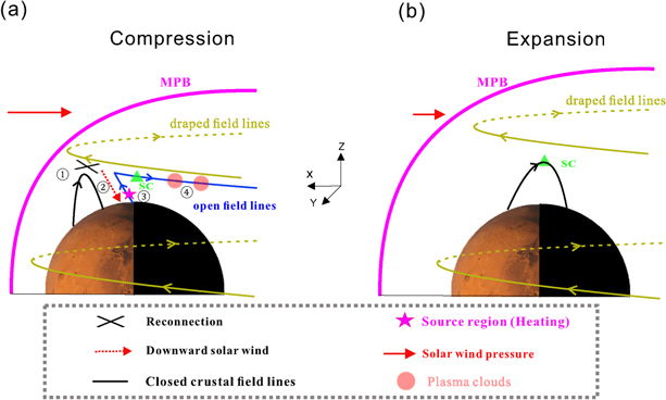
Additionally, from Figure 1, we notice that the appearance of energy-dispersed ions for each cloud was concurrent with the enhancement of magnetic field strength. Considering that magnetic reconnection between the IMF and the crustal field is required for the heating mechanism, this enhancement could be attributed to the compression of external solar wind, which triggers reconnection. Furthermore, although the spacecraft cannot measure the upstream IMF, the direction of draped field lines in the magnetosheath can be a proxy to the direction of upstream IMF (e.g., Fang et al. 2018; Ma et al. 2018). We find that the average magnetic field vectors (Bx, By, Bz) in the magnetosheath (during 2019-10-09 00:10-01:00) is (4.18, −12.47, −3.11) nT (not shown here), which indicates that the IMF is mainly oriented in the -Y direction, and these clouds located at the − E SW hemisphere ( E SW represents the solar wind electric field direction), impling a possibility that these clouds may be directed to return to the planet and may not be lost ultimately (Fang et al. 2010). In this case, we sketched a diagram to illustrate the full scenario for the observed sequence of periodical clouds (Figure 4); here the dynamic pressure of upstream solar wind assumes periodic variation. As shown in Figure 4(a), the Martian induced magnetosphere was compressed when the solar wind dynamic pressure was higher. In this case, the draped magnetic field and the density of background low-energy ionospheric ions would be enhanced due to compression (see Figures 1(d) and (i)). Compression thins the current sheet separating the IMF and the crustal field in the dayside ionosphere and triggers magnetic reconnection (Hara et al. 2017; Harada et al. 2018). This magnetic reconnection generates open field lines (Figure 3(d)) and facilitates the downward flow of solar wind electrons along them (Figure 3(e)), which results in the heating of plasma in the low-altitude source and leads to tailward moving plasma clouds. In contrast, the Martian magnetosphere would expand when solar wind dynamic pressure decreases (Figure 4(b)). That expansion would result in a decrease in magnetic field strength and in the density of background ionospheric plasma, as well as closed crustal field lines (see Figure 3(d)). Moreover, magnetic reconnection would cease due to thickening of the current sheet. Therefore, periodically varied dynamic pressure would lead to periodic magnetic reconnection, causing periodic heating and plasma clouds.
Figure 4. Diagrams to illustrate the generation of plasma clouds. Due to the compression of enhanced solar wind dynamic pressure (a), the magnetic reconnection between the draped lines and crustal field lines was triggered (①), which opens field lines facilitating the solar wind precipitation to low-altitude ionosphere (②) and causes plasma heating (③), finally generating plasma clouds moving tailward along open field lines (④). Due to the expansion of magnetosphere during the period of decreasing dynamic pressure (b), activities that trigger clouds cease.
Download figure:
Standard image High-resolution image
Future multipoint observations combining China's TIANWEN-1 (Wan et al. 2020), MAVEN, and Mars Express (Barabash et al. 2006) would provide a better opportunity to address the origin and evolution of plasma clouds, and its role in the ion escape.
All MAVEN data used in this paper are available from NASA's Planetary Data System (https://pds-ppi.igpp.ucla.edu/mission/MAVEN/MAVEN/). We would like to thank the entire MAVEN team for providing data access and support. Special thanks to Jasper Halekas, James P. McFadden, David Mitchell, and John E. P. Connerney for their contributions in making available data from SWIA, STATIC, SWEA, and MAG, respectively. This work is supported by the National Natural Science Foundation of China (grants 41922031, 41774188), the Strategic Priority Research Program of Chinese Academy of Sciences (grant No. XDA17010201), and the Key Research Program of the Institute of Geology & Geophysics, CAS, grant No. IGGCAS- 201904, IGGCAS- 202102. C.Z. is supported by a scholarship from China Scholarship Council (Student Number. 202104910297). K.L. is supported by a pre-research project on Civil Aerospace Technologies (No. D020104), which is funded by China's National Space Administration. We also thank Jasper Halekas, James P. McFadden, Lihui Chai, Xiaodong Wang, Stats Barabash, and Fang Qian for helpful discussion and encouragement.