


Abstract
Despite numerous observational and theoretical attempts, the heating problem of the solar chromosphere still remains unsolved. We develop a novel 3D two-fluid model that accounts for dynamics of charged species and neutrals, and use it to perform the numerical simulations of granulation driven jets and associated waves in a quiet region of the solar chromosphere. The energy carried by the waves is dissipated through ion–neutral collisions, which are sufficient to balance radiative energy losses and to sustain the quasi-stationary atmosphere whose ion and neutral number densities, ionization fraction, and temperature profiles are relatively close to the observationally based semi-empirical model. Additional verification of our results is provided by a good fit of the numerically predicted waveperiod variations with height to the recent observational data. These observational validations of the numerical results demonstrate that the wave heating problem of a quiet region of the chromosphere may be solved.
Export citation and abstract BibTeX RIS
1. Introduction
One of the central and long-standing problems of heliophysics concerns the source of thermal energy required to heat different layers of the solar atmosphere. It is observationally well established that the temperature raises with height in this atmosphere, which effectively radiates its energy away and therefore it must be heated by physical processes that still remain to be determined. Since the first atmospheric layer that is heated is the solar chromosphere, significant attention was given in the past to the heating processes in this layer (e.g., Ulmschneider et al. 1978; Carlsson & Stein 2002; Fawzy et al. 2002; Stein et al. 2009). The main result of these studies is that various waves produced in the solar convection zone propagate through the photosphere and chromosphere, and heat the latter by forming strong shocks that effectively dissipate their energy in the local medium. Observations of waves in the solar atmosphere clearly show that only waves of certain frequencies may reach the chromosphere because of cutoff frequencies (Wiśniewska et al. 2016; Kayshap et al. 2018). A theoretical prediction of the existence of cutoff for acoustic waves in the solar atmosphere was first made by Lamb (1911) and then extended to different waves by Edwin & Roberts (1982), Musielak et al. (1989), and many others.
More recently, Wójcik et al. (2018, 2019b) studied wave cutoffs in a more realistic solar chromosphere that accounts for partially ionized gases and interactions between ions (combined with electrons) and neutrals, which play a central role in dissipation of the energy carried by the waves and was predicted and estimated analytically by Vranjes & Poedts (2010). Additionally, Khomenko et al. (2018) and Martínez-Sykora et al. (2020) included ions and neutrals into their 2D and 3D numerical models of self-generated solar granulation. The contribution of neutrals was mimicked by amending extra terms in the induction equation. A 1D two-fluid model in which neutrals directly participate in dynamics of the atmosphere was developed by Kuźma et al. (2019), who used numerical simulations to demonstrate that wave damping is strong enough to heat the chromosphere by monochromatic acoustic waves with their waveperiods within the range of 30–200 s. In addition, Kuźma et al. (2017) explored the generation of two-fluid spicules, and Srivastava et al. (2018) proposed that two-fluid penumbral jets possess a sufficient energy to heat the 2D solar atmosphere. Also, Maneva et al. (2017) showed that two-fluid ion magnetoacoustic-gravity waves lead to local heating of a magnetic flux-tube. Popescu Braileanu et al. (2019) reported the two-fluid code for a partially ionized solar plasma, and Singh et al. (2019) developed a 2D model of reconnection in a solar magnetic current-sheet, taking into account the two-fluid effects of ionization and recombination. Moreover, Wójcik et al. (2020) performed 2D radiative numerical simulations of two-fluid waves that were generated by spontaneously evolving and self-organizing convection with granulation at their tops. It was found that a part of the energy carried by these waves is dissipated in ion–neutral collisions, which effectively heat the atmosphere.
Despite the recent studies mentioned above, the treatment of energy flow from deeper and cooler solar layers and the heating of the outer and hotter regions remains the main unsolved heating problem of quiet chromospheric regions. In this Letter, we develop a novel theory with the aim to explain the role of ion–neutral collisions in the process of the chromospheric heating, and propose to solve the problem. To achieve this goal, we perform for the first time 3D comprehensive numerical simulations of two-fluid jets and waves generated by granulation, and conversion of their energy into heat in a quiet region of the chromosphere. We present the numerical model in Section 2 and devote Section 3 to show and discuss the results of our numerical simulations. Finally, we conclude this Letter in Section 4.
2. Numerical Model
We consider a gravitationally stratified and partially ionized solar atmosphere, whose evolution is described by this set of radiative two-fluid equations (Leake et al. 2014; Maneva et al. 2017; Popescu Braileanu et al. 2019):


with the momentum collisional, Sm, and energy, Qi,n, source terms defined as

Here subscripts i, n, and e correspond respectively to ions, neutrals, and electrons;  denotes mass densities,
  number densities, μi = 0.58 and μn = 1.21 are the mean masses, which are taken from the OPAL solar abundance model (e.g., Vögler 2004), and mH is the hydrogen mass. The symbols
  are ion and neutral velocities,
  ion+electron and neutral gas pressures, B is the divergence-free (∇ · B = 0) magnetic field, which is controlled by the hyperbolic divergence-cleaning technique of Dedner et al. (2002), and
  are temperatures specified by ideal gas laws
Ion–neutral collision frequency is given as (Ballester et al. 2018)

with the collisional cross-section, σin, for which we choose its quantum value of 1.4 × 10⁻¹⁹ m2 (Vranjes & Krstic 2013). We set up a gravitational acceleration vector as g = [0, −g, 0] with its magnitude g = 274.78 m s−2. The symbol Lr denotes radiative loss term, which is implemented in the low atmospheric regions in the framework of Abbett & Fisher (2012) and as thin radiation in the top atmospheric layers (Moore & Fung 1972), γ = 1.4 is the specific heat ratio, kB is the Boltzmann constant, I is a unity matrix, and μ is magnetic permeability of the medium. The other symbols have their standard meaning.
3. Numerical Results
We perform both 3D and 2D numerical simulations with the JOANNA code (Wójcik et al. 2018, 2019a, 2019b, 2020), which features shock-capturing schemes based on Riemann solvers, such as HLLD (Miyoshi & Kusano 2005), for nonuniform rectangular grids. As we ran the 2D model for comparison purposes with the 3D case, we set exactly the same parameters in both the 3D and 2D systems.
Note that we validated the JOANNA code by performing a number of HD, MHD, and two-fluid tests. The results obtained so far with the use of this code (for two-fluid solar spicules and associated plasma outflows, Kuźma et al. 2017; for penumbral jets, Srivastava et al. 2018; for chromospheric heating by monochromatic acoustic waves, Kuźma et al. 2019; for convection and associated plasma blobs, Navarro et al. 2019; for atmospheric heating by granulation-excited magnetic-gravity waves and associated origin of the fast solar wind, Wójcik et al. 2020, 2019a) show that the code perfectly fits our requirements in solving the formidable task of numerical modeling (including 3D numerical simulations) of different two-fluid waves in a highly stratified and magnetically structured solar atmosphere.
We set the CFL number equal to 0.3, choose a second-order accuracy in space with linear reconstruction and in time with the Runge–Kutta method, and specify the 3D simulation box along horizontal (x), vertical (y), and transversal (z) directions as (−2.56 ≤ x ≤ 2.56) Mm × (−2.56 ≤ y ≤ 60) Mm × (−2.56 ≤ z ≤ 2.56) Mm. For the 2D simulations, we use the same settings along the x- and y-directions, and assume that the system is invariant along the z-direction. This box allows us to simulate the convectively unstable region below the photosphere that occupies the layer 0 < y < 0.5 Mm. Below the height y = 2.56 Mm, we set a uniform grid with cell size 20 km in each direction, while higher up we stretch the grid along the y−direction dividing it into 256 cells whose size steadily grows with height. At the bottom and top boundaries we fix all plasma quantities to their hydrostatic values, and allow ions and neutrals to enter the simulation box with their vertical velocities equal to 0.15 km s−1. The latter is estimated by requiring that outflowing mass flux is balanced by the inflowing mass flux that is set at the bottom boundary. We set all four side boundaries as periodic.
We start the numerical simulations at t = 0 s by setting hydrostatic ion and neutral number densities (Figure 1, the top and middle rows, dotted lines) and gas pressures (not shown) profiles, which are specified by the semi-empirical temperature model of Avrett & Loeser (2008). In this model we take equal ion and neutral temperatures, Ti(y) = Tn(y) (Figure 2, dotted lines); for details, see Wójcik et al. (2020). This initial state is identical to that used by Wójcik et al. (2020) in their 2D simulations with the only exception that here the atmosphere is initially (at t = 0 s) permeated by a vertical magnetic field of 5 G. Note that the initial profiles of ion number density, ni(y) (Figure 1, top), and neutral number density, nn(y) (Figure 1, middle), show similar height variations as those of Figure 8 of Avrett & Loeser (2008). However, the ion profile does not exhibit the local minimum at y ≈ 0.9 Mm, which is present in the data of Avrett & Loeser (2008); to obtain such a minimum  must be taken into account (Kuźma et al. 2017).

Figure 1. Range of temporal changes (between minima and maxima at a given height y) of horizontally averaged <ni> (top), <nn> (middle), and <nn/ni> (bottom) with their averaged values (light-blue lines) for 3D (left) and 2D (right) cases. The initial (at t = 0 s) plasma quantities resulting from the temperature model of Avrett & Loeser (2008) are displayed by white dashed lines.
Download figure:
Standard image High-resolution image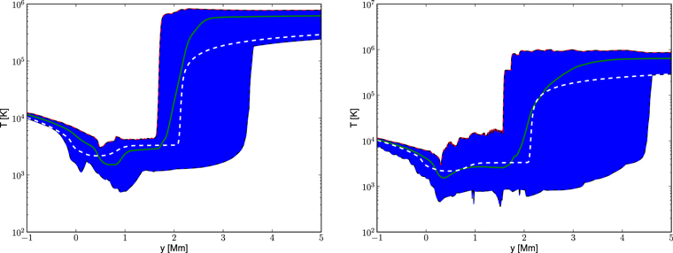
Figure 2. Range of temporal changes of horizontally averaged <Ti> for 3D (left) and 2D (right) cases. The initial ion and neutral temperatures of Avrett & Loeser (2008) are taken to be equal, Ti(y) = Tn(y), and they are illustrated on both panels by white dashed lines. Solid lines correspond to averaged values of <Ti> .
Download figure:
Standard image High-resolution imageAs the plots of Figure 1 demonstrate, there is also some discrepancy between the numerical results and those given by the semi-empirical model for y larger than 2 Mm, and this discrepancy is more prominent for our 2D models than for the 3D models. One main reason could be the assumed equality of Ti(y) and Tn(y), which alters the numerical results higher in the solar atmosphere, and another reason is the fact that the processes of ionization and recombination are not accounted for in our current models (e.g., Martínez-Sykora et al. 2020). To justify our assumption Ti(y) = Tn(y), we point out that the equal temperatures are often adopted in the literature (e.g., Zaqarashvili et al. 2011; Oliver et al. 2016; Ballester et al. 2018) and that a choice of the initial state does not play any major role in development of the system, but it results in its faster convergence (through a transient phase) to a quasi-equilibrium at which the plasma quantities are usually altered in comparison to their initial values (M. Schüssler 2015, private communication); for this reason, we consider Ti(y) = Tn(y) in the results presented in this Letter.
In order to seed convective instabilities, we launch at t = 0 s from the bottom of the photosphere a small (102 m s−1) random signal in vertical components of ion, Viy, and neutral, Vny, velocities. Then, we let the system self-evolve in time without action of any external source. As the system is convectively unstable for y < 0, the instabilities generate the solar granulation with its typical characteristics such as downdrafts, updrafts, and granules (Wójcik et al. 2020, Figures 4 and 5). This granulation reshuffles magnetic field lines in the photosphere and excites two-fluid jets and associated waves (Kuźma et al. 2017), which are well seen in profiles averaged over the whole horizontal direction vertical component of ion speed, <Viy> (Figure 3, top). Note that the code was run until t = tmax = 5 · 103 s. The system evolved through its transient phase (not shown), and well below tmax it reached its quasi-stationary state with the ion temperature minimum located in 3D at y ≈ 0.8 Mm and in 2D at y ≈ 0.5 Mm (Figure 2). Vertical ion flow and transition region oscillations are seen smaller in 3D (left panels) than in 2D (right panels).
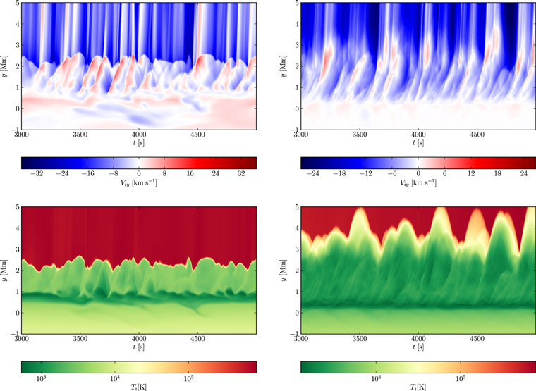
Figure 3. Time–distance plots of horizontally averaged vertical component of ion velocity (top) and ion temperature (bottom) for 3D (left) and 2D (right) cases.
Download figure:
Standard image High-resolution imageFigure 4 illustrates waveperiods (contour plots) obtained from the Fourier power spectrum of <Viy> . The Fourier transform is made of time signatures of the vertical component of horizontally averaged ion velocity, displayed in Figure 3 (top), and collected for each height y. These waveperiods are compared to the observational data of Wiśniewska et al. (2016) and Kayshap et al. (2018). It is seen that the comparison presented in Figure 4, which displays the wave power at different periods and atmospheric heights, approximately corresponds to the location of the observationally established wave power. This agreement confirms that ion–neutral collisions are efficient energy release processes, resulting in the kinetic energy dissipation and its convertion into heat.

Figure 4. Waveperiods, P, evaluated from Fourier power spectrum for ion vertical velocity, <Viy> , displayed in the top panels of Figure 3 (contour plots). The diamonds and dots show the observational data obtained by Wiśniewska et al. (2016) and Kayshap et al. (2018) for 3D (left) and 2D (right) cases, respectively.
Download figure:
Standard image High-resolution image
Indeed, Figure 3 (bottom) shows that these collisions lead to the atmosphere with the transition region located around y = 2.1 Mm in the 3D case (left) and y = 2.5 Mm in the 2D case (right). This serves as more evidence that the atmosphere reached its quasi-equilibrium at which collisional heating balances the radiative cooling. As a result, the numerically obtained and averaged over the horizontal direction vertical profiles of ion, <ni> (Figure 1, top), and neutral, <nn> (Figure 1, middle), number densities, ionization factor, <nn/ni> (Figure 1, bottom), and ion temperature, <Ti> (Figure 2), closely resemble the initially imposed, semi-empirical model of Avrett & Loeser (2008).
4. Conclusions
We performed numerical simulations excited by the granulation two-fluid jets and waves in a partially ionized solar atmosphere taking into account ion–neutral collisions. The considered neutral acoustic-gravity and ion magneto-gravity waves were generated by naturally evolving convection. We found that the waveperiod variation with height is relatively close to the observational data of Wiśniewska et al. (2016) and Kayshap et al. (2018). A part of energy carried by these waves is dissipated by ion–neutral collisions in the chromosphere. This dissipation results in thermal energy release and it leads to the solar atmosphere with its ion and neutral number densities, ionization, and temperature vertical distributions essentially fitting the semi-empirical model of Avrett & Loeser (2008).
Since this is the first time when the agreement with the observationally based model data was obtained, we conclude that our 3D results may unravel the main mechanisms of the wave heating of the quiet regions of the chromosphere, which are collisions between neutrals and ions. Such a process was also studied within the 2D two-fluid framework, neglecting the dependence on the transversal coordinate. In comparison to the 2D findings the 3D effects lead to the atmosphere with a vertical temperature profile, which better fits the semi-empirical data of Avrett & Loeser (2008), and the vertical variations of waveperiods of the excited two-fluid waves are closer to the observational data of Wiśniewska et al. (2016) and Kayshap et al. (2018). Some discrepancies between the numerical predictions and that of the empirical data are likely caused by the lack of ionization/recombination (e.g., Martínez-Sykora et al. 2020) in the model considered in this Letter.
The 3D JOANNA code was developed by Darek Wójcik. This work was done within the framework of the project from the Polish Science Center (NCN) grant Nos. 2017/25/B/ST9/00506 and 2017/27/N/ST9/01798.