Magnetospheric Multiscale Observations of Electron Vortex Magnetic Hole in the Turbulent Magnetosheath Plasma

Turbulence is a ubiquitous feature of various space and astrophysical plasmas that include the solar wind, the planetary magnetospheres (including magnetotail and magnetosheath), the interstellar medium, and accretion flows (e.g., Tu & Marsch 1995; Bruno & Carbone 2005; Sahraoui et al. 2006, 2009, 2010, 2013; Schekochihin et al. 2009; Huang et al. 2012, 2014a, 2017; Hadid et al. 2015; Breuillard et al. 2016). A nonlinear energy cascade in magnetized turbulent plasmas leads to the formation of different coherent structures such as mirror modes (Sahraoui et al. 2004, 2006), magnetic islands/flux ropes (e.g., Daughton et al. 2011; Fu et al. 2013; Markidis et al. 2013; Karimabadi et al. 2014; Huang et al. 2014b, 2014c, 2015, 2016a, 2016b), current sheets, and other discontinuities (e.g., Retinò et al. 2007; Osman et al. 2012; Wang et al. 2013; Chasapis et al. 2015; Yang et al. 2015). These coherent structures are thought to play an important role in dissipating energy and transporting particles in turbulent plasmas (e.g., Drake et al. 2006; Sundkvist et al. 2007; Servidio et al. 2014; Zhang et al. 2015; Fu et al. 2017).

Recent two-dimensional and three-dimensional particle in-cell (PIC) simulations by Haynes et al. (2015) and Roytershteyn et al. (2015) have revealed the existence of a new type of nonlinear coherent structure in turbulent magnetized plasmas, which is referred to as an electron vortex magnetic hole. Those simulations include the following basic properties of the electron vortex magnetic hole: size of the order of the electron-scale, quasi-circular cross-section, a trapping of electrons to form the electron vortex, and an electron perpendicular temperature larger than the parallel one.

Magnetic holes with significant magnetic field depression (or reduction) have been reported in the solar wind (e.g., Turner et al. 1977; Zhang et al. 2008), in the magnetosheath (e.g., Tsurutani et al. 2011; Yao et al. 2017), and in the magnetotail plasma sheet (e.g., Ge et al. 2011). Recently, sub-proton-scale magnetic holes were detected in the magnetotail using the data of THEMIS, Cluster, and Magnetospheric Multiscale (MMS) missions (e.g., Sun et al. 2012; Sundberg et al. 2015; Gershman et al. 2016; Goodrich et al. 2016a, 2016b). However, before the launch of MMS the low time resolution of particle data limited the characterization of magnetic holes and did not allow us to accurately identify electron vortex magnetic holes. In this Letter, we provide for the first time a new and direct evidence of the existence of an electron vortex magnetic hole in the turbulent magnetosheath plasma thanks to the unprecedented high time resolution data of the MMS mission (Burch et al. 2016).

The MMS spacecraft, launched in 2015 March, consists of four identical spacecraft that provide unprecedented high time resolution of the plasma data. We use the magnetic field data from the Fluxgate Magnetometer sampled at 8 Hz (survey mode) or 128 Hz (burst mode; Torbert et al. 2014), and the 3D particle velocity distribution functions and the plasma moments from the Fast Plasma Instrument sampled at 30 ms (resp. 4.5 s) for electrons and 150 ms (resp. 4.5 s) for ions in burst mode (resp. fast mode; Pollock et al. 2016).

Figure 1 exhibits an overview of MMS multiple crossings of the magnetosheath and the bow shock on 2015 October 25. Since the separation between the four MMS spacecraft (∼15 km) is much shorter than the characteristic scales of the magnetosheath and bow shock, the MMS spacecraft see nearly the same large-scale features of magnetosheath and bow shock structures. For this reason we show only data from MMS1 in Figure 1. Figures 1(a)–(f) show that the magnetosheath is highly variable with large magnetic field fluctuations, slow ion velocity, and higher ion density as compared with the solar wind, and with typical magnetosheath ion energies between ∼100 eV and several keV and electron energies between tens of eV and hundreds of eV. During the period from 08:40 UT to 09:40 UT, MMS crossed the bow shock four times (marked by blue dashed lines) and stayed in the magnetosheath in the time periods marked by red bars on the top of Figure 1 (the solar wind or foreshock periods are marked by black bars on the same figure). Figures 1(g)–(i) provide a short period (35 s) of observations in the magnetosheath. They show the presence of a magnetic hole with a magnetic depression marked by two black dashed lines.

Zoom In Zoom Out Reset image size

Magnetic power spectral density (PSD) calculated in an interval of time of ∼100 s that included the observed magnetic hole was examined (see Figure 5 in the Appendix). It is found to be broadband and characterized by two ranges having a power-law separated by a spectral break near the local ion scale ∼1 Hz. This spectrum is similar to the previous observations of the turbulence in magnetosheath and in the solar wind (e.g., Leamon et al. 1999; Sahraoui et al. 2006, 2010, 2013; Alexandrova et al. 2008; Huang et al. 2017). Power-law fits yielded slopes close to −1.64 in f < 0.8 Hz and −2.97 for 1 Hz < f < 10 Hz. Furthermore, the development of intermittency characterized by the heavy tails in the probability distribution functions (PDFs) of the magnetic field increments at small scales (see Figure 5 in the Appendix), which is evidence of the existence of a fully developed turbulence that leads to the generation of intermittent structures at small scales. These observations indicate that the magnetic hole was embedded in a background of turbulent fluctuations that cover a broad range of scales, similarly to the numerical simulations of decaying turbulence of Haynes et al. (2015) and Roytershteyn et al. (2015).

Figure 2 gives detailed observations of the magnetic hole from 08:48:46 UT to 08:48:48 UT. All the data are presented in the LMN coordinates, which were determined by minimum variance analysis of the magnetic field from MMS1 (08:48:46.986–08:48:47.144 UT) (Sonnerup & Scheible 1998, pp. 185–220). In this coordinate system, the maximum variation direction ${\boldsymbol{L}}$ = [−0.33, 0.75, 0.58] (GSE) that can be considered as the axis of the magnetic hole, the intermediate variation direction ${\boldsymbol{M}}$ = [0.81, −0.09, 0.58] (GSE), and the minimum variation direction ${\boldsymbol{N}}$ = [−0.48, −0.66, 0.58] (GSE). MMS3, MMS1, and MMS2 successively detected a reduction in the magnetic field strength (Figure 2(a)) that is essentially due to the field-aligned component (Figure 2(b)) around 08:48:47 UT. The magnetic depletion is up to 77% on MMS1, which we refer to as a magnetic hole. Figures 2(e)–(l) display the electron observations from the four spacecraft. The electron density (Figure 2(e)) and electron temperature increase (Figure 2(f)) inside the magnetic hole. However, the electron parallel temperature (with respect to the ambient magnetic field) decreases (Figure 2(g)), while the electron perpendicular temperature increases (Figure 2(h)). MMS1 observed the strongest reduction in magnetic field along with the strongest decrease of the electron parallel temperature and the strongest increase of the electron perpendicular temperature. During the crossing of the magnetic hole, the electron velocities in V_em component (Figure 2(k)) exhibited a bipolar variation, namely, V_em changes from reverse to along ${\boldsymbol{M}}$-direction, implying the possible existence of an electron vortex structure in the M–N plane inside the magnetic hole. By combining the different variations of the V_en component (Figure 2(l)) on the different spacecraft (e.g., the increase of ∣V_en∣ seen by MMS1, and the decrease of ∣V_en∣ seen on MMS2 and MMS3) and the large ambient electron flow V_en, the magnetic hole can be interpreted as an electron vortex imbedded in the ambient plasma flow. In this scenario, one may infer that MMS1 was crossing one-half of the electron vortex with negative V_en in the frame of the moving hole, while MMS2 and MM3 were crossing the other half with positive V_en in this moving frame. We will return to this point at the end of this Letter.

Zoom In Zoom Out Reset image size

Figure 3 shows the currents and electron pitch angle distributions associated with the magnetic hole from MMS1 and MMS3. The pitch angle distribution from 2 to 30 keV is not presented because the fluxes at these high energies are too low. The current is estimated at each spacecraft using the plasma measurements (i.e., ${\boldsymbol{J}}={ne}({{\boldsymbol{V}}}_{{\rm{i}}}-{{\boldsymbol{V}}}_{{\rm{e}}})$, where n is the plasma density, e is the electric charge, ${{\boldsymbol{V}}}_{{\rm{i}}}$ is the ion flow, and ${{\boldsymbol{V}}}_{{\rm{e}}}$ is the electron flow). All current components in Figures 3(b) and (f) are intense in the magnetic hole. In addition, we also estimated the current using the Curlometer method (Dunlop et al. 2002) and the electron current ${{\boldsymbol{J}}}_{{\rm{e}}}=-{ne}{{\boldsymbol{V}}}_{{\rm{e}}}$ (not shown here). We found one bipolar signature in the J_m component from both the Curlometer method and from the plasma measurements (Figures 3(b) and (f)), which is similar but with an opposite sign than the electron velocity component V_em in Figure 2(k). We deduce that electrons carry most of the electric current inside the magnetic hole. MMS1 observed a dip in the total current in the middle and a peak in the outer region of the magnetic hole (Figure 3(b)), while MMS3 detected only one peak of the current (Figure 3(f)). Recent 2D and 3D PIC simulations showed that there is one dip in the core region and peaks at the edge of magnetic hole (Figure 3 in Haynes et al. 2015 and Figure 8 in Roytershteyn et al. 2015). Thus, the observed features of the current by MMS1 and MMS3 in our event may be explained their different trajectories when they crossed the magnetic hole. In other words, MMS1 may have crossed the core region of the magnetic hole while MMS3 may have encountered the edge the observed magnetic hole.

Zoom In Zoom Out Reset image size

The electron spectrogram does not show clear flux enhancement at high energies (>600 eV) in the magnetic hole. Electrons behave differently inside and outside the magnetic hole. Bidirectional electrons are observed in the energy range 0–0.2 keV (Figures 3(e) and (i)), while anti-parallel electron flows are seen in the energy range 0.2–2 keV outside the magnetic hole (Figures 3(d) and (h)). The electrons have a similar behavior inside the magnetic hole, except for the very clear enhancement in fluxes at ∼90° pitch angle in the energy range 0–2 keV. We deduce that these 90° pitch angle electrons are trapped and form an electron vortex within the magnetic hole. Note that very slight depressions in the magnetic field strength are detected before the magnetic hole (i.e., around 08:48:46.7 UT). These are also accompanied with flux enhancement around 90° pitch angles, suggesting that MMS observed a similar vortex structure at that time.

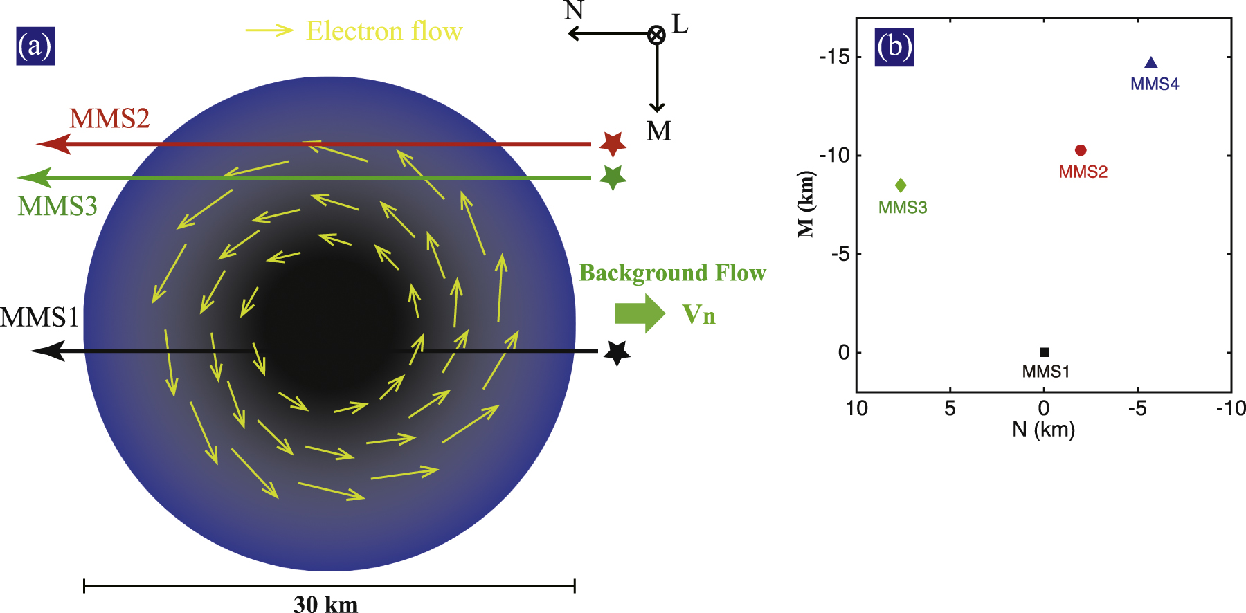
Figure 4 provides a schematic of the observed magnetic hole by MMS. Figure 4(a) draws the nearly circular cross-section geometry of the magnetic hole, while Figure 4(b) presents the positions of the four spacecraft in the M–N plane (perpendicular to the axis of the magnetic hole). Given the average background velocities in Figures 2(k) and (l), V_en ∼ −150 km s⁻¹ and V_em ∼ 0 km s⁻¹, the magnetic hole was moving opposite to the ${\boldsymbol{N}}$-direction. MMS3 was located in to the most left in the ${\boldsymbol{N}}$direction, and MMS1 was in between MMS3 and MMS2 in the ${\boldsymbol{N}}$direction, ensuring the successive encounters of MMS3, MMS1, and MMS2 with the magnetic hole (their trajectories are marked by three horizontal colored arrows in Figure 4(a)). Moreover, the magnetic hole is expected to be in the form of a counterclockwise vortex formed by the electron flow, leading to variations of V_emon MMS3, MMS1, and MMS2 from negative to positive direction, as well as a decrease in ∣V_en∣ for MMS3 and MMS2 and an increase in ∣V_en∣ for MMS1 (Figures 2(k)–(l)).

Zoom In Zoom Out Reset image size

In order to estimate the scale of the magnetic hole in the M–N plane, we assume that the magnetic hole moves with the ambient plasma flow (Sun et al. 2012). One can see that the electron velocity outside the magnetic hole is rather steady (Figures 2(i)–(l)). Therefore, the width of the magnetic hole in the ${\boldsymbol{N}}$ direction D_N is about 30 km using the equation D_N = ∣V_en∣ × dt, where dt ≈ 0.2 s is the duration of the crossing of the magnetic hole for MMS1. The estimated size D_N is about 0.23 ρ_i (∼30 ρ_e), where ρ_i and ρ_e are the proton and electron gyroradius (ρ_i ∼ 127 km and ρ_e ∼ 1 km based on ∣B∣ ∼ 20 nT, n ∼ 53 cm⁻³, T_i ∼ 310 eV, and T_e ∼ 33 eV). The width in the ${\boldsymbol{M}}$ direction can be estimated using the separation between the MMS spacecraft as shown in Figure 4(b). Considering the dip in the total current and the strong J_n component when J_m = 0, we can deduce that MMS1 crossed the core region when the current has dip, but did not cross the center point of the magnetic hole. MMS4 is located outside of the edge of the magnetic hole since it observed a slight decrease in B_t, yielding a maximum possible width of ∼30 km in the M direction. This suggests that the electron-scale electron vortex magnetic hole has a quasi-circular cross-section in the M–N plane.

Since there is a large V_el velocity of the background magnetosheath, the satellites moved some distance along the L-axis as well. Thus, we should note that we presented the electron vortex in the cross-section plane in Figure 4(a) based on the assumption of homogenous dimensions along the L-axis. Noting a strong J_l component of the current at J_m = 0, the electron vortex may be helical. Due to limitations in the observations (i.e., only two spacecraft observed very clear magnetic depression of magnetic hole), we could not determine the full 3D structure of the magnetic hole.

Small-scale magnetic holes with scales comparable to the proton gyroradius have been only observed in the magnetospheric plasma sheet (e.g., Sun et al. 2012; Sundberg et al. 2015; Gershman et al. 2016; Goodrich et al. 2016a, 2016b). However, similar observations could not have been made in the solar wind and magnetosheath because of the limited time resolution of the particle instruments, especially the electron measurements (particle characteristic scales in the latter regions are about 10 times smaller). An electron anisotropy with an enhancement in the perpendicular energy fluxes at 90° pitch angles was observed in some magnetic holes (Sun et al. 2012; Sundberg et al. 2015; Gershman et al. 2016). In our work, using the high time resolution data from MMS, we also found an enhancement of energy flux at pitch angles 90° inside an electron-scale magnetic hole in the turbulent magnetosheath plasma. This implies that small-scale magnetic holes show similar electron behaviors in these different plasma environments. Goodrich et al. (2016a) have reported that the Hall electron currents are responsible for the depression of magnetic field in the magnetic holes. Goodrich et al. (2016b) mainly focused on the electric field of the magnetic holes, including the major magnetic hole and a secondary magnetic hole with slight depression of ∼20% and short duration of ∼0.5 s. Using the high time resolution particle data from MMS, Gershman et al. (2016) have found that the currents carried by the electrons can be sufficient to account for depression of magnetic field in the magnetic hole. However, they observed the magnetic holes under the condition of electron temperature isotropy (T_e⊥ ∼ T_e∣∣ ) inside of the magnetic hole, which contrasts with the present observations (i.e., T_e⊥/T_e∣∣ ∼ 1.2). As for the background plasma, the magnetic holes in the two studies were detected under similar electron plasma temperature conditions (T_e∣∣ > T_e⊥), which may imply that both of them are be formed by the same mechanism.

Our analysis indicates the existence of an electron vortex magnetic hole in a turbulent plasma where the ambient plasma has T_e∣∣ > T_e⊥. The observed features, including density, electric current, electron temperature, electron vortex structure, trapped 90° pitch angle electrons, and background turbulent plasma with T_e∣∣ > T_e⊥, are well consistent with the predictions given by the simulations (Haynes et al. 2015; Roytershteyn et al. 2015). Thus, the observed magnetic hole can be explained by the simulations of Haynes et al. (2015) and Roytershteyn et al. (2015).

Other generation mechanisms have been proposed for small-scale magnetic holes, including electron mirror mode or field-swelling instabilities (e.g., Gary & Karimabadi 2006; Pokhotelov et al. 2013), tearing modes (Balikhin et al. 2012), and solitary waves (e.g., Baumgärtel 1999; Stasiewicz et al. 2003; Li et al. 2016; Yao et al. 2016). However, there are inconsistencies between the basic assumptions of the aforementioned mechanisms and the present observations. For example, in our event we have T_i/T_e ∼ 9.4 ≫ 1 (T_i ∼ 310 eV and T_e ∼ 33 eV) and T_e⊥/T_e∣∣ ∼ 0.84 < 1 for the background plasma, which do not fulfill the theoretical threshold of the electron mirror instability (T_e⊥/T_e∣∣ > 1 + 1/β_e⊥) and field-swelling instabilities (T_e > T_i) (e.g., Gary & Karimabadi 2006; Pokhotelov et al. 2013). The tearing mode may occur in localized regions of the cross magnetotail current sheet and is thought to result in isotropic electrons in the magnetic hole (Balikhin et al. 2012), which is inconsistent with anisotropic electron distributions inside the observed magnetic hole in the present study. Finally, the solitary wave theory is mainly appropriate in the weak nonlinear regime (Li et al. 2016; Yao et al. 2016), but may not be suitable for the strong nonlinear state of the magnetic hole in the magnetosheath turbulent plasma where magnetic field and plasma flow have large amplitude fluctuations.

In summary, we presented the detailed analysis of an electron vortex magnetic hole with a scale smaller than the proton gyroradius in the magnetosheath turbulent plasma using the MMS data. The magnetic hole has an electron-scale quasi-circular cross-section with a radius of 0.23 ρ_i. It is characterized by electron density and temperature increases, with an electron parallel temperature decrease but a perpendicular temperature increase (T_e⊥ > T_e∣∣ ) inside the magnetic hole. The current density has a dip in the center of the magnetic hole and a peak at its outer edge. Electrons are trapped inside the magnetic hole, and form an electron vortex in the cross-section plane with an enhancement in the perpendicular electron flux at 90° pitch angles. All these observational features are well consistent with the reported features of electron vortex magnetic hole from the kinetic simulations of Haynes et al. (2015) and Roytershteyn et al. (2015). Our observations demonstrate that the coherent structures behaving as electron vortex magnetic holes can be generated in space plasma turbulence.

We thank the entire MMS team and instrument leads for data access and support. This work was supported by the National Natural Science Foundation of China (41374168, 41404132, 41574168, 41674161), Program for New Century Excellent Talents in University (NCET-13-0446), and China Postdoctoral Science Foundation Funded Project (2015T80830). S.Y.H. and F.S. acknowledge financial support from the project THESOW, grant ANR-11-JS56-0008, and from LABEX Plas@Par through a grant managed by the AgenceNationale de la Recherche (ANR), as part of the program "Investissementsd'Avenir" under the reference ANR-11-IDEX-0004-02. Data are publicly available from the MMS Science Data Center at http://lasp.colorado.edu/mms/sdc/. Work at IRAP was supported by CNES and CNRS.

The magnetosheath is known to be one of the most turbulent regions of space (it is even more turbulent than the solar wind). The origin of that turbulence is still debated, but there are at least two major sources that work together and generate turbulence: the dynamical pressure of the solar wind and its interaction with the bow shock (large-scale driving; Karimabadi et al. 2014) and plasma instabilities due to temperature anisotropy (small-scale driving; e.g., Sahraoui et al. 2006). Huang et al. (2017) have recently conducted a large survey of the Cluster data (3 years) that provided the first complete picture of magnetosheath turbulence at MHD and kinetic scales. In the Letter, we did not address the turbulence properties in that general sense, but we rather focus on the evidence of electron-scale magnetic holes. Here, we show that the identified magnetic hole is not an isolated structure but it is rather embedded in a background turbulence that covers a broad range of scales. This can be seen in the plot below showing the analyzed waveforms (Figure 5(a)) and the corresponding power spectrum density (PSD; Figure 5(b)). The PSD has the classical features of turbulence (Figure 5(b)): a power-law spectrum at MHD scales with a slope close to −5/3 as predicted by MHD turbulence theories, a break near the ion scale (∼1 Hz), followed by a steeper power-law spectrum at sub-ion scales with a slope close to −2.97. These features are very similar to those reported in turbulence studies in the magnetostheath (e.g., Sahraoui et al. 2006; Alexandrova et al. 2008; Huang et al. 2014a, 2017; Hadid et al. 2015; Breuillard et al. 2016) and in the solar wind (e.g., Leamon et al. 1998; Sahraoui et al. 2009, 2013). Furthermore, Figure 5(c) shows the development of intermittency characterized by the heavy tails in the PDFs of the magnetic field increments at small scales. This is evidence of the existence of a fully developed turbulence that leads to the generation of intermittent structures at small scales. Thus, there is no doubt that turbulence is present in our data similarly to the simulation of Haynes et al. (2015) and Roytershteyn et al. (2015). However, the question as to whether turbulence is decaying or is driven cannot be answered in spacecraft data. This question can be studied only in numerical simulations of turbulence through the change in the initial/boundary condition from driving to decaying, and examining whether the turbulence properties depend or not on the simulation set up.

Zoom In Zoom Out Reset image size