


Abstract
The discovery of Kepler 452b is a milestone in searching for habitable exoplanets. While it has been suggested that Kepler 452b is the first Earth-like exoplanet discovered in the habitable zone of a Sun-like star, its climate states and habitability require quantitative studies. Here, we first use a three-dimensional fully coupled atmosphere–ocean climate model to study the climate and habitability of an exoplanet around a Sun-like star. Our simulations show that Kepler 452b is habitable if CO2 concentrations in its atmosphere are comparable or lower than that in the present-day Earth atmosphere. However, our simulations also suggest that Kepler 452b can become too hot to be habitable if there is the lack of silicate weathering to limit CO2 concentrations in the atmosphere. We also address whether Kepler 452b could retain its water inventory after 6.0 billion years of lifetime. These results in the present Letter will provide insights about climate and habitability for other undiscovered exoplanets similar to Kepler 452b, which may be observable by future observational missions.
Export citation and abstract BibTeX RIS
1. Introduction
Kepler 452b is the first super-Earth exoplanet discovered in the habitable zone (HZ) around a Sun-like star (Jenkins et al. 2015). It has a radius about 1.6 times that of Earth, orbits its primary with a distance slightly greater than that between the Sun and Earth, and receives 10% more stellar radiation flux than the Earth does from the Sun. Kepler 452b's parent star (Kepler 452) is a G-type star, like the Sun. The star is about 1.5 billion years older and about 20% more massive than the Sun. Unlike previously discovered exoplanets in the HZ of M dwarfs, which are too close to their parent stars and thus likely lack water (Lissauer 2007; Luger & Barnes 2015; Tian & Ida 2015) or could suffer intense flares and extreme ultraviolet radiation from M dwarfs (Lammer et al. 2007; Scalo et al. 2007), Kepler 452b does not have to face such problems. All these make Kepler 452b the most Earth-like habitable exoplanet if it is a rocky planet.
Because the mass of Kepler 452b is not measured, it is unknown whether Kepler 452b is a rocky planet or not. According to the statistics of the mass–radius relationship derived from observational samples with a radius less than 4 Earth radii (Weiss & Marcy 2014; Rogers 2015), the posterior predictive probability that Kepler 452b is a rocky planet with a thin atmosphere is between 49% and 62% (Jenkins et al. 2015). Thus, it is also possible that Kepler 452b is a planet with a small rocky core and a thick gaseous envelope. Nevertheless, Kepler 452b deserves detailed study because it is the closest analog to Earth known so far, and its present-day climate environment may represent that which our own Earth will experience in the future as the Sun brightens. Even if Kepler 452b turns out to be mostly gaseous, studies of Kepler 452b shall provide insights about climate and habitability for other undiscovered rocky exoplanets that have similar planetary radii and atmospheres.
While simple estimates suggested that Kepler 452b lies in the HZ of a Sun-like star (Jenkins et al. 2015), whether its climate is able to support life requires quantitative studies with more sophisticated models. Specifically, planetary surface temperatures are determined not only by the distance between planets and their primaries but also by greenhouse gas (GHG) concentrations in their atmospheres. If GHG concentrations are too low, a planet in the HZ could experience runaway freezing through the positive ice-albedo feedback. An example is our own home planet that experienced global glaciations and became a snowball about 2.3 and 0.6–0.7 billion years ago due to large decreases of GHG concentrations (Kirschvink 1992; Hoffman et al. 1998; Liang et al. 2006; Kopp et al. 2005). On the other hand, if GHG concentrations are too high, the surface temperature of the planet could be too high and become uninhabitable.
For Earth, the carbon dioxide (CO2) concentration in the atmosphere is limited by the carbonate–silicate cycle, which acts as a negative feedback mechanism to stabilize Earth's climate (Walker et al. 1981). If super-Earth exoplanets, such as Kepler 452b, are partially ocean-covered planets like our own Earth, as suggested by Cowan & Abbot (2014), carbonate–silicate weathering reactions over continents are able to keep atmospheric CO2 not very high. However, it was also suggested that super-Earth exoplanets such as Kepler 452b are likely aquaplanets with extensive oceans (Lissauer 1999), and whether and how silicate weathering works on aquaplanets are unknown. On the one hand, it has been speculated that aquaplanet atmospheres could have high-level CO2 because silicate weathering occurs most efficiently on exposed landmasses, suggesting that aquaplanets where all continents are submerged may not be able to efficiently recycle CO2 (Selsis et al. 2007). On the other hand, it has also been conjectured that CO2 concentrations could be limited by sea-floor silicate weathering (Pierrehumbert et al. 2011). Thus, Kepler 452b might experience the snowball state if sea-floor silicate weathering is sufficiently efficient, and it might also be too hot to be uninhabitable in the absence of silicate weathering. One of the purposes of the present Letter is to study Kepler 452b's climate states and habitability for extreme low and high CO2 concentrations.
Because Kepler 452b is about 1.5 billion years older than Earth and it receives 10% more stellar radiation (Jenkins et al. 2015), an important question is whether Kepler 452b had lost all its water through escape processes during its lifetime, especially if it has a much warmer climate than Earth's. Thus, our second purpose is to estimate the water-loss rate of Kepler 452b and the possibility of water existence on Kepler 452b.
2. Method
The model used here is the Community Climate System Model version 3 (CCSM3). It is a three-dimensional fully coupled atmosphere–ocean general circulation model (AOGCM). The model was originally developed for studying Earth climates (Collins et al. 2006) and has been modified to study exoplanetary climates (Hu & Yang 2014; Yang et al. 2014; Wang et al. 2016, 2014). It includes a dynamic ocean with both wind-driven and thermohaline circulations. The sea-ice component of the model consists of energy-conserving thermodynamics and elastic–viscous–plastic dynamics. The freezing point of sea water is set to −1.8°C. The atmosphere component has 26 vertical levels from the surface to the model top of 2.6 hPa (1 hPa equals 100 Pascals) and horizontal resolution of 3 75 by 375 in latitude and longitude. The ocean component has 25 vertical levels, longitudinal resolution of 36, and variable latitudinal resolutions of about 09 near the equator. Eddy parameterization used in the ocean model is the Gent–McWilliams parameterization (Gent & Mcwilliams 1990). Three-dimensional AOGCMs have been more and more applied to studying climates of early Earth and habitable exoplanets in recent years. Unlike slab-ocean simulations that do not include ocean heat transports and sea-ice dynamics, AOGCM simulations have the advantage that they include heat transports by three-dimensional ocean circulations and both sea-ice dynamics and thermodynamics. Thus, AOGCM results are more realistic and closer to first principles, and therefore provide a better basis for understanding physical mechanisms of climate, although these results should not be considered uncritically as truth, anymore than the results from slab-ocean simulations.
The model is modified with Kepler 452b's planetary parameters that are from observations of the Kepler mission (Jenkins et al. 2015). The orbital period, planetary radius, and stellar radiation flux are 384.8 Earth days, 1.63 times Earth radius, and 1.1 times the solar constant (1504 Wm−2), respectively. We assume that Kepler 452b has the same rotation rate as Earth's (7.292 × 10⁻⁵ s−1). Both the eccentricity and obliquity are set to zero. The parameter of gravity is unknown because there is no measurement of the mass of Kepler 452b. Here, to simplify the problem, we assume that Kepler 452b is a rocky planet and has the same density as Earth's. Thus, its gravity is about 1.6 times the Earth's gravity. We further assume that Kepler 452b is an aquaplanet with a uniform ocean depth of 4 km. Note that further increasing the ocean depth does not significantly change the simulation results here because ocean heat transports are mainly by the top layer of about 1 km (Hu & Yang 2014; Yang et al. 2014).
The model is initialized with the present-day Earth atmospheric compositions and globally uniform vertical profiles of present-day Earth ocean temperature and salinity. The model is first run for 1000 Earth years to allow the ocean to spin up. Then, the simulation results are used as initial conditions for three simulations. Each of the three simulations is run for another 500 Earth years to reach equilibrium. The monthly mean results shown in the Letter are chosen from the last 10 years. The three simulations have different CO2 concentrations. One is with a 1 bar nitrogen atmosphere that contains 355 ppmv of CO2, which is the CO2 level in the present-day Earth atmosphere. The second simulation has a 1 bar nitrogen atmosphere with an extremely low CO2 concentration (5 ppmv). In the third simulation, 0.2 bars of CO2 are added to the 1 bar nitrogen atmosphere. Hereafter, the three simulations are denoted by Earth CO2 concentration (E-CO2), low CO2 concentration (L-CO2), and high CO2 concentration (H-CO2), respectively.
3. Results
Figure 1(a) shows the global distribution of monthly mean surface air temperatures (SATs) for the E-CO2 simulation. The highest SAT is about 310 K in the tropics, and the lowest SAT is about 240 K in both polar regions. The global-mean SAT is 293 K, which is about 5 K higher than that of present-day Earth (288 K). Since Kepler 452b receives about 10% more stellar radiation than Earth does, it is not surprising that Kepler 452b is warmer than Earth for the similar atmospheric compositions. The global-mean SAT in the E-CO2 simulation is close to that in a previous work that simulates Earth's future climate with a 10% greater solar constant (Wolf & Toon 2014). However, it is about 14 K lower than that in other works (Shields et al. 2014; Wolf & Toon 2015), and even much lower than the results in two other studies (Leconte et al. 2013; Popp et al. 2016). The consistency between our results and Wolf & Toon (2014) is because the atmospheric component of CCSM3 is the Community Atmospheric Model version 3 (CAM3), which is the same as that used in Wolf & Toon (2014). Thus, both have similar cloud albedo. By contrast, Wolf & Toon (2015) and Shields et al. (2014) all used the updated version of CAM, the 4th version of the Community Atmospheric Model (CAM4). As pointed out by Wolf & Toon (2015), CAM3 has more clouds and thus higher cloud albedo than CAM4 does for higher stellar fluxes. Indeed, it is found that cloud albedo is the major factor in causing the difference in planetary albedo. The planetary albedo in the E-CO2 simulation is 0.37, about 0.05 higher than that in Wolf & Toon (2015). The cloud albedo is about 0.22 in the E-CO2 simulation, while it is about 0.18 in Wolf & Toon (2015). The global-mean SATs in Wolf & Toon (2015) and Shields et al. (2014) are higher than the results here. According to the climate sensitivity to increasing stellar radiation (Wolf & Toon 2015), a 1% increase in planetary albedo (1% decrease of stellar radiation) causes about 2 K decrease in global-mean SAT as stellar radiation is around 1.1 times solar constant (Wolf & Toon 2015). Then, the 5% higher albedo in the E-CO2 simulation would cause about 10 K lower SAT. Nevertheless, Kepler 452b remains habitable even for CAM4.

Figure 1. Global distributions of SATs and sea-ice fraction in the E-CO2 simulation. (a) SAT, units: K. (b) Sea-ice fraction, units: %.
Download figure:
Standard image High-resolution imageFigure 1(b) shows the global distribution of monthly mean sea-ice fractions. Sea ice extends from the poles to about 55° in latitude in both hemispheres. Sea-ice edges advance to lower latitudes compared to that over Earth. For example, Antarctic sea ice is generally limited to the south of 60°S even in austral winter. Here, the sea-ice edge is defined with the location where sea-ice fraction is about 15%. The further advance of sea-ice edges in the E-CO2 simulation is because the obliquity is set to zero, and the substellar point is always located at the equator, causing the polar regions to receive less stellar radiation. By contrast, it is almost globally ice free in the simulation with similar atmospheric conditions and a slab ocean (Shields et al. 2014). Sea-ice thickness is about 20 m over both poles and about 1 m at the sea-ice edges. The much thicker polar sea ice than that over Earth is also because of the zero obliquity.
Note that the greenhouse effect in the E-CO2 simulation is actually weaker than that of the Earth atmosphere because of the greater gravity of Kepler 452b (Pierrehumbert 2010; Kopparapu et al. 2014), although CO2 volume mixing ratio is the same. That is, air mass per unit surface area of a 1 bar atmosphere is actually 1.6 times less than that of the Earth atmosphere, and the CO2 mass is 1.6 times lower than in the Earth atmosphere, too. Since each halving of CO2 leads to about 2 K decrease in SAT, the same CO2 concentration should yield a global-mean SAT 2 K lower than over Earth. The greater gravity also causes a greater lapse rate of air temperatures (dT/dz = −g/cp, where T, z, g, and cp are air temperature, altitude, gravity, and air-specific heat, respectively), so that the atmosphere emits infrared radiation (IR) to space at lower temperatures at the IR emission level, resulting in stronger greenhouse effect. On the other hand, however, the greater gravity of Kepler 452b also attracts air molecules closer to the surface, i.e., lowering atmospheric scale height (H = RT/g, where H and R are the atmosphere scale height and gas constant, respectively). As a result, the IR emission level is lowered to lower altitudes, and the atmospheric greenhouse effect is reduced. The latter two effects actually cancel out each other because the change in gravity does not change the dependence of air temperature on pressure levels (dlnT/dlnp ∼ R/cp). Overall, the greater gravity causes a weaker greenhouse effect for the same CO2 volume mixing ratio as that in the Earth atmosphere.
Figures 1(a) and (b) also demonstrate dynamic features. Both SAT and sea-ice fraction show quasi-stationary wave patterns over the monthly mean timescale. They show wavenumber 5 in the extratropics, wavenumber 7 in the subtropics, and wavenumber 1 in the tropics. These wave structures are more obvious at higher atmospheric levels where wave amplitudes grow larger. The wave patterns resemble that observed in the Earth atmosphere (Holton 2004). It is because the planetary rotation rate in the simulations is assumed the same as Earth's. On daily timescales, transient waves associated with weather systems have much larger amplitudes, and they can even develop into blocking events (Hu et al. 2008).
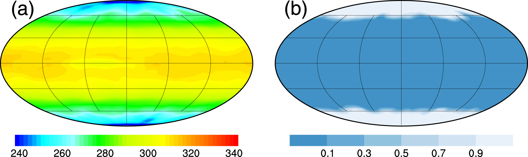
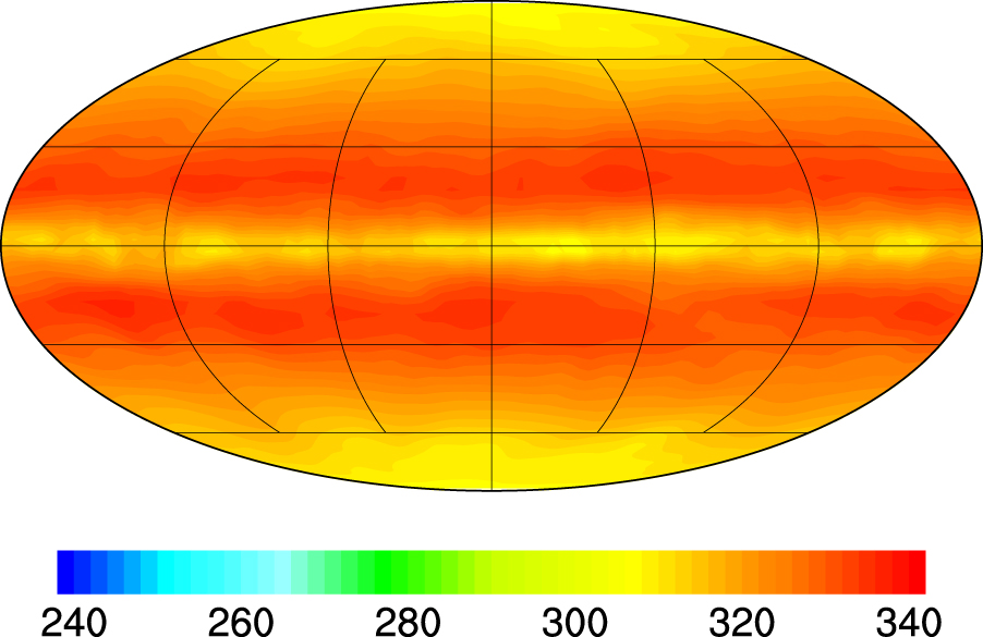
Figure 2(a) shows SATs in the L-CO2 simulation. The global-mean SAT is about 285 K. It is about 8 K lower than that in the E-CO2 simulation and 3 K lower than that of present-day Earth. The extremely low CO2 concentration does not cause much decrease in tropical surface temperatures compared with that in E-CO2 simulation. The highest surface temperature in the tropics remains as high as 308 K. The lowest temperatures are about 230 K in both polar regions. For such an extremely low level of CO2, sea-ice edges only extend to about 45° in latitude in both hemispheres (Figure 2(b)). The sea-ice edges are far away from the critical latitude of runaway freezing in snowball Earth simulations (Yang et al. 2012a, 2012b), suggesting that runaway freezing cannot happen even if the CO2 concentration is extremely low. The largest ice thickness is about 24 m over both poles. The results here indicate that Kepler 452b can still remain habitable even if sea-floor silicate weathering can efficiently reduce atmospheric CO2 concentrations to extremely low levels.
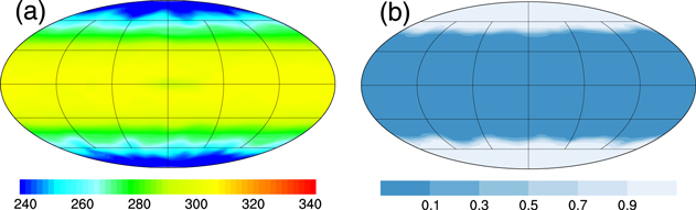
Figure 2. Global distributions of SATs and sea-ice fraction in the L-CO2 simulation. (a) SATs, units: K. (b) Sea-ice fraction, units: %.
Download figure:
Standard image High-resolution imageFor the H-CO2 simulation (Figure 3), the global-mean SAT is increased to 322 K. The highest SATs in the tropics are about 332 K. Note that the highest SATs are not located over the equator, but at about 15° north and south of the equator. This is because easterly winds over the tropics generate upwelling of cold water near the equator, and the Coriolis force drives warm surface water poleward. The lowest SATs in both polar regions are about 300 K, well above the freezing point of water. Thus, the planet becomes globally ice free as CO2 is increased to 0.2 bars. In the absence of silicate weathering, CO2 levels can accumulate to very high levels in the atmosphere throughout volcanic outgassing. Because the radiation transfer module in the present climate model can only remain accurate for CO2 levels no higher than 0.2 bars (Pierrehumbert 2005), we do not perform simulations for CO2 levels higher than 0.2 bars. For high levels of CO2, effects of pressure broadening of absorption lines of CO2 and water vapor as well as collision-induced CO2 absorption in the infrared region become important (Kasting et al. 1984; Kasting & Ackerman 1986). However, these radiative effects are not included in the climate model used here. However, from previous calculations using a radiation–convection model with these effects considered (Hu et al. 2011; Hu & Ding 2011), we know that the global-mean SAT can be increased by about 62 K as CO2 is increased from 0.2 bars (100000 ppmv) to 1.0 bar (400000 ppmv; see Figures 5 and 6 in Hu et al. 2011). Thus, the global-mean SAT can be above 380 K for 1 bar CO2. It suggests that Kepler 452b's global-mean SAT could be too hot to be habitable if there is no silicate weathering to limit CO2 concentrations in the atmosphere.
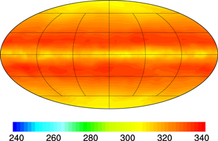
Figure 3. Global distribution of SATs in the H-CO2 simulation. Units: K.
Download figure:
Standard image High-resolution imageAnother great concern is whether Kepler 452b had lost all of its water because it has a much longer lifetime and is likely warmer than Earth. From the E-CO2 simulation, we have seen that the global-mean SAT is only 5 K higher than that of Earth. It suggests that for CO2 concentrations comparable to that in the Earth atmosphere the cold trapping region remains near the tropical tropopause, and that stratospheric water mixing ratios should have no dramatic increases. Thus, the diffusion-limited escape rate of water of Kepler 452b should not be very different from that of present-day Earth, and Kepler 452b's water inventory should be retained as long as the planet has a similar amount of water as that of Earth.
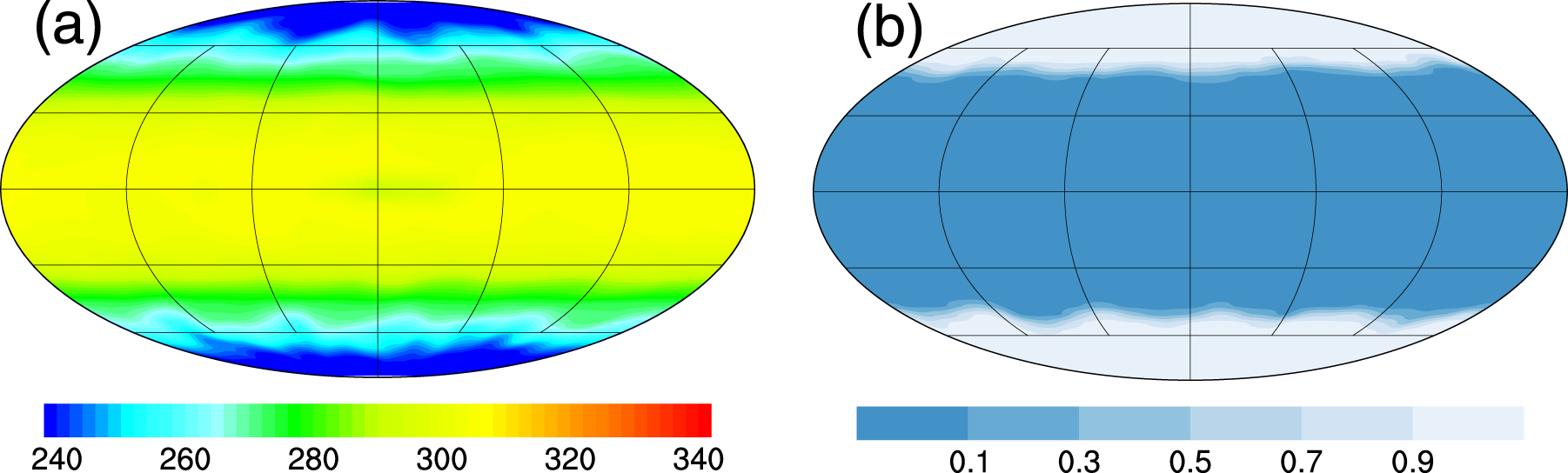
For the H-CO2 simulation, air temperatures are much higher than Earth's at all levels (Figure 4(a)), except for stratospheric polar regions where temperatures are as low as 150 K. At the tropical 100 hPa pressure level where the cold trapping region is located in the present Earth atmosphere, air temperatures are about 270 K. It suggests that water vapor can be readily transported to atmospheric layers above 100 hPa, without experiencing dehydration. As a consequence of such warm air temperatures, water vapor volume mixing ratios in the H-CO2 simulation are also much higher than that in the present Earth atmosphere (Figure 4(b)). Near the tropical surface, the water vapor volume mixing ratio is greater than 10%, about 1 order of magnitude higher than that on the present Earth. At 100 and 10 hPa, the maximum water vapor mixing ratios are about 10−2 and 10−3, respectively. These values are all about 3 orders of magnitude higher than that at the same levels of the present Earth atmosphere. As water molecules reach levels above 10 hPa, they are exposed to destructive ultraviolet stellar radiation and are photolyzed. Then, hydrogen would escape to space through diffusion processes. Note that high-level CO2, such as that in the H-CO2 simulation, generates strong cooling effects and thus low temperatures in the middle and upper atmospheres, although it greatly warms the surface and the troposphere. It is because CO2 emits IR radiation to space in the middle and upper atmosphere. Sufficiently low temperatures in the middle and upper atmosphere, which are beyond the model top here (one can see the cold temperatures in polar regions in Figure 4(a)), limit water vapor mixing ratios in the middle and upper atmosphere, and thus reduce the escape rate of hydrogen (Wordsworth & Pierrehumbert 2013a), and reduce the rate of water loss.

Figure 4. Vertical distributions of zonal-mean atmospheric temperatures and water vapor volume mixing ratio in the H-CO2 simulation. (a) Atmospheric temperatures, units: K. (b) Water vapor volume mixing ratio, units: part per volume.
Download figure:
Standard image High-resolution image
Here, we take the water mixing ratio to estimate the upper limit of the timescale of water loss. For an ocean with the depth of 4 km, as we assumed above, the column water molecule density would be 12.8 × 1027 cm−2. The diffusion-limited escape rate of water can be written as Φ H2O ≅ 2.5 × 10¹³ f(H2O) (Walker et al. 1981; Lissauer 1999; Selsis et al. 2007), where f(H2O) is the volume mixing ratio of water vapor. For the water vapor volume mixing ratio at 10 hPa (10−3), the diffusion-limited escape rate of water is about 2.5 × 1010 cm−2 s−1. Then, the upper limit of the timescale of total ocean water loss to space is about 16 billion years. It is much longer than Kepler 452b's lifetime of about 6.0 billion years. Therefore, water loss due to diffusion-limited escape processes may not seriously threaten Kepler 452b's habitability as long as the planet initially had an ocean with the same depth as Earth's.
There are other factors that would also extend the lifetime of ocean water. Although the total luminosity of Sun-like stars increases with stellar age, X-ray and extreme ultraviolet radiation decrease with time (Ribas et al. 2005). Thus, Kepler 452b should have a weaker rate of water photolysis for the same water vapor mixing ratio as present Earth's. In addition, water outgassing from the mantle reservoir can compensate for surface water loss and extend the time of water existence on Kepler 452b.
4. Discussion and Conclusions
Our simulation results demonstrate that Kepler 452b is a habitable exoplanet if its atmospheric CO2 concentrations are comparable or lower than that in the Earth atmosphere. The simulations also show that even for global-mean SAT as high as 322 K, Kepler 452b can still retain its water inventory if it initially had oceans with depths comparable to Earth's. However, if there is the lack of carbonate–silicate weathering to limit atmospheric CO2 concentration, Kepler 452b could become too hot to be habitable. If Kepler 452b is a partially ocean-covered planet (Cowan & Abbot 2014), CO2 concentration is limited by carbonate–silicate weathering over continents, and the planet should be habitable. If Kepler 452b is an aquaplanet, its habitability is determined by the efficiency of sea-floor weathering.
Super-Earth exoplanets, such as Kepler 452b, may have a denser atmosphere envelope than Earth's, with high-level nitrogen (N2) and hydrogen (H2). The radiative effects of these atmospheric compositions also have important impacts on Kepler 452b's climate. On the one hand, higher levels of N2 tend to stabilize the planet's climate by increasing Rayleigh scattering of stellar radiation and thus increasing the planet's planetary albedo (Kopparapu et al. 2014). On the other hand, the planet could be significantly warmed by H2–N2 collision-induced absorption of IR radiation (Wordsworth & Pierrehumbert 2013b), and high-level N2 will increase the pressure broadening of CO2, which leads to a greater greenhouse effect. These radiative effects are beyond the capability of the present model and thus are not studied here.
This study is supported by the National Natural Science Foundation of China under grants 41375072 and 41530423. We thank F. Ding for discussion.