


Abstract
We present the "SINS/zC-SINF AO survey" of 35 star-forming galaxies, the largest sample with deep adaptive optics (AO)–assisted near-infrared integral field spectroscopy at z ∼ 2. The observations, taken with SINFONI at the Very Large Telescope, resolve the Hα and [N ii] emission and kinematics on scales of ∼1.5 kpc. The sample probes the massive (M⋆ ∼ 2 × 10⁹ − 3 × 10¹¹ M⊙), actively star-forming (SFR ∼ 10–600 M⊙ yr−1) part of the z ∼ 2 galaxy population over a wide range of colors ((U − V)rest ∼ 0.15–1.5 mag) and half-light radii (Re,H ∼ 1–8.5 kpc). The sample overlaps largely with the "main sequence" of star-forming galaxies in the same redshift range to a similar KAB = 23 mag limit; it has ∼0.3 dex higher median specific SFR, ∼0.1 mag bluer median (U − V)rest color, and ∼10% larger median rest-optical size. We describe the observations, data reduction, and extraction of basic flux and kinematic properties. With typically 3–4 times higher resolution and 4–5 times longer integrations (up to 23 hr) than the seeing-limited data sets of the same objects, the AO data reveal much more detail in morphology and kinematics. The complete AO observations confirm the majority of kinematically classified disks and the typically elevated disk velocity dispersions previously reported based on subsets of the data. We derive typically flat or slightly negative radial [N ii]/ gradients, with no significant trend with global galaxy properties, kinematic nature, or the presence of an AGN. Azimuthal variations in [N ii]/
 are seen in several sources and are associated with ionized gas outflows and possibly more metal-poor star-forming clumps or small companions. The reduced AO data are made publicly available (http://www.mpe.mpg.de/ir/SINS/SINS-zcSINF-data).
Export citation and abstract BibTeX RIS
1. Introduction
The advent of high-throughput near-infrared (near-IR) integral field unit (IFU) spectrometers mounted on 8–10 m class telescopes in the past 15 yr has made it possible to spatially resolve the kinematics and distribution of the warm ionized gas in galaxies at redshift z ≳ 1. Near-IR IFU surveys have been instrumental in revealing that a significant proportion (≳50%) of massive z ∼ 1–3 star-forming galaxies (SFGs) are disks, characterized by high intrinsic local velocity dispersions of σ0 ∼ 25–100 km s−1 and typically irregular, often clumpy emission-line morphologies (e.g., Buitrago et al. 2014; Cresci et al. 2009; Épinat et al. 2009, 2012; Förster Schreiber et al. 2006, 2009; Genzel et al. 2006, 2008; Gnerucci et al. 2011a, 2011b; Jones et al. 2010b; Law et al. 2009; Leethochawalit et al. 2016; Mancini et al. 2011, hereafter M11; Molina et al. 2017; Newman et al. 2013; Shapiro et al. 2008; Stott et al. 2014, 2016; Swinbank et al. 2012a, 2012b; Wisnioski et al. 2011, 2012, 2015; Wright et al. 2009). High-resolution rest-UV/optical and Hα imaging of large mass-selected samples out to  obtained with the Hubble Space Telescope (HST) confirmed the prevalence of disklike morphologies among massive SFGs, with an increasingly important central stellar bulge-like component at higher galaxy masses and clumpier appearances toward shorter wavelengths (e.g., Wuyts et al. 2011b, 2012, 2013; Nelson et al. 2013, 2016b; Lang et al. 2014; see also Elmegreen et al. 2007, 2009; Law et al. 2012a; Tacchella et al. 2015b, 2018). Mapping and kinematics of the cold molecular gas in star-forming disks via low-lying CO line emission also revealed clumpy distributions and elevated intrinsic local velocity dispersions, showing that these characteristics are not just a property of the ionized gas layer but of the entire interstellar medium (ISM; e.g., Daddi et al. 2010; Tacconi et al. 2010, 2013; Swinbank et al. 2011; Genzel et al. 2013; Übler et al. 2018). From surveys of CO line and cold dust continuum emission, it is now well established that z ∼ 1–3 SFGs have high gas mass fractions of ∼30%–50% (see Carilli & Walter 2013; Tacconi et al. 2013, 2018; Genzel et al. 2015; Scoville et al. 2016 and references therein).
A widely invoked theoretical framework to interpret these properties is that of gas-rich, turbulent disks in which kpc-scale clumps form through violent disk instabilities, and bulge formation takes place via efficient secular processes and inward clump migration on timescales ≲1 Gyr (e.g., Noguchi 1999; Immeli et al. 2004a, 2004b; Bournaud et al. 2007, 2008, 2014; Genzel et al. 2008; Dekel et al. 2009; Jones et al. 2010b; Cacciato et al. 2012; Ceverino et al. 2012; Genel et al. 2012; Hopkins et al. 2012; Dekel & Burkert 2014). Theory and numerical simulations indicate that telltale signatures of physical processes at play appear on scales of ∼1 kpc and ∼10–100 km s−1 or less. Both high resolution and high sensitivity are needed to separate different components from each other in space and velocity, such as bulges and clumps in disks, perturbations induced by mergers, disk clumps or bar streaming, and narrow line profiles tracing the potential well versus broader components associated with gas outflows.
Most of the near-IR IFU data at z ∼ 1–3 published to date comprise seeing-limited observations. Good near-IR seeing conditions of ∼0 5 correspond to a spatial resolution of ∼4 kpc at z = 1–3. Observations aided by adaptive optics (AO) typically reach 3–4 times higher resolution or ∼1 kpc (and even better in the source plane for rare, strongly lensed sources). An important practical limitation for AO-assisted near-IR IFU observations is that targets must have both (1) an accurate redshift to ensure the lines of interest fall within atmospheric windows and away from the numerous bright night-sky lines in the near-IR and (2) a sufficiently bright nearby star providing a reference signal for the AO correction. Adding to the challenge, observing conditions must be favorable (good seeing, long atmospheric turbulence coherence time) to achieve significant image quality improvement with AO, and long integration times are required for faint distant galaxies. As a consequence, z ∼ 1–3 near-IR IFU AO samples are typically small and form a rather heterogeneous collection, and few objects benefit from very sensitive data.
Using SINFONI at the ESO Very Large Telescope (VLT), we carried out a substantial effort to collect a sizable sample of 35 typical massive z ∼ 2 SFGs with deep AO observations. The largest part of the data was obtained through an ESO Large Program (LP) and a small pilot program, building on two previous major programs: the "SINS" survey of z ∼ 1.5–3 galaxies with SINFONI and the "zCOSMOS" optical spectroscopic survey of 0 < z < 3 galaxies. The SINS survey observed a total of 80 galaxies, mostly in seeing-limited mode, and provided the first and largest near-IR IFU sample at z ∼ 2 at the time (Förster Schreiber et al. 2009, hereafter FS09). The galaxies were drawn from spectroscopically confirmed subsets of various samples selected by diverse photometric criteria. While three-quarters of the sources have a suitable AO reference star, routine AO operations with SINFONI began roughly midway into the 5 yr spanned by the SINS survey observing campaigns, so that only a handful of targets were initially followed up with AO. To expand and improve on the initial SINFONI+AO sample, we collected an additional 30 z ∼ 2 sources from the "zCOSMOS-deep" spectroscopic survey, which spans 1.4 < z < 3 and was conducted with VIMOS at the VLT (Lilly et al. 2007, 2009). This "zC-SINF" sample was selected with uniform criteria and such that all objects had an AO reference star and accurate spectroscopic redshift (M11), capitalizing on the wide area (the central ∼1 deg2 of the COSMOS field) and high sampling rate (∼50% to BAB = 25 mag) of the zCOSMOS-Deep survey (Diener et al. 2013).
Taken together, the SINS and zC-SINF samples comprise a total of 110 massive z ∼ 1–3 SFGs with seeing-limited SINFONI data, 35 of which were followed up with sensitive, high-resolution AO-assisted observations targeting the Hα and [N ii] emission lines. After the initial no-AO observations of the 30 new zC-SINF objects, the major part of our SINFONI LP (and its pilot program) was devoted to the AO observations of 26 targets. The AO data of a further nine SINS targets were obtained as part of complementary SINFONI+AO normal, open-time programs. The underlying strategy for all these programs was ultimately to collect high-quality AO data for a reliable overview of kpc-scale kinematics and emission-line properties over a wide range in stellar mass (M⋆) and star formation rate (SFR) and to obtain very deep AO data of a subset most suitable to investigate particular dynamical/physical processes.
This strategy was motivated by a specific set of science goals: (1) to quantify the fraction and structure of disks and mergers, (2) to investigate what dynamical processes drive the early evolution of galaxies, (3) to determine the origin of the large turbulence in high-z disks, (4) to constrain the relative importance of gas accretion and mass and metals redistribution, (5) to map the strength of galactic winds on galactic and subgalactic (clump) scales and investigate the mechanisms and energetics of feedback from star formation and active galactic nuclei (AGNs), (6) to unveil the nature of compact dispersion-dominated objects, and (7) to shed light on the relative growth of bulges and supermassive black holes. The SINS/zC-SINF project motivated three dedicated HST imaging follow-up programs (Förster Schreiber et al. 2011a; Tacchella et al. 2015b, 2018) to map the stellar light at a resolution comparable to that of the SINFONI+AO data, enhancing the exploitation of the line emission and kinematics data.
Over the 12 yr during which the SINFONI+AO data were taken, key science results addressing the goals listed above based on a subset of targets and/or the observations were published in several papers, which we summarize here.
- 1.Our first and deepest AO-assisted observations of a z ∼ 2 galaxy to date revealed for the first time the prototypical properties of massive high-redshift SFGs: a large rotating disk with elevated intrinsic gas velocity dispersion, several distinct star-forming clumps, and evidence for a powerful gas outflow driven by AGN activity (Genzel et al. 2006, 2008, 2011, 2014a; Förster Schreiber et al. 2014).
- 2.
- 3.
- 4.The detection and characterization of the physical properties of the ubiquitous star formation- and AGN-driven winds in typical z ∼ 2 massive SFGs on galactic and subgalactic scales—as diagnosed by the Hα+[N ii] (+[S ii]) line profiles—was uniquely enabled by the sensitive SINFONI data (Shapiro et al. 2009; Genzel et al. 2011, 2014b; Newman et al. 2012a, 2012b; Förster Schreiber et al. 2014).
- 5.
- 6.
We present here the complete sample of 35 SINS/zC-SINF objects with SINFONI+AO observations, the survey strategy, and the characteristics of the data sets. The paper is organized as follows. We describe the selection and global properties of the sample in Section 2, the observations and data reduction in Section 3, and the extraction of maps and spectra in Section 4. We present the measurements of Hα sizes and global surface brightness distributions in Section 5 and the kinematic properties in Section 6. In Section 7, we revisit the nature of the galaxies (i.e., disks versus nondisks) based on their kinematics and morphologies, and in Section 8, we exploit the AO data to constrain spatial variations in [N ii]/ ratio. The paper is summarized in Section 9. Several technical aspects of the AO observations and data analysis can be found in the appendices, including the presentation of the full data set and a comparison of the results obtained from the SINFONI AO and no-AO data. Throughout, we assume a Λ-dominated cosmology with H0 = 70 h70 km s−1 Mpc−1, Ωm = 0.3, and ΩΛ = 0.7. For this cosmology, 1'' corresponds to 8.3 kpc at z = 2.2. Magnitudes are given in the AB photometric system unless otherwise specified.
2. SINS/zC-SINF AO Sample
The SINFONI AO targets form a subset of the SINS and zC-SINF Hα samples at  initially observed in natural seeing. Table 1 lists the galaxies of the AO sample, their Hα redshifts, K-band magnitudes, and several other global properties. An exhaustive description of the selection of the parent sample and the derivation of stellar properties is given by FS09 and M11 (with updated results for six objects using new H-band photometry presented by Förster Schreiber et al. 2011a). We refer the reader to these papers for details and highlight the salient points in this section.
Table 1. SINS/zC-SINF AO Survey: Sample Galaxies
| Source | R.A. | Decl. | KABa | zHαb | M⋆ | AV | SFRSED | sSFRSED | SFRUV+IRc | sSFRUV+IR | (U − V)restd | Notese |
|---|---|---|---|---|---|---|---|---|---|---|---|---|
| (mag) | (1010 M⊙) | (mag) | (M⊙ yr−1) | (Gyr−1) | (M⊙ yr−1) | (Gyr−1) | (mag) | |||||
| Q1623-BX455 | 16:25:51.7 | +26:46:55 | 23.41 | 2.4078 | 1.03 | 0.6 | 15 | 1.5 | ⋯ | ⋯ | 0.67 | ⋯ |
| Q1623-BX502 | 16:25:54.4 | +26:44:09 | 23.89 | 2.1557 | 0.23 | 0.4 | 14 | 6.0 | ⋯ | ⋯ | 0.14 | ⋯ |
| Q1623-BX543 | 16:25:57.7 | +26:50:09 | 22.39 | 2.5209 | 0.94 | 0.8 | 145 | 15.5 | ⋯ | ⋯ | 0.24 | ⋯ |
| Q1623-BX599 | 16:26:02.6 | +26:45:32 | 21.78 | 2.3312 | 5.66 | 0.4 | 34 | 0.6 | ⋯ | ⋯ | 0.93 | ⋯ |
| Q2343-BX389 | 23:46:28.9 | +12:47:34 | 22.04 | 2.1724 | 4.12 | 1.0 | 25 | 0.6 | ⋯ | ⋯ | 1.29 | ⋯ |
| Q2343-BX513 | 23:46:11.1 | +12:48:32 | 21.95 | 2.1082 | 2.70 | 0.2 | 10 | 0.4 | ⋯ | ⋯ | 0.93 | ⋯ |
| Q2343-BX610 | 23:46:09.4 | +12:49:19 | 21.07 | 2.2107 | 10.0 | 0.8 | 60 | 0.6 | ⋯ | ⋯ | 0.93 | 1 |
| Q2346-BX482 | 23:48:13.0 | +00:25:46 | (22.34)f | 2.2571 | 1.84 | 0.8 | 80 | 4.3 | ⋯ | ⋯ | 0.77 | ⋯ |
| Deep3a-6004 | 11:25:03.8 | −21:45:33 | 20.79 | 2.3871 | 31.6 | 1.8 | 214 | 0.7 | 355 | 1.1 | 1.52 | 1 |
| Deep3a-6397 | 11:25:10.5 | −21:45:06 | 19.96 | 1.5133 | 12.0 | 2.2 | 563 | 4.7 | 214 | 1.8 | 1.28 | 1 |
| Deep3a-15504 | 11:24:15.6 | −21:39:31 | 21.03 | 2.3830 | 10.9 | 1.0 | 150 | 1.4 | 146 | 1.3 | 0.71 | 1 |
| K20-ID6 | 03:32:29.1 | −27:45:21 | 22.13 | 2.2348 | 2.67 | 1.0 | 45 | 1.7 | 47 | 1.8 | 0.91 | ⋯ |
| K20-ID7 | 03:32:29.1 | −27:46:29 | 21.47 | 2.2240 | 3.95 | 1.0 | 112 | 2.8 | 101 | 2.6 | 0.49 | ⋯ |
| GMASS-2303 | 03:32:38.9 | −27:43:22 | 22.78 | 2.4507 | 0.72 | 0.4 | 21 | 2.9 | IR-undet | IR-undet | 0.46 | ⋯ |
| GMASS-2363 | 03:32:39.4 | −27:42:36 | 22.67 | 2.4520 | 2.16 | 1.2 | 64 | 2.9 | 45 | 2.1 | 0.87 | ⋯ |
| GMASS-2540 | 03:32:30.3 | −27:42:40 | 21.80 | 1.6146 | 1.89 | 0.6 | 21 | 1.1 | 32 | 1.7 | 0.96 | ⋯ |
| SA12-6339 | 12:05:32.7 | −07:23:38 | 22.00 | 2.2971 | 2.57 | 2.0 | 620 | 24 | ⋯ | ⋯ | 0.61 | ⋯ |
| ZC400528 | 09:59:47.6 | +01:44:19 | 21.08 | 2.3873 | 11.0 | 0.9 | 148 | 1.3 | 556 | 5.1 | 0.84 | 1 |
| ZC400569 | 10:01:08.7 | +01:44:28 | 20.69 | 2.2405 | 16.1 | 1.4 | 241 | 1.5 | 239 | 1.5 | 1.29 | 1,2 |
| ZC400569N | 10:01:08.7 | +01:44:28 | ⋯ | 2.2432 | 12.9 | ⋯ | 157 | 1.2 | 156 | 1.2 | ⋯ | 1,2 |
| ZC401925 | 10:01:01.7 | +01:48:38 | 22.74 | 2.1413 | 0.58 | 0.7 | 47 | 8.2 | IR-undet | IR-undet | 0.40 | ⋯ |
| ZC403741 | 10:00:18.4 | +01:55:08 | 21.02 | 1.4457 | 4.45 | 1.6 | 113 | 2.5 | IR-undet | IR-undet | 0.99 | ⋯ |
| ZC404221 | 10:01:41.3 | +01:56:43 | 22.44 | 2.2199 | 1.57 | 0.7 | 61 | 3.9 | IR-undet | IR-undet | 0.40 | ⋯ |
| ZC405226 | 10:02:19.5 | +02:00:18 | 22.33 | 2.2870 | 0.93 | 1.0 | 117 | 12.6 | IR-undet | IR-undet | 0.56 | ⋯ |
| ZC405501 | 09:59:53.7 | +02:01:09 | 22.25 | 2.1539 | 0.84 | 0.9 | 85 | 10.1 | IR-undet | IR-undet | 0.33 | ⋯ |
| ZC406690 | 09:58:59.1 | +02:05:04 | 20.81 | 2.1950 | 4.14 | 0.7 | 200 | 4.8 | 296 | 7.2 | 0.56 | ⋯ |
| ZC407302 | 09:59:56.0 | +02:06:51 | 21.48 | 2.1819 | 2.44 | 1.3 | 340 | 13.9 | 358 | 14.7 | 0.50 | ⋯ |
| ZC407376 | 10:00:45.1 | +02:07:05 | 21.79 | 2.1729 | 2.53 | 1.2 | 89 | 3.5 | 124 | 4.9 | 0.80 | 3 |
| ZC407376S | 10:00:45.1 | +02:07:05 | ⋯ | 2.1730 | 1.39 | ⋯ | 67 | 4.8 | 93 | 6.7 | ⋯ | 3 |
| ZC407376N | 10:00:45.2 | +02:07:06 | ⋯ | 2.1728 | 1.14 | ⋯ | 22 | 1.9 | 31 | 2.7 | ⋯ | 3 |
| ZC409985 | 09:59:14.2 | +02:15:47 | 22.30 | 2.4569 | 1.61 | 0.6 | 51 | 3.2 | IR-undet | IR-undet | 0.64 | ⋯ |
| ZC410041 | 10:00:44.3 | +02:15:59 | 23.16 | 2.4541 | 0.46 | 0.6 | 47 | 10.2 | IR-undet | IR-undet | 0.36 | ⋯ |
| ZC410123 | 10:02:06.5 | +02:16:16 | 22.80 | 2.1986 | 0.42 | 0.8 | 59 | 13.9 | IR-undet | IR-undet | 0.31 | ⋯ |
| ZC411737 | 10:00:32.4 | +02:21:21 | 22.81 | 2.4442 | 0.34 | 0.6 | 48 | 13.9 | IR-undet | IR-undet | 0.53 | ⋯ |
| ZC412369 | 10:01:46.9 | +02:23:25 | 21.39 | 2.0281 | 2.17 | 1.0 | 94 | 4.3 | IR-undet | IR-undet | 0.88 | ⋯ |
| ZC413507 | 10:00:24.2 | +02:27:41 | 22.52 | 2.4800 | 0.88 | 1.1 | 111 | 12.6 | IR-undet | IR-undet | 0.57 | ⋯ |
| ZC413597 | 09:59:36.4 | +02:27:59 | 22.58 | 2.4502 | 0.75 | 1.0 | 84 | 11.3 | IR-undet | IR-undet | 0.51 | ⋯ |
| ZC415876 | 10:00:09.4 | +02:36:58 | 22.38 | 2.4354 | 0.92 | 1.0 | 94 | 10.2 | IR-undet | IR-undet | 0.68 | ⋯ |
Notes. The stellar properties are taken from Förster Schreiber et al. (2009, 2011a) and M11 and were derived using Bruzual & Charlot (2003) models with a Chabrier (2003) IMF, solar metallicity, the Calzetti et al. (2000) reddening law, and either constant or exponentially declining SFRs (see text). Stellar masses correspond to those in live stars and remnants. Uncertainties for the stellar properties derived from SEDs are dominated by systematics from model assumptions; for this sample and the analyses throughout this paper, we adopt typical uncertainties of 0.2 dex in  , 0.3 mag in AV, and 0.47 dex in
  .
.
 .
dRest-frame U − V colors derived following the procedure described by Wuyts et al. (2012; see also Taylor et al. 2009; Brammer et al. 2011). Uncertainties are dominated by those of the observed photometry and systematics from the set of templates used for interpolation and are typically estimated to be 0.1 mag.
e(1) These objects have evidence for an AGN (Section 2.2). (2) ZC400569 has a complex morphology characterized by a brighter northern source and a southern clumpy extension; the stellar mass and SFR of the dominant northern component are scaled from the total values according to the fractions estimated from the stellar mass map (based on HST/WFC3 near-IR imaging) and the observed Hα line map, respectively. (3) ZC407376 is an interacting pair; the stellar mass and SFR of each component are scaled from those of the total system according to the fractions estimated from the HST/WFC3-based stellar mass map and the observed Hα line map, respectively.
fFor Q2346-BX482, no K-band photometry is available; here we give the H-band magnitude from HST/NICMOS imaging through the F160W filter (Förster Schreiber et al. 2011a).
.
dRest-frame U − V colors derived following the procedure described by Wuyts et al. (2012; see also Taylor et al. 2009; Brammer et al. 2011). Uncertainties are dominated by those of the observed photometry and systematics from the set of templates used for interpolation and are typically estimated to be 0.1 mag.
e(1) These objects have evidence for an AGN (Section 2.2). (2) ZC400569 has a complex morphology characterized by a brighter northern source and a southern clumpy extension; the stellar mass and SFR of the dominant northern component are scaled from the total values according to the fractions estimated from the stellar mass map (based on HST/WFC3 near-IR imaging) and the observed Hα line map, respectively. (3) ZC407376 is an interacting pair; the stellar mass and SFR of each component are scaled from those of the total system according to the fractions estimated from the HST/WFC3-based stellar mass map and the observed Hα line map, respectively.
fFor Q2346-BX482, no K-band photometry is available; here we give the H-band magnitude from HST/NICMOS imaging through the F160W filter (Förster Schreiber et al. 2011a).
Download table as: ASCIITypeset image
The stellar mass, visual extinction (AV), and SFR (SFRSED) of the galaxies were derived from evolutionary synthesis modeling of their optical to near-IR broadband spectral energy distributions (SEDs) supplemented with mid-IR 3–8 μm photometry when available. Model assumptions dominate the uncertainties of the derived stellar properties. In general, however, for observed SEDs covering up to at least near-IR wavelengths, and for similar model evolutionary tracks and star formation histories, the relative ranking of galaxies in these properties is fairly robust (e.g., Förster Schreiber et al. 2004; Shapley et al. 2005; Wuyts et al. 2007, 2011a; Maraston et al. 2010; M11). For consistency, we adopted best-fit results for the SINS and zC-SINF samples obtained with the same Bruzual & Charlot (2003) code, a Chabrier (2003) IMF, solar metallicity, the Calzetti et al. (2000) reddening law, and constant or exponentially declining SFRs.28
Table 1 also lists the rest-frame U − V color of the galaxies and, for objects in fields with mid- or far-IR coverage with the Spitzer/MIPS or Herschel/PACS instruments (COSMOS, GOODS-South, and Deep3a) and detected in at least one of the 24, 70, 100, or 160 μm bands, the SFR from the emergent rest-UV and IR emission (SFRUV+IR). The rest-frame photometry was computed from interpolation of the observed photometry using the code EAZY (Brammer et al. 2008). The SFRUV+IR estimates were derived following the prescriptions of Wuyts et al. (2011a): the UV contribution was calculated from the rest-frame 2800 Å luminosity, and the IR contribution was derived from the longest wavelength at which an object is detected.29 Throughout the paper, we use the SFRUV+IR when available and the SFRSED otherwise.
The SINS/zC-SINF AO sample includes six galaxies with evidence for a Type 2 AGN, noted in Table 1. Two of them were known to host an AGN based on the detection of rest-UV spectral signatures and a 1.4 GHz radio emission excess (Genzel et al. 2006; Förster Schreiber et al. 2014). As discussed by Förster Schreiber et al. (2014; see also Newman et al. 2014), the high-resolution SINFONI+AO  [N ii] data, supplemented with seeing-limited maps of [O iii] and Hβ obtained for four objects, further indicate the presence of an AGN through the line ratios and high-velocity gas outflow signatures in the central few kpc of all of the AO targets more massive than
  , including four cases previously unidentified as hosting an AGN.
2.1. Selection of the Parent SINS/zC-SINF Seeing-limited Sample
The SINS Hα targets were drawn from large optical spectroscopic surveys of  candidates selected by their
  optical colors ("BX/BM" objects; Steidel et al. 2004), K-band magnitudes (the "K20" survey at
  , Cimatti et al. 2002; the Gemini Deep Deep Survey (GDDS) at
  , Abraham et al. 2004), 4.5 μm magnitudes (the Galaxy Mass Assembly ultra-deep Spectroscopic Survey (GMASS) at
  , Cimatti et al. 2008; Kurk et al. 2013), or a combination of K-band and BzK color criteria (from the survey by Kong et al. 2006 of the "Deep3a" field of the ESO Imaging Survey; Renzini & Da Costa 1997). The SINS BX/BM targets were more specifically taken from the near-IR long-slit spectroscopic follow-up with NIRSPEC at the Keck II telescope of Erb et al. (2006b), and the SINS K20 objects comprised all five z > 2 sources discussed by Daddi et al. (2004). In addition to a reliable optical redshift, the selection criteria common to all SINS targets were that Hα falls in wavelength intervals of high atmospheric transmission and away from bright night-sky lines, object visibility during the observing runs, and an observed integrated line flux of ≳5 × 10⁻¹⁷ erg s−1 cm−2 in existing long-slit spectroscopy (for the BX/BM objects) or expected based on the best-fit SFRSED and AV values. Fainter sources were discarded because of prohibitively long integration times for detection, but we note that this criterion, applied last in the selection, removed very few objects. As argued by FS09, the diversity of criteria employed for the surveys from which the SINS targets were drawn makes the resulting sample less biased than any of its constituent subsamples.
The zC-SINF sample was drawn from the spectroscopic zCOSMOS-Deep survey carried out with VLT/VIMOS (Lilly et al. 2007, 2009), covering the central 1 deg2 of the 2 deg2 COSMOS field (Scoville et al. 2007). Reliable optical redshifts (zopt) were derived for ∼6000 objects at 1.4 < z < 2.5, preselected at  and according to the BzK or BX/BM color criteria. The zC-SINF SINFONI targets were then culled among those within 30'' of a
  star enabling natural guide star (NGS) AO (with one exception), a sufficiently secure redshift, avoidance of spectral regions with bright night-sky lines and/or low atmospheric transmission for the Hα line, and a minimum SFR of ∼ 10 M⊙ yr−1 (see M11 for details). This SFR roughly matches the minimum Hα flux criterion for the SINS galaxies at z = 2 assuming AV = 1 mag, and, as for the SINS sample, this cut removes only a few objects. Of the 62 viable SINFONI targets thus culled, the best 30 in terms of all criteria combined were observed. Of this zC-SINF sample, 29 belong to the zCOSMOS-Deep subset preselected with the BzK criteria, and one is from the "BX" subset.
The resulting SINS and zC-SINF Hα seeing-limited samples range in redshift from 1.35 to 2.58, with median z = 2.22; 76% of the targets are at z > 2. The fraction of objects with Hα detected in the seeing-limited data is 84%. Although non-AGN targets were preferentially selected, six of the galaxies observed were known to host an AGN based on diagnostic features in their rest-UV spectra, their strong mid-IR excess, or their brightness in X-ray or radio emission depending on the multiwavelength and spectroscopic coverage of the sources in different fields. As noted above, our SINFONI data added four cases with evidence for an AGN from their rest-optical emission-line properties. The different diagnostics available among the fields prevent a reliable assessment of AGN fraction and biases with respect to this population for the SINS/zC-SINF sample. The increase in AGN fraction with higher galaxy mass is, however, fully consistent with the trends observed from much larger multiwavelength and spectroscopic surveys at z ∼ 2 (e.g., Reddy et al. 2005; Daddi et al. 2007; Brusa et al. 2009; Bongiorno et al. 2012; Hainline et al. 2012; Mancini et al. 2015).
2.2. Selection of the SINS/zC-SINF AO Sample
For the SINFONI+AO observations, 17 targets were taken from the parent SINS seeing-limited survey and 18 from the zC-SINF sample. They were mostly chosen to lie at z > 2, although three objects at z ∼ 1.5 were considered. The redshifts range from 1.45 to 2.52, with a median z = 2.24, approximately the same as for the parent seeing-limited sample. The goal of the SINFONI LP was to collect AO data of ∼25 sources covering the  plane as widely as possible and obtain a set of "benchmark objects" to relate resolved kinematics, star formation, and physical conditions with global properties of the massive SFG population. Some of the objects had been previously observed with AO as part of other programs; for them, the additional LP observations aimed at a substantial increase in the sensitivity of the data sets. In addition to the final 26 AO targets of the LP, nine other galaxies were observed during the course of various SINFONI+AO programs addressing more specific, though related, science goals. The total number of targets results from the trade-off between sample size and S/N of the data within the constraints set by the available observing time.
The SINS objects were taken among those with a suitable AO reference star ( and distance from the galaxy <60''), except for one without a nearby bright star that was observed in the so-called "Seeing Enhancer" (SE) mode (see Section 3.1). Some preference was given to brighter SINS objects with a source-integrated Hα flux ≳10−16 erg s−1 cm−2, although three fainter sources were included (GMASS-2303, GMASS-2363, and K20-ID6, with fluxes of (3–5) × 10−17 erg s−1 cm−2). In general, for these SINS AO targets, emphasis was given to larger disklike systems or compact objects with velocity dispersion–dominated kinematics in seeing-limited data. One object identified as a merger from seeing-limited kinematics (K20-ID7; see Shapiro et al. 2008) was also observed. These choices were driven by the aim of obtaining very deep kpc-scale-resolution IFU data of objects in different kinematic classes, unveiling the nature of the most compact sources, and studying in detail the dynamical and star formation processes in early disks (see Genzel et al. 2006, 2008, 2011, 2014a; Newman et al. 2012b, 2013).
The choice of zC-SINF objects for the AO observations was more objective and dictated by the targets being detected in the 1–2 hr natural seeing observations and the goal of ensuring wide  coverage in combination with the SINS AO targets. No explicit Hα flux or S/N cut was applied for the zC-SINF AO targets; their integrated Hα fluxes are in the range ∼4 × 10⁻¹⁷–6 × 10⁻¹⁶ erg s−1 cm−2. The Hα morphology and kinematics were not considered, except to exclude two candidate Type 1 AGNs based on their bright and point-like morphologies in Hα and HST broadband imaging in conjunction with their X-ray emission and rest-UV spectral features. For both SINS and zC-SINF AO targets, no explicit requirement on the averaged Hα surface brightness was used; instead, the integration times were adjusted to optimize the S/N per resolution element.
2.3. Global Stellar and Color Properties of the Samples
In terms of stellar mass, SFR, and color, the SINS/zC-SINF AO sample is fairly representative of its parent seeing-limited sample. This is shown in Figure 1, which compares their distributions in M⋆ versus SFR and (U − V)rest color diagrams. To place the samples in a broader context, Figure 1 also shows the distributions of the underlying galaxy population in the COSMOS field at 1.4 < z < 2.6 to  —similar to the ranges for the SINS/zC-SINF objects. Since here we are primarily interested in massive SFGs, objects in the reference sample with a specific
  are excluded, where
  is the Hubble time at the redshift of each source. This cut removes a small fraction (17%) of all
  sources at 1.4 < z < 2.6 (and only 12% for the
  interval encompassing ≥80% of the parent SINS/zC-SINF sample and the AO subset). The stellar properties and colors for the reference sample are taken from Wuyts et al. (2011b), where they were computed using the source catalog of Ilbert et al. (2009) supplemented with Spitzer/MIPS and Herschel/PACS mid- and far-IR photometry (Le Floc'h et al. 2009; Berta et al. 2011; Lutz et al. 2011) in a similar fashion as for the SINS/zC-SINF objects. Because the reference SFG sample is magnitude-limited, it is dominated by galaxies toward lower redshifts (median z = 1.7) compared to the SINS/zC-SINF samples (median z = 2.2). The different redshift distributions are reflected in the small vertical shift between the peak in density distribution for the reference population and the M⋆ versus SFR and (U − V)rest relationships at z = 2.2 in Figure 1. To account for evolutionary effects, the inset in each panel shows the distributions in terms of offsets in specific SFR and color from the relationships at the redshift and mass of the individual galaxies (see below).

Figure 1. Distributions in stellar and color properties of the SINS/zC-SINF AO sample and the parent Hα sample observed with SINFONI in seeing-limited mode. The SINFONI samples are compared to 1.4 < z < 2.6 SFGs in the COSMOS field at Ks,AB < 23.0 mag and with inverse specific SFR lower than the Hubble time at the redshift of each object. The SINS/zC-SINF galaxies are plotted as large circles (z > 2) and squares (z < 2), with red symbols showing those observed with AO. The density distribution of COSMOS SFGs is shown in green, with contours corresponding to fractions of 0.1, 0.3, 0.5, 0.7, 0.9, and 0.98 of the maximum. The green filled, gray hatched, and red hatched histograms show the fractional distributions projected onto each axis for the reference SFG population and the SINFONI seeing-limited and AO samples, respectively (with median z of 1.73, 2.22, and 2.24). Left: stellar mass vs. SFR. The solid line indicates the MS of SFGs at z = 2.2 from Whitaker et al. (2014); dashed and dotted lines correspond to offsets in SFR relative to the MS, as labeled in the plot. The inset shows the distributions of the offsets in specific SFR (in logarithmic units) of the reference SFG sample and the SINS/zC-SINF no-AO and AO targets relative to the MS at the mass and redshift of each individual source. Right: stellar mass vs. rest-frame U − V color. The solid line indicates the mean (U − V)rest as a function of  of the reference SFG sample around z = 2.2 (see Section 2.3). The inset shows the distributions of the reference SFG, SINFONI no-AO, and AO samples in color offset from the M⋆ versus (U − V)rest relation accounting for its zero-point evolution (∝ −0.24 × z). The SINS/zC-SINF AO sample covers similar ranges in M⋆, SFR,
  , and (U − V)rest as the parent no-AO sample and somewhat emphasizes the bluer targets at fixed stellar mass. The SINS/zC-SINF objects have a similar coverage in M⋆ as the reference SFG sample but preferentially probe the more actively star-forming and bluer part of this population.
Download figure:
Standard image High-resolution imageThe SINS/zC-SINF AO and the parent seeing-limited samples cover nearly identical ranges in stellar mass and SFR ( , SFR ∼ 10–650 M⊙ yr−1). The median (mean) values in stellar mass and SFR are nearly the same, with
  (∼4 × 10¹⁰ M⊙) and SFR ∼ 80 M⊙ yr−1 (∼125 M⊙ yr−1). The (U − V)rest colors of the AO targets range from ∼0.15 to ∼1.5 mag, compared to
  to ∼2.1 mag for the full seeing-limited sample. The median and mean colors of the AO sample are 0.67 and 0.71 mag, slightly bluer than those for the parent no-AO sample (0.83 and 0.82, respectively). For comparison, the reference SFG sample has median values of M⋆ ∼ 1.5 × 10¹⁰ M⊙, SFR ∼ 30 M⊙ yr−1, and
  . The ranges in properties for the SINS/zC-SINF samples overlap largely with those of the more general z ∼ 2 SFG population. It is, however, apparent from Figure 1 that they probe preferentially higher specific SFRs and bluer colors at fixed stellar mass, as illustrated by the distributions in the inset of each panel and obtained as follows.
The trend in specific SFR can be quantified through the offset relative to the "main sequence" (MS) delineated by the distribution of SFGs in the  plane,
  . For this purpose, we used the MS parameterization of Whitaker et al. (2014) and calculated the offsets at the redshift and stellar mass of each individual object. The SINS/zC-SINF no-AO sample extends down to 0.7 dex below and up to 1.2 dex above the MS, with a median (mean) ∼0.35 dex (∼0.30 dex) above the MS. The
  distribution for the AO sample spans a similar range, from 0.7 dex below up to 1.0 dex above the MS, with a median (mean) offset of ∼0.35 dex (∼0.25 dex). About 75% of the SINS/zC-SINF seeing-limited and AO targets lie above the MS at their redshift and mass; several of them have an sSFR >4 times larger than the MS and would qualify as "starbursts" according to Rodighiero et al. (2011). The bias toward higher sSFRs is more important at lower M⋆ (a result of the target selection introducing an effective lower SFR limit of ∼10 M⊙ yr−1).
The trend in colors of the SINS/zC-SINF samples relative to the bulk of z ∼ 2 SFGs can be quantified in an analogous manner. At fixed stellar mass and redshift, the distribution of the reference SFG sample is well approximated by a Gaussian. The mean (U − V)rest color from Gaussian fits in stellar mass bins within a redshift slice30
increases as a function of  with approximately constant slope. We thus defined the locus of SFGs in
  space by fitting a line to these values, with the evolution over z ∼ 1–3 being mostly in the zero point. The color offset relative to relationship at the mass and redshift of an object is denoted Δ(U − V)rest. The Δ(U − V)rest values of the SINS/zC-SINF seeing-limited sample span −0.6 to 0.9 mag, with a small median and mean offset of ∼−0.03 mag. The AO subset covers a narrower range of −0.55 to 0.25 mag, with median and mean offsets of ≈−0.10 mag. Accounting for the redshift and mass of the targets, about 65% of the no-AO sample lies on the blue side of the SFG locus in M⋆ versus (U − V)rest, and 70% of the AO targets do.
The preferentially higher sSFRs and bluer rest-optical colors of the SINS/zC-SINF samples compared to the underlying population of massive SFGs results from the combination of selection criteria, as extensively discussed by FS09 and M11. In particular, even for a primary selection at near-/mid-IR wavelengths (as for the majority of our targets), the mandatory zopt means in practice an optical magnitude cut to ensure sufficient S/N for a reliable redshift determination. This limit is typically ∼25–26 mag for the spectroscopic surveys from which the galaxies were drawn and implies that on average, the objects have bluer colors than an unbiased, purely K- (or mass-) selected sample in the same redshift range. In addition, the requirement of minimum Hα flux (or SFR) likely emphasizes younger, less obscured, and more actively star-forming systems, but we note again that few objects were discarded as SINFONI targets by this criterion, applied last in the selection process. An examination of the optical brightness and SFR distributions of photometrically selected candidate  galaxies and spectroscopically confirmed subsets in public data sets for popular deep fields (GOODS, COSMOS) confirms that biases toward higher sSFRs and bluer colors result largely from the optical magnitude limits of the spectroscopic surveys.
2.4. Rest-optical Size Distribution of the Samples
The strategies for both SINS and zC-SINF relied on the detection of Hα emission in 1–2 hr on-source integrations in natural seeing. Therefore, while no surface brightness criterion was applied, there is an implicit bias toward galaxies with at least some regions above a minimum Hα surface brightness. This effect could plausibly set the upper envelope in the Hα size versus flux distribution of the parent no-AO sample (FS09; M11), and, consequently, the AO sample may be missing the largest objects at any given integrated line flux. It is also possible that the most extended objects at a given optical magnitude are underrepresented because a low surface brightness may have prevented reliable redshift measurements. On the other hand, some of the more subjective choices made in particular for the AO follow-up of the SINS targets may have favored overall larger-than-average objects (see Section 2.2).
Figure 2 compares the distributions in M⋆ versus effective radius Re of our SINFONI samples to those of the underlying population of SFGs. We considered rest-frame optical continuum sizes obtained from H-band observations, less prone to the effects of extinction and localized star formation than the rest-UV or Hα. Here the reference SFG population is taken from the CANDELS/3D-HST surveys (Grogin et al. 2011; Koekemoer et al. 2011; Skelton et al. 2014; Momcheva et al. 2016), which provide the largest sample with sizes measured in the near-IR from HST imaging (van der Wel et al. 2012, 2014b). The same redshift, K magnitude, and sSFR cuts are applied as for the COSMOS reference sample in the previous subsection (the 3D-HST reference sample has similar median z = 1.8). The H-band sizes are available for 51 objects in our full SINS/zC-SINF sample and 29 of the AO targets; we use the measurements presented by Förster Schreiber et al. (2011a) and Tacchella et al. (2015b), as well as van der Wel et al. (2012), for the other objects that fall within the CANDELS/3D-HST fields.

Figure 2. Distribution in stellar mass vs. size of the SINS/zC-SINF AO sample and the parent Hα sample observed in seeing-limited mode. The SINFONI samples are compared to 1.4 < z < 2.6 SFGs in the CANDELS/3D-HST fields at Ks,AB < 23.0 mag and with inverse specific SFR lower than the Hubble time at the redshift of each object. Symbols and colors are the same as in Figure 1. In the main plot, the sizes are the major-axis effective radii derived from HST H-band imaging, available for 51 targets in the full SINS/zC-SINF sample and 29 targets from the AO subset. The solid and dashed lines indicate the mass–size relation for SFGs at z = 2.2 from van der Wel et al. (2014b) and the offsets by factors of two around it. The inset shows the distributions of the offsets in  from the mass–size relation at the mass and redshift of each individual source, where the sizes are corrected to a reference rest-frame wavelength of 5000 Å to account for the (small) effects of color gradients. The SINS/zC-SINF AO sample covers similar ranges in
  and
and  as the parent no-AO sample and the reference population of SFGs, with only a small shift toward larger sizes at fixed mass (by ∼10% on average).
Download figure:
Standard image High-resolution imageThe size distribution of the SINS/zC-SINF galaxies overlaps well with that of the underlying SFG population. The full and AO samples cover the same range in  from 0.8 to 8.5 kpc with the same average of 4.1 kpc and comparable median values of 4.0 and 3.6 kpc, respectively. These average and median sizes are modestly larger than those of the reference SFG sample, which are 3.4 and 3.2 kpc, respectively.
To further quantify possible size biases, we considered the offsets in effective radius relative to the mass–size relation for SFGs at the redshift and stellar mass of individual objects, as parameterized by van der Wel et al. (2014b). For consistency with this relation, we accounted for the effects of average color gradients following the prescriptions given by van der Wel et al. to derive effective radii at rest frame 5000 Å. The offsets,  , range from −0.6 to 0.4 dex for the parent seeing-limited SINS/zC-SINF sample and the AO subset. The mean and median offsets are ∼0.07 dex for the full sample and 0.05 dex for the AO targets (with a scatter of 0.24 dex, identical to that of the reference SFG sample used here). Based on the comparison presented here, there is no substantial size bias for our SINS/zC-SINF samples relative to the underlying SFG population, at least for the objects (in majority) with HST H-band imaging.
2.5. Comparison to Other AO Samples
To further place our SINS/zC-SINF AO sample in context, we compare it here with several other published near-IR IFU AO samples at 0.8 < z < 3.5. We consider galaxies that were detected with AO observations obtained with comparable pixel scales of 50–100 mas, i.e., with data usable for analysis and well-sampled angular resolution of 03 or better. The emission lines targeted were Hα and [N ii] λλ6548, 6584 for z ≲ 3 objects and Hβ and [O iii] λλ4959, 5007 for those at z ≳ 3. Because such observations are time-consuming, the samples are still fairly modest in size.
Using SINFONI, Mannucci et al. (2009; see also Gnerucci et al. 2011a, 2011b; Troncoso et al. 2014) obtained deep AO data and detected nine Lyman-break galaxies (LBGs) at 2.9 < z < 3.4 from the "Lyman-break galaxies Stellar populations and Dynamics" (LSD) project. In the "Mass Assembly Survey with SINFONI in VVDS" (MASSIV) survey, five of the 11 AO targets were observed at the 50 mas pixel scale and detected, four at  were selected based on their [O ii] λ 3727 emission-line flux and equivalent width, and one at z = 2.24 was selected based on rest-UV properties (Contini et al. 2012; see also Épinat et al. 2012; Queyrel et al. 2012; Vergani et al. 2012). Twenty Hα-selected galaxies from the HiZELS narrowband survey were observed with AO as part of the "sHiZELS" project, with six
  , eight
  , and six
  galaxies (Swinbank et al. 2012a, 2012b; Molina et al. 2017). Using OSIRIS+AO at the Keck II telescope, Law et al. (2009, 2012a) presented data for 13 2 < z < 2.5 BX-selected objects and one LBG at z = 3.32; three of the BX objects are in common with our SINS AO subset. At lower redshifts, Wright et al. (2007, 2009) studied seven 1.5< z < 1.7 BX/BM-selected objects. Mieda et al. (2016) analyzed the data of 16 galaxies at 0.8 < z < 1.0 and one at z = 1.4 drawn from optical spectroscopic surveys in well-studied extragalactic fields in their "Intermediate Redshift OSIRIS Chemo-Kinematic Survey" (IROCKS). Thirteen SFGs at 1.2 < z < 1.5 selected from the WiggleZ Dark Energy Survey based on their [O ii] λ3727 strength and rest-UV colors were detected with sufficient S/N for analysis (Wisnioski et al. 2011, 2012). In addition, AO data obtained with OSIRIS, SINFONI, and NIFS on Gemini North of a collection of 35 strongly lensed objects at 1.0 < z < 3.7 have been published (Stark et al. 2008; Jones et al. 2010a, 2010b, 2013; Yuan et al. 2011, 2012; Wuyts et al. 2014b; Livermore et al. 2015; Leethochawalit et al. 2016).
Including our SINS/zC-SINF survey, these samples provide near-IR AO-assisted IFU data at kpc-scale resolution, or better for lensed sources, for 152 SFGs at 0.8 < z < 3.7 (without twice counting the objects in common between SINS and Law et al. 2009). Figure 3 illustrates the redshift coverage of the AO samples. Figure 4 shows the distribution in specific SFR relative to the MS as a function of M⋆, excluding 17 lensed objects without an M⋆ estimate. The stellar properties are adjusted to our adopted Chabrier (2003) IMF where relevant. The SFRs from SED modeling are plotted whenever available for the published samples; otherwise, the extinction-corrected Hα or Hβ-based SFRs are used. The reference SFG population in the COSMOS field, defined as in Section 2.3 but over 0.8 < z < 3.5, is also plotted.

Figure 3. Redshift distributions of z ∼ 1–3 SFGs observed and detected with AO-assisted near-IR IFUs. The different samples are plotted with color and filling schemes as labeled in the legend. The samples are split in redshift slices corresponding to the near-IR band in which the main lines of interest were observed (Hα for 0.8 < z < 2.8, Hβ+[O iii] for 2.8 < z < 3.5), and the bin width spans the redshift range of the sources within each band. In addition to SINS/zC-SINF, the samples shown include the galaxies observed with SINFONI+AO from the LSD (Mannucci et al. 2009; Troncoso et al. 2014), MASSIV (Contini et al. 2012), and sHiZELS (Swinbank et al. 2012a, 2012b; Molina et al. 2017) surveys and with OSIRIS+AO from the work of Law et al. (2009, 2012a), Wright et al. (2007, 2009), the IROCKS survey (Mieda et al. 2016), and the WiggleZ sample (Wisnioski et al. 2011, 2012). A collection of strongly lensed objects observed with AO using SINFONI, OSIRIS, and Gemini/NIFS is also plotted (Stark et al. 2008; Jones et al. 2010a, 2010b, 2013; Yuan et al. 2011, 2012; Wuyts et al. 2014b; Livermore et al. 2015; Leethochawalit et al. 2016). With 32 of 35 SFGs at 2 < z < 2.7, SINS/zC-SINF is the largest near-IR IFU AO sample in this redshift slice.
Download figure:
Standard image High-resolution image
Figure 4. Distributions in stellar mass and offset in specific SFR from the MS of z ∼ 1–3 SFGs obtained with AO-assisted near-IR IFUs. The samples are the same as plotted in Figure 3, with symbols and median redshifts as labeled in the legend (excluding the 17 lensed objects without an M⋆ estimate). The density distribution of COSMOS SFGs at 0.8 < z < 3.5, Ks,AB < 23.0 mag, and  is shown in green, with contours marking fractions of 0.1, 0.3, 0.5, 0.7, 0.9, and 0.98 of the maximum value. The MS population is fairly well probed by all AO surveys down to
  . Below this mass, nonlensed samples are biased toward higher specific SFRs, while lensed samples more easily reach the lower-mass population also below the MS.
Download figure:
Standard image High-resolution imageWith 32 of 35 targets at 2 < z < 2.7, the SINS/zC-SINF AO survey constitutes the largest near-IR AO-assisted IFU sample in this redshift slice. In the same redshift interval, lensed galaxies form the next largest sample, comprising 22 objects. At M⋆ ≲ 1010 M⊙, the unlensed samples preferentially probe the galaxy population above the MS. While there is a large overlap in M⋆ and sSFR ranges, the lensed samples unsurprisingly extend to the lowest masses and levels of star formation. Comparable efforts to those made at z ∼ 2 would be desirable at lower and higher redshift to better constrain the evolution of the kinematic, star formation, and physical properties from near-IR IFU data with 1–2 kpc resolution (or better) across the broad peak epoch of cosmic star formation activity. Future progress will benefit from improved statistics in combination with target selections that will ensure a more complete and uniform coverage in galaxy parameters.
3. SINFONI Observations and Data Reduction
3.1. Observations
The observations of the SINS/zC-SINF AO sample were carried out with SINFONI (Eisenhauer et al. 2003; Bonnet et al. 2004), mounted at the Cassegrain focus of the VLT UT4 telescope. The AO correction by the MACAO module (Bonnet et al. 2003) was performed in NGS or laser guide star (LGS) mode. The choice of mode depended on the brightness of the reference star and its distance to the science target; 18 targets were observed in NGS mode and 15 in LGS mode. For the two other galaxies, we used the LGS-SE mode; one of these targets had no suitable nearby AO reference star, and the other was at too high an airmass for stable tip-tilt correction during the observations. In LGS-SE mode, the higher-order wavefront distortions are corrected for on the laser spot at the position of the science target but not the tip-tilt motions that require a reference star.
For all objects, we selected the intermediate 50 mas pixel−1 scale of SINFONI, with a nominal pixel size of 50 × 100 mas and total field of view FOV = 32 × 32. This pixel scale offers the best trade-off between high angular resolution and surface brightness sensitivity for our faint distant galaxies. Depending on the redshift of the sources, we used the K-band (z > 2) or H-band (z < 2) grating to map the main emission lines of interest (Hα and the [N ii] λλ6548, 6584 doublet). The nominal FWHM spectral resolution for the adopted pixel scale is  in K and ∼2730 in H.
The data were collected between 2005 April and 2016 August as part of our ESO LP and other normal open-time programs and MPE guaranteed-time observations. Observing runs were scheduled in both Visitor and Service mode. The observing conditions were generally good to excellent, with clear to photometric sky transparency, median seeing of 087 in the optical (055 in the near-IR at the airmass of the observations), and a median atmospheric coherence time  of 3.5 ms. Table 2 summarizes the observations for each target, with the band/grating, AO mode, instrument's position angle (PA) on the sky, total on-source integration time, observing strategy and angular resolution of the data (see below), and runs during which the data were taken. Table 3 lists the observing dates for every object.
Table 2. Summary of the SINFONI AO Observations
| Source | zHα | Band | AO Modea | PAb | Ditheringc | tintd | PSF FWHMe | Run IDf |
|---|---|---|---|---|---|---|---|---|
| (deg) | (s) | |||||||
| Q1623-BX455 | 2.4078 | K | LGS | +90 | OO | 12600 | 011 |
087.A-0081 |
| Q1623-BX502 | 2.1557 | K | NGS | 0 | OO | 24000 | 015 |
075.A-0466, 080.A-0330, 081.B-0568 |
| Q1623-BX543 | 2.5209 | K | NGS | 0 | OO | 25200 | 030 |
087.A-0081 |
| Q1623-BX599 | 2.3312 | K | LGS | 0 | OO | 37200 | 025 |
183.A-0781 |
| Q2343-BX389 | 2.1724 | K | LGS-SE | −45 | OO | 25200 | 020 |
183.A-0781 |
| Q2343-BX513 | 2.1082 | K | LGS | 0 | OO | 10800 | 015 |
087.A-0081 |
| Q2343-BX610 | 2.2107 | K | LGS-SE | +20 | OS | 30000 | 024 |
183.A-0781, 088.A-0202 |
| Q2346-BX482 | 2.2571 | K | LGS | 0 | OS | 44400 | 018 |
080.A-0330, 080.A-0339, 183.A-0781 |
| Deep3a-6004 | 2.3871 | K | LGS | 0 | OS | 19200 | 016 |
183.A-0781, 091.A-0126 |
| Deep3a-6397 | 1.5133 | H | LGS | 0 | OS | 30600 | 019 |
082.A-0396 |
| Deep3a-15504 | 2.3830 | K | NGS | 0 | OO | 82800 | 016 |
076.A-0527, 183.A-0781 |
| K20-ID6 | 2.2348 | K | LGS | +45 | OO | 13200 | 020 |
080.A-0339 |
| K20-ID7 | 2.2240 | K | LGS | +90 | OS | 25800 | 015 |
183.A-0781 |
| GMASS-2303 | 2.4507 | K | LGS | +90 | OO | 15600 | 017 |
080.A-0635 |
| GMASS-2363 | 2.4520 | K | NGS | 0 | OO | 49200 | 017 |
080.A-0635 |
| GMASS-2540 | 1.6146 | H | LGS | +90 | OS | 36000 | 017 |
183.A-0781 |
| SA12-6339 | 2.2971 | K | LGS | −20 | OO | 28200 | 014 |
087.A-0081 |
| ZC400528 | 2.3873 | K | NGS | 0 | OO | 14400 | 015 |
183.A-0781 |
| ZC400569 | 2.2405 | K | NGS | +30 | OS | 81000 | 015 |
183.A-0781, 091.A-0126 |
| ZC401925 | 2.1413 | K | NGS | 0 | OO | 21000 | 025 |
183.A-0781 |
| ZC403741 | 1.4457 | H | NGS | 0 | OO | 14400 | 016 |
183.A-0781 |
| ZC404221 | 2.2199 | K | NGS | 0 | OO | 14400 | 020 |
183.A-0781 |
| ZC405226 | 2.2870 | K | NGS | 0 | OO | 69000 | 024 |
081.A-0672, 183.A-0781 |
| ZC405501 | 2.1539 | K | NGS | 0 | OO | 20400 | 018 |
183.A-0781 |
| ZC406690 | 2.1950 | K | NGS | 0 | OS | 36000 | 017 |
183.A-0781 |
| ZC407302 | 2.1819 | K | LGS | 0 | OO | 68400 | 016 |
079.A-0341, 183.A-0781, 088.A-0209 |
| ZC407376 | 2.1729 | K | NGS | 0 | OO | 21600 | 022 |
183.A-0781 |
| ZC409985 | 2.4569 | K | NGS | 0 | OO | 18000 | 013 |
081.A-0672 |
| ZC410041 | 2.4541 | K | NGS | 0 | OO | 21600 | 016 |
183.A-0781 |
| ZC410123 | 2.1986 | K | LGS | 0 | OO | 7200 | 018 |
081.A-0672 |
| ZC411737 | 2.4442 | K | LGS | 0 | OO | 15000 | 019 |
183.A-0781 |
| ZC412369 | 2.0281 | K | LGS | 0 | OO | 14400 | 015 |
183.A-0781 |
| ZC413507 | 2.4800 | K | NGS | 0 | OO | 29400 | 014 |
183.A-0781 |
| ZC413597 | 2.4502 | K | NGS | +90 | OO | 21000 | 017 |
183.A-0781 |
| ZC415876 | 2.4354 | K | NGS | +90 | OO | 21000 | 014 |
183.A-0781 |
Notes. The SINFONI AO data for all sources were taken with the intermediate 50 mas pixel−1 scale and nominal FOV of 32 × 32.
 defined in Section 3.3).
fESO program number under which the data were taken (see Table 3 for more details).
defined in Section 3.3).
fESO program number under which the data were taken (see Table 3 for more details).
Download table as: ASCIITypeset image
Table 3. Log of the Observations
| Source | Run IDa | Observing Datesb |
|---|---|---|
| Q1623-BX455 | 087.A-0081(B) | 2011 Jul 24 |
| Q1623-BX502 | 075.A-0466(A) | 2005 Apr 07 |
| ⋯ | 080.A-0330(B) | 2008 Mar 25, 26 |
| ⋯ | 081.B-0568(A) | 2008 Apr 04 |
| Q1623-BX543 | 087.A-0081(A) | 2011 Apr 28, 29, 30 |
| Q1623-BX599 | 183.A-0781(E) | 2010 Apr 11, 12; 2013 May 03; 2013 Aug 15; 2014 Jul 13; 2015 Jun 06, 15; 2016 Jun 22; 2016 Jul 27, 29, 31; 2016 Aug 01 |
| Q2343-BX389 | 183.A-0781(E) | 2012 Sep 10, 11, 12; 2012 Oct 09; 2012 Dec 12 |
| Q2343-BX513 | 087.A-0081(B) | 2011 Jul 24 |
| Q2343-BX610 | 183.A-0781(D) | 2011 Sep 27; 2012 Aug 09, 10, 13 |
| ⋯ | 088.A-0202(A) | 2011 Oct 24, 26 |
| Q2346-BX482 | 080.A-0330(A) | 2007 Oct 28, 29 |
| ⋯ | 080.A-0339(A) | 2007 Oct 31; 2008 Jul 27, 28, 30 |
| ⋯ | 183.A-0781(D) | 2009 Nov 10, 11, 12, 17; 2010 Sep 07, 08; 2010 Nov 04; 2011 Nov 25 |
| Deep3a-6004 | 183.A-0781(B) | 2010 Jan 09, 13, 14; 2010 Mar 15; 2011 Jan 01; 2011 Mar 26, 27, 30; 2012 Mar 19 |
| ⋯ | 091.A-0126(A) | 2013 Apr 04 |
| Deep3a-6397 | 082.A-0396(B) | 2008 Dec 23; 2009 Feb 21; 2009 Mar 21, 24; 2009 Jun 18; 2010 Jan 08, 10; 2010 Feb 09; 2010 Mar 09 |
| Deep3a-15504 | 076.A-0527(B) | 2006 Mar 19, 20 |
| ⋯ | 183.A-0781(B) | 2009 Apr 29, 30; 2009 May 15; 2009 Jun 15; 2010 Apr 01; 2011 Mar 26, 31; 2011 Apr 12, 19 |
| ⋯ | 183.A-0781(G) | 2010 Feb 10, 11, 12; 2010 Mar 04, 08 |
| K20-ID6 | 080.A-0339(A) | 2008 Jan 01; 2008 Dec 11, 20, 22 |
| K20-ID7 | 183.A-0781(F) | 2012 Sep 11; 2013 Oct 27, 30; 2013 Nov 05, 12, 21, 22 |
| GMASS-2303 | 080.A-0635(A) | 2007 Nov 13, 14 |
| GMASS-2363 | 080.A-0635(B) | 2007 Dec 17; 2008 Jan 19; 2008 Feb 03, 08, 09, 12, 13, 14, 21, 22 |
| GMASS-2540 | 183.A-0781(F) | 2010 Nov 01; 2010 Dec 05; 2011 Oct 27; 2011 Nov 27, 30; 2011 Dec 01, 19, 21 |
| SA12-6339 | 087.A-0081(A) | 2011 Apr 29, 30 |
| ZC400528 | 183.A-0781(B) | 2010 Jan 15, 24, 25 |
| ZC400569 | 183.A-0781(B) | 2010 Feb 12; 2010 Mar 09, 14; 2012 Jan 18; 2012 Feb 15, 25, 26 |
| ⋯ | 183.A-0781(I) | 2012 Jan 31; 2012 Feb 16, 22, 23 |
| ⋯ | 091.A-0126(A) | 2013 Apr 04, 05, 06, 07, 08, 09 |
| ZC401925 | 183.A-0781(I) | 2011 Jan 25; 2011 Apr 04, 17; 2011 Dec 18, 28 |
| ZC403741 | 183.A-0781(B) | 2009 May 15, 24, 25, 27 |
| ZC404221 | 183.A-0781(G) | 2011 Feb 14 |
| ⋯ | 183.A-0781(H) | 2012 Dec 14; 2013 Jan 07 |
| ZC405226 | 081.A-0672(B) | 2008 Jun 01, 04, 05; 2009 Jan 08, 20 |
| ⋯ | 183.A-0781(G) | 2011 Feb 12; 2012 Jan 06, 07, 16, 17 |
| ⋯ | 183.A-0781(H) | 2013 Jan 12, 15, 17, 24 |
| ZC405501 | 183.A-0781(G) | 2011 Jan 06, 17, 18 |
| ZC406690 | 183.A-0781(G) | 2010 Apr 17; 2010 May 24; 2010 Nov 30 |
| ⋯ | 183.A-0781(H) | 2010 Dec 07, 10, 29, 30; 2011 Jan 02, 03, 17 |
| ZC407302 | 079.A-0341(A) | 2007 Apr 17, 22 |
| ⋯ | 183.A-0781(B) | 2009 Apr 17; 2010 Jan 08, 12; 2010 Feb 09 |
| ⋯ | 088.A-0209(A) | 2012 Mar 14, 15, 16, 17 |
| ZC407376 | 183.A-0781(H) | 2012 Jan 17, 23, 27; 2012 Feb 20, 22 |
| ZC409985 | 081.A-0672(B) | 2008 May 09, 24, 26, 31 |
| ZC410041 | 183.A-0781(H) | 2011 Jan 16; 2011 Feb 10, 23; 2011 May 25 |
| ZC410123 | 081.A-0672(B) | 2009 Mar 22 |
| ZC411737 | 183.A-0781(E) | 2011 Feb 26; 2011 Mar 03; 2011 Dec 19 |
| ZC412369 | 183.A-0781(E) | 2010 Dec 03, 06; 2011 Jan 04, 27 |
| ZC413507 | 183.A-0781(I) | 2011 Mar 28; 2011 Dec 29; 2012 Mar 03; 2012 May 19; 2013 Jan 08, 17 |
| ZC413597 | 183.A-0781(I) | 2011 Jan 04, 27; 2011 Mar 04, 05 |
| ZC415876 | 183.A-0781(I) | 2011 Jan 06, 19, 29 |
Notes.
aESO observing run under which the data were taken. bThe date corresponds to when the observing night started.Download table as: ASCIITypeset image
The observations were carried out in series of "observing blocks" (OBs), typically consisting of six exposures. For the majority of the targets, we adopted an efficient "on-source dithering" strategy with typical nod throws between successive exposures of about half the SINFONI FOV so as to image the source in all frames and jitter box widths of about one-tenth the FOV to minimize the number of redundant positions on the detector array. Integer+fractional pixel offsets ensured adequate sampling of the AO point-spread function (PSF), which has a FWHM typically 1–2 times the largest size of the nominal rectangular pixels. For eight of the largest sources, with Hα emission extending over ≳15, we followed an "offsets-to-sky" strategy where the exposures for background subtraction were taken at positions generally 20'' away from the target. In this scheme, the telescope pointing was alternated between the object ("O") and adjacent sky regions ("S") empty of sources in an "O–S–O–O–S–O" pattern for each OB. The pointing on the object and sky positions were also varied by about one-tenth of the FOV, ensuring an adequate sampling of the sky signal subtracted from the two object frames sharing the same sky frame. The deepest area covered by all dithered exposures of a galaxy is hereafter referred to as the "effective FOV."
The individual exposure times were 600 s, optimizing the quality of the background subtraction while remaining in the background-limited regime in the wavelength regions around the emission lines of interest. The total on-source integration times ranged from 2 to 23 hr, with an average of 8.1 hr and median of 6.0 hr. Our science requirements and the Hα properties of the sources (based on the initial seeing-limited data) typically dictated on-source integration times of ≥4 hr to reach an average S/N ∼ 5 per resolution element. Only four targets were observed for shorter times. Long integration times of 10–23 hr (typically around 15 hr) for nine targets were driven by specific science goals requiring higher S/N to reliably distinguish low-contrast features (in flux, in velocity) indicative of gas outflows, fainter clumps, or perturbations in the kinematics induced by nonaxisymmetric structures (see, e.g., Genzel et al. 2006, 2011, 2017; Newman et al. 2012b; Förster Schreiber et al. 2014).
Exposures of the acquisition stars used for the AO correction and blind offsetting to the galaxies were taken to monitor the angular resolution and positional accuracy throughout the observations. For flux calibration and atmospheric transmission correction, B-type stars and early-G dwarfs with near-IR magnitudes in the range ∼7–10 mag were observed. The telluric standards data were taken every night, as close in time and airmass as possible to each target observed during the night. Acquisition stars and telluric standards were always observed with AO and the same instrument setup as for the science objects.
3.2. SINFONI Data Reduction
We reduced the data using the software package SPRED developed for SINFONI (Schreiber et al. 2004; Abuter et al. 2006), complemented with additional custom routines to optimize the reduction for faint high-redshift targets. We followed the same steps as described by FS09, to which we refer for details. Key features of the procedure include the method developed by Davies (2007) for accurate wavelength registration and background subtraction, which helps to reduce residuals from the night-sky emission lines. Each individual exposure was background-subtracted, flat-fielded, wavelength-calibrated, distortion-corrected, and reconstructed into a three-dimensional cube with spatial sampling of 50 × 50mas pixel−1. These preprocessed cubes were then corrected for atmospheric transmission, flux-calibrated, spatially aligned, and coaveraged (with a 2.5σ clipping algorithm) to produce the final reduced cube of a given science target. A "noise cube" was also generated, containing the rms deviation over all combined cubes of each pixel corresponding to the same spatial and spectral coordinates (see Section 4.2 and Appendix C of FS09).
The data of the telluric standard stars and acquisition (i.e., PSF calibration) stars were reduced in a similar way as the science data. Flux calibration of the galaxies' data was performed on a night-by-night basis using the broadband magnitudes of the telluric standards. The integrated spectrum of the telluric standard stars was used to correct the science data for atmospheric transmission. The reduced cubes of the acquisition star's data associated with all OBs of a target were coaveraged (with σ-clipping) into a final PSF cube. Broadband images were made by averaging all wavelength channels of the reduced cubes to create the final PSF image.
As described in detail in Appendix C of FS09, the noise behavior of our SINFONI data is consistent with being Gaussian for a given aperture size and spectral channel but scales with aperture size faster than for pure Gaussian noise due to correlations present in the data. The noise scaling was derived for each galaxy individually from the analysis of the fluctuations of the fluxes in apertures placed randomly over regions empty of source emission within the effective FOV and with a range of sizes. This analysis was carried out for each spectral channel separately and represents the average behavior over the FOV at each wavelength. For all measurements in apertures larger than a pixel, the noise spectrum was calculated from the average pixel-to-pixel rms multiplied by the aperture scaling factor derived from the noise analysis.
3.3. Effective Angular Resolution
We characterized the effective angular resolution of our AO-assisted data by fitting a two-dimensional (2D) Gaussian profile to the final PSF image associated with the combined OBs of each galaxy. As reported in Table 2, the FWHMs of the best-fit circular Gaussians range from 011 to 030, with a mean of 018 and a median of 017. Figure 5 shows the distribution of the PSF FWHMs. Overall, there is no significant difference in FWHMs between the PSFs observed in NGS or LGS mode (the mean and median are identical within 001). Perhaps more remarkably, the resolution for the two LGS-SE data sets, taken under similar typical (median) seeing, coherence time, and airmass conditions as the NGS and LGS data sets, is very comparable with PSF FWHMs of 020 and 024.

Figure 5. Distribution of the PSF FWHMs for the SINS/zC-SINF AO sample. Each histogram bin shows in different colors the number of galaxies observed in NGS, LGS, and LGS-SE AO modes added vertically on top of each other (dark, medium, and light green, respectively). The FWHMs correspond to the single-component 2D circular Gaussian fit to the PSF image associated with each galaxy.
Download figure:
Standard image High-resolution imageDue to a combination of the instrument's optics, the nominal rectangular pixel shape, and anisoplanatism (e.g., Cresci et al. 2005; Davies & Kasper 2012), the PSF deviates slightly from circularity. To quantify these deviations, we also fitted 2D elliptical Gaussians. The major-axis FWHM, minor-to-major axis ratio, and PA of these fits are given in Appendix A (Table 8). The major-axis FWHMs are in the range 013–033, with a mean and median of 019 and 018, respectively. On average, the axis ratios are 0.88 (median of 0.89), implying that a circular Gaussian provides a good approximation of the effective PSF shape.
Since the PSF calibrations were not obtained simultaneously with the science data and the AO correction for the objects is not fully on-axis (except in LGS-SE mode), the PSF characteristics approximately represent the effective angular resolution of the data sets. Inspection of the individual exposures of the stars indicates typical OB-to-OB variations of ∼30% in PSF FWHM and ∼10% in axis ratio for our AO data sets. Examination of the light profile of the most compact sources and the smallest substructures seen in our galaxies' data (bright clumps, nuclei) suggest that the degradation in FWHM resolution due to tilt anisoplanatism is modest and within the typical OB-to-OB variations.
In Appendix A, we analyze the PSF properties in more detail based on higher-S/N coaveraged images of the individual PSFs. The high-S/N profiles better reveal the broad halo from the uncorrected seeing underneath the AO-corrected narrow core component. The peak amplitude of the narrow core is five times higher than that of the broad halo, its width is three times narrower, and it contains about 40% of the total flux. The best-fit parameters of the PSF core component are very close to those derived from a single 2D Gaussian fit to the PSFs associated with individual galaxies. Although significant in terms of photometry, the broad halo only dominates the total enclosed flux at radii larger than 03. Despite the limitations on AO performance stemming from practicalities when observing faint high-z galaxies (i.e., the choice of pixel scale driven by the trade-off between resolution and surface brightness sensitivity and the brightness of AO reference stars around the scientifically selected targets), the gain from the PSF core/halo contrast for our data is important in terms of revealing substructure on physical scales as small as 1–2 kpc.
We further examined the impact of the reference star brightness, seeing, atmospheric coherence time τ0, and airmass on the AO performance from the PSF images. The analysis is presented in Appendix A, where the star properties and average conditions during the PSF observations associated with each target are also given. The AO star brightness most importantly influenced the angular resolution (and Strehl ratio). The airmass (affecting the actual seeing at a target's elevation) and coherence time played a noticeable but lesser role. The AO performance for our observations is weakly, if at all, coupled to the seeing as measured in the optical at zenith from the DIMM telescope at the VLT.
While the PSFs associated with individual galaxies more closely track variations in angular resolution among the objects and are appropriate to characterize the substructure within them, the scatter in best-fit FWHMs is ∼25% of the average, somewhat smaller than the typical OB-to-OB variations of 30%. For the quantitative analyses presented in this paper, we adopted the results derived with the double-Gaussian model of the average PSF to account for the extended and photometrically important halo and compared with results obtained with the individual single-Gaussian PSFs where relevant. For conciseness, the notations  and
and  , respectively, indicate the choice of PSF.
3.4. Effective Spectral Resolution
We determined the resulting spectral resolution of the reduced data based on night-sky line measurements, described in Appendix B. The empirical line-spread function (LSF) is well approximated by a Gaussian profile, and fits give an effective spectral resolution corresponding to a velocity FWHM of about 85 km −1 across the K band and 120 km s−1 across the H band for the SINFONI 50 mas pixel−1 scale. The LSFs show a small excess in low-amplitude wings, which, however, contain only about 12% and 5% of the total flux in K and H, respectively.
4. Extraction of Emission-line and Kinematic Maps and Profiles
In this section, we describe the methodology followed to extract the Hα and [N ii] emission-line flux and kinematic maps, position–velocity (p–v) diagrams, axis and radial profiles, and integrated spectra. The main products of the extraction are presented in Figures 6 and 7 and in the series of figures described in more detail in Appendices D–F. The source-integrated spectral properties are reported in Table 4.

Figure 6. The Hα surface brightness distributions for all 35 galaxies of the SINS/zC-SINF AO sample. The galaxies are plotted in the stellar mass vs. SFR plane. For clarity, objects in crowded parts of the diagram are slightly shifted, by <0.1 dex in  and <0.15 dex in
  . Dark blue to red colors correspond to linearly increasing line fluxes, scaled up to the maximum value of each galaxy individually. For reference, the solid line indicates the main sequence of SFGs at z = 2 from Whitaker et al. (2014); dashed and dotted lines correspond to offsets by factors of 4 and 10 in SFR from the MS. All sources are shown on the same angular scale, as indicated by the white bar of length 1'', or about 8 kpc at z = 2; north is up and east is to the left for all objects. The mean and median FWHM resolution of the maps is 020, or 1.65 kpc, shown by the white filled circle.
Download figure:
Standard image High-resolution imageTable 4. Integrated Line Emission Properties
| Circular Aperturesa | Elliptical Aperturesb | |||||||||
|---|---|---|---|---|---|---|---|---|---|---|
| Source | zHαc | rap | F(Hα) |

|
[N ii]/Hα | rmaj,ap | qap | PAap | F(Hα) | [N ii]/Hα |
| (10−17 erg s−1 cm−2) | (km s−1) | (deg) | (10−17 erg s−1 cm−2) | |||||||
| Q1623-BX455 | 2.4078 | 060 |

|

|
<0.22 | 050 |
0.55 | +65 |

|

|
| Q1623-BX502 | 2.1557 | 060 |
12.7 ± 0.6 | 66 ± 5 | <0.08 | 040 |
0.80 | +45 | 10.2 ± 0.3 | <0.05 |
| Q1623-BX543 | 2.5209 | 085 |

|

|
<0.14 | 060 |
0.67 | 0 | 12.1 ± 0.3 | <0.10 |
| Q1623-BX599 | 2.3312 | 090 |

|

|

|
060 |
0.85 | −55 |

|

|
| Q2343-BX389 | 2.1724 | 095 |

|

|

|
110 |
0.35 | −50 |

|

|
| Q2343-BX513 | 2.1082 | 060 |

|
139 ± 11 |

|
040 |
0.81 | −35 |

|

|
| Q2343-BX610 | 2.2107 | 090 |
15.4 ± 0.5 |

|

|
100 |
0.60 | −10 |

|

|
| Q2346-BX482 | 2.2571 | 100 |

|

|

|
110 |
0.50 | −65 |

|

|
| Deep3a-6004 | 2.3871 | 110 |

|

|

|
090 |
0.95 | −20 |

|

|
| Deep3a-6397 | 1.5133 | 110 |

|

|

|
120 |
0.85 | −80 |

|

|
| Deep3a-15504 | 2.3830 | 095 |
15.7 ± 0.4 |

|

|
100 |
0.75 | −35 |

|

|
| K20-ID6 | 2.2348 | 100 |

|

|
<0.30 | 070 |
0.90 | +60 |

|

|
| K20-ID7 | 2.2240 | 100 |
8.2 ± 0.7 |

|

|
140 |
0.50 | +25 |

|

|
| GMASS-2303 | 2.4507 | 060 |

|
107 ± 9 | <0.24 | 040 |
0.70 | −60 |

|
<0.18 |
| GMASS-2363 | 2.4520 | 065 |

|
111 ± 10 | <0.29 | 050 |
0.67 | +55 |

|

|
| GMASS- 2540 | 1.6149 | 125 |

|

|
<0.56 | 060 |
0.86 | +20 | 1.1 ± 0.1 | <0.54 |
| SA12-6339 | 2.2971 | 075 |
7.4 ± 0.2 |

|

|
030 |
0.80 | +40 | 4.7 ± 0.1 |

|
| ZC400528 | 2.3873 | 085 |
15.7 ± 0.8 | 187 ± 19 |

|
040 |
0.85 | +80 | 9.2 ± 0.3 |

|
| ZC400569 | 2.2405 | 100 |

|

|

|
130 |
0.35 | +15 |

|

|
| ZC400569N | 2.2432 | 100 |
9.1 ± 0.9 | 185 ± 15 | 0.45 ± 0.06 | 100 |
0.95 | +70 |

|

|
| ZC401925 | 2.1412 | 075 |

|
99 ± 13 | <0.25 | 040 |
0.75 | +60 |

|
<0.16 |
| ZC403741 | 1.4457 | 080 |
12.3 ± 0.6 |

|

|
060 |
0.85 | +25 |

|

|
| ZC404221 | 2.2199 | 100 |

|

|

|
100 |
0.40 | −10 | 8.9 ± 0.3 |

|
| ZC405226 | 2.2870 | 090 |

|

|

|
090 |
0.65 | −40 |

|

|
| ZC405501 | 2.1539 | 090 |
6.9 ± 0.4 |

|
<0.14 | 100 |
0.30 | +10 | 5.3 ± 0.2 | <0.09 |
| ZC406690 | 2.1950 | 100 |
30.1 ± 0.5 | 140 ± 3 |

|
110 |
0.75 | −70 |

|

|
| ZC407302 | 2.1819 | 080 |

|
168 ± 7 |

|
080 |
0.60 | +55 |

|

|
| ZC407376 | 2.1729 | 095 |

|

|

|
090 |
0.35 | +20 |

|

|
| ZC407376S | 2.1730 | 060 |

|

|

|
050 |
0.90 | −60 | 8.1 ± 0.2 |

|
| ZC407376N | 2.1728 | 040 |
3.2 ± 0.2 |

|

|
040 |
0.70 | +60 |

|

|
| ZC409985 | 2.4569 | 075 |

|

|

|
040 |
0.85 | −15 | 8.5 ± 0.3 |

|
| ZC410041 | 2.4541 | 085 |

|

|
<0.25 | 080 |
0.35 | −55 | 6.5 ± 0.3 | <0.14 |
| ZC410123 | 2.1986 | 085 |

|

|
<0.36 | 060 |
0.60 | +35 |

|
<0.22 |
| ZC411737 | 2.4442 | 065 |

|

|
<0.24 | 040 |
0.75 | −60 | 5.0 ± 0.3 | <0.14 |
| ZC412369 | 2.0281 | 070 |

|

|

|
060 |
0.70 | −70 | 13.1 ± 0.3 |

|
| ZC413507 | 2.4800 | 085 |

|
114 ± 17 | <0.27 | 050 |
0.75 | −35 | 6.2 ± 0.4 | <0.16 |
| ZC413597 | 2.4502 | 080 |

|

|
<0.22 | 050 |
0.75 | +45 | 6.3 ± 0.3 |

|
| ZC415876 | 2.4354 | 065 |

|

|

|
050 |
0.80 | −50 |

|

|
Notes.
aProperties from Gaussian line profile fits to the spatially integrated spectrum of each galaxy extracted in a circular aperture. The radius of the adopted "total" aperture and the total Hα flux, velocity dispersion, and [N ii]/Hα ratio are listed. The velocity dispersion is corrected for the instrumental LSF. The uncertainties correspond to the formal 68% confidence intervals from 100 Monte Carlo simulations; 3σ upper limits are given when the [N ii] 6584 Å emission line is undetected. bProperties from Gaussian line profile fitting to the spatially integrated spectrum extracted in an elliptical aperture, corrected for velocity shifts across the aperture. The major-axis radius, axis ratio, and PA of the elliptical aperture and the Hα flux and [N ii]/Hα ratio are listed. Uncertainties and upper limits were computed as for the properties in the circular apertures. cRedshift (vacuum) from the Hα line fits to the spectrum of each galaxy integrated in the circular aperture.Download table as: ASCIITypeset image
4.1. Fitting Methodology
We extracted the emission-line properties and kinematics following procedures similar to those described by FS09 and M11. We employed the code LINEFIT developed for SINFONI applications (Davies et al. 2011). The core of the algorithm fits a Gaussian line profile to an input spectrum within a specified wavelength interval after continuum subtraction and 2σ-clipping rejection of outliers. The line flux, velocity, and velocity dispersion correspond to the area, centroid, and width of the best-fit Gaussian profile, respectively. The continuum corresponds to the best-fit first-order polynomial through adjacent spectral intervals free from possible line emission from the sources. The line fits are weighted based on the input noise spectrum (we used Gaussian weighting, appropriate for our data) to account for the variations with wavelength of the noise due to the near-IR night-sky line emission. The instrumental spectral resolution is implicitly taken into account by convolving the template profile derived from sky lines with the assumed intrinsic Gaussian prior to the fitting.
Formal fitting uncertainties were computed from 100 Monte Carlo simulations, where the points of the input spectrum are perturbed according to a Gaussian distribution of dispersion given by the associated noise spectrum (with scaling accounting for correlated noise in apertures with size > 1 pixel; see Section 3.2). For the objects with undetected [N ii] line emission, upper limits were computed based on the noise spectrum for the appropriate aperture size and wavelength interval. Throughout this paper, we quote the formal measurement uncertainties and limits thus derived. The uncertainties from the absolute flux calibration are estimated to be ∼10%, and those from the wavelength calibration are estimated to be ≲5%. Other sources of uncertainties include the continuum placement and the wavelength intervals used for line and continuum fits, which were gauged by varying the continuum and line intervals and inspecting the curve-of-growth behavior at large radii (see Section 4.4). These tests suggest that the associated uncertainties typically amount to 20% and up to ∼50% in some data sets with the lowest S/N or potentially missing faint extended emission falling close to the edges or outside of the effective FOV of the AO data.
With the assumption of a single-Gaussian profile, the fits are primarily sensitive to the narrower line emission component dominated by star formation, but the fluxes and line widths may be overestimated due to the presence of an underlying broader, lower-amplitude component tracing, for instance, outflowing gas (e.g., Shapiro et al. 2009; Genzel et al. 2011, 2014b; Newman et al. 2012a, 2012b; Förster Schreiber et al. 2014). This component is generally not noticeable in the lower-S/N spectra of individual pixels or small apertures. In Appendix C, we quantify the possible impact of such a component on our measurements and conclude that it is unlikely to significantly affect the overall results. We thus neglect these effects throughout this paper but discuss potential biases where relevant.
We neglected the impact of potential Balmer absorption from the stellar populations on our Hα emission-line fits. As argued by FS09, the stellar absorption at Hα is always <5 Å for a wide range of stellar ages, star formation histories, and plausible IMFs (see also, e.g., Brinchmann et al. 2004). This value is small compared to the equivalent widths of the feature in emission for the SINS/zC-SINF AO sample, which are typically ∼140 Å in the rest frame based on the Hα fluxes and continuum flux densities derived from the broadband magnitudes. The lowest equivalent widths are ∼50 Å in three sources. Neglecting stellar absorption is unlikely to importantly affect our line measurements and would imply an error that is smaller than other sources of uncertainties.
4.2. Emission and Kinematics Maps
To extract the flux, velocity, and velocity dispersion maps, we fitted the spectra of individual pixels. Prior to the fitting, the data cubes were lightly smoothed with a median filter width of 3 pixels spectrally and, for all but five objects, 3 × 3 pixels spatially to increase the S/N without significant loss of resolution (see below). For five of the largest low surface brightness sources (Deep3a-6004, Deep3a-6397, K20-ID6, K20-ID7, and GMASS-2540), a 5 × 5 pixel spatial filter was used. We first fitted the Hα emission line, with the amplitude, central wavelength, and width of the Gaussian profile as free parameters. We then performed fits to the neighboring [N ii] λ6584 line, fixing the central wavelength and width based on the fit to Hα at each pixel, leaving only the amplitude to vary. Since the [N ii] line is weaker than Hα, these constraints helped to extract the flux in the fainter [N ii] emission regions. The [N ii] and Hα lines are expected to originate from the same regions within our SINS/zC-SINF galaxies and thus to have similar kinematics, justifying this approach. We verified this assumption by comparing the results from these constrained fits to those where amplitude, central wavelength, and width were left free for several of the galaxies with higher overall S/N on [N ii]. We found no significant difference within the uncertainties between the respective line flux, velocity, and dispersion maps.
In the resulting Hα kinematic maps, we masked out pixels where the S/N of Hα drops below 5. We further masked out pixels for which the line center and width were clearly unreliable based on inspection of the velocity and velocity dispersion maps. These outliers were identified with the following criteria: velocity and dispersion of a given pixel exceeding by a factor of at least two the typical maximum value over the maps, a velocity uncertainty of ≳100 km s−1, and a relative dispersion uncertainty of ≳50%. For the [N ii] line and [N ii]/ ratio maps, relying on constrained fits, valid pixels were required to satisfy an S/N > 5 in both Hα and [N ii] flux, as well as the same additional criteria as for the Hα kinematic maps. We note that since [N ii] is always weaker than Hα in our SINS/zC-SINF AO sample galaxies, since the fits to [N ii] rely on the best-fit kinematic parameters to Hα, and because of the quality cuts applied to mask out the emission maps, the resulting valid regions in the [N ii]/Hα maps are biased toward higher ratios, more so for the fainter regions of a galaxy. This bias is important to keep in mind when interpreting variations in line ratio maps, as done in Section 8.
We also derived continuum maps obtained by summing over the emission-line free wavelength channels of the SINFONI data cubes, applying a 2σ clipping to reduce the impact of elevated noise due to night-sky lines. In contrast to the line emission, the continuum in our IFU data is more sensitive to systematic uncertainties from the background subtraction and flat-fielding. The SINFONI-based continuum maps for our targets are generally of limited usefulness, except for the objects with bright or more centrally concentrated continuum emission. High-resolution HST imaging is available in the H band for 31 of our SINS/zC-SINF AO targets and in at least one additional band for 29 of them, which provides more sensitive and reliable maps of the stellar continuum emission, as well as color- or SED-based stellar mass maps (Förster Schreiber et al. 2011a; Lang et al. 2014; Tacchella et al. 2015a, 2015b, 2018).
Figures 6 and 7 show the Hα emission-line maps and velocity fields for all 35 SINS/zC-SINF AO targets. Additional maps are presented in Appendix D (Figure 16), showing for each galaxy the Hα and [N ii] surface brightness distributions and the Hα velocity and velocity dispersion maps. For 13 objects, the [N ii] emission is too weak to reliably extract 2D maps. The near-IR H- or K-band images (from HST observations where available, otherwise from SINFONI) are also shown for comparison.

Figure 7. The Hα velocity fields for all 35 galaxies of the SINS/zC-SINF AO sample. The galaxies are displayed in the stellar mass vs. SFR plane, as in Figure 6. The z = 2 MS of Whitaker et al. (2014) and offsets thereof in SFR by factors of 4 and 10 are overplotted with solid, dashed, and dotted lines for reference. The color coding is such that blue to red colors correspond to the blueshifted to redshifted line emission with respect to the systemic velocity, scaled from the minimum to maximum value of each galaxy. All sources are shown on the same angular scale, with north up and east to the left. The mean and median FWHM resolution of the maps is 020, or 1.65 kpc.
Download figure:
Standard image High-resolution imageWe quantified the impact of the smoothing applied when extracting the 2D maps as follows. We remeasured the characteristics of the effective PSFs associated with individual galaxies after subjecting them to the same spatial median filtering as the science cubes. The average increase in the smoothed stellar PSF FWHMs with a 3 × 3 pixel filter width is only about 10%, and the axis ratios vary by <2%, significantly smaller than the OB-to-OB variations in PSF properties. For the five data sets with 5 × 5 pixel median filtering, the FWHMs and axis ratios are, on average, about 50% and 5% larger, respectively. Spectrally, the 3 pixel wide median filtering broadens the line profiles by about 10% in the K band and 5% in the H band, as determined by a Gaussian fit to the smoothed templates. In all measurements of galaxy properties based on the 2D maps, we accounted for the spatial and spectral broadening introduced by the median filtering.
4.3. Centers, p–v Diagrams, and Axis Profiles
We defined the Hα morphological center of each galaxy as the center of ellipses matching the outer isophotes of the emission-line maps. This choice makes the morphological center position less sensitive to bright asymmetric or small-scale features such as clumps and is more robust in cases where the line emission is not centrally concentrated (e.g., ZC406690). For the objects with the most regular (disklike) velocity fields and dispersion maps, the kinematic center, corresponding to the position of steepest velocity gradient and central peak in dispersion (e.g., van der Kruit & Allen 1978; Genzel et al. 2014a), is well constrained and is our preferred center position, as it is sensitive to the total mass distribution. In those cases (the majority of the sample; see Section 7.1), the Hα morphological center generally coincides with the kinematic center within about 2 pixels (01). The rest-optical continuum centroid based on the H- or K-band images from HST observations or synthesized from the SINFONI+AO cubes, and the central peak or mass-weighted center in the stellar mass maps when available, also generally lie within the same distance of the kinematic center. For the objects with irregular kinematic maps, our adopted center position relied on the centroid determined from the morphologies and stellar mass maps (which typically also agree within 2 pixels). The overall good agreement between the Hα morphological center as defined above and the other measures of the center position gives confidence that the choice of ellipse is not importantly affected by irregularities in the intrinsic surface brightness or low S/N of the outer Hα isophotes. In summary, we adopted the kinematic center as the center position, except for the objects with irregular kinematics, and hence an ill-defined kinematic center, for which we adopted the Hα morphological center.
We identified the kinematic major axis as the direction of the largest observed velocity difference across the source and passing through the adopted center position. For most of the galaxies, this axis agrees well with the direction of the largest extent in Hα and rest-optical continuum emission, although there are some notable exceptions (discussed in Section 6.3). For some objects with more complex morphologies or irregular kinematics, the velocity extrema are not always symmetrically located along a given axis through the center (e.g., ZC410123). For the purpose of extracting p–v diagrams, we nevertheless used the kinematic PA as defined here, noting that for the more irregular cases, this does not always probe the full velocity difference across a source. We estimated the uncertainty on the kinematic PA from the difference in angle between lines passing through the center and the positions of the blue- and redshifted velocity extrema.
We extracted the p–v diagrams from the unsmoothed reduced data cubes in synthetic slits, integrating the light along the spatial direction perpendicular to the slit orientation. We used a slit width of 6 pixels (03, or about two spatial resolution elements), except for four large disks with low Hα surface brightness along the major axis, where we used a 10 pixel wide slit (05; Deep3a-6004, Deep3a-6397, GMASS-2540, and K20-ID7). The p–v diagrams are shown in Appendix E (Figure 17).
We computed axis profiles based on spectra integrated in circular apertures equally spaced along the kinematic major and minor axes. For the objects with the most irregular velocity fields, we also considered axes passing through the center and the positions of the blue- and redshifted velocity extrema to better sample the full velocity difference. We used apertures with diameters of 6 pixels, separated by 3 pixels. No median filtering was applied to the cubes or the aperture spectra. The fits to Hα and [N ii] in the aperture spectra were performed as described in Section 4.2. The resulting axis profiles were truncated where the S/N on Hα drops below 3, and 3σ upper limits on [N ii] were calculated for the positions where the line is formally undetected (S/N < 3).
4.4. Integrated Spectra and Radial Profiles
For each galaxy, we measured the global emission-line properties and radial profiles from spatially integrated spectra extracted from the unsmoothed reduced data cubes. We followed two approaches, differing in the shape of the apertures employed and the coaddition of the spectra of individual pixels within the apertures. In both cases, the apertures were positioned at the center of the galaxies as defined in Section 4.3. Again, no spectral smoothing was applied to the spectra, and the flux, central wavelength, and width were left free for Hα, while constrained fits were performed for [N ii]; 3σ upper limits were calculated when [N ii] is formally undetected.
In the first approach, measurements were made in circular apertures of increasing radius, summing the spectra of pixels within the apertures to obtain the integrated spectrum. From a curve-of-growth analysis, we determined the total Hα flux and corresponding total aperture radius. The curve of growth does not always converge within the formal 1σ measurement uncertainties at large radii, although it always exhibits a clear flattening at a radius roughly encompassing most of the emission seen in the line maps. In those cases, the choice of total aperture was guided by the Hα line map. Possible reasons for this divergence could be real signal from the source at low surface brightness that gets buried in the noisier edges on an individual pixel basis or is cut off by the effective FOV, or systematics that affect the accuracy of the line measurements. This effect is, however, typically small; the largest difference between the adopted total Hα flux and the flux in the largest aperture considered (with diameter typically 1.2× and up to 1.7× larger, generally limited by the effective FOV) is on average and median ∼10% (at most 25%), within ≤2σ of the formal measurement uncertainties.
In the second approach, we used elliptical apertures with a major axis aligned with the kinematic PA determined in Section 4.3. The axis ratio was based on the value from the rest-frame optical continuum maps when available or the Hα maps otherwise, accounting for average beam-smearing effects at the half-light radius of each galaxy. For most objects, these aperture parameters match the outer isophotes of the Hα line maps well (see Section 5). The spectra of individual pixels were coadded after shifting them (through interpolation) to a common peak Hα wavelength based on the velocity field. We refer to these spectra as "velocity-shifted spectra" to distinguish them from those extracted in circular apertures. By better matching the apertures to the line-emitting regions and concentrating the light in wavelength space, this approach leads to higher S/N, optimizes measurements of fainter lines such as [N ii], and increases the contrast between narrow and broad emission components when present. The improvement in S/N is most noticeable for the sources with the largest velocity gradients and low axis ratios. On the other hand, since this method involves velocity shifting, the resulting spectra probe the line emission in the regions where the velocity field is reliable and misses some of the outer parts of galaxies. A suite of elliptical apertures and corresponding annuli was employed, with major-axis radius rmaj increasing in steps of 2 pixels (01), up to the annulus at which >40% of the area becomes masked out based on the velocity field. Radial profiles in [N ii]/Hα line ratios were computed from the velocity-shifted spectra in the elliptical annuli. Because the outer annuli exclude some fraction of the pixels, the corresponding ratios are assumed to be representative of the average ratio along these annuli.
Table 4 lists the aperture radius rap, the Hα vacuum redshift zHα, flux F(Hα), velocity dispersion σtot(Hα), and [N ii]/ ratio derived from the integrated spectrum of each source in the "total" circular aperture. The table also reports the Hα flux and [N ii]/
 ratio measurements obtained from the velocity-shifted spectra in the largest elliptical apertures, along with the parameters of these apertures (major-axis radius rmaj,ap, minor-to-major axis ratio qap, and position angle PAap). For ZC407376, an interacting system, the table lists the measurements for each of the clearly separated pair components. For ZC400569, which exhibits a chain of bright Hα clumps, measurements centered on the northern component that dominates the stellar light and mass (Section 5.4) are given separately as well. All uncertainties reported correspond to the formal fitting uncertainties.
On average (and median), the Hα flux enclosed in the largest elliptical aperture is about 80% of that measured in the total circular aperture, because of the smaller area covered by the former apertures. The [N ii]/ ratios for the 24 sources for which [N ii] is detected in both circular and elliptical aperture spectra agree to within 10% on average (and median). For four objects, [N ii] is undetected in the circular aperture spectrum, and the 3σ upper limits on [N ii]/
 are consistent within about 30% (mean and median) with the ratio measured in the higher-S/N elliptical aperture spectrum. For the 10 remaining sources, the upper limits on [N ii]/
 in the elliptical apertures are typically 35% lower than those in the circular apertures.
5. Measurements of the Hα Sizes and Global Surface Brightness Profiles
In this section, we describe the measurements of the Hα sizes and global surface brightness distributions of the SINS/zC-SINF AO sample. It is obvious from, e.g., Figure 6 that the observed Hα morphologies of the galaxies are more complex than smooth single-component models. Examination of the azimuthally averaged radial profiles in elliptical annuli indicates that a majority of the objects (26/35) exhibit a clear off-center bump or upturn, reflecting ringlike structures or bright clumps within the galaxies, and asymmetric extensions or possible faint companions around the outer isophotes. For 16 sources, these features are superposed on an otherwise centrally peaked profile, whereas for the other 10 objects, the central surface brightness drops toward the center31 (see also Genzel et al. 2014a; Tacchella et al. 2015a).
In view of these morphologies, we followed two different approaches to derive the Hα sizes of the objects. The first method is based on curve-of-growth analysis; the second one is based on parametric fits to the Hα surface brightness distribution. Although the choice of method and the interpretation of the results should be tailored to the particular aim of an analysis, we preliminarily note that the two approaches give very consistent results for our SINS/zC-SINF AO galaxies. To assess the impact of the PSF, we derived the sizes and global profile properties using the parameters of the PSF associated with each individual galaxy and of the higher-S/N average PSF.
5.1. Size Estimates from Curve-of-growth Analysis
In the simplest approach, we derived the intrinsic half-light radius from the curve of growth in circular apertures, hereafter denoted  . We corrected the observed half-light radius for beam smearing by subtracting the PSF half-light radius in quadrature, i.e., 0.5 × FWHM of the
  based on circular Gaussian fits (Table 2), or as determined from the curve of growth for the
  (Appendix A). The uncertainties take into account those stemming from the curve-of-growth behavior at large radii and those of the effective PSF parameters. The maximum deviation from the convergence of the curve of growth of individual galaxies beyond the radius adopted for the total Hα flux measurement (Section 4.4) implies an average and median difference of about 5% in beam-smeared half-light radius (maximum difference of 22%). The uncertainties of the PSF are more important, and we adopt a conservative 30% to account for the fact that the PSF stars are not observed simultaneously with and along the same optical path as the galaxies and for the deviations of the PSF shape from a pure circular Gaussian profile (Section 3.3).
Overall, the  estimates obtained with the different choices of PSF agree within the formal 1σ uncertainties. As expected, however, the differences are systematic, with the values derived with the
  lower than those obtained with the
  by ∼10% on average and in the median. These differences depend on galaxy size and are most significant for objects with
  (corresponding to the half-light radius of the
  at z ∼ 2), for which the mean and median differences are about 15%. The largest difference is 35% for BX502; SA12-6339, the smallest source, is formally unresolved when using the
  .
.
5.2. Parametric Fits to the Hα Line Maps
In the alternative approach, we derived the sizes by fitting intrinsic 2D Sérsic (1968) profiles convolved with the PSF to the observed Hα surface brightness distributions. We followed a similar procedure as described by Förster Schreiber et al. (2011a). We used the code GALFIT (Peng et al. 2002) and, for simplicity, considered single-component models. The free parameters in the fits were the major-axis effective radius Re, the Sérsic index n, the projected minor-to-major axis ratio q, the PA of the major axis, and the total flux. The Sérsic index was allowed to vary in the range 0.1 < n < 4.0. The input error maps accounted for the background rms noise, as well as the Poisson noise from the sources. The input PSFs were noiseless models created with the parameters derived for the  and
and  cases based on elliptical Gaussian fits (see Appendix A). Since asymmetric and/or clumpy distributions can heavily bias the results, and the profile parameters tend to be degenerate with the background level (e.g., Peng et al. 2002; van Dokkum et al. 2008; Förster Schreiber et al. 2011a), we fixed the center position and the "sky" level in the fits.
For realistic estimates of the uncertainties on the derived parameters, we ran 200 fits for every galaxy, varying in each iteration the center position, sky level, and PSF. The center coordinates were drawn randomly from a uniform distribution in a square box of typically 4 × 4 pixels around the adopted position (Section 4.3). An accurate determination of the background level in our Hα maps is complicated by the limited FOV and by possible residual systematics (as discussed in Section 4.4). The sky values were conservatively drawn from a Gaussian distribution based on the fluxes of pixels sufficiently well outside of the regions where Hα is formally detected at S/N > 3. The input PSFs were generated by varying the FWHMmaj and axis ratio according to Gaussian distributions centered on the nominal values, and with dispersions of 30% and 10% of these values, respectively., and the PAs were drawn from a Gaussian distribution with a dispersion of 50◦ around the nominal PA (the parameters of the narrow and broad  components were varied independently).
The best-fit parameters for a given galaxy were taken as the median of the results for all 200 iterations and the 1σ uncertainties from the central 68% of the distribution. For the northern component of ZC407376, fits were unsuccessful because of the faintness of the source. For GMASS-2540, the fits were unreliable because of its low average surface brightness; its strongly asymmetric, clumpy, ringlike Hα morphology; and the fact that its large extent is not fully covered by the effective SINFONI FOV. The parametric fit results for both objects were thus excluded in our subsequent quantitative analysis. As for the size estimates from the Hα curve of growth, the Re values from the Sérsic model fits with the  are systematically lower than those with the
  . The differences are approximately 10% on average and median and increase toward smaller sources (mean and median of around 15% and up to 45%) but remain within the formal ≈1σ uncertainties. Differences in derived Sérsic indices, axis ratios, and PAs are small (on average 6%, 14%, and 2◦, respectively) and well within the 1σ uncertainties.
5.3. Consistency of the Hα Size Estimates
Table 5 gives the  estimates from the curve-of-growth analysis and the Re, n, q, and PA obtained from the Sérsic profile fits to the Hα line maps. The results are reported for both choices of PSF for comparison. The
  values derived with the
  are in the range 1.1–5.0 kpc, with a mean of 2.8 kpc and median of 2.5 kpc. The major-axis effective radii Re are between 1.2 and 7.4 kpc, with a mean and median of 3.7 and 3.0 kpc, respectively. Since the curves of growth were measured in circular apertures, the
  values should be compared to the circularized effective radii
  for better consistency. The
  are on average (and median) 10% larger than the Re,circ, with a scatter of 15%. When using the individual
  , the
, the  and Re,circ agree within 4% on average (and median), also with a scatter of 15%.
Table 5. Hα Sizes and Global Structural Properties
| Single-Gaussian PSFa | Double-Gaussian PSFb | |||||||||
|---|---|---|---|---|---|---|---|---|---|---|
| Source |

|
Re | n | q | PA |

|
Re | n | q | PA |
| (kpc) | (kpc) | (deg) | (kpc) | (kpc) | (deg) | |||||
| Q1623-BX455 |

|

|

|

|

|
1.4 ± 0.6 |

|

|

|

|
| Q1623-BX502 | 1.7 ± 0.3 |

|

|

|

|

|

|

|

|

|
| Q1623-BX543 | 2.5 ± 0.3 |

|

|

|

|

|

|

|

|

|
| Q1623-BX599 | 2.5 ± 0.2 | 2.6 ± 0.4 |

|

|

|

|

|

|

|

|
| Q2343-BX389 | 4.0 ± 0.2 |

|

|

|
−47 ± 2 |

|

|

|

|
−47 ± 2 |
| Q2343-BX513 | 2.1 ± 0.3 |

|

|

|

|

|

|

|

|

|
| Q2343-BX610 |

|

|

|
0.56 ± 0.04 |

|

|

|

|

|
+14 ± 2 |
| Q2346-BX482 | 4.1 ± 0.3 |

|

|
0.61 ± 0.03 |

|
3.9 ± 0.4 | 5.4 ± 0.3 | 0.10 ± 0.01 |

|

|
| Deep3a-6004 | 4.7 ± 0.5 |

|

|

|

|
4.5 ± 0.6 |

|

|

|

|
| Deep3a-6397 | 4.9 ± 0.1 |

|

|
0.56 ± 0.05 | −74 ± 3 | 4.8 ± 0.2 |

|

|

|

|
| Deep3a-15504 | 3.7 ± 0.2 |

|

|

|

|

|

|

|

|

|
| K20-ID6 | 4.0 ± 0.1 |

|

|

|

|
3.8 ± 0.2 |

|

|

|
+50 ± 6 |
| K20-ID7 | 5.1 ± 0.3 |

|

|

|

|
5.0 ± 0.4 |

|

|

|

|
| GMASS-2303 | 2.2 ± 0.6 |

|

|

|

|

|

|

|

|

|
| GMASS-2363 |

|

|

|

|

|

|

|

|

|

|
| GMASS-2540 | 7.9 ± 0.2 | ⋯ | ⋯ | ⋯ | ⋯ |

|
⋯ | ⋯ | ⋯ | ⋯ |
| SA12-6339 | 1.5 ± 0.3 |

|

|

|

|
<1.4 |

|

|

|

|
| ZC400528 | 2.4 ± 0.2 |

|

|

|

|

|

|

|

|

|
| ZC400569 | 4.4 ± 0.5 |

|

|

|

|

|

|

|

|
+5 ± 3 |
| ZC400569N |

|

|

|

|

|

|

|

|

|

|
| ZC401925 |

|

|

|
0.65 ± 0.09 | −9 ± 7 |

|

|

|

|

|
| ZC403741 |

|

|

|
0.89 ± 0.04 |

|

|

|

|

|
+45 ± 16 |
| ZC404221 |

|

|

|

|

|

|

|

|
0.68 ± 0.20 |

|
| ZC405226 | 3.6 ± 0.2 |

|

|

|

|
3.4 ± 0.3 |

|

|
0.65 ± 0.05 | −43 ± 2 |
| ZC405501 | 4.1 ± 0.2 |

|

|

|
+13 ± 2 |

|

|

|
0.23 ± 0.09 | +12 ± 3 |
| ZC406690 | 4.8 ± 0.1 | 5.4 ± 0.1 | 0.10 ± 0.01 | 0.76 ± 0.02 | −87 ± 2 |

|
5.3 ± 0.1 | 0.10 ± 0.01 |

|

|
| ZC407302 | 3.1 ± 0.2 |

|

|

|

|

|
3.9 ± 0.3 |

|

|
+29 ± 4 |
| ZC407376 | 4.0 ± 0.1 |

|

|

|

|
3.9 ± 0.2 |

|

|

|
+15 ± 2 |
| ZC407376S |

|

|

|
0.58 ± 0.12 |

|

|

|

|

|

|
| ZC407376N |

|
⋯ | ⋯ | ⋯ | ⋯ |

|
⋯ | ⋯ | ⋯ | ⋯ |
| ZC409985 | 1.9 ± 0.1 |

|

|

|

|

|

|

|

|

|
| ZC410041 | 3.8 ± 0.3 |

|

|

|
−55 ± 3 |

|

|

|

|

|
| ZC410123 |

|

|

|

|

|
3.1 ± 0.3 |

|

|

|

|
| ZC411737 |

|

|

|

|

|

|

|

|

|

|
| ZC412369 | 2.5 ± 0.3 |

|

|

|

|

|

|

|

|

|
| ZC413507 | 2.8 ± 0.2 |

|

|

|

|

|

|

|
0.72 ± 0.17 |

|
| ZC413597 | 2.1 ± 0.1 |

|

|

|

|

|

|

|

|

|
| ZC415876 | 2.0 ± 0.2 |

|

|

|
−74 ± 8 |

|

|

|

|

|
Notes. The measurements reported are the intrinsic half-light radius computed from the Hα curve of growth in circular apertures  and the intrinsic major-axis effective radius Re, Sérsic index n, projected minor-to-major axis ratio q, and PA of the major axis (in degrees east of north) from 2D Sérsic model fits to the Hα surface brightness distributions.
Download table as: ASCIITypeset image
The size estimates obtained from the curve of growth and parametric fits are thus in very good agreement, in particular considering some of the inherent differences between the two approaches. The curves of growth were computed directly from the data cubes and so rely on Hα line fits from higher-S/N spectra than those at the individual pixel level when making the line maps, although they are more prone to limitations due to the small effective FOV of our SINFONI+AO data sets for the largest sources (see Appendix E). The parametric fits can mitigate both the S/N and FOV limitations at large radii if the global profiles are sufficiently well represented by a simple (single-component) model. Both methods are sensitive to uncertainties from the background subtraction. The tight correlation between the  and Re,circ estimates suggests that these sources of uncertainty do not importantly affect our measurements.
The curve-of-growth method has the main advantage of properly accounting for all the light irrespective of the details of (potentially complex) surface brightness distributions. On the other hand, in this approach, we treated the beam smearing simplistically (subtracting in quadrature the PSF half-light radius), and the use of circular apertures would overestimate the sizes because projection effects from galaxy inclination are neglected. The parametric approach more accurately accounts for projected axis ratios and the impact of beam smearing for non-Gaussian intrinsic galaxy profiles and non-Gaussian PSFs, although single-component Sérsic models as adopted here obviously do not account for the detailed substructure of the galaxies. Based on a large suite of 2D Sérsic models created with varying Re, n, q, PSF parameters, and spatial sampling in the ranges spanned by our AO sample, we found that differences between  and Re,circ are mostly affected by the projected axis ratio, with little dependence on galaxy profile and little impact of the simplistic beam-smearing correction in the curve-of-growth approach. The trend in
  among the galaxies is consistent with the model expectations, with an average ratio of 1.04 for the sources with q > 0.5 and 1.15 for those with q < 0.5 in the
  case (1.01 and 1.11, respectively, in the
  case). We conclude that the (small) differences in Hα sizes obtained from the two methods for our sample can be attributed partly to galaxy inclination effects, along with other factors, such as complex morphologies that are more difficult to quantify.
5.4. Global  Surface Brightness Distributions and Comparison to H-band Continuum Results

The simple Sérsic models adopted in Section 5.2 lead in many cases to significant fit residuals on small scales left as the imprint of bright clumps, ringlike features, or other prominent irregular substructure in Hα light and obviously provide a poor representation of systems with spatially resolved interacting units. In particular, rings and bright off-center clumps drive the best-fit Sérsic indices to low values. The mean and median indices are  and 0.5, respectively, using the
  (and essentially identical mean and median of
  in the
  case). Best-fit indices of around 0.1, the lower limit allowed in our parametric fits, are reached by eight objects with the most prominent rings or off-center clumps (Q2343-BX610, Q2346-BX482, Deep3a-6004, K20-ID7, ZC405501, ZC406690, ZC410041, and the merger ZC407376 when modeled as a single system). Only SA12-6339 has n > 2 (though with large uncertainties because of the compactness of this source). Taken at face value, these results imply that the SINS/zC-SINF AO galaxies have global observed Hα surface brightness distributions consistent with morphologically late-type, disk-dominated systems, usually defined as having n < 2–2.5 (e.g., Bell et al. 2004; Trujillo et al. 2006). Even for SA12-6339, the derived n for either PSF choice is within 1σ of n = 2. The sample exhibits a trend of decreasing n with larger Re (Spearman rank correlation coefficient about ρ−0.6, significant at the 3.5σ level), reflecting the qualitative trend of shallower or more ringlike profiles toward larger galaxies that is apparent from the Hα maps and profiles.
A similar parametric analysis was performed on the H-band maps for the subset of 29 galaxies with high-resolution HST near-IR imaging (Förster Schreiber et al. 2011a; Tacchella et al. 2015b). Qualitatively, the H-band morphologies often exhibit similar noticeable substructure as seen in Hα, but they tend to be overall smoother and more centrally peaked (see Appendix D). For ZC400569 and ZC407376, the H-band parameters refer to the northern and southern components, respectively. Quantitatively, and excluding GMASS-2540 because of the unreliable fits to the Hα line maps, the rest-optical and Hα sizes are essentially identical within about 5% on average, both in terms of major axis and circularized effective radius. The axis ratios and PAs agree on average within about 10% and 18°, respectively. For a majority of the sources, the rest-optical light also globally follows a disklike profile, with 80% having a best-fit  . However, systematically higher Sérsic indices are derived, with a mean n = 1.6 (median n = 1.2) compared to n = 0.7 (median n = 0.5) from the Hα maps of the same 28 objects. This differentiation is more pronounced at higher stellar masses; galaxies with
  have an average n of 2.5 (median
  ) in rest-optical light and an average and median n of about 0.8 in Hα light.
The trend of increasingly more centrally peaked morphologies in the H band versus Hα toward higher masses is consistent with the presence of a significant bulge along with suppressed star formation activity in the central regions of these massive galaxies, as discussed by Genzel et al. (2014a) and Tacchella et al. (2015a, 2018). This trend also echoes findings from the average Hα and rest-optical continuum profiles from much larger samples of SFGs, albeit at lower  , from the 3D-HST HST/WFC3 grism survey (Nelson et al. 2012, 2013, 2016b; Wuyts et al. 2013). Such differences in global light profiles could be indicative of quenching in the central regions of high-mass galaxies, caused by a massive bulge stabilizing the gas against the formation of massive star-forming clumps (e.g., Martig et al. 2009; Genzel et al. 2014a), efficient removal of gas via powerful nuclear outflows (Förster Schreiber et al. 2014; Genzel et al. 2014b; see also Cano-Díaz et al. 2012; Brusa et al. 2015, 2016; Cresci et al. 2015; Perna et al. 2015; Carniani et al. 2016), or central gas consumption (e.g., Tacchella et al. 2016; Tadaki et al. 2017).
An important uncertainty in interpreting the sizes and global profiles from Hα (and continuum) emission is the possible effects of spatially variable dust extinction (e.g., Wuyts et al. 2013; Nelson et al. 2016a). Higher extinction in the inner regions would imply more centrally peaked intrinsic profiles than observed, such that the effective radii inferred here would overestimate the true intrinsic sizes. This overestimate could be more important for the Hα emission if the H ii regions were more attenuated relative to the stellar continuum light along the line of sight (e.g., Calzetti et al. 2000; FS09; M11; Ly et al. 2012; Kashino et al. 2013; Wuyts et al. 2013; Price et al. 2014; Koyama et al. 2015; Puglisi et al. 2016). Spatially resolved maps of the extinction toward the stars and the nebular line emission are very challenging to obtain for distant galaxies. Exploiting new HST imaging probing the near- and far-UV emission of 10 of the SINS/zC-SINF AO galaxies together with the Hα maps, Tacchella et al. (2018) showed that the dust attenuation peaks at the center, with an AV on average ∼1 mag higher than in the outer disk regions. Most importantly, while the central dust attenuation is higher in the four galaxies with  (Q2343-BX610, Deep3a-15504, ZC400569, and ZC400528), the dust-corrected specific SFR profiles still drop in the inner regions and thus support quenching of star formation at the center of these galaxies.
6. Measurements of the Hα Kinematic Properties
In this section, we present the measurements of the intrinsic rotation velocity and local velocity dispersion from the Hα data of the SINS/zC-SINF AO sample, after summarizing the choice of galaxy parameters necessary for the beam-smearing and inclination corrections. These measurements assume a rotating disk framework, which is justified in more detail in the next section (see also Shapiro et al. 2008; Cresci et al. 2009; FS09; Genzel et al. 2014a).
6.1. Beam-smearing and Inclination Corrections
We applied the beam-smearing corrections for velocity and velocity dispersion (denoted  and
and  ) presented by Burkert et al. (2016, Appendix A). These corrections were derived from rotating disk models (n = 1) with a range of sizes, inclinations, and masses appropriate for our sample and convolved with the
  . As discussed in Section 5 and further in Section 7, the disk assumption is valid for the vast majority of our galaxies, but the corrections are necessarily more uncertain for the few nondisk systems. The beam smearing depends on the ratio of galaxy to PSF sizes, as well as the radius at which the observed velocity and σ0 values are measured. In velocity, there is very little dependence on galaxy inclination and mass at fixed size. In contrast, the effects on σ0 also depend fairly sensitively on galaxy inclination and mass. It is also important to account for the extended wings of the AO PSF. For instance, the beam-smearing corrections in velocity for our objects are 10%–40% larger than those for a single-Gaussian PSF with FWHM equal to that of the core component of the
  .
.
For the purpose of beam-smearing corrections (and kinematic analysis), we adopted the Re values from the single-component Sérsic model fits to the HST H-band imaging, when available (from Tacchella et al. 2015b), and from the Hα maps for the other sources (from Section 5.2). The H-band light being dominated by the continuum from stars making up the bulk of the stellar mass, it is less likely to be affected by sites of ongoing intense star formation, and the parametric fits to H-band maps are arguably more robust because of the higher Strehl ratio, simultaneous PSF, and much wider FOV of the HST imaging compared to the SINFONI Hα data. As noted in the previous section, the difference in sizes between Hα and H-band emission is small, such that the choice made here has little consequence for the results. For reference, the Re adopted here for each galaxy is given in Table 6.
Table 6. Kinematic Properties and Dynamical Masses
| Source | Rea |
 a
a
|
PAkin | ΔPAb |

|
Vrot | σ0 | Vrot/σ0 | Vcc | Mdync | Disk Criteriad |
|---|---|---|---|---|---|---|---|---|---|---|---|
| (kpc) | (deg) | (deg) | (km s−1) | (km s−1) | (km s−1) | (km s−1) | (1010 M⊙) | ||||
| Q1623-BX455 |

|

|
65 ± 15 |

|
125 ± 15 |

|

|

|

|

|
1, 2, 3, 4, 5 |
| Q1623-BX502 | 1.1 ± 0.7 |

|
45 ± 15 | 44 ± 16 | 33 ± 10 |

|

|

|

|

|
1, 2, 3, 5 |
| Q1623-BX543 |

|
0.90 ± 0.05 | 0 ± 25 |

|
93 ± 15 |

|

|

|

|

|
Irr |
| Q1623-BX599 | 2.4 ± 0.6 |

|
−55 ± 25 | 2 ± 28 | 80 ± 20 |

|

|

|

|

|
Irr |
| Q2343-BX389 | 6.2 ± 1.2 |

|
−50 ± 5 | 2 ± 5 | 260 ± 23 |

|

|

|

|

|
1, 2 |
| Q2343-BX513 |

|

|
−35 ± 10 |

|
60 ± 15 |

|

|

|

|

|
Irr |
| Q2343-BX610 | 4.5 ± 1.1 |

|
−10 ± 10 | 27 ± 10 | 180 ± 25 |

|

|

|

|

|
1, 2, 3, 4, 5 |
| Q2346-BX482 | 6.0 ± 0.8 |

|
−65 ± 5 | 3 ± 10 | 225 ± 20 |

|

|

|

|

|
1, 2, 3, 4 |
| Deep3a-6004 | 5.1 ± 0.5 |

|
−20 ± 10 | 75 ± 12 | 135 ± 10 |

|

|

|

|

|
1, 2, 3, 5 |
| Deep3a-6397 |

|

|
−80 ± 5 |

|
150 ± 25 |

|

|

|

|

|
1, 2, 3, 4, 5 |
| Deep3a-15504 | 6.0 ± 0.4 |

|
−35 ± 5 | 7 ± 5 | 150 ± 20 |

|

|

|

|

|
1, 2, 3, 4, 5 |
| K20-ID6 | 3.9 ± 0.3 |

|
60 ± 10 | 23 ± 11 | 100 ± 30 |

|
29 ± 13 |

|

|

|
1, 2, 3, 4 |
| K20-ID7 | 8.4 ± 1.1 |

|
25 ± 5 | 7 ± 5 | 210 ± 25 |

|
49 ± 15 |

|

|

|
1, 2 |
| GMASS-2303 | 1.6 ± 0.5 |

|
−60 ± 20 | 79 ± 24 | 63 ± 10 |

|
40 ± 14 |

|

|

|
1, 2 |
| GMASS-2363 | 2.3 ± 0.6 |

|
55 ± 10 | 6 ± 10 | 105 ± 10 |

|

|

|

|

|
1, 2, 3, 4, 5 |
| GMASS-2540 | 8.5 ± 1.0 |

|
20 ± 30 | 66 ± 35 | 125 ± 40 |

|

|

|

|

|
⋯ |
| SA12-6339 |

|

|
40 ± 20 |

|
25 ± 8 |

|

|
2.3 ± 1.5 |

|

|
Irr |
| ZC400528 | 2.4 ± 0.7 |

|
80 ± 20 | 35 ± 22 | 150 ± 25 |

|

|

|

|

|
1, 2, 3, 5 |
| ZC400569 |

|

|
15 ± 15 | 11 ± 15 | 263 ± 10 |

|

|

|

|

|
Irr |
| ZC400569N | 7.1 ± 1.4 |

|
70 ± 15 | 32 ± 18 | 220 ± 25 |

|

|

|

|

|
1, 2, 3, 5 |
| ZC401925 | 2.6 ± 0.6 |

|
60 ± 10 | 60 ± 12 | 55 ± 20 |

|

|

|

|

|
1 |
| ZC403741 |

|

|
25 ± 10 | 20 ± 19 | 70 ± 8 |

|

|

|

|

|
1, 2, 3, 4, 5 |
| ZC404221 | 0.8 ± 0.6 |

|
90 ± 20 | 77 ± 20 | 38 ± 13 |

|

|

|

|

|
Irr |
| ZC405226 | 5.4 ± 0.8 |

|
−40 ± 10 | 26 ± 14 | 100 ± 23 |

|

|

|

|

|
1, 2, 3, 4, 5 |
| ZC405501 | 5.8 ± 0.9 |

|
10 ± 5 | 1 ± 5 | 85 ± 15 |

|

|

|

|

|
1, 2, 3, 4, 5 |
| ZC406690 | 7.0 ± 1.2 |

|
−70 ± 10 | 7 ± 12 | 120 ± 10 |

|

|

|

|

|
1, 2, 3, 4 |
| ZC407302 | 3.6 ± 1.2 |

|
55 ± 5 | 8 ± 6 | 165 ± 35 |

|

|

|

|

|
1, 2, 3, 4, 5 |
| ZC407376 |

|

|
20 ± 25 | 5 ± 25 | 73 ± 18 |

|

|

|

|

|
Irr |
| ZC407376S | 1.6 ± 0.5 | 0.60 ± 0.18 | −60 ± 10 | 8 ± 14 | 35 ± 18 |

|

|

|

|

|
Irr |
| ZC407376N | 1.4 ± 0.3 |

|
60 ± 10 | 6 ± 14 | 58 ± 15 |

|
35 ± 14 |

|

|

|
1, 2 |
| ZC409985 | 1.9 ± 0.2 |

|
−15 ± 20 | 1 ± 20 | 20 ± 8 |

|

|

|

|

|
Irr |
| ZC410041 | 4.7 ± 1.2 |

|
−55 ± 10 | 9 ± 10 | 88 ± 10 |

|

|

|

|

|
1, 2, 3, 4, 5 |
| ZC410123 | 3.2 ± 0.7 |

|
35 ± 25 | 19 ± 26 | 63 ± 15 |

|

|

|

|

|
1 |
| ZC411737 | 1.8 ± 0.2 |

|
−60 ± 10 | 41 ± 12 | 73 ± 18 |

|

|

|

|

|
1, 2 |
| ZC412369 | 3.1 ± 1.1 |

|
−70 ± 20 | 16 ± 22 | 80 ± 20 |

|

|

|

|

|
1 |
| ZC413507 | 2.6 ± 0.5 |

|
−35 ± 10 | 13 ± 12 | 70 ± 20 |

|

|

|

|

|
1, 2 |
| ZC413597 | 1.6 ± 0.5 |

|
45 ± 40 | 30 ± 41 | 48 ± 10 |

|

|

|

|

|
Irr |
| ZC415876 | 2.4 ± 1.0 |

|
−50 ± 15 | 30 ± 41 | 73 ± 15 |

|

|

|

|

|
1, 2, 3, 4, 5 |
Notes.
aAdopted half-light radius and galaxy inclination, from the best-fit Sérsic model to HST H-band imaging, when available (Tacchella et al. 2015b), or to the Hα maps otherwise (Table 5, using the case). Exceptions are five compact sources (Q2343-BX513, ZC401925, ZC404221, ZC411737, and ZC413597) for which we adopted the average
  for randomly inclined disks, and four large disks (Deep3a-6004, Deep3a-6397, Deep3a-15504, and ZC406690) for which we adopted the values inferred from detailed kinematic modeling (Genzel et al. 2014a, 2017), as discussed in Section 6.1.
bKinematic misalignment, based on the PA derived from the structural fits to HST H-band imaging, when available, or to the Hα maps otherwise.
cCircular velocity and total dynamical mass in the rotating disk framework. Arguably, the Vrot and σ0 estimates become more uncertain for the smallest sources due to large beam smearing or for objects with observed irregular kinematics. Assuming that rotational motions still intrinsically dominate the gravitational support for the 10 objects with irregular kinematics (indicated in the rightmost column), an alternative estimate based on the integrated Hα line width with Vc = σtot(Hα)/0.8 sin(i) would yield the following values of Vc and
for randomly inclined disks, and four large disks (Deep3a-6004, Deep3a-6397, Deep3a-15504, and ZC406690) for which we adopted the values inferred from detailed kinematic modeling (Genzel et al. 2014a, 2017), as discussed in Section 6.1.
bKinematic misalignment, based on the PA derived from the structural fits to HST H-band imaging, when available, or to the Hα maps otherwise.
cCircular velocity and total dynamical mass in the rotating disk framework. Arguably, the Vrot and σ0 estimates become more uncertain for the smallest sources due to large beam smearing or for objects with observed irregular kinematics. Assuming that rotational motions still intrinsically dominate the gravitational support for the 10 objects with irregular kinematics (indicated in the rightmost column), an alternative estimate based on the integrated Hα line width with Vc = σtot(Hα)/0.8 sin(i) would yield the following values of Vc and  : Q1623-BX543:
  ,
,  Q1623-BX599:
  ,
,  Q2343-BX513:
  ,
,  SA12-6339:
  ,
,  ZC400569 (full system):
  ,
,  ZC404221:
  ,
,  ZC407376 (full system):
  ,
,  ZC407376S:
  ,
,  ZC409985:
  ,
,  ZC413597:
  ,
,  .
dList of disk criteria fulfilled by each galaxy, as described in Section 7.1. Sources for which the observed velocity field is irregular and without a clear monotonic gradient (our disk criterion 1) are indicated with "Irr." GMASS-2540 is not classified because of the FOV and S/N limitations of the SINFONI AO data.
.
dList of disk criteria fulfilled by each galaxy, as described in Section 7.1. Sources for which the observed velocity field is irregular and without a clear monotonic gradient (our disk criterion 1) are indicated with "Irr." GMASS-2540 is not classified because of the FOV and S/N limitations of the SINFONI AO data.
Download table as: ASCIITypeset image
Similarly, we adopted the inclinations inferred from the axis ratios q from the fits to the H-band maps whenever possible and from the Hα maps otherwise, with the exceptions detailed below (and indicated in Table 6). We assumed a disk geometry with finite intrinsic thickness q0 and computed the inclination i via  . We used q0 = 0.20, motivated by the typical local random motions relative to rotational motions in previous work and structural studies from deep high-resolution rest-UV/optical imaging of z ∼ 2 disks (e.g., Elmegreen et al. 2005, 2017; Genzel et al. 2008; Cresci et al. 2009; Law et al. 2012b, 2012a; Newman et al. 2013; van der Wel et al. 2014a; Wisnioski et al. 2015). The differences with inclination corrections in the thin-disk approximation are, however, <5%, so the exact choice has little impact on our analysis. For eight of the most compact sources, the q estimates are quite uncertain. We assigned to these objects the average for a distribution of randomly inclined disks corresponding to
  (e.g., Law et al. 2009). For four large disks with bright off-center clumps and nonaxisymmetric features in both Hα and H-band emission, the inclinations implied by the morphological axis ratios lead to models that do not reproduce the observed kinematics well and poorly match the mass priors from the stellar and gaseous components (Genzel et al. 2014a, 2017). For those cases, which include Deep3a-6004 with nearly orthogonal kinematic and morphological major axes, we adopted the inclination from the best-fit disk modeling.
6.2. Intrinsic Rotation Velocity and Velocity Dispersion
We determined the maximum observed velocity difference across the galaxies, Δvobs, based on the profiles extracted along the kinematic major axis as defined in Section 4.3. For objects that do not exhibit regular disklike kinematics, we evaluated the Δvobs from the velocity maps and the identification of the bluest and reddest spectral channels at which Hα emission is still detected over at least one spatial resolution element. We then calculated the intrinsic rotation velocity through Vrot × sin(i) = CPSF,v × Δ vobs/2. The beam-smearing correction factors  for our galaxies are 1.3 on average (and median) and at most 2 for the smallest objects (Q1623-BX502, SA12-6339, ZC404221).
In the framework of rotating disks, the observed line width at a given position reflects the intrinsic local velocity dispersion σ0 (related to the disk thickness), as well as the beam-smeared line-of-sight velocity distribution. For the galaxies with the most regular kinematics, we determined  from the velocity dispersion profiles along the kinematic major axis at the largest radii possible, away from the central peak caused by the steep inner disk velocity gradient. For the other sources, we estimated
  from the dispersion maps and line widths in the outer parts of the galaxies from inspection of the data cubes. We then computed the intrinsic
  , where the correction factors also take into account galaxy inclination, size, and mass relevant to the spatial beam smearing in dispersion. The corrections for our sample have an average and median of
  and range between 0.3 and 1.0 (three objects have
  , driven by their compactness: ZC400528, ZC404221, and SA12-6339).
Two underlying assumptions in our σ0 estimates (and beam-smearing corrections) are that the intrinsic velocity dispersion is isotropic and that it is constant throughout the regions probed by our SINFONI+AO data. The latter assumption is motivated by the detailed analysis of the residuals in velocity dispersion between the data and disk models for several SINS/zC-SINF galaxies with the highest-quality AO and seeing-limited observations (see Genzel et al. 2006, 2008, 2017; Cresci et al. 2009). Although the impact of beam smearing is reduced at the higher resolution of AO-assisted data compared to seeing-limited observations, the derived σ0 can still include contributions from noncircular motions on ≲1–2 kpc scales. Naturally, for nondisk systems, σ0 may also be more related to kinematic perturbations than to support from random motions in a disklike geometry.
Table 6 reports the derived Δvobs,  , Vrot, and σ0 values along with the Vrot/σ0 ratios as a measure of the relative amount of dynamical support from ordered rotation (or orbital motions) versus random (and noncircular) motions. The uncertainties are taken as the 68% confidence intervals derived from a Monte Carlo approach (with 1000 realizations), propagating the errors of the measurements, galaxy inclinations, sizes, masses, and
  parameters to better account for the non-Gaussian nature of the uncertainties of input properties and the nonlinear functions involved. For our sample, Vrot ranges from 38 to 364 km s−1, with a mean and median of 181 and 141 km s−1, respectively. The σ0 estimates are between 20 and 77 km s−1, with a mean of 49 and nearly identical median of 51 km s−1. The Vrot/σ0 ratios span the range from 0.97 to 13, with an average of 4.1 and median of 3.2. These values compare well with the ensemble properties of 1.4 < z < 2.6 disks that are sufficiently resolved in the seeing-limited data of the parent SINS/zC-SINF sample and the KMOS3D survey with the VLT/KMOS multi-IFU (FS09; M11; Wisnioski et al. 2015; Burkert et al. 2016; Wuyts et al. 2016; Übler et al. 2017). Thus, our AO sample does not stand out in its global kinematic properties from larger and more complete SFG samples at z ∼ 2.
6.3. Kinematic and Morphological Alignment
From simple geometrical arguments, the line of nodes of an axisymmetric oblate rotating disk with a smooth light distribution is expected to be aligned with its projected morphological major axis. The coincidence in PAs from the kinematics and morphology is thus generally a criterion in determining the nature of a galaxy. In practice, complications arise for a variety of physical reasons (e.g., presence of nonaxisymmetric structures, nearby companions with overlapping outer isophotes, spatially nonuniform extinction), compounded by surface brightness sensitivity and spatial resolution limitations for high-redshift galaxies.
We examined the agreement between the derived kinematic position angle PAkin (Section 4.3) and the morphological position angle PAmorph, quantified via the "kinematic misalignment"  . We exclude GMASS-2540 here because it is not fully covered by the SINFONI AO data and because of its low Hα surface brightness emission hampering a reliable PAkin determination. Following the same motivation as in Section 6.1, we adopted as PAmorph the PA from the H-band morphologies, when available, and from the Hα maps otherwise. As noted in Section 5.4, the PAHα and PAH are similar within 1.5σ, and we verified that our conclusions would not be affected by instead adopting PAHα for all objects.
For our sample, the mean and median ΔPA are 23◦ and 13◦, respectively. For 73% of the galaxies, the alignment is better than 30◦. Figure 8 shows the PA offsets as a function of the adopted axis ratio q and effective radius Re. Not unexpectedly, and as seen in other high-redshift samples (e.g., Wisnioski et al. 2015; Harrison et al. 2017), our galaxies broadly follow a trend of increasing ΔPA for more face-on and smaller sources. Of the 10 objects with ΔPA > 30°, eight are compact sources with distortions/extensions in their outer isophotes, asymmetric light distributions in their inner brighter regions, or little or irregular velocity structure (Q1623-BX502, Q1623-BX513, GMASS-2303, SA12-6339, ZC400528, ZC401925, ZC404221, and ZC411737). The other two sources are large, massive, and fairly face-on disks for which the misalignment can be attributed to morphological features (a noncircular ring with a clump on one side for Deep3a-6004 and clumps in a tail-like structure for ZC400569N; see Section 7.2 for more details).

Figure 8. Kinematic misalignment ΔPA as a function of morphological axis ratio q for the SINS/zC-SINF AO sample. The symbols are color-coded and sized according to the effective radius Re of the galaxies. The five compact objects with ill-defined axis ratios and to which we assigned q = 0.64, corresponding to the  for randomly oriented disks (Section 6.1), are plotted as squares connected with red dotted lines to their nominal best-fit q, shown as circles with a red arrow pointing toward the adopted value. Most of the well-resolved objects show very good agreement between their kinematic and morphological PAs, especially for the more edge-on systems. A larger proportion of the compact sources have ΔPA > 30°, reflecting ill-defined PAs due to irregular or fairly featureless morphologies and/or velocity fields.
Download figure:
Standard image High-resolution imageFrom the case-by-case inspection of our galaxies, it is clear that while it provides a useful indication, the kinematic misalignment should be used with caution when classifying high-redshift objects as disks versus nondisks. Asymmetric morphological features can drive up the ΔPA in otherwise kinematically regular disks. The finite angular resolution and S/N will limit the ability to determine reliable PAs for compact objects. For similar reasons, the inclinations based on morphological axis ratios, in particular for cases with a large misalignment or a more face-on orientation, may be very uncertain or even wrong (see also, e.g., the discussions by Wuyts et al. 2016 and Rodrigues et al. 2017). Ideally, inclinations should be validated with kinematic modeling when possible, as done in Section 6.1.
6.4. Circular Velocities and Dynamical Masses
With the intrinsic structural and kinematic properties derived in the previous sections, we calculated the circular velocities and dynamical masses in the rotating disk framework as

and

(Binney & Tremaine 2008; Burkert et al. 2010, 2016), where G is the gravitational constant. In Equation (1), the dispersion term accounts for pressure support in an exponential distribution, which is significant for our galaxies given their typically low  ratios. Equation (2) corresponds to the total disk mass in the spherical approximation (for an infinitely thin Freeman disk, the Mdyn values would scale down by a factor of 0.8; Binney & Tremaine 2008). The circular velocities and dynamical masses are reported in Table 6, with uncertainties derived from a Monte Carlo approach, as for the Vrot and σ0 estimates.
Equations (1) and (2) rely on two simplifying but important assumptions. First, it is assumed that all galaxies are rotating disks. As discussed in more detail in Section 7, the kinematic properties of the majority of the galaxies are disklike. If rotational motions still intrinsically dominate the gravitational support (either disk rotation or orbital motions) for the 10 objects with observed irregular (or featureless) kinematics, estimates can be obtained, for instance, from the integrated Hα line width with  (following, e.g., van Dokkum et al. 2015; Wisnioski et al. 2018 but neglecting the contribution from outflowing gas and the explicit split of pressure support; see also, e.g., Rix et al. 1997; Weiner et al. 2006). The Vc values in that case are typically a factor of 1.4 higher, and the Mdyn are about twice higher.
Second, it is assumed that the mass distribution is exponential. Again, this is roughly the case for most of the galaxies in our sample (see Section 5). To gauge the impact of deviations from n = 1, we recomputed Vc and Mdyn, applying the corrections for Sérsic index and dispersion truncation described by Romanowsky & Fall (2012) and Burkert et al. (2016). The Vc and Mdyn values scale by factors in the range 0.6–1.9 and 0.4–3.6, respectively, but the overall changes are small, with an average increase of 8% in Vc and 22% in Mdyn and a median increase of only ∼1% in both quantities (reflecting the mean and median n close to 1 of the sample).
The Mdyn estimates derived here agree well with the results obtained from the more detailed kinematic modeling of 19 of the galaxies presented by Genzel et al. (2014a, 2017). Excluding GMASS-2540, the average (median) differences amount to 0.11 (0.17) dex, smaller than the typical uncertainties of our estimates (0.34 dex) and comparable to those of the modeling results (0.15 dex). Whereas a modeling approach is more accurate by better taking into account details of the mass distribution (such as possible bulge and disk components), the agreement between the simpler approach and the modeling-based results is reassuring and indicates that the beam-smearing corrections applied and the galaxy parameters adopted (Sections 6.1 and 6.2) are overall satisfactory.
7. Nature of the Galaxies
In this section, we revisit the classification of the SINS/zC-SINF AO targets and highlight features of interest in several of the targets. This analysis updates previous results with the now-complete sample and SINFONI AO data sets and summarizes findings from more detailed case studies presented elsewhere (Cresci et al. 2009; FS09; Genzel et al. 2006, 2008, 2011, 2014a, 2017; Newman et al. 2013; Shapiro et al. 2008; Tacchella et al. 2015a, 2015b, 2018).
7.1. Kinematic Classification
The higher resolution of the AO observations allows us to better assess the nature of compact objects and reveals more detail in the Hα morphologies and kinematics of the larger sources. To characterize these details quantitatively and accurately relies on very high S/N over many resolution elements such that all components of the mass model (e.g., bulge and disk) can be well determined and perturbations can be well constrained (e.g., Krajnović et al. 2006). This is only possible for a small subset of our sample (e.g., Shapiro et al. 2008; Genzel et al. 2014a, 2017). We focus here on a simpler approach that can be applied to every galaxy, with the aim of distinguishing between disks and nondisks. The full system ZC400569 and its massive northern component ZC400569N are considered individually, and so are the full ZC407376 and its two clearly separated components. The very large and low surface brightness GMASS-2540 is excluded, but we note that despite the FOV and S/N limitations, the SINFONI AO data suggest that it is a large, low-inclination clumpy disk.
We classified an object as disklike (hereafter simply "disk") if at least one of the following criteria is satisfied (analogous to the set presented by Wisnioski et al. 2015).
- 1.The velocity field exhibits a monotonic gradient with well-defined kinematic PA; in the larger systems with high-S/N data, this corresponds to the detection of a "spider" diagram (van der Kruit & Allen 1978).
- 2.The ratio is above , corresponding to the value at which rotation starts to dominate over velocity dispersion in the dynamical support within Re for n = 1 turbulent disks (Section 6.4).
- 3.The position of the steepest velocity gradient, at the midpoint between the velocity extrema along the kinematic axis, coincides with the observed peak of velocity dispersion within the uncertainties (≈2 pixels); this position defines the kinematic center (Section 4.3).
- 4.The morphological and kinematic PAs agree, with.
- 5.The kinematic center coincides within 2 pixels (01) with the light-weighted center of the continuum emission (or mass-weighted center of the stellar mass distribution, when available) as a proxy for the gravitational potential; in most cases, the continuum and stellar mass maps are fairly smooth and regular, such that the weighted center is located at/near the central peak and usually corresponds to a bulge-like component in the more massive galaxies.


Table 6 lists the disk criteria fulfilled by each galaxy; in cases in which a source does not meet the necessary first criterion, it is marked as irregular ("Irr").
Not counting the full systems ZC400569 and ZC407376, 27 of the other 35 classified objects satisfy the first criterion of a disklike velocity gradient. In a majority of them (16), a flattening or even a turnover is observed in the velocity curve along the kinematic axis; the more demanding detection of a spider diagram is typically—but not exclusively—fulfilled by the larger objects with higher S/N. When adding the second criterion, 24 of the objects are rotation-dominated disks. Various thresholds in Vrot/σ0 have been used in the literature; all objects with disklike velocity gradients in our sample have a ratio above 1, and a large majority (20) still have a ratio above 3. Among the 24 rotation-dominated disks, 15 exhibit a clear peak in their velocity dispersion at/near the position of steepest velocity gradient and thus meet the third criterion. In three additional cases, the dispersion profile is fairly flat, which can be attributed primarily to the low mass and low-to-modest central mass concentration of these objects.
Considering the last two criteria involving morphologies, 14 of the 18 rotation-dominated disks with centrally peaked or flat dispersion profiles satisfy  , and 11 of them also have their kinematic and continuum/mass centers coincident. However, the four galaxies that drop because of a large PA misalignment show nearly coincident centers. The misalignment is driven by extended low-level emission affecting the outer isophotes (Q1623-BX502, ZC400528, and ZC400569N) or bright off-center clumps and possible deviations from disk circularity (Deep3a-6004). Two of the three galaxies that have aligned PAs but offset centers exhibit a prominent clumpy ringlike structure even in H-band light and stellar mass maps (Q2346-BX482 and ZC406690); the light-weighted center is just marginally off the kinematic center (by about 2.5 pixels, or 013) and obviously affected by the asymmetric clump distribution along the ring. When considering the geometric center (i.e., unweighted) or the center of the outer isophotes, these two galaxies would then satisfy the fifth criterion as well. The third source that meets all but this criterion has a significant projected neighboring source in continuum light and overall lower Hα S/N ratio such that the center positions are more uncertain (K20-ID6).
Ten objects do not exhibit a disklike velocity gradient, including the full systems ZC400569 and ZC407376 (although one component of each is classified as a disk). The other eight objects tend to lack any kinematic structure, with some of them having nearby companions and others showing little morphological structure. The lack of kinematic structure could reflect an intrinsic dynamical property or result from projection effects (e.g., in nearly face-on disks) and beam smearing. All eight of these sources are compact (Re = 0.8–3.3 kpc), with low  and inferred Vrot/σ0 ratios below or within 1σ of 1.8.
In summary, ∼70% of the objects in our AO sample satisfy criteria 1−3 and are thus kinematically classified rotation-dominated disks. The other ∼30% have observed properties that are not compatible with signatures of rotation in an inclined disk, i.e., exhibit clearly irregular or fairly featureless 2D kinematics in the data.
7.2. Features of Note in Individual Galaxies
Obviously, the set of disk criteria above is somewhat simplistic. It is designed assuming ideal smooth rotating disks and neglects the signatures of internally or externally driven perturbations caused by nonaxisymmetric substructures such as massive disk clumps, bars, and spiral arms or induced by minor mergers and interactions (e.g., Bournaud et al. 2007; Ceverino et al. 2012; Genel et al. 2012), which may also be difficult to disentangle from each other. Low-inclination disks may appear as fairly featureless in their velocity field and dispersion maps, and the kinematic misalignment may be more affected by asymmetric features, star-forming clumps, or possible deviations from circularity (e.g., Wuyts et al. 2016). Some merger configurations can mimic the smooth monotonic disklike velocity gradients of ordered disk rotation, or out-of-equilibrium disks can form in late merger stages (e.g., Law et al. 2006; Robertson et al. 2006; Robertson & Bullock 2008; Shapiro et al. 2008).
Equally importantly, however, the simple classification does not capture the richness of information about individual galaxies provided by the high-quality AO data sets. The comparison presented in Appendix E illustrates the gain in detail for each galaxy between the seeing-limited and AO data, from both the higher resolution and our observing strategy emphasizing S/N. Figure 9 further demonstrates the importance of sensitivity in recovering the nature and properties of a source, especially when surface brightness variations are large and asymmetric. The figure shows the Hα line map and velocity field of K20-ID7 extracted from data cubes in a sequence of increasing on-source integration time. With a few hours of integration, the source would be classified as irregular and rather small; only after 5 hr or more does the large extent and overall regular velocity field of the main source become apparent, along with the connection to the small physically associated low-mass companion to the south.

Figure 9. SINFONI AO-assisted maps of K20-ID7 as a function of integration time. Each row shows the Hα line map (left panel) and the velocity field (right panel) extracted from the data cube after each hour of integration, up to the total time of 7 hr obtained for this source. The (linear) color coding for the line maps and velocity fields is the same for all rows. The angular scale and PSF FWHM are indicated in each panel by the vertical bar and white filled circle, respectively. With just a few hours of integration, only the brightest regions are detected, and one would infer that this object is morphologically and kinematically irregular. The full extent of the source and its nature become apparent only after ∼5 hr.
Download figure:
Standard image High-resolution imageGiven the amount of detail seen in many of the AO data sets, attempting a more refined classification as done in Section 7.1 becomes arguably subjective without detailed quantitative analysis and modeling, which is beyond the scope of the present paper. Nonetheless, it is instructive to highlight selected objects that most prominently exhibit several of the features mentioned above and whose nature is best revealed by the high-resolution AO data.
- 1.Deep3a-15504—This galaxy was the first object we observed with SINFONI+AO and has the deepest data of our survey (23 hr). It is a large, high-mass, rotating disk with a massive bulge seen in the rest-optical continuum light and stellar mass maps, causing a steep inner velocity gradient, several modestly bright Hα-emitting star-forming clumps are distributed across the disk, and an AGN revealed by diagnostic rest-UV and optical line emission drives a nuclear outflow that is spatially extended and anisotropic in broad Hα+[N ii] emission (Genzel et al. 2006, 2008, 2014a; Förster Schreiber et al. 2014; Tacchella et al. 2015a). It is one of the objects for which the detected emission extends sufficiently far out to probe the decline in the outer disk rotation curve recently discovered in SFGs (Genzel et al. 2017; Lang et al. 2017). The kinematics show a strong velocity gradient along the minor axis toward the center, characteristic of gas inflow in the disk and/or outflow. A small, faint, low-mass source is detected in continuum and Hα at the north edge of the disk, redshifted by 140 km s−1 relative to the disk rotation at that location, consistent with an ∼1:30 minor merging event (Genzel et al. 2017).
- 2.ZC 400569—This target is one with most complex structure in Hα among our sample and also one of the deepest SINFONI+AO data sets (22.5 hr). The velocity difference across the full extent of the source reaches 570 km s−1, with a change of orientation of the isovelocity contours from north to south and a chain of Hα knots southward of the brightest northern peak. The northern component is a massive rotating disk hosting a significant bulge, while the main southern knots 10 and 15 to the south are associated with lower-mass satellites with ∼5% and 2.3%, respectively, of the stellar mass of the main disk (Tacchella et al. 2015a; Genzel et al. 2017). It is another of the individual galaxies with the best evidence for a dropping outer rotation curve discussed in detail by Genzel et al. (2017), and it is also one of the objects where broad line emission signatures of an AGN-driven wind are detected and spatially resolved in the AO data (Förster Schreiber et al. 2014).
- 3.ZC 406690—This disk has the most prominent clumpy ring among our targets, with very little Hα and continuum emission detected inside the ring. Intense star formation in the clumps drives powerful outflows, whose broad and blueshifted emission in the southwest part of the ring (Newman et al. 2012b) causes the local perturbations apparent in our velocity and dispersion maps (extracted with single-Gaussian line fits). The kinematics in the inner regions of the galaxy suggest the presence of a significant central mass concentration, although its nondetection at rest-optical wavelengths would imply that it is very highly dust-obscured or mostly in cold gas form (Tacchella et al. 2015b; Genzel et al. 2017). ZC406690 exhibits the steepest falloff detected in the outer disk rotation curve among the sample discussed by Genzel et al. (2017). The properties of the faint continuum and Hα source 16 west of the center imply that it is a small satellite with ∼15% of the stellar mass of the main disk.
- 4.Q2343-BX610—Another of the best rotating disk examples among our sample, Q2343-BX610 also has no evidence of a physically associated neighbor in the available data. It exhibits signatures of gas outflows driven by a weak or obscured AGN in the center and by star formation at the location of the bright southern clump (Förster Schreiber et al. 2014). Its rest-optical morphology shows bar- and spiral-like features (Förster Schreiber et al. 2011a), which could cause the deviations from pure rotation along the minor axis observed in the kinematics.
- 5.Deep3a-6004—This massive galaxy exhibits very compelling characteristics of a disk but with nearly orthogonal kinematic and morphological major axes (ΔPA = 75° ± 12°). The inclination inferred from kinematic disk modeling (Genzel et al. 2008, 2014a) is significantly different from that implied by the Hα axis ratio and indicates a quite face-on orientation (), such that the bright clumpy ringlike structure and possible deviations from circularity affect the kinematic misalignment more importantly. Broad Hα + [N ii] with an elevated [N ii]/ ratio associated with an AGN-driven outflow strongly dominates the line emission inside the star-forming ring, causing the apparent twist in isovelocity contours and the high-velocity dispersions at the center, where a massive bulge component is in place (Förster Schreiber et al. 2014; Tacchella et al. 2015a).
- 6.Q2346-BX482—This galaxy is another example of a disk with a prominent star-forming ring strongly dominated by one bright large clump, although stellar light and mass at faint levels is detected around the kinematic center based on the near-IR HST data (Genzel et al. 2008; Förster Schreiber et al. 2011a; Genzel et al. 2014a; Tacchella et al. 2015b). It is associated with a source 27 kpc in projection to the southeast at a relative velocity of +630 km s−1, which is detected in Hα in the wider FOV of the seeing-limited SINFONI data and in CO 3−2 line emission in IRAM Plateau de Bure interferometric observations (Tacconi et al. 2013). With a stellar mass of ∼25% that of Q2346-BX482, this companion may have induced the small kinematic perturbations on the northwestern edge of the main galaxy discussed by Genzel et al. (2008).
- 7.Q2343-BX389—This large, nearly edge-on disk has a small southern companion at a projected distance of 5 kpc and the same redshift within 20 km s−1 with estimated mass ∼10 times lower than that of the main northern component (Förster Schreiber et al. 2011a; Tacchella et al. 2015b). It thus represents a minor merger, consistent with the regular velocity field of the primary component, although the interaction could explain the irregularities in the dispersion map.
- 8.ZC 407302—A bright compact source lies about 4 kpc from the center, on the northeast edge of the main body of the galaxy. Because its line-of-sight velocity is fully consistent with the extension of the velocity field of the main disk part out to this radius, it could plausibly be a massive clump that formed in situ, although we cannot rule out that it may be a small accreted satellite. The clump contains of the total stellar mass, which could have induced the perturbations seen in the velocity dispersion.
- 9.K20-ID7—Based on seeing-limited SINFONI data, this source had been classified as major merger mainly because of the nonaxisymmetry of the velocity dispersion map (Shapiro et al. 2008). The AO-assisted data resolve this source into a prominent ring structure with a similarly regular velocity field and little variation in velocity dispersion across the system. The Hα and rest-optical continuum emission trace extended material to the south beyond the ring, connected to a smaller source at a projected separation of 16 and a relative velocity of about +350 km s−1, roughly in line with the extension of the velocity gradient, and with an inferred stellar mass of ∼15% that of the main source. Overall, the properties of K20-ID7 at 1.5 kpc resolution appear more consistent with a large low-inclination disk undergoing an minor interaction. The stellar mass map for K20-ID7 is less centrally peaked compared to the massive disks with bright, star-forming, ringlike structures, which may reflect the decrease in bulge-to-total mass ratios at lower galaxy masses (e.g., Lang et al. 2014).
- 10.ZC407376—The two components of this interacting pair have a projected separation of 1'' (8 kpc), the same redshift within 20 km s−1, nearly equal stellar masses, and derived dynamical masses within a factor of two of each other, making this system a major merger. Both components appeared as dispersion-dominated objects at seeing-limited resolution; the AO data resolve ZC407376N into a small disk with a projected velocity difference of 120 km s−1 and Vrot/σ0 ∼ 3, while ZC407376S still has irregular kinematics.
- 11.Compact sources—Many of the small, lower-mass sources in our sample exhibit characteristics of disk rotation in the high-resolution AO data (most notably GMASS-2363, Q1623-BX455, and ZC403741), as discussed in detail by Newman et al. (2013). Among the 18 objects with, 55% show a monotonic velocity gradient and have . In contrast, and similar to ZC407376S, SA12-6339 and ZC409985 show the least amount of or no clear 2D velocity structure in the AO data. This may suggest that they are genuinely dispersion-dominated systems as a result of strongly dissipative mass assembly, although it is not possible to rule out that beam smearing and/or a nearly face-on orientation could cause the lack of observed structure.


8. Spatial Variations in [N ii]/ Ratios

In this section, we exploit our AO-assisted data sets to characterize the spatial variations in the [N ii]/ ratio. This ratio has been used in various studies of z ∼ 0.7–2.7 SFGs to investigate radial variations in gas-phase oxygen abundances (in short, "metallicity"). The radial gradients have been found to be overall fairly flat, with some trends reported of shallower or positive gradients among interacting/merging systems and kinematically disturbed disks and with higher redshift, lower mass, or higher specific SFR (Jones et al. 2010a, 2013, 2015; Yuan et al. 2011, 2012; Queyrel et al. 2012; Swinbank et al. 2012a; Stott et al. 2014; Leethochawalit et al. 2016; Wuyts et al. 2016; Wang et al. 2017). Results at z > 3 from bluer rest-optical strong line diagnostics still accessible from the ground suggest more prevalent positive gradients and anticorrelation with the SFR distribution (Cresci et al. 2010; Troncoso et al. 2014). By analogy with results in nearby SFGs (e.g., Kewley et al. 2006, 2010; Chien et al. 2007; Rupke et al. 2010; Rich et al. 2012; Sánchez et al. 2014; Ho et al. 2015; Belfiore et al. 2017), and in line with predictions from theoretical models and simulations (e.g., Chiappini et al. 2001; Mollá & Diáz 2005; Rahimi et al. 2011; Few et al. 2012; Kobayashi & Nakasato 2012; Pilkington et al. 2012; Torrey et al. 2012; Gibson et al. 2013; Mott et al. 2013; Ma et al. 2017), these findings have been interpreted as resulting from externally driven (interactions/mergers, enhanced halo gas accretion) or internally driven (feedback in the form of outflows, increased gas turbulence) mixing efficiently redistributing metals within galaxies and diluting the gas metallicity.
The picture remains unclear, however, because of the complicating effects of AGN and shock excitation, ISM conditions, and possible N/O abundance variations on the [N ii]/ ratio, as amply discussed in the literature32
(e.g., Kewley & Dopita 2002; Pérez-Montero & Contini 2009; Yuan et al. 2012; Andrews & Martini 2013; Kewley et al. 2013; Steidel et al. 2014; Sanders et al. 2015, 2017; Shapley et al. 2015; Cresci et al. 2017; Kashino et al. 2017; Strom et al. 2017). In addition, high-redshift samples with gradient measurements at high spatial resolution are still small, especially at z > 2, and larger seeing-limited samples are more affected by beam smearing. Our SINS/zC-SINF AO sample enables us to significantly expand on existing measurements at 2 ≲ z ≲ 2.6 by more than doubling the number of galaxies with [N ii]/
ratio, as amply discussed in the literature32
(e.g., Kewley & Dopita 2002; Pérez-Montero & Contini 2009; Yuan et al. 2012; Andrews & Martini 2013; Kewley et al. 2013; Steidel et al. 2014; Sanders et al. 2015, 2017; Shapley et al. 2015; Cresci et al. 2017; Kashino et al. 2017; Strom et al. 2017). In addition, high-redshift samples with gradient measurements at high spatial resolution are still small, especially at z > 2, and larger seeing-limited samples are more affected by beam smearing. Our SINS/zC-SINF AO sample enables us to significantly expand on existing measurements at 2 ≲ z ≲ 2.6 by more than doubling the number of galaxies with [N ii]/ observations resolved on ∼1 kpc scales. Despite the above limitations, the [N ii]/
 ratio has the significant advantage of being insensitive to extinction, and both lines are observed simultaneously in the same band under the same conditions.
8.1. Radial Gradients in [N ii]/Hα
We constructed radial profiles in the [N ii]/ ratio from the velocity-shifted spectra extracted in elliptical annuli (Section 4.4). The annuli have a width of 01 and a major-axis radius r increasing by 01 up to the largest aperture considered for the integrated measurements reported in Table 4. For reliable gradient determinations, we considered only galaxies for which at least three annuli have [N ii]/
 measured with S/N > 3. Nineteen of the targets satisfy this reliability criterion; this number increases to 21 when counting the two subcomponents ZC400569N and ZC407376S, where we can also extract a sufficiently sampled profile. The galaxies span nearly the entire range in stellar mass of our full AO sample (M⋆ = 7.5 × 10⁹ − 3.2 × 10¹¹ M⊙), and the [N ii]/
 profiles extend over physical deprojected radii ranging from 3.2 to 10.7 kpc, and 6.5 kpc on average (and median). The radial profiles are presented in Appendix F (Figure 20), together with the Hα and [N ii]/
 maps and the velocity-shifted integrated spectra of these sources.
We quantified the gradients  from linear regression with censored data to account for upper limits, where
 ![${\rm{N}}2\,=\mathrm{log}([{\rm{N}}\,{\rm{II}}]/H\alpha )$](https://content.cld.iop.org/journals/0067-0049/238/2/21/revision1/apjsaadd49ieqn827.gif) and r is in physical units. We derived the uncertainties from 500 Monte Carlo iterations. For the galaxies with evidence of an AGN, we also fitted the gradients restricted to the outer r > 03 parts only, motivated by the extent of broad Hα+[N ii] line emission associated with nuclear outflows in the most massive galaxies (Förster Schreiber et al. 2014); this radius corresponds to 2.5 kpc and encloses ∼80% of the total light for a point-like source with the average
and r is in physical units. We derived the uncertainties from 500 Monte Carlo iterations. For the galaxies with evidence of an AGN, we also fitted the gradients restricted to the outer r > 03 parts only, motivated by the extent of broad Hα+[N ii] line emission associated with nuclear outflows in the most massive galaxies (Förster Schreiber et al. 2014); this radius corresponds to 2.5 kpc and encloses ∼80% of the total light for a point-like source with the average  .
.
Beam smearing has a small but nonnegligible effect in our AO data because of the broad halo of the PSF (Appendix A). To estimate its impact, we followed a forward-modeling approach analogous to that presented by Wuyts et al. (2016; see also Carton et al. 2017). We created for each galaxy a suite of simulated Hα+[N ii] data cubes consisting of model rotating disks with intrinsic  between −0.2 and +0.2 dex kpc−1 using the IDL code DYSMAL (Davies et al. 2011). The models were generated for the size, Sérsic index, inclination, and dynamical mass derived from the data, with the line emission normalized to the source-integrated Hα flux and [N ii]/
 ratio and assuming [N ii]
  [N ii] λ 6584 = 0.34 (Storey & Zeippen 2000). The intrinsic models were convolved with the LSF and
  , noise was added based on the reduced cubes, and the
  were measured from the mock data in the same way as for the observations. Corrected gradients and their uncertainties were then derived from the relation between mock-observed and intrinsic values of each galaxy (equivalent to a multiplicative factor applied to the observed gradients and associated 68% confidence intervals). Although these simulations are simplistic, they highlight cases for which corrections may become quite important.
The best-fit slopes and 68% confidence intervals for the full, restricted, and corrected gradients are given in Table 7. Figure 10 (left and middle panels) compares the full observed and beam-smearing-corrected  for all sources and those over the restricted radial range for the AGN sources. The full observed gradients range from −0.091 to +0.135 dex kpc−1, with a mean of −0.035 and median of −0.047 dex kpc−1. All sources have a best-fit slope that is negative or consistent with zero within the 1σ uncertainties, with the exception of the compact and kinematically irregular ZC413597. The inferred intrinsic gradients are on average (and median) only modestly steeper by about 0.025 dex kpc−1, which is comparable to the typical measurement uncertainties (0.030 dex kpc−1). As expected, the largest corrections are for the smaller sources, reaching differences of −0.11 and −0.14 dex kpc−1 for Q1623-BX455 and ZC403741, respectively, implying that our observations recover ≈40% of the gradient for these objects, assuming it is intrinsically smooth and monotonic. Among the seven sources with an AGN, the restricted gradients remain overall the same (mean difference of +0.004 dex kpc−1); the largest difference is for Deep3a-6004, where the inner regions are strongly dominated by the broad line emission from its AGN-driven outflow (Förster Schreiber et al. 2014).

Figure 10. Comparison of measurements of  for the SINS/zC-SINF AO sample. In all panels, the dashed line shows the 1:1 relation, and dotted lines indicate a flat slope. Error bars show the formal fitting uncertainties corresponding to the 68% confidence intervals derived from a Monte Carlo approach (Section 8.1). Left: observed vs. beam-smearing-corrected gradients over the full radial range. Different symbols correspond to galaxies with disklike or irregular kinematics and with or without evidence for an AGN, as labeled in the plot. The gradients are modestly negative or flat for all but one galaxy (the compact ZC413597), and beam-smearing effects are overall small (typically −0.024 dex kpc−1, with the largest differences reaching about −0.1 dex kpc−1 for two of the smaller galaxies). Middle: full radial gradients vs. gradients fitted over the restricted r > 03 range for the galaxies with AGNs. Disklike and irregular systems are distinguished by different symbol shapes, and observed and beam-smearing-corrected gradients are plotted as filled and open symbols following the legend in the panel. The full and restricted gradients are essentially identical except for one object (Deep3a-6004, strongly dominated by broad Hα + [N ii] emission from an AGN-driven outflow in the central regions). Right: full radial gradients derived from the spectra in elliptical annuli vs. gradients fitted to the distribution of pixels with Hα flux above the threshold avoiding the bias toward higher [N ii]/
 ratios (see Section 8.3). No beam-smearing correction is applied here (and ZC413597 is omitted because too few pixels can be included). The kinematic nature and presence or not of an AGN are indicated with different symbols and colors as in the left panel. The largest differences between annuli- and pixel-based gradients are driven by the limited spatial coverage of the unbiased pixels in some of the objects, probing brighter regions that are less representative of the global trend across the galaxy captured by the annuli data.
Download figure:
Standard image High-resolution imageTable 7.
Radial [N ii]/ Gradients
| Source | Observed  a
a
|
Restricted Observed  b
b
|
Corrected  c
c
|
|---|---|---|---|
| (dex kpc−1) | (dex kpc−1) | (dex kpc−1) | |
| Q2343-BX389 |

|
⋯ |

|
| Q1623-BX455 |

|
⋯ |

|
| Q2346-BX482 |

|
⋯ |

|
| Q2343-BX513 | +0.010 ± 0.043 | ⋯ | −0.037 ± 0.075 |
| Q1623-BX599 |

|
⋯ |

|
| Q2343-BX610 |

|

|

|
| Deep3a-15504 | −0.033 ± 0.010 |

|
−0.046 ± 0.013 |
| Deep3a-6004 |

|

|

|
| Deep3a-6397 |

|

|

|
| ZC400528 |

|
⋯ |

|
| ZC400569N |

|

|

|
| ZC400569 |

|

|

|
| ZC403741 |

|
⋯ |

|
| ZC404221 |

|
⋯ |

|
| ZC406690 |

|
⋯ |

|
| ZC407302 | −0.026 ± 0.012 | ⋯ | −0.041 ± 0.020 |
| ZC407376S |

|
⋯ |

|
| ZC407376 |

|
⋯ |

|
| ZC409985 |

|
⋯ |

|
| ZC412369 |

|
⋯ |

|
| ZC413597 |

|
⋯ |

|
Notes. The gradients are expressed in terms of the [N ii]/ ratio, the measured quantity. Gradients in terms of inferred metallicity are prone to uncertainties in calibrations, which are known to be very uncertain (e.g., Kewley & Ellison 2008; Maiolino et al. 2008). For comparison with results at z ∼ 1–3 in the literature, which often use the linear calibration proposed by PP04, with
 ![$12+\mathrm{log}({\rm{O}}/{\rm{H}})=8.90+0.57\,\mathrm{log}([{\rm{N}}\,\mathrm{II}]/{\rm{H}}\alpha )$](https://content.cld.iop.org/journals/0067-0049/238/2/21/revision1/apjsaadd49ieqn884.gif) , the metallicity gradients would correspond to
, the metallicity gradients would correspond to  .
.
 gradient based on integrated spectra in elliptical apertures.
bRadial [N ii]/
gradient based on integrated spectra in elliptical apertures.
bRadial [N ii]/ gradient fitted over the restricted range r > 03 for sources with evidence of an AGN.
cFull-range radial gradients corrected for beam-smearing effects.
gradient fitted over the restricted range r > 03 for sources with evidence of an AGN.
cFull-range radial gradients corrected for beam-smearing effects.
Download table as: ASCIITypeset image
For our sample, we find no significant trend in  with galaxy stellar, star formation, and structural properties or global [N ii]/
 ratio.33
Considering the kinematic nature and nuclear activity of the sources, while the mean and median
ratio.33
Considering the kinematic nature and nuclear activity of the sources, while the mean and median  (observed or corrected) may suggest shallower or more positive gradients among kinematically irregular systems versus disks and among non-AGNs versus AGNs, the differences have <1σ significance (and Kolmogorov–Smirnov (K-S) tests do not support that the
  distributions between these subsets significantly differ).
8.2. Comparison with Other z ∼ 2 AO Samples
Figure 11 plots the source-integrated [N ii]/ ratio and
  measurements as a function of galaxy stellar mass for our sample along with those of other published AO samples. The comparison is restricted to the redshift range 1.4 < z < 2.6 spanned by the SINS/zC-SINF AO galaxies to mitigate evolutionary effects (e.g., Erb et al. 2006a; Jones et al. 2010a, 2013; Troncoso et al. 2014; Wuyts et al. 2014a, 2016; Zahid et al. 2014; Sanders et al. 2015; Leethochawalit et al. 2016) and to results obtained from the same N2 indicator as used here for consistency. The relevant published AO samples include 16 lensed objects (Yuan et al. 2011; Jones et al. 2013; Leethochawalit et al. 2016), eight galaxies drawn from the HiZELS survey (Swinbank et al. 2012a; Molina et al. 2017), and one observed as part of the MASSIV survey (Queyrel et al. 2012). For the lensed galaxy of Yuan et al. (2011), the quoted dynamical mass is used as an upper limit on the stellar mass. For the Leethochawalit et al. (2016) sample, no mass estimate is listed or can be inferred based on the published data; the range of
  is mentioned for the subset of galaxies with available near-IR photometry. For the purpose of Figure 11, we assigned M⋆ values for the 11 objects of Leethochawalit et al. calculated from their [N ii]/
 ratios using the linear N2−M⋆ relation for
  SFGs given by Sanders et al. (2018), yielding a range of
  .
.

Figure 11. The [N ii]/ properties vs. stellar mass for 1.4 < z < 2.6 galaxies with a
  measurement from IFU observations. Large symbols represent measurements from AO-assisted data, and small open symbols show those from seeing-limited data, as labeled at the bottom of each panel. The SINS/zC-SINF AO results are compared to those of the KMOS3D (Wuyts et al. 2016), HiZELS (Swinbank et al. 2012a; Molina et al. 2017), and MASSIV (Queyrel et al. 2012) surveys and from the lensed samples presented by Yuan et al. (2011), Jones et al. (2013), and Leethochawalit et al. (2016). Different colors distinguish between systems with disklike or irregular kinematics and those hosting or not hosting an AGN, as shown by the legend at the top of the panels. Left: global [N ii]/
 ratios and corresponding O/H abundance inferred from the linear N2 calibration of PP04. In addition, we plot the [N ii]/
 versus M⋆ relationships derived from stacked spectra in mass bins from 124 1.9 < z < 2.7 galaxies from the KMOS3D multi-IFU survey (Wuyts et al. 2016, including AGNs; gray shaded area) and 642 1.4 < z < 1.7 galaxies from the FMOS multislit spectroscopic survey (Kashino et al. 2017; green hatched areas), along with the linear fit to the stacking results from 195 z < z < 2.5 galaxies from the MOSDEF multislit spectroscopic survey (Sanders et al. 2018; pink dashed line). The latter fit was used to assign a stellar mass to the lensed objects from Leethochawalit et al. (2016; plotted as asterisks; see text). Right: observed
  measurements. Beam-smearing corrections cannot be applied to all samples because for some of them, sizes and other relevant galaxy properties are not available. Overall, the radial gradients are tightly clustered around a flat slope of zero, with large overlap between the various samples. The SINS/zC-SINF sample roughly doubles the number of published
  measurements from AO-assisted IFU data at 2 < z < 2.6 and covers more than an order of magnitude in stellar mass.
Download figure:
Standard image High-resolution imageIn Figure 11, we show the data in terms of [N ii]/ ratio and gradient, the measured quantities. As an indication, the right-hand axes show the corresponding values for oxygen abundance adopting the linear calibration of (PP04) that is commonly used in high-redshift studies:
  . Since galaxy sizes are not available for all of the literature samples considered here but would be essential for beam-smearing corrections, the comparison is made for the observed (uncorrected)
  . As a further comparison, we include results derived based on seeing-limited observations from the KMOS3D survey, the largest sample with
  measurements (Wuyts et al. 2016), and the four z ∼ 1.5 galaxies from the MASSIV survey that fall in the redshift range considered here (Queyrel et al. 2012). In the background of the galaxy-integrated [N ii]/
 − M⋆ panel, we further plot the relationships derived from stacked spectra in mass bins of much larger samples from the KMOS3D (including AGNs; Wuyts et al. 2016) and MOSDEF (excluding AGNs; Sanders et al. 2018) surveys and at z ∼ 1.6 from the FMOS survey (excluding AGNs; Kashino et al. 2017).
The objects with  measurements broadly follow the [N ii]/
 versus M⋆ relationships delineated by KMOS3D, MOSDEF, and FMOS SFGs down to
  . Objects around and below this mass almost all lie above these relationships, a trend that partly reflects the observational surface brightness limitations associated with the [N ii]/
 employed for the gradient measurements.
In  , the distributions between the various AO samples at 1.4 < z < 2.6 largely overlap. Our SINS/zC-SINF AO sample represents an important extension and strengthens the previous findings of typically weak radial variations in [N ii]/
 . It dominates at the higher masses and extends down to the regime probed so far largely by lensed and/or lower-z galaxies; 19 of our sources are at 2 < z < 2.6, compared to 15 of the published AO targets (the other 10 discussed here are at 1.4 < z < 1.8). From the combined AO samples (46 objects), the average and median
  are −0.053 and −0.044 dex kpc−1, with a scatter of 0.115 dex kpc−1; excluding the five galaxies with the steepest negative and positive gradients (>1.5σ away from the mean) increases the average to −0.036 and reduces the scatter to 0.054 dex kpc−1. The most prominent feature in the
  distributions is the wider range spanned by the lensed objects, which Leethochawalit et al. (2016) argued could reflect large variations in gas and metal mixing due to feedback between different galaxies, which are better probed with the aid of gravitational magnification.
Even with the increased statistics, no strong trend with galaxy properties emerges when adding the published AO targets to ours. There is a possible distinction between disks and nondisks, with a median  of −0.047 and −0.009 dex kpc−1, respectively, but the difference is at the 1.8σ level, and a K-S test does not indicate that the distributions are significantly distinct. The nine galaxies with evidence for an AGN differ even less from the non-AGN ones (median of −0.047 and −0.033 dex kpc−1, respectively, a 1.2σ difference). No significant correlation is seen in
  as a function of M⋆ (excluding the Leethochawalit et al. 2016 sample, for which no stellar mass is given, as explained above). Although the AO and seeing-limited measurements overlap, the latter have fairly uniformly flatter
  at fixed stellar mass over the better-sampled
  range (the mean, median, and scatter are −0.001, 0.000, and 0.037 dex kpc−1, respectively), consistent with expectations from beam smearing (see also Appendix E).
Comparisons between different samples as presented in Figure 11 still have important caveats. In particular, the physical resolution between the data sets varies widely, from ∼100 pc for the most strongly magnified objects, to ∼1–2 kpc for the nonlensed AO samples, and up to ∼5 kpc for the seeing-limited data (see also the discussions by Yuan et al. 2013 and Carton et al. 2017). Even for strongly lensed galaxies, the stretch is generally nonuniform and can be negligible along the least-magnified direction, such that beam smearing may still play a role for these sources.
8.3. Pixel Distributions in [N ii]/Hα Ratio
The [N ii]/ maps presented in Appendix F suggest possibly more complex spatial variations than simple smooth gradients. We examined the distributions of the [N ii]/
 ratio of individual pixels as a function of radius to assess the degree of azimuthal scatter and the consistency between azimuthally averaged and pixel-based gradients.
Before interpreting the data, it is important to account for the surface brightness effects that can bias the [N ii]/ ratio toward higher values in regions of fainter Hα line emission. We empirically derived the 3σ limit in [N ii]/
 as a function of Hα flux based on the S/N(Hα) versus F(Hα) relationship for each galaxy. We then determined the threshold in Hα flux,
  , below which the pixel distribution in [N ii]/
 becomes biased toward higher values, i.e., where the range of ratio values starts to extend below the 3σ limiting curve. This process is illustrated in the rightmost panels of Figure 20. The pixels with a ratio measurement >3σ but an Hα flux
  are marked on the ratio maps and distinguished from those in the unbiased regime in the radial distributions of pixel ratios shown in the fifth column of the figures. It is apparent from these figures that accounting for the biased regime is essential in discussing trends in 2D and with line flux based on [N ii]/
 . For instance, an anticorrelation between [N ii]/
 and the observed F(Hα) is seen in many objects but is largely driven by this bias.
Keeping in mind the bias just described, the data nonetheless reveal the presence of an important scatter in [N ii]/ at a fixed radius in several of the galaxies. This scatter may arise from the contribution of shock excitation in ionized gas outflows, reflect localized enrichment or dilution of the ISM in metals on short timescales, or be caused by the possible presence of recently accreted, metal-poor low-mass companions. One particularly striking example is ZC406690, where the Hα+[N ii] emission from star formation–driven outflows exhibits different properties (line widths and ratios) between different clumps along the bright ringlike structure, at least in part due to shocks (Newman et al. 2012b). Another interesting example is ZC400528, where the broad Hα+[N ii] component associated with an AGN-driven outflow is anisotropic and extends along one side of the kinematic minor axis (Förster Schreiber et al. 2014) opposite an off-center clump or close-by low-mass satellite with very weak [N ii] emission.
We compared the  derived from the spectra of elliptical annuli with those from the distributions of unbiased pixels following a similar fitting procedure (denoted
  ). The right panel of Figure 10 shows the comparison, and the best-fit
  are overplotted in the fifth column of Figure 20. In half of the cases, the annuli- and pixel-based gradients agree within about 1σ. The largest differences (at the 1.5–3σ level) occur for six objects and can be attributed to (i) the smaller radial coverage of the pixels missing the decrease in [N ii]/
 compared to the measurements in annuli extending further out in compact objects with significantly negative gradients (ZC407376S, ZC412369, and especially ZC403741, where the more abrupt drop in the outermost annulus is not probed by the pixels), (ii) the brighter asymmetric regions with outflow emission dominating the off-center pixel distribution in ZC400528, and (iii) the limited spatial coverage of the pixels being particularly affected by the bright asymmetric features in the full systems ZC407376 and ZC400569.
We conclude from the comparison presented here that while the more detailed information from 2D maps allows, in principle, a more direct association of [N ii]/ variations with specific subgalactic regions, surface brightness limitations inherent to this ratio can still make the interpretation quite challenging, even for our deep AO data sets, especially when seeking to constrain radial variations. Although the summation of the spectra of individual pixels applied in extracting the spectra in annuli (Section 4.4) is inherently light-weighted, it better probes the regions of fainter line emission. The [N ii]/
 profiles derived from these spectra thus enable a more reliable estimate of
  , albeit in an azimuthally averaged sense and with the potential caveats of annuli binning (e.g., Yuan et al. 2013).
9. Summary
We presented sensitive, high-resolution SINFONI+AO observations of 35 star-forming, high-redshift galaxies, the result of a 12 yr series of observing campaigns at the ESO VLT carried out between 2005 April and 2016 August. Most galaxies (32 out of 35) are at 2 < z < 2.6 and constitute the largest sample of galaxies with AO-assisted, near-IR integral field spectroscopy targeting this specific redshift range. As a legacy to the community, we make the reduced data cubes publicly available.
Some of the targets were selected from the literature for having both a suitable redshift and a nearby star usable for the AO wavefront correction. Others, those coming from the zCOSMOS-Deep project (Lilly et al. 2007), were specifically targeted as fulfilling the above AO requirements and provide targets for this SINS/zC-SINF survey. As such, the whole sample was not assembled following a single selection criterion. However, we demonstrated that this sample is largely representative in terms of SFR, size, and rest-optical colors of main-sequence SFGs in the same redshift and mass ranges (as illustrated in Section 2.3; but see also discussions by FS09 and M11). The angular resolution of the AO data spans a fairly narrow range, with PSF FWHM from 013 to 033 and a median of 018, corresponding to 1.5 kpc at the redshift of these galaxies. The prime target of the observations was the line emission from Hα and [N ii], allowing us to construct high-resolution maps of the SFR surface density, velocity field, and velocity dispersion for all galaxies and [N ii]/ maps for a subset of 19 of them.
About 70% of the galaxies show ordered disk rotation patterns in their kinematics, including several of the compact sources, as well as individual components in two larger interacting systems. The other sources have irregular or nearly featureless kinematics on resolved scales of 1–2 kpc. In the larger disks, the AO data reveal second-order features that are reminiscent of perturbations induced by massive bulges and star-forming disk clumps, possible bar-/spiral-like structure, or low-mass nearby satellite galaxies or that are related to the presence of strong ionized gas outflows driven by star formation or AGNs. The sensitive AO data from our survey highlight the richness of detail and diversity of processes that become apparent at higher angular resolution. Simple classification schemes will not capture this richness, but it is nonetheless clear that the majority of the galaxies are observed in a disk configuration (further supported in most cases by the global stellar light and Hα structure). This result implies a fairly stable dynamical state, consistent with the notion that the mere existence of the "main sequence" requires SFGs to be in a quasi–steady state equilibrium between gas accretion, ejection, and star formation (e.g., Lilly et al. 2013).
Our SINS/zC-SINF AO sample more than doubled the number of galaxies with high-resolution [N ii]/ gradient measurements at 2 < z < 2.7. The radial gradients are fairly shallow (similar to findings from other studies) and almost exclusively negative. The shallow slopes may reflect efficient gas and metal mixing from various internal and external processes but can also be directly affected by the contribution from shock and AGN excitation, as seen in some of the galaxies. The maps and pixel distributions show that azimuthal variations are present in several cases, associated with ionized gas outflows or more metal-poor regions in the disks or nearby companions. Future progress will rely primarily on fully mapping multiple diagnostic line ratios in 2D to disentangle metallicity, excitation, and physical conditions.
It will be important to take the next steps not only by increasing the sample size and coverage of galaxy parameter space but also by pushing quantitative analyses to the characterization of substructure in kinematics, morphologies, and line ratio properties and to establish connections with variations in stellar population and reddening within galaxies. For instance, a robust identification of distinct residuals in velocity and dispersion maps, together with the breaking of age-reddening degeneracies in the central regions of high-redshift galaxies, will be crucial in mapping the emergence of galactic bulges. Also, future efforts to map outflows from disks, clumps, and nuclear regions on ∼1 kpc scales are crucially needed for many more typical high-redshift SFGs in order to more accurately constrain physical parameters such as the mass-loading factor and establish the time-averaged impact of feedback. Our work and other IFU studies show that it is feasible given sufficient integration time to reach the necessary sensitivity. Such observations will be critical in providing much-needed quantitative constraints for theory and numerical simulations of galaxy evolution. Another key goal includes the systematic exploration of the properties of the progenitor population of z ∼ 2 galaxies, using the same diagnostics for consistency.
Such studies will be facilitated by upcoming instruments such as ERIS at the VLT and NIRSpec on board the James Webb Space Telescope, affording near-IR IFU capabilities with improved sensitivity, AO performance, and wavelength coverage. Combining the resolved distribution and kinematics of the warm (∼104 K) ionized gas as probed by Hα with those of the dominant (and unobscured) cold molecular and atomic gas with NOEMA and ALMA will be essential to assess the baryonic mass budget and the extent to which outflows are able to entrain the neutral ISM phase.
Given the 12 yr period it took to complete the SINFONI AO-assisted observations of our 35 targets, it appears unlikely that another comparable sample with similar deep and high-quality kinematic and structural information will be produced anytime soon. Accordingly, this sample offers the best candidate targets at z ∼ 2 for further investigation at other wavelengths and higher spatial resolution.
We wish to thank the ESO staff for excellent support during the many observing campaigns over which the SINFONI data were obtained. Special thanks to J. Navarrete for always enthusiastic help and discussions. We also thank the SINFONI and PARSEC teams for their hard work on the instrument and laser, which allowed our programs to be carried out successfully. We thank the referee for a careful reading of the manuscript and useful suggestions that helped improve the quality and presentation of the paper. This paper and the SINS/zC-SINF survey have benefited from many stimulating discussions with many colleagues, especially M. Franx, P. van Dokkum, M. Bureau, S. Courteau, L. Kewley, A. Dekel, and E. Wisnioski. NMFS acknowledges support by the Minerva Program of the Max-Planck-Gesellschaft and the Schwerpunkt Programme SPP1177 of the Deutsche Forschungsgemeinschaft. AR and CM acknowledge support from INAF-PRIN 2008 and 2012; AR also acknowledges support from INAF-PRIN 2014 and 2017 and is grateful for the kind hospitality of the Excellence Cluster universe (Garching) and the Max-Planck-Institut für Extraterrestrische Physik while working on the early and final versions of this paper. YP acknowledges support from the National Key Program for Science and Technology Research and Development under grant No. 2016YFA0400702 and NSFC grant No. 11773001. AC acknowledges the grants ASI n.I/023/12/0 "Attività relative alla fase B2/C per la missione Euclid" and PRIN MIUR 2015 "Cosmology and Fundamental Physics: illuminating the Dark universe with Euclid."
Appendix A: AO Performance and Point-spread Function
A.1. Impact of Reference Star Brightness and Observing Conditions on the AO Performance
We inspected variations of the effective angular resolution of our data sets with the properties of the AO reference star and with the seeing at visible wavelengths, atmospheric coherence time τ0, and airmass during the observations. The seeing, τ0, and airmass are taken from the Paranal observatory's data recorded for all individual exposures. For this trending analysis, we use the conditions during the PSF star observations, noting that variations between the PSF star and science target observations are very similar to those within individual OBs and between different OBs. We also estimated the Strehl ratio from the peak-to-total flux ratio of the effective PSF image, accounting for the pixel sampling, the seeing at the observed wavelength of Hα and average airmass of each object, and the outer scale correction for the VLT pupil of 8 m (following Sarazin 2000).
Table 8 lists the reference star's R-band magnitude and separation from the science target and the average and standard deviation of the observing conditions (seeing, τ0, and airmass), along with the parameters derived from 2D elliptical Gaussian fits to the effective PSF image and estimated Strehl ratio. Figure 12 shows the distributions of effective PSF parameters and Strehl ratio as a function of the reference AO star brightness, average airmass, optical seeing, and coherence time.

Figure 12. Impact of tip-tilt star brightness and observing conditions on the AO performance for our data sets. Individual elliptical symbols have sizes proportional to the major- and minor-axis FWHMs of the PSF and orientation corresponding to its PA. The color coding scales linearly with the estimated Strehl ratio, as shown by the color bar in each panel. Top left: PSF properties as a function of the AO star R-band magnitude. Top right: PSF properties as a function of the average airmass of the individual PSF star observations. Bottom left: PSF properties as a function of the average optical (λ = 0.5 μm) seeing measured at zenith. Bottom right: PSF properties as a function of the average atmospheric coherence time τ0. The vertical error bars correspond to the OB-to-OB variations in PSF FWHMs, and the horizontal error bars indicate the standard deviation of the observing conditions recorded for the individual PSF star exposures. Data taken in NGS, LGS, and LGS-SE modes are indicated with gray, black, and pink symbol outlines, respectively. The FWHM and Strehl ratio are more closely coupled with the brightness of the AO star, less with the airmass and τ0, and little if at all with the optical seeing at zenith.
Download figure:
Standard image High-resolution imageTable 8. Observational Parameters and AO Performance
| Science Target | Reference Stara | Observing Conditionsb | Effective PSFc | |||||||
|---|---|---|---|---|---|---|---|---|---|---|
| Source | AO Mode | RVega | Distance | Optical Seeing | τ0 | Airmass | FWHMmajor | Axis Ratio | PA | Strehl Ratio |
| (mag) | (ms) | (deg) | (%) | |||||||
| Q1623-BX455 | LGS | 10.9 | 48'' | 084 (000) |
2.0 (0.0) | 1.78 (0.00) | 013 |
0.71 | −3 | 20 |
| Q1623-BX502 | NGS | 15.5 | 8'' | 061 (027) |
4.9 (2.9) | 1.65 (0.05) | 016 |
0.91 | +71 | 16 |
| Q1623-BX543 | NGS | 16.3 | 25'' | 105 (046) |
3.6 (2.0) | 1.79 (0.16) | 033 |
0.84 | +51 | 5.8 |
| Q1623-BX599 | LGS | 17.0 | 50'' | 076 (017) |
9.6 (11.9) | 1.64 (0.02) | 018 |
0.97 | +75 | 13 |
| Q2343-BX389 | LGS-SE | ⋯ | ⋯ | 077 (013) |
4.6 (1.9) | 1.31 (0.05) | 021 |
0.92 | +19 | 14 |
| Q2343-BX513 | LGS | 13.6 | 51'' | 085 (000) |
2.3 (0.0) | 1.28 (0.00) | 016 |
0.88 | +1 | 20 |
| Q2343-BX610 | LGS-SE | ⋯ | ⋯ | 094 (024) |
2.8 (0.9) | 1.33 (0.06) | 024 |
0.95 | +47 | 6.7 |
| Q2346-BX482 | LGS | 15.4 | 50'' | 083 (025) |
3.2 (1.8) | 1.17 (0.07) | 019 |
0.91 | −85 | 13 |
| Deep3a-6004 | LGS | 15.8 | 49'' | 087 (016) |
3.2 (1.0) | 1.17 (0.17) | 016 |
0.98 | +87 | 24 |
| Deep3a-6397 | LGS | 16.8 | 26'' | 081 (022) |
6.5 (4.1) | 1.09 (0.08) | 022 |
0.77 | +83 | 12 |
| Deep3a − 15504 | NGS | 16.3 | 17'' | 102 (038) |
6.2 (5.5) | 1.08 (0.07) | 016 |
0.74 | +75 | 5.8 |
| K20-ID6 | LGS | 15.3 | 55'' | 090 (021) |
3.2 (0.9) | 1.13 (0.10) | 022 |
0.88 | −71 | 13 |
| K20-ID7 | LGS | 17.8 | 39'' | 070 (022) |
4.2 (1.6) | 1.06 (0.07) | 016 |
0.88 | +90 | 23 |
| GMASS-2303 | LGS | 17.2 | 25'' | 076 (014) |
3.1 (0.5) | 1.23 (0.30) | 019 |
0.81 | +17 | 25 |
| GMASS-2363 | NGS | 13.5 | 16'' | 088 (027) |
5.0 (3.6) | 1.45 (0.26) | 017 |
0.94 | +84 | 13 |
| GMASS-2540 | LGS | 16.5 | 42'' | 124 (043) |
3.0 (1.3) | 1.10 (0.11) | 018 |
0.88 | −8 | 20 |
| SA12-6339 | LGS | 14.5 | 57'' | 105 (024) |
2.7 (0.8) | 1.14 (0.08) | 015 |
0.89 | +58 | 19 |
| ZC400528 | NGS | 15.1 | 7'' | 102 (031) |
2.5 (0.7) | 1.18 (0.06) | 016 |
0.94 | +30 | 22 |
| ZC400569 | NGS | 15.2 | 20'' | 086 (026) |
3.9 (3.3) | 1.26 (0.13) | 016 |
0.89 | −73 | 18 |
| ZC401925 | NGS | 16.1 | 24'' | 082 (031) |
5.2 (5.9) | 1.46 (0.22) | 027 |
0.85 | +71 | 10 |
| ZC403741 | NGS | 14.3 | 15'' | 079 (023) |
4.7 (3.5) | 1.13 (0.00) | 017 |
0.89 | +51 | 15 |
| ZC404221 | NGS | 15.9 | 8'' | 097 (012) |
3.4 (0.5) | 1.31 (0.12) | 021 |
0.96 | +89 | 14 |
| ZC405226 | NGS | 16.7 | 5'' | 092 (024) |
4.5 (4.1) | 1.25 (0.13) | 025 |
0.96 | +83 | 8.7 |
| ZC405501 | NGS | 15.2 | 21'' | 094 (022) |
5.4 (0.9) | 1.23 (0.15) | 022 |
0.60 | +76 | 15 |
| ZC406690 | NGS | 14.9 | 18'' | 087 (036) |
5.0 (2.6) | 1.36 (0.20) | 018 |
0.89 | +69 | 20 |
| ZC407302 | LGS | 14.2 | 39'' | 086 (016) |
4.1 (1.1) | 1.23 (0.12) | 017 |
0.89 | +75 | 23 |
| ZC407376 | NGS | 16.6 | 22'' | 092 (024) |
4.9 (3.0) | 1.30 (0.20) | 023 |
0.88 | +82 | 13 |
| ZC409985 | NGS | 13.4 | 17'' | 075 (029) |
3.6 (1.6) | 1.25 (0.07) | 014 |
0.90 | +78 | 27 |
| ZC410041 | NGS | 14.0 | 21'' | 097 (023) |
4.2 (1.6) | 1.33 (0.21) | 017 |
0.93 | +60 | 24 |
| ZC410123 | LGS | 17.6 | 25'' | 064 (008) |
5.7 (0.6) | 1.26 (0.13) | 020 |
0.88 | +76 | 14 |
| ZC411737 | LGS | 14.6 | 29'' | 114 (032) |
9.6 (9.0) | 1.22 (0.14) | 020 |
0.95 | +40 | 13 |
| ZC412369 | LGS | 11.8 | 29'' | 104 (016) |
4.5 (3.3) | 1.24 (0.10) | 016 |
0.85 | +48 | 23 |
| ZC413507 | NGS | 12.7 | 29'' | 115 (041) |
3.5 (1.4) | 1.19 (0.06) | 015 |
0.93 | +40 | 32 |
| ZC413597 | NGS | 15.6 | 28'' | 088 (017) |
8.5 (5.5) | 1.36 (0.19) | 018 |
0.93 | +12 | 19 |
| ZC415876 | NGS | 13.5 | 27'' | 086 (028) |
6.9 (3.9) | 1.17 (0.07) | 015 |
0.91 | −83 | 25 |
Notes.
aThe R-band magnitude of the reference star used for the AO correction in NGS mode or tip-tilt correction in LGS mode. In LGS-SE mode (used for Q2343-BX389 and Q2343-BX610), no tip-tilt correction was applied. bThe average optical seeing measured at zenith, coherence time τ0, and airmass over all individual exposures of the PSF calibration star, with the standard deviation given in parentheses (a standard deviation of zero indicates that only a single measurement/exposure is available). cCharacteristics of the PSF associated with the final reduced data of each source (see Section 3.3): the major-axis FWHM, axis ratio, and PA (in degrees east of north) of the best-fit 2D elliptical Gaussian and the Strehl ratio measured based on the PSF star's image.Download table as: ASCIITypeset image
As expected, the effective PSF major-axis FWHM (FWHMmajor) and the Strehl ratio are tightly coupled. The estimated Strehl ratios range from 5.8% to 32%, with an average of 17% and median of 16%. As for the angular resolution (see Section 3.3), there is no significant distinction in Strehl ratio between the data taken in NGS and LGS mode (the mean and median differ by <5%) except for the two LGS-SE data sets (Strehl ratio of 7% and 14%). The FWHMmajor correlates most strongly with the magnitude of the star (the Spearman rank correlation is ρ = 0.55 with a significance of 3.2σ), and so does the Strehl ratio (ρ = 0.42 and 2.5σ). Both quantities also vary with τ0 and airmass, but less significantly (ρ = 0.2–0.3 at the 1.2σ–1.9σ level). There is no trend with the seeing for our data, either in the optical at zenith or corrected to the near-IR wavelength and airmass of the observations.
A.2. Averaged AO Point-spread Function
Because of the nonideal AO performance reflected in the Strehl ratios from the AO reference star images, broad wings in the PSF shape are expected from the uncorrected seeing. While the wings can be discerned in most of the PSF images, the data of individual stars are too noisy for an accurate profile characterization. To obtain a high-S/N PSF profile, we thus spatially registered, normalized by the peak flux, and coaveraged (with 3.5σ clipping) the PSF images associated with the different galaxies. We excluded the PSF associated with Deep3a-15504 because the star is in a double system, and, while it is resolved in our data, the secondary component is relatively bright and may affect the average. We fitted a single and a double-component 2D elliptical Gaussian model to the resulting averaged AO PSF. Instead averaging the PSFs with an FWHM within the central 68% of the distribution, or the NGS or LGS subsets, makes no significant difference (≤001 and ≤007 in FWHM for the narrow core and broad halo, respectively, and <5% in their total flux contributions). We also tested PSF models consisting of a single and a double-component 2D elliptical Moffat profile. While these models match the observed averaged AO PSF better than a single Gaussian, they do so more poorly than the double Gaussian, with deviations from the empirical curve of growth of 5%–7% on average (at most ≈10%) for the Moffat models compared to 2% on average (at most 5%) for the adopted double-Gaussian model.
The images and axis profiles of the adopted average PSF, best-fit models, and residuals, along with the curves of growth, are shown in Figure 13. The best-fit parameters are given in the figure panels. Even in the high-S/N average PSF, a single-Gaussian fit provides a reasonable description of the inner PSF profile, and the core component in the double-Gaussian fit has an amplitude about 5 times higher than the broad component. For aperture diameters larger than 06, the three-times-wider broad component starts to dominate the enclosed flux and reaches a total of 63%. Because of the significant power in the PSF halo, it is important to assess its impact in the derivation of intrinsic galaxy properties from the data (such as sizes, rotation velocities, and intrinsic velocity dispersions), albeit in an average sense, since it does not capture galaxy-to-galaxy PSF variations.

Figure 13. Detailed profile characteristics derived from the high-S/N averaged image of all PSFs associated with the combined data cubes of the sample. From left to right, the panels in each row show the average PSF image, best-fitting model, fit residuals, and curves of growth of the data and model. Top row: results for a single-component 2D elliptical Gaussian fit. In the middle left panel, cuts through the PSF image (white solid line) and best-fit model (red solid line) are plotted on the bottom and left axes. In the middle right panel, cuts on the residual image are plotted (red solid line) on the same scale as for the PSF image profiles (white solid line). In the right panel, the normalized curves of growth in circular apertures of the average PSF and the single-component model are plotted in black and red, respectively. Bottom row: similar series of panels showing the results for a double-component 2D elliptical Gaussian fit. In the middle left panel, the axis profiles for the observed average PSF, total model fit, and individual narrow core and broad halo components are plotted (white, red, yellow, and green solid lines, respectively). In the right panel, the individual curves of growth of the core and halo are shown (yellow and green solid lines) along with those of the observed and total model fit (black and red solid lines). In addition, the variations of the fractional contributions to the total flux of the core and halo are plotted (yellow and green dashed lines). The double-component model provides a much better representation of the PSF profile and curve of growth, and the low-amplitude but wide halo dominates the total flux for aperture diameters >06.
Download figure:
Standard image High-resolution imageAppendix B: Line-spread Functions
To characterize the effective spectral resolution of our SINFONI 50 mas pixel−1 K- and H-band data, we extracted spectra of the night-sky emission in circular apertures of 1'' radius in "sky" cubes, obtained by reducing the data but without background subtraction (see FS09). We coaveraged the profiles in velocity space of several of the brighter emission features in each of K and H that have no neighboring line within ±300 km s−1 with peak amplitude greater than 1% of the lines considered. Most of these features consist of blended pairs, but their separations are <5 km s−1 in K and <18 km s−1 in H such that they approximate a single line at SINFONI's resolution. The average LSFs are plotted in Figure 14. Their profile is close to Gaussian with FWHM = 85 and 120 km s−1 in K and H, respectively. Slight deviations from a pure Gaussian are nonetheless apparent, but the power in these wings compared to the total in the empirical profile is small: about 12% in K and 5% in H. Variations in the best-fit FWHM of the effective LSFs are <15% across the K band and <10% across the H band. We note that the low-level wings have a negligible impact on single-Gaussian spectral fits as used throughout this paper, but their effects should be considered when investigating detailed line profile properties.

Figure 14. The LSFs of our reduced SINFONI data at 50 mas pixel−1 from the average profile of several telluric OH lines. Left: LSF in K band. Right: LSF in H band. In each panel, the average observed profile from the data (black line), the best-fit single-Gaussian profile (cyan filled curve), and the residuals (orange line) are plotted. The best-fit Gaussian has a velocity FWHM = 85 km−1 in K and 120 km−1 in H. Broader wings are apparent in the observed LSFs, which contain 12% and 5% of the total flux in K and H, respectively.
Download figure:
Standard image High-resolution imageAppendix C: Impact of Broad Underlying Emission on the Extracted Emission-line Properties
Our line fits assumed a single-Gaussian component for the emission lines of interest. This approach provides a satisfactory representation of the observed line profiles for most sources on an individual basis. The typical line widths, profiles, and [N ii]/ ratios indicate that the emission is generally dominated by star-forming regions across the galaxies. However, a broader underlying component attributed to ionized gas outflows discovered in our SINS/zC-SINF galaxies and driven by star formation and/or an AGN (Shapiro et al. 2009; Genzel et al. 2011, 2014b; Newman et al. 2012a, 2012b; Förster Schreiber et al. 2014) is thus not taken into account. Because of its large width and low amplitude, the broad component is generally unnoticed in the spectrum of individual pixels or small regions within the galaxies. It becomes more clearly apparent in the spatially integrated spectrum of some galaxies or brightest clumps individually and in coadded spectra of galaxies. From the latter higher-S/N data, the derived flux and width relative to the narrow component, together with the modest velocity offsets by up to several tens of km s−1, indicate that such a broad component could make up a significant fraction of the fluxes from single-component fits and affect the inferred line widths.
To estimate the possible impact of a broad component to our Hα measurements, we generated sets of 5000–6000 simulated spectra as follows. We created mock line profiles consisting of a narrow and broad component with ranges of intrinsic line widths σnarrow and  , velocity offsets
  of the broad component relative to the narrow component, and broad-to-narrow flux ratios
  . The values were drawn randomly from uniform distributions based on our analyses of the best individual cases and stacked spectra with high S/N exhibiting broad emission (Newman et al. 2012a; Förster Schreiber et al. 2014; Genzel et al. 2014b): σnarrow = 50–120 km s−1, σbroad = 130–1300 km s−1, dvbroad = −100 to +100 km s−1, and Fbroad/Fnarrow =0–3. In order to simulate realistic noise properties, we inserted the mock line profiles convolved with the instrumental LSF at random wavelength positions in actual spectra taken from our data sets, avoiding the intervals with emission lines from the real galaxies. The total line fluxes were scaled randomly so as to uniformly cover the typical ranges of fluxes and S/Ns of our Hα maps and aperture spectra (S/N ∼ 3–50). We then fitted the resulting mock spectra assuming a single-Gaussian line profile following the method applied for the real data (Section 4.1).
The results are shown in Figure 15 for one set of 6000 simulations inserted into the real data of Q2343-BX610 (results using the data of other galaxies observed in the K or H bands are very similar). The plots show the effects on the flux, LSF-corrected width, and velocity centroid from the single-Gaussian fits to the mock spectra (F1comp, σ1comp, dv1comp) relative to the input narrow-component parameters as a function of the broad-component width and broad-to-narrow flux ratio. The line fluxes and widths are most affected by the underlying broad component when it is not explicitly accounted for in the fitting. As expected, the impact becomes more important toward higher broad-to-narrow flux ratios and narrower widths of the broad component. For broad emission with Fbroad/Fnarrow ∼0.7 and σbroad ∼ 200 km s−1, characteristic of star formation–driven outflows as derived from coadded spectra of clumps,  galaxies, and outer disk regions of
  galaxies (Newman et al. 2012a, 2012b; Förster Schreiber et al. 2014; Genzel et al. 2014b), the F1comp typically overestimates Fnarrow by 50%, and the σ1comp typically is 30% larger than σnarrow. In the presence of a broader AGN-driven nuclear outflow with representative Fbroad/Fnarrow ∼ 0.7 and σbroad ∼ 700 km s−1 based on coadded nuclear spectra of
  galaxies (Förster Schreiber et al. 2014; Genzel et al. 2014b), the F1comp and σ1comp are typically 20% larger than the Fnarrow and σnarrow. The largest effects are seen for Fbroad/Fnarrow > 1 and σbroad ∼ 200–500 km s−1, where F1comp typically exceeds Fnarrow by factors of at least 1.5 and σ1comp exceeds σnarrow by factors of 1.3 or more. In contrast, the impact on dv1comp is small and comparable to half the resolution element in velocity; a larger (but still typically modest) velocity offset requires Fbroad/Fnarrow > 2. There is no strong trend with input σnarrow or with the flux level and S/N, although the scatter in F1comp/Fnarrow, σ1comp/σnarrow, and v1comp − vnarrow increases by a factor of ∼2–4 from the highest to lowest S/N ratios.

Figure 15. Impact of the presence of a broad emission component underneath narrow line emission on measurements based on single-Gaussian profile fits. The results plotted are for a subset of the simulations carried out for the case of the spectral resolution of the SINFONI K-band data taken in the 50 mas pixel−1 scale, with simulated double-Gaussian profiles inserted at random wavelengths in the real data of Q2343-BX610 and other assumed line parameters as described in the text of Appendix C. Left: ratio of the measured line flux from the single-Gaussian fit to the input flux in the narrow component (F1comp/Fnarrow) vs. input velocity width of the broad component ( ). Middle: same as the left panel but for the ratio of the measured velocity width (corrected for LSF smearing) to the input velocity width of the narrow component (σ1comp/σnarrow). Right: same as the other panels but for the absolute value of the velocity offset in measured line centroid relative to the input narrow component (dv1comp). In all panels, individual points show the results of 6000 simulated spectra, color-coded according to the input broad-to-narrow component flux ratio as labeled in the top right. Large white filled circles with error bars show the median and central 68% of the full distribution in bins of input
  large white filled squares show the average in the same bins. Thick colored lines indicate the median trends split in bins of broad-to-narrow component flux ratios (
 ) centered on the values labeled in the plots. The gray hatched band shows the dispersion corresponding to the LSF. In the left and middle panels, black horizontal lines indicate ratios of 1, 1.3, and 1.5; in the right panel, they show velocity offsets of 0, 0.5, and 1.0 times the spectral-resolution element. The presence of a broad component leads to overestimates in line flux and width exceeding 30% only when Fbroad/Fnarrow approaches or exceeds unity, and σbroad ∼ 200–500 km s−1.
Download figure:
Standard image High-resolution imageDespite the sensitivity of our AO data sets, the S/N is still insufficient to reliably fit double Gaussians to the line emission at the pixel level and for small apertures. The analysis above suggests that the impact of a broad component on our single-Gaussian fits could be nonnegligible but overall modest, and it is not expected to strongly bias the sample results. Indeed, from stacking analysis, the broad emission from star formation–driven outflows was found to depend most strongly on the SFR surface density and become important ( ) at Σ(SFR) ≳ 1 M⊙ yr−1 kpc−2 (Newman et al. 2012a). For our SINS/zC-SINF AO sample, SFR surface densities are below this threshold over ≳70% of the area. Nuclear AGN-driven outflows are only detected in the inner r ≲0 3 regions of the six most massive galaxies of our AO sample (Förster Schreiber et al. 2014).
Two examples from our sample where the broad emission noticeably affects the emission and kinematic maps as extracted in this paper are ZC406690 and Deep3a-6004. In the former galaxy, the brightest among our AO sample, particularly strong, broad, blueshifted emission with FWHM ∼ 500–600km s−1 tracing outflowing gas in/around clumps on the southwest side of the Hα and rest-UV/optical ringlike structure visibly distorts the velocity and dispersion maps obtained from single-Gaussian fits (see Figure 16), leading to significant local residuals relative to the best-fit kinematic disk model (Genzel et al. 2011, 2017). For Deep3a-6004, our most massive galaxy, broad FWHM ∼ 900 km s−1 and high-excitation ([N ii]/ ∼1) emission tracing an AGN-driven outflow dominates around the kinematic center, causing the twist of the isovelocity lines and the slight asymmetry in the flux and dispersion maps presented here (see Figure 16). This object has by far the largest nuclear Fbroad/Fnarrow ratio (∼3), such that narrower line emission that would trace star formation around the center is comparatively very weak (Förster Schreiber et al. 2014; Genzel et al. 2014a). In other galaxies of our sample where broad emission is detected, its effects are less important.

Download figure:
Standard image High-resolution image
Download figure:
Standard image High-resolution image
Download figure:
Standard image High-resolution image
Download figure:
Standard image High-resolution image
Figure 16. High-resolution near-IR broadband images (in the H or K band), Hα and [N ii] emission-line maps, Hα velocity and velocity dispersion maps, and stellar mass maps, when available (based on HST imaging), of the SINS/zC-SINF AO sample, as described in Appendix D.
Download figure:
Standard image High-resolution imageAppendix D: Presentation of the Full AO Data Sets
Figure 16 shows the main line emission and kinematic maps extracted from the SINFONI data cubes for our SINS/zC-SINF AO sample, along with high-resolution near-IR broadband maps and, when available, stellar mass maps. Each row presents the maps of a given galaxy. The leftmost panels show near-IR broadband maps, probing the rest-optical continuum at ∼02 resolution. For 31 objects, the imaging was obtained with HST in the H band using either the WFC3/IR or the NICMOS/NIC2 camera (Tacchella et al. 2015b; see also Förster Schreiber et al. 2011a; Law et al. 2012b). For the other four objects, the maps were synthesized from the SINFONI+AO data cubes (see Section 4.2) in the H band for z < 2 sources (D3a-6397 and ZC403741) and in the K band for sources at z > 2 (Q2343-BX513 and SA12-6339). The next two panels show the velocity-integrated flux for Hα and [N ii] λ6584 at each pixel position. The fourth and fifth panels show the velocity field (relative to the systemic velocity) and velocity dispersion maps of Hα. The velocity dispersion map is corrected for the instrumental spectral resolution. The rightmost panels show the distribution of stellar mass surface density, Σ(M⋆), from Tacchella et al. (2015b), available for 29 of the galaxies. These mass maps were derived from J − H color maps obtained with the HST WFC3/IR and/or NICMOS/NIC2 cameras.
The galaxy, its Hα redshift, the AO observing mode, and the total on-source integration time with SINFONI and HST are given at the top of the two first panels on the left. The color coding for the emission maps scales linearly with flux from dark blue to red/white for the minimum to maximum levels displayed (varying for each galaxy). The scaling between the Hα and [N ii] maps is tied such that the minimum is the same and the maximum level of the [N ii] map is half that of the Hα map. The color coding for the velocity and dispersion maps scales linearly from blue to red following the color bar in the respective panels. The color coding for the stellar mass maps scales linearly from blue to red with  following the color bar in each panel and where the surface density is in units of M⊙ kpc−2. Black contours in all maps correspond to Hα fractional flux levels relative to the maximum of 0.2, 0.4, 0.6, 0.8, and 0.95. The FWHM spatial resolution is represented by the filled circle at the bottom left of the HST maps and the filled ellipse for the SINFONI+AO maps; the latter reflects the slightly asymmetric AO PSFs and represents the effective resolution, including the effects of the median filtering applied spatially in extracting the maps from the data cubes. The angular scale is indicated by the vertical bars in the leftmost panels. The black crosses indicate the center of the galaxy.
Appendix E: Comparison of Data and Measurements from AO-assisted and Seeing-limited Observations
Since every galaxy of our SINS/zC-SINF AO sample was first observed under natural seeing conditions, we examined the consistency of the basic data and measurements obtained at a different resolution. This comparison entails different integration times (hence sensitivities) and often long time periods covered by the observations of an object (in between which instrumental interventions were carried out). Therefore, it is not strictly an assessment of the effects of resolution, but it also provides an instructive view on how various observational factors may impact data obtained with different strategies or IFU instruments.
E.1. Visual Inspection
Figure 17 compares the SINFONI Hα line, velocity, and velocity dispersion maps; p–v diagrams along the major axis; and source-integrated spectra extracted in circular apertures obtained with AO-assisted observations and in seeing-limited mode. Successive rows are grouped pairwise for each galaxy, with the AO and seeing-limited data shown in the top and bottom row of a pair, respectively. Q1623-BX502 is excluded, as it was only observed in AO mode. The area covered by the AO maps is outlined with a dotted yellow square on the seeing-limited maps. The labels, color coding, contour levels, and orientation of the maps follow the same scheme as used in Figure 16. In addition, the dashed rectangle and solid circle overlaid on the Hα line maps show the synthetic slit and the aperture used to extract the p–v diagrams and the integrated spectra, respectively. In the p–v diagrams, the horizontal axis corresponds to the velocity relative to the systemic velocity, and the vertical axis corresponds to the spatial position along the synthetic slit, with bottom to top running from the south to the north end of the slit. The angular scale is indicated by the vertical bar on the left, and the color scale is identical to that of the Hα line map of the object. The wavelength range displayed for the integrated spectra corresponds to the velocity range shown for the p–v diagrams (±2500 km s−1 around Hα). The error bars show the 1σ uncertainties derived from the noise properties of each data set and include the scaling with aperture size described in Section 3.2, which accounts for the fact that the effective noise is not purely Gaussian. The continuum emission has been subtracted in the spectra. Green hatched bars show the location of bright night-sky lines with widths corresponding to the FWHM of the effective spectral resolution of the data.

Download figure:
Standard image High-resolution image
Download figure:
Standard image High-resolution image
Download figure:
Standard image High-resolution image
Download figure:
Standard image High-resolution image
Download figure:
Standard image High-resolution image
Download figure:
Standard image High-resolution image
Download figure:
Standard image High-resolution image
Download figure:
Standard image High-resolution image
Figure 17. The Hα line flux, velocity, and velocity dispersion maps; p–v diagrams; and integrated spectra of the SINS/zC-SINF AO sample. Rows are grouped pairwise for each galaxy, showing the AO and seeing-limited data (top and bottom row, respectively) as described in Appendix E.
Download figure:
Standard image High-resolution imageIn general, and considering the differences in angular resolution and integration times, the AO and seeing-limited results are very consistent with each other. In all cases, the integrated line profile shapes agree well, more so for the objects with the highest-S/N spectra. Clearly, the level to which the maps and p–v diagrams agree depends primarily on the S/N achieved, resulting from the combination of integration time and surface brightness distribution of the galaxies. The typically 3 times higher resolution and roughly 3.5 times higher sensitivity of the AO data sets obviously reveal in more detail the morphology and kinematics of the Hα line emission. On the other hand, the wider FOV of the no-AO data probes the extended emission (or lack thereof) out to 1.5–2 times larger radii. As long as a source is sufficiently well resolved in the no-AO data ( , about half of the galaxies), the broad features of the velocity field can be recognized (presence and direction of velocity gradients), and the p–v diagrams show qualitatively similar spatial variations in velocities and line widths along the major axis. Lower S/N sometimes also leads to more important differences in the Hα morphologies (e.g., ZC410041, ZC400569).
The largest diversity of changes in the appearance of the maps and p–v diagrams occurs (unsurprisingly) for the smaller sources, with  . These cases can be split as follows. For six objects, significant velocity gradients were detected in the no-AO data and are confirmed in the AO data, which further resolve clumps and/or more diffuse extensions in the Hα maps (Q1623-BX543, GMASS-2363, ZC400528, ZC403741, ZC412369, and ZC415876). For eight other objects, structure is resolved in the Hα morphology and/or velocity field and p–v diagrams from the AO data that were not, or only marginally, apparent in the no-AO observations (Q1623-BX455, Q1623-BX599, Q2343-BX513, GMASS-2303, ZC401925, ZC409985, ZC411737, and ZC413507). For the remaining three objects, both AO and no-AO data show compact and fairly featureless Hα morphologies and kinematics (SA12-6339, ZC404221, and ZC413597).
E.2. Quantitative Comparison of Extracted Properties
Figure 18 compares the results derived from the AO and seeing-limited data for selected basic measurements: the total Hα flux and line width from the integrated spectrum, the half-light radius from the curve-of-growth analysis, and the maximum observed velocity difference, all extracted following the procedures described in Sections 4–6.

Figure 18. Comparison of global galaxy properties measured from the AO-assisted vs. seeing-limited SINFONI data sets. Top left: Hα fluxes from the integrated spectra in the total circular apertures. Top right: Hα half-light radii from the curve-of-growth analysis in circular apertures. Bottom left: velocity dispersions from the line widths measured in the integrated spectra in the total circular apertures. Bottom right: observed maximum velocity difference from the Hα kinematics. In all panels, the solid line corresponds to equality between the quantities compared, and the dashed lines indicate the range by a factor of two about the one-to-one relationship. The symbols are color-coded according to the logarithm of the ratio of integration times in AO and no-AO mode, as shown by the color bars. For the comparisons of total fluxes, velocity dispersions, and maximum observed velocity differences, the size of the symbols is proportional to the logarithm of the Hα half-light radii measured from the AO data using the  ; reference symbol sizes are plotted at the top left of the panels for three values of
  . For the comparison of half-light radii, the large circles correspond to the AO-based sizes derived using the
  parameters for every galaxy, and the small squares represent those computed with the parameters of the
  associated with each individual galaxy.
Download figure:
Standard image High-resolution imageThe best agreement is seen for the integrated Hα line widths. On average (and median), the same values are obtained within 5% from the AO and seeing-limited data. The objects with the largest differences (up to a factor of  ) typically have short (1 hr) integrations and higher noise in their no-AO data. The AO-based total Hα fluxes tend to be lower (by 10% on average and 14% on median), and the half-light radii
  are smaller (by 20% on average and median) than those measured in the no-AO data. These differences are comparable to the measurement uncertainties, typically dominated by those of the flux calibration and continuum subtraction (Section 4.1) and PSF determination (Section 3.3). Part of the bulk offsets is driven by the smaller effective FOV of the AO-assisted observations limiting measurements of the most extended line emission in larger targets, notably for K20-ID7, GMASS-2540, and ZC406690, where the fluxes from the AO data miss up to roughly half the total flux. Another factor is the impact of the broad wings of the
  used in computing the intrinsic radii, possibly leading to underestimates in the intrinsic size of the smallest sources. Using the
  associated with individual galaxies for the AO data instead brings the
  for the compact objects in better agreement with those from the no-AO data, resulting in a smaller average (and median) size difference of 10% for the full sample. The choice of circular apertures to derive the total fluxes and half-light radii may also introduce some differences. Although they were chosen to enclose as well as possible the total Hα emission based mainly on the curve-of-growth behavior (see Section 4.4), they may miss more of the extended emission for sources with the highest isophotal ellipticity and were different between the AO and seeing-limited data in most cases. To gauge the impact of these factors on the measurements, we estimated aperture corrections based on the 2D Sérsic models described in Section 5.3 for the Hα structural parameters derived in Section 5.2 and convolved with the appropriate PSFs. With these corrections, the AO-based fluxes are then on average 4% (median 8%) lower than the no-AO-based ones, while the size differences remain essentially the same. The largest discrepancies are only modestly reduced because such simple aperture corrections do not capture the impact of S/N differences and clumpy irregular morphologies.
The comparison in observed velocity difference shows the expected effects of beam smearing. The agreement is best among the largest sources, with AO-based Δvobs on average ≈1.4 times higher (median ≈1.2) for the targets with  . The difference among the smaller sources increases to an average and median factor of ≈1.7. Two of the most compact objects (SA12-6339 and ZC409985) deviate from this beam-smearing-driven trend: the same low Δvobs is measured within the 1σ uncertainties between the AO and no-AO data, suggesting that these sources are genuinely dispersion-dominated or have very low inclination. With the beam-smearing corrections described in Section 6.1, the systematic offset is reduced to a mean and median factor of ≈1.2 and ≈1.6 for the larger and smaller sources, respectively. The AO versus no-AO differences also reflect in part the shallower seeing-limited data not fully probing the velocity gradients in fainter or lower surface brightness objects (explaining, for instance, the nearly twice higher AO-based Δvobs for GMASS-2540 despite its large extent).
As a last comparison, Figure 19 shows the radial [N ii]/ gradients obtained from the AO and no-AO data sets. The measurements from the seeing-limited data were made in elliptical annuli with the same PA and similar axis ratio as used for the AO data and 2 pixel width and separation giving a 2.5 times coarser sampling (i.e., 025). The comparison is restricted to the nine objects for which an [N ii]/
 ratio can be measured in at least three annuli for both observing modes (Q2343-BX389, Q2343-BX599, Q2343-BX610, Deep3a-6004, Deep3a-6397, Deep3a-15504, ZC400569, ZC403741, and ZC407302). The
  from the higher-resolution observations are on average (and median) more negative by ≈0.035 dex kpc−1. The one exception is Deep3a-15504, where the gradient derived from the AO data is shallower (−0.033 ± 0.010 compared to −0.060 ± 0.014 dex kpc−1). The strong, spatially resolved, and asymmetric broad Hα+[N ii] emission associated with the AGN-driven outflow in this galaxy (Förster Schreiber et al. 2014) could cause this difference, given the simple single-Gaussian fits to the lines applied here. Aperture positioning may be an issue; for instance, small offsets could flatten a steep inner gradient, but we verified that this has little impact for this galaxy, and the restricted gradient (at r > 03; Section 8.1) is also shallower in the AO data.

Figure 19. Comparison of radial [N ii]/ gradients measured from the AO-assisted vs. seeing-limited SINFONI data sets. The gradients are derived from the [N ii]/
 ratio measured in the coaveraged spectra of individual pixels within elliptical annuli. The data are shown for the nine targets for which the ratio can be measured over at least three annuli in both the AO and no-AO data. The solid line corresponds to the one-to-one relationship, and the dashed lines indicate offsets by ±0.04 dex kpc−1, or factors of 0.9 and 1.1, about this relationship. The symbols are color-coded according to the logarithm of the ratio of AO to no-AO integration times as shown by the color bar, and their size is proportional to the logarithm of the curve-of-growth-based Hα half-light radii measured from the AO data using the
  ; reference symbol sizes are plotted at the top left of the panel.
Download figure:
Standard image High-resolution imageIn summary, the comparisons between AO and seeing-limited data presented in this appendix show an overall good agreement, with differences consistent with expectations from beam smearing and from varying S/N and effective FOV between the observations obtained in each mode. Although the agreement generally improves when applying aperture and beam-smearing corrections, there still remain noticeable differences. These corrections obviously do not, or poorly, account for emission components that may be undetected in the data. In addition, they are derived from simple models that do not capture the complexity of the galaxies that appears most prominently in the higher-resolution, and typically higher-S/N, AO-assisted data sets.
Appendix F: MAPS and Radial Profiles of the [N ii]/Hα Ratio
Figure 20 shows the spatially resolved and integrated information from the [N ii]/Hα ratios extracted from the SINFONI AO data for the individual galaxies.

Download figure:
Standard image High-resolution image
Download figure:
Standard image High-resolution image
Download figure:
Standard image High-resolution image
Figure 20. The Hα line maps, [N ii]/Hα ratio maps, velocity-shifted integrated spectra, [N ii]/Hα radial profiles in elliptical apertures, and distribution of [N ii]/Hα ratios in individual pixels vs. (deprojected) radius and measured Hα line flux, as described in Appendix F. The color coding for the symbols in the two rightmost columns corresponds to the linear color scale used for the Hα maps in the leftmost column. In the [N ii]/Hα map (second column from left), pixels with S/N < 3 in [N ii]/Hα (below the 3σ curve in the rightmost column) are masked out; those with S/N ≥ 3 in [N ii]/Hα but with Hα flux below the threshold where the pixel distribution becomes biased toward higher ratios (above the 3σ curve and within the gray hatched flux regime) are shown with a cross symbol overplotted.
Download figure:
Standard image High-resolution imageThe first two panels from left to right show the velocity-integrated Hα flux and [N ii]/ ratio maps. The galaxy, its Hα redshift, the AO observing mode, and the total on-source integration time are given at the top of the Hα line map. Galaxies hosting an AGN have the corresponding label at the top left of the [N ii]/
 ratio map. The color coding for the Hα maps scales linearly with flux from dark blue to red for the minimum to maximum levels displayed (varying for each galaxy). The color coding for the [N ii]/
 ratio maps scales linearly from blue to red following the color bar in the respective panels. In the [N ii]/
 maps, pixels for which the ratio has an S/N < 3 are masked out, and those for which the ratio has an S/N ≥ 3 but the Hα flux is in the regime where the ratio distribution is biased toward high values (as described in Section 8.3; see below) are marked with a cross. Black contours in both maps correspond to Hα fractional flux levels relative to the maximum of 0.2, 0.4, 0.6, 0.8, and 0.95. The spatial resolution is represented by the filled ellipse at the bottom left; the diameters along each axis correspond to the FWHMs and characterize the effective PSF, including the median filtering applied spatially in extracting the maps from the data cubes. The angular scale is indicated by the vertical bars on the left of the Hα line map. The solid white ellipse overlaid on the maps shows the aperture used to extract the spectrum in the third panel. The black cross indicates the center of the galaxy. In all maps, north is up and east is to the left.
The third panel from the left shows the velocity-shifted, continuum-subtracted integrated spectrum extracted in the elliptical aperture marked on the maps. Before coadding the spectra of individual pixels, they are shifted according to the velocity field (see Figure 16) to bring the Hα line centroid at zero offset relative to the systemic redshift. The elliptical apertures roughly trace the outer Hα isophotes, further enhancing the resulting S/N compared to circular apertures. The error bars correspond to the 1σ uncertainties derived from the noise properties of each data set and include the scaling with aperture size following the model described in Section 3.2, which accounts for the fact that the effective noise is not purely Gaussian. Green hatched bars show the locations of bright night-sky lines, with width corresponding to the FWHM of the effective spectral resolution of the data.
The fourth panel from the left shows the radial variations of the [N ii]/ ratio, measured from velocity-shifted spectra extracted in elliptical annuli of the same axis ratio and PA as for the integrated spectrum plotted in the previous panel. The width of the annuli is two pixels, or 01. The half width at half maximum of the PSF core is plotted in units of the physical radius of the horizontal axis. The black dots and error bars give the [N ii]/
 ratio measurements and 1σ uncertainties; downward arrows correspond to 3σ upper limits. In the fifth panel, the [N ii]/
 ratio or upper limits thereof are plotted for individual pixels as a function of the deprojected radius from the center, where the parameters of the ellipse shown on the maps define the projection assuming a disk geometry. Ratios are plotted at the 3σ level if the formal S/N < 3. The color coding corresponds to the same flux levels as used for the Hα maps. In both these panels, the horizontal thin orange and thick yellow lines indicate the [N ii]/
 ratio and 1σ uncertainties derived from the velocity-shifted integrated spectrum. The black line and gray shaded areas correspond to the best-fit linear gradient in
 ![$N2\equiv \mathrm{log}([{\rm{N}}\ \mathrm{II}]/{\rm{H}}\alpha )$](https://content.cld.iop.org/journals/0067-0049/238/2/21/revision1/apjsaadd49ieqn985.gif) versus radius r and range of slopes from the 68% confidence intervals obtained from a linear regression with censored data. The integrated [N ii]/
versus radius r and range of slopes from the 68% confidence intervals obtained from a linear regression with censored data. The integrated [N ii]/ ratio and the best-fit linear gradient are labeled in each plot. For objects with evidence of an AGN, fits were also performed excluding the central r < 0.3'' regions (shown as hatched vertical bars in the fourth and fifth panels and indicated with a dashed magenta circle on the Hα and [N ii]/
 maps); the best-fit line and its uncertainties are overplotted, and the slope is labeled in magenta.
In the rightmost panel, the [N ii]/ ratios of the pixels are plotted versus their Hα flux, with 1σ uncertainties. The black-and-white curve shows the 3σ limiting [N ii]/
 ratio as a function of the Hα flux derived for each object. The flux at which the pixel distribution starts to scatter below this limit then corresponds to the level at/below which the measurements become biased toward the higher [N ii]/
 ratios; the hatched region marks this flux regime. In this and the fifth panel, the large filled symbols show the pixels in the unbiased flux regime, and the small filled and open symbols show those in the biased regime with a >3σ and <3σ [N ii]/
 measurement, respectively. The average ratio for the unbiased pixels is labeled in the fifth panel. Pixels with a formal >3σ [N ii]/
 measurement but an F(Hα) flux in the biased regime are those indicated with a superposed cross in the ratio maps of the second panel.
We note that here, as throughout the paper, the formal uncertainties on the line flux measurements are derived through a Monte Carlo procedure, where the input spectrum is perturbed according to the noise spectrum that includes the contribution from correlated noise on scales >1 pixel (Sections 3.2 and 4.1). Thus, the uncertainties on the [N ii] and Hα fluxes in elliptical annuli are larger than would be expected from a simple  scaling for purely Gaussian uncorrelated noise, where Npix represents the number of pixels within a given annulus. This effect is reflected in the relative size of the error bars on the [N ii]/
 ratios in annuli versus individual pixels (fourth to sixth panels in Figure 20).
Footnotes
- ∗
Based on observations obtained at the Very Large Telescope of the European Southern Observatory, Paranal, Chile (ESO Programme IDs 075.A-0466, 076.A-0527, 079.A-0341, 080.A-0330, 080.A-0339, 080.A-0635, 081.B-0568, 081.A-0672, 082.A-0396, 183.A-0781, 087.A-0081, 088.A-0202, 088.A-0209, 091.A-0126).
- 28
Declining star formation histories may not be appropriate for z ∼ 2 SFGs (e.g., Renzini 2009; Maraston et al. 2010). The objects modeled with an exponentially declining SFR of e-folding timescale τ = 300 Myr by FS09 have age/τ ∼ 1, on average, with a central 68% distribution between 0.3 and 2 and, in most cases, cannot be statistically distinguished from fits with a constant SFR. The resulting typically young ages indicate that most stars formed in the recent past of these galaxies, meaning that exponentially declining models are actually trying to mimic a secularly increasing SFR.
- 29
- 30
We used a bin width in
of 0.3 dex, but the result is not very sensitive to this choice as long as each bin contains ≳1000 sources; our approach is inspired by that of Rodighiero et al. (2011) in deriving their MS relationship in . For the redshift bins, we used a width of 0.5. - 31
For ZC407376, an interacting system, the profiles of the compact individual components are centrally peaked, and we also derived the sizes for each of them separately. For ZC400569, we measured the sizes for the entire Hα emission, as well as the mass-dominating northern component.
- 32
Leethochawalit et al. (2016), however, found consistent metallicity gradients obtained from the
and indices when employing the same set of calibrators (such as those proposed by, e.g., Pettini & Pagel 2004, hereafter PP04) for eight of their z ∼ 2 lensed targets (without evidence for AGN or strong outflows) for which AO-assisted maps of all lines were obtained, suggesting no major impact from N/O and ISM condition variations within galaxies. - 33
In observed
, there may be weak trends of shallower at lower M⋆, (U − V)rest, sSFR, and size, with Spearman rank correlation coefficient and low 1σ significance. However, the trends are driven by one object with positive , the AGN-hosting galaxies, and beam-smearing effects, since, for our sample, mass, color, and specific sSFR vary with effective radius. In corrected , the trend with Re disappears, while the strength and significance of those with M⋆, (U − V)rest, and sSFR marginally increase ( at the 1–2σ level), but they all weaken again when using the restricted gradients for the AGN or removing them altogether from the sample and excluding ZC413597.


![${\rm{N}}2=\mathrm{log}([{\rm{N}}\,{\rm{II}}]\,\lambda 6584/{\rm{H}}\alpha )$](https://content.cld.iop.org/journals/0067-0049/238/2/21/revision1/apjsaadd49ieqn818.gif)
![${\rm{O}}3{\rm{N}}2\,=\mathrm{log}\{([{\rm{O}}\,{\rm{III}}]\,\lambda 5007/{\rm{H}}\beta )/([{\rm{N}}\,{\rm{II}}]\,\lambda 6584/{\rm{H}}\alpha )\}$](https://content.cld.iop.org/journals/0067-0049/238/2/21/revision1/apjsaadd49ieqn819.gif)


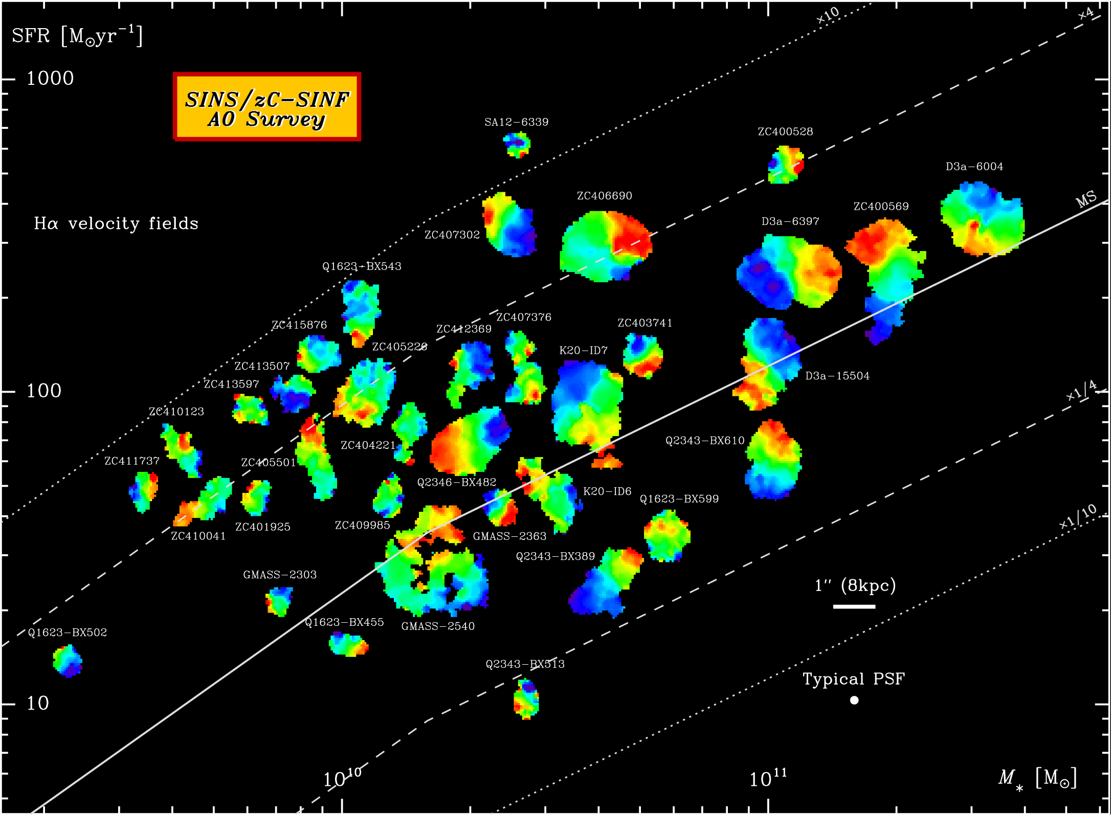