


Abstract
In the first orbit of the Parker Solar Probe (PSP), in situ thermal plasma and magnetic field measurements were collected as close as 35 RSun from the Sun, an environment that had not been previously explored. During the first orbit of PSP, the spacecraft flew through a streamer blowout coronal mass ejection (SBO-CME) on 2018 November 11 at 23:50 UT as it exited the science encounter. The SBO-CME on November 11 was directed away from the Earth and was not visible by L1 or Earth-based telescopes due to this geometric configuration. However, PSP and the STEREO-A spacecraft were able to make observations of this slow (v ≈ 380 km s−1) SBO-CME. Using the PSP data, STEREO-A images, and Wang–Sheeley–Arge model, the source region of the CME is found to be a helmet streamer formed between the northern polar coronal hole and a mid-latitude coronal hole. Using the YGUAZU-A model, the propagation of the CME is traced from the source at the Sun to PSP. This model predicts the travel time of the flux rope to the PSP spacecraft as 30 hr, which is within 0.33 hr of the actual measured arrival time. The in situ Solar Wind Electrons Alphas and Protons data were examined to determine that no shock was associated with this SBO-CME. Modeling of the SBO-CME shows that no shock was present at PSP; however, at other positions along the SBO-CME front, a shock could have formed. The geometry of the event requires in situ and remote sensing observations to characterize the SBO-CME and further understand its role in space weather.
Export citation and abstract BibTeX RIS

Original content from this work may be used under the terms of the Creative Commons Attribution 4.0 licence. Any further distribution of this work must maintain attribution to the author(s) and the title of the work, journal citation and DOI.
1. Introduction
Coronal mass ejections (CMEs) originating at the Sun propagate in the heliosphere and drive space weather at the Earth. The initiation and propagation of CMEs throughout the inner heliosphere need to be understood in order to better predict their geoeffectiveness. The Helios spacecraft made in situ measurements of a CME and its associated shock at 0.54 au (116 RSun; Burlaga et al. 1982). The CMEs were also measured by Helios over a range of distances such as 0.4 (Bothmer & Schwenn 1998) and 0.33 (Al-Haddad et al. 2019) au. The signatures were similar to those seen at 1 au, an increase in magnetic field strength, low density, and low plasma β. The Parker Solar Probe (PSP) enables the in situ measurements of the thermal plasma, magnetic fields, and energetic particles associated with CMEs at various stages of radial evolution closer than ever previously obtained and earlier in the evolution of the CME. The evolution of a CME from its initiation at the Sun through the heliosphere to Earth is a major focus of space weather research. Understanding the thermal plasma, particle acceleration, and magnetic structure of the CME is key to predicting its impact on space weather at the Earth or throughout the heliosphere.
The origin of CMEs is the instabilities connected to changes in the magnetic field of the corona (Gosling 1993). The observational structure and evolution of CMEs in coronagraph images may offer clues to the variety of phenomena with which they are associated at the Sun and thus provide insight into the initiation process(es) (Moore & Labonte 1980; Amari et al. 2003; Gopalswamy et al. 2006; Green et al. 2018; Georgoulis et al. 2019).
Ma et al. (2010) statistically analyzed the source locations of CMEs during solar minima and found that one-third of the CMEs in their study were "stealth" CMEs. These stealth CMEs are well-defined slow CMEs observed in coronagraph data with no identifiable surface or low coronal signatures (LCSs; Robbrecht et al. 2009; Ma et al. 2010; Wang et al. 2011; D'Huys et al. 2014; Kilpua et al. 2014; Lynch et al. 2016). Howard & Harrison (2013) stated that limitations in instrumentation and observation may lead to the identification of stealth CMEs. Indeed, Alzate & Morgan (2017) applied advanced image processing techniques to 40 previously identified stealth CMEs and found LCSs for each of the 40 events that would otherwise be hidden and thus allow for more accurate classification of these types of events. It stands to reason then that with proper image data processing, observable LCSs may exist for these slow-moving CMEs below the field of view (FOV) of coronagraph images. Regardless of nomenclature, these types of events exhibit characteristics in coronagraph data that parallel those of better-known CMEs. In their study of stealth CMEs, Ma et al. (2010) found that approximately half of them are of the blowout type CMEs. Vourlidas & Webb (2018) presented a comprehensive analysis of this particular class of CMEs known as "streamer blowouts" (SBOs; Sheeley et al. 1982). These events are characterized by a gradual swelling of the overlying streamer. The evacuation can take hours to days, and coronagraph data reveal signatures of a slow and well-structured flux rope. The SBO-CMEs are slow (vavg ∼ 390 km s−1) based on coronagraphic observations. They do not correlate with sunspot numbers, suggesting that they are not associated with active regions but originate from polarity inversion lines outside of active regions such as those associated with polar crown filaments. The SBO-CMEs are known to follow the tilt of the heliospheric current sheet (HCS; Vourlidas & Webb 2018).
Remote sensing observations can be combined with in situ particle and field measurements to study the dynamical evolution and propagation of CMEs. With STEREO, CMEs can be tracked from their initiation and subsequent propagation into the interplanetary medium up to 1 au, in which we can then measure in situ CME characteristics (Harrison et al. 2012; Lugaz et al. 2012; Nieves-Chinchilla et al. 2012, 2013; Temmer et al. 2012, 2017), which has improved our knowledge of CMEs and their evolution through space. Because of PSP, we are now able to measure the CME parameters at distances below 0.3 au, giving an unprecedented opportunity to have new insights and study the propagation and characteristics of CMEs in the early stages of their evolution.
Analytical and numerical models have been developed to investigate the CME propagation through the interplanetary medium, which is a fundamental issue in space weather forecasting. Analytically, most of the models describe a CME as an amount of mass and magnetic field expelled into space with a different speed from the solar wind. In the interplanetary medium, the gravity and Lorentz forces are assumed to be negligible, meaning that the CME kinematics depend on the CME and solar wind conditions (speed and density) and the way they interchange momentum during their interaction (Vršnak 2001; Cantó et al. 2005; Borgazzi et al. 2009; Vršnak et al. 2013, 2014).
Any of these models can predict the travel time, speed, and density, but they cannot predict the in situ parameter time profiles that can be observed at any heliospheric distance. This issue is addressed by the numerical models (Chen 1996; González-Esparza et al. 2003; Cargill 2004; Xiong et al. 2007; Shen et al. 2011, 2013; Lugaz et al. 2013). The physical basis for most simulations includes the gravitational, Lorentz, and/or aerodynamic drag forces. Various models are reviewed by Zhao & Dryer (2014) and Lugaz et al. (2017).
The focus of this paper is on utilizing the remote sensing and in situ data, as well as models, to understand the source, propagation, and lack of shock associated with the 2018 November 11 CME. Other papers in this issue address the magnetic structure (Nieves-Chinchilla et al. 2020) and energetic particles (Giacalone et al. 2020) associated with this CME. In Section 2, the remote sensing and in situ observations of the SBO-CME are reviewed. Section 3 details the modeling of the SBO-CME source on the Sun using the Wang–Sheeley–Arge (WSA) model and the propagation of the SBO-CME using a hydrodynamic model to simulate the CME to PSP and beyond. Included is a discussion of a flux rope propagation model and the lack of shock seen at 54.7 RSun. Section 4 ends the paper with a discussion of conclusions and future work.
2. Observations
STEREO launched in 2006 with two spacecraft: one leading (STEREO Ahead (STA)) and one lagging (STEREO Behind (STB)) the Earth's orbit at 1 au. On board STA, the imaging instrument package SECCHI includes two visible light coronagraphs, COR1 and COR2, as well as an extreme ultraviolet imager, EUVI. COR1 has an FOV from 1.5 to 4 RSun, while COR2 has an FOV that extends out to 15 RSun.
On 2018 November 10 at approximately 02:00 UT, STA COR1 (Howard et al. 2008) detected liftoff of a small CME. This event could not be observed from the Earth due to the geometric alignment between the Sun, Earth, and PSP. The CME was later measured in situ at PSP.
Figure 1 depicts a map with the locations of multiple solar-heliospheric spacecraft during the 2018 November 11–12 time period and helps to connect PSP and STA observations of this event with the estimated solar source region. From Earth's (green) location, PSP (orange) was located behind the Sun, almost perfectly aligned with the Sun–Earth axis, i.e., 178° HEEQ longitude, −1° HEEQ latitude, and 0.25 au (54 Rs). The location of PSP changes to 179° HEEQ longitude, −1° HEEQ latitude, and 0.26 au (56 Rs) over the observation period. In Figure 6, this is indicated with two vertical dashed lines. Figure 1 shows that STA (red) was located on the east side of the Sun at −103° HEEQ longitude, 6° HEEQ latitude, and 0.96 au. This configuration allowed remote observations by STA/COR2 of the transit of a slow SBO-CME on the plane of the sky (POS; marked with a red line in Figure 1) during the period between 2018 November 10 ≈10:00 UT and 2018 November 11 ≈06:00 UT. During this period, PSP was located at HEEQ longitude (165°, 173°), latitude (−2°,−2°), and heliocentric distance range of (0.22, 0.24 au). This position is marked with a brown curve in Figure 1.
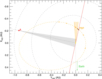
Figure 1. Map of the solar-heliospheric spacecraft: PSP (orange), STA (red), and Earth direction (green). The dashed orange oval indicates the orbit of PSP, and the solid orange curve is overplotted to indicate PSP's location during the time this event was observed in situ by PSP. The solid brown curve denotes the location of PSP for the period when the event was observed by STA/COR2. The COR2 FOV is delimited by the gray triangle. The orange triangle indicates the radial projection of the event mapped to the solar source region, as derived by the WSA model.
Download figure:
Standard image High-resolution imageThe orange triangle originating at the Sun and extending past the PSP orbit corresponds to the apparent opening angle of the SBO-CME in STA/COR2 observations (see Figure 2), from which we then assume a radial propagation of the SBO-CME out to PSP. This triangle funnels back to the estimated solar source region of this event, as derived by the WSA model (Arge & Pizzo 2000; Arge et al. 2003, 2004). The triangle's location indicated the source region with an angular width at the surface spans approximately 10° in longitude that represents the uncertainty in the solar source region. This width was estimated based on the model-derived longitudinal width of the helmet streamer and the change in longitude (due to solar rotation) of the STA east limb as the event propagates through the COR1/COR2 FOV. The analysis of the internal structure associated with the CME is discussed in detail in Nieves-Chinchilla et al. (2020), in this issue, and specific modeling parameters unique to the work on helmet streamers are described in Szabo et al. (2020), in this issue.
Figure 2. Remote sensing observations of the low corona by the SECCHI COR1 instrument on board the STA spacecraft. (a) The inner coronagraph, COR1, observes the corona from 1.4 to 4 Rs. The image shown was processed with a temporal filter with a transmission bandpass (N. Alzate et al. 2020, in preparation). The same method was applied to COR2 (panel (b)), which has an FOV out to 15 Rs. The FOV shown here spans from 3 to 15 Rs and thus overlaps with COR1 by about 1 Rs. An animation of this figure is available. The video begins on 2018 November 10 at 00:05:00 UT and ends the next day at 20:40:00 UT. The real-time duration is 8 s. On 2018 November 9 10:20 UT, the streamer belt brightens, signaling the beginning of the observation of the eruption, and the structure propagates through the FOV of the observation until 12:05 UT.
(An animation of this figure is available.)
Download figure:
Video Standard image High-resolution image2.1. Remote Sensing Observations of Propagation
STA observed a CME in COR2 on 2018 November 10. In COR1, the streamer belt brightened starting on 2018 November 9 at 10:20 UT and extended through the FOV for several frames. In Figure 2, panel (a) shows the bright front of this structure in COR1 as it nears the outer edge of the FOV at 12:05 UT. The online movie version for COR1 shows the expansion of the streamer and the evolution of the structure moving through it. Since the FOV of COR2 overlaps with that of COR1, we are able to track the structure into the FOV of COR2. Panel (b) of Figure 2 shows it entering COR2 at 12:08 UT. In Figure 3, we show a few EUVI frames from the 24 hr prior to the COR2 observation in panel (b). In the general region of interest, there is lots of activity in the form of low-density structures lifting from the Sun (indicated by the arrows). However, in EUVI, there is no obvious signature on the disk near the potential source region that we could identify as a potential source of flare activity associated with this event. The development of these structures across the EUVI FOV is best appreciated in the animation available online. Due to the nonradial nature of structures in this region of the corona, many of the structures observed at ±20°–30° from the equatorial region appear to follow a path that leads to the structures observed in COR1 and COR2, which is consistent with past observations during solar minimum configurations (Kilpua et al. 2009). Based on this and the fact that the streamer brightens in COR1 before the structure enters the FOV of COR2, we theorize that the CME formed at or below the inner FOV of COR1 (i.e., below 1.4 Rs). Proving or disproving this requires observations of the disk behind the Sun during this event, which do not exist.
Figure 3. Remote sensing observations of the low corona by the SECCHI EUVI instrument on board the STA spacecraft. The panels show the EUVI images of the solar disk and corona out to approximately 1.6 Rs for a few hours prior to two observations. These images were processed using the MGN technique (Morgan & Druckmüller 2014). The arrows point to a number of structures that escape from the Sun in the general region of interest. An animation of this figure is available. The video begins on 2018 November 6 at 00:14:00 UT and ends on 2018 November 11 at 22:09:02 UT. The real-time duration is 7 s. There are no obvious large-scale structures that erupt or solar flare activity observed in the EUVI animation. There are small low-density structures observed ±20°–30° from the equator of the Sun. These are consistent with other solar minimum observations.
(An animation of this figure is available.)
Download figure:
Video Standard image High-resolution imageA height–time map was generated for EUVI, COR1, and COR2 observations and is shown in Figure 4. The map was generated for a radial slice at an angle of 85° (counterclockwise from north). In it, a bright structure that lifted off in EUVI at the end of 2018 November 9 and reaches the edge of the FOV on 2018 November 10 is shown. This structure then appears to cross into the COR1 FOV and into the COR2 FOV at the end of the day. The structure appears to be fainter in COR1, at least near the inner edge, which may be a result of the difference in structure appearance between EUV and coronagraph observations. By the same token, structures have a different appearance in observations from inner coronagraphs when compared to those from outer coronagraphs, in this case, COR2. That being said, the method we used to process the data sets (N. Alzate et al. 2020, in preparation) suppressed high-frequency noise and low-frequency variations to allow us to track different structures as they cross all three FOVs.

Figure 4. Height–time map showing structures in the corona from 1 to 15 Rs generated from remote sensing observations (see Figure 3) with EUVI data at the bottom of the plot, COR1 in the middle, and COR2 in the top half of the plot. The FOVs shown extend out to 1.6 RSun for EUVI, from 1.6 to 2.8 RSun for COR1, and from 2.8 to 15 RSun for COR2. The black vertical rectangle in COR2 indicates a gap in the observations.
Download figure:
Standard image High-resolution imageTracking the front of the CME in the STEREO images enables the determination of the speed and duration of the CME, which are important characteristics to study the CME dynamics. We used the method described by Lara et al. (2004) in which the coronal brightness is computed at several heliospheric distances and in 11 position angle (PA) directions separated by 0 5 centered around the central position angle (CPA) for each available image. With this, it is possible to obtain the brightness as a function of time and distance.
With a Gaussian fit to the brightness as function of time, we compute a duration of the CME of Δt = 2.5 hr, and, by following the maxima, we plot the height in terms of time at the brightness maximum and the outer edge of the CME (nose). These acceleration profiles are shown in Figure 5. The nose of the CME was found to be moving at  km s−1 and the brightest part of the CME at
  km s−1 at Rinj = 6 R⊙. These velocity measurements are consistent with the observed mean speeds of SBO-CMEs during solar minimum (Vourlidas & Webb 2018). The gradual swelling of streamers caused by steadily injected magnetic energy will lead to low ejection speeds of the CME itself.
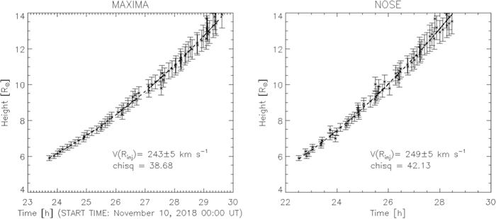
Figure 5. Height–time plot for the 2018 November 11 CME obtained with a Gaussian fit to the brightness as a function of time at different heliospheric distances using the method described by Lara et al. (2004). The left panel corresponds to the brightness maxima and the right panel to the nose of the CME. With the Gaussian fit, we compute  km s−1 at Rinj = 6 R⊙ and Δ t = 2.5 hr, values used to model the propagation of the CME at different heliospheric distances. In the case of the CME nose, we found that it is accelerating at 0.004 km s−2 by fitting a second-degree polynomial with a speed deviation of ±23 km s−1, while the CME brightest point accelerates at 0.006 km s−2 with a deviation of ±23 km s−1.
Download figure:
Standard image High-resolution image2.2. In Situ Thermal Plasma Measurements
In situ plasma data were collected by the Solar Wind Electrons Alphas and Protons (SWEAP) instrument suite (Kasper et al. 2016) on board PSP, which is currently orbiting the Sun with an initial perihelion of 35 RSun and an eventual perihelion of 9.86 RSun. The SWEAP instrument suite is made up of the Solar Probe Cup (SPC), SPAN-A (ions and electron measurements), and SPAN-B (electron measurements). The SPC (Case et al. 2020) is a Faraday cup that measures the temperature, density, and proton velocity at 0.825 s during encounter and every 28 s outside of encounter. The data plotted here are at a 28 s cadence. The SPAN electrostatic analyzers (Whittlesey et al. 2020) provided electron measurements used to create pitch angle distributions (PADs). The magnetic field data were collected by the FIELDS instrument suite (Bale et al. 2016). It provides the magnetic field vector components and magnetic magnitude. We plot 1 minute averaged magnitude data generated by the FIELDS team. This is an official data product and can be found on CDAWeb. It uses triangular averaging. The native cadence of the magnetic field data varies from 2.3 to 293 samples s–1 and can also be found on CDAWeb. For derived parameters such as plasma beta, we interpolated the FIELDS data to the SPC data. For large-scale structures such as this CME, the 1 minute data are more appropriate, as the full-resolution data would have multiple peaks and valleys associated with wave activity at short timescales that are not representative of longer intervals and general plasma characteristics discussed in this manuscript.
Figure 6 plots the in situ data from 2018 November 11–12. The CME is measured initially by PSP FIELDS and SWEAP at 23:50:45 UT on 2018 November 11 at a distance of 54.7 RSun or 0.25 au. This onset is marked in the plot by the leftmost black vertical dashed lines. The Radial, Tangential, Normal (RTN) coordinate system components of the proton speed data are plotted in panels (e) and (f). The average speed of the CME is v = 390 km s−1. The proton density is plotted in panel (g). The average density of the CME was ρ= 177 cm−3. The proton temperature is plotted in panel (h). The average temperature of the protons in the CME was found to be 7.3 × 10⁴ K. The plasma beta calculated using the data is plotted in panel (i). The β during the CME is always much less than 1. There is no clear shock structure associated with the CME. The start time of the CME was found by examining the increase in magnetic field that coincided with a rotation in field direction. The plasma data were also used as a marker of the start time with a lower temperature and the presence of bidirectional electrons.
The electron PADs are in panels (j) and (k) of Figure 6. The upper PAD panel has the raw flux represented, and the lower panel normalizes the flux at a particular angle to the mean flux over all pitch angles. Bidirectional electrons are known to be signatures of a CME and closed magnetic field configuration that either ends in a loop or is tied back to the Sun (Gosling et al. 1987). Bidirectional electrons are present when there are electrons at 0° as well as 180°, indicating that electrons were traveling both away from and toward the Sun. During the passage of the flux rope, there are bidirectional electrons present (for a more in-depth discussion of the flux rope structure, see Nieves-Chinchilla 2020, in this issue).
3. Discussion
3.1. CME Source Modeling
The combination of the in situ and remote sensing data gives information on the timing and characteristics of the CME. Utilizing this information, we can project the CME back to its source and learn about its coronal origin. In this work, the WSA model (Arge & Pizzo 2000; Arge et al. 2003, 2004) is used to derive the coronal field using a coupled set of potential field–type models. The first is a traditional magnetostatic potential field source surface (PFSS) model, which determines the coronal field out to the source surface height. The PFSS solution serves as input into the Schatten current sheet model to provide a more realistic magnetic field topology of the upper corona (e.g., from 2.5 to 21.5 RSun). An empirical velocity relationship (Arge et al. 2003, 2004) is then used to derive the solar wind speed at the outer coronal boundary. The model then propagates solar wind parcels outward from the end points of each magnetic field line, determining their time of arrival at PSP and thus providing the magnetic connectivity between 1 RSun and PSP magnetic field observations. The WSA model uses a simple 1D modified kinematic model, which accounts for stream interactions by preventing fast streams from bypassing slow ones (Arge et al. 2004).
Synchronic photospheric field maps used as input to the WSA model were generated using the Air Force Data Assimilative Photospheric Flux Transport (ADAPT) model (Arge et al. 2010, 2011, 2013) driven by Global Oscillations Network Group (GONG) magnetograms. ADAPT utilizes flux transport modeling (Worden & Harvey 2000) to account for solar time-dependent phenomena (e.g., differential rotation, meridional and supergranulation flows) when observational data are not available, making it particularly useful for studying this far-side event. Since ADAPT is an ensemble model, it provides 12 possible states (i.e., realizations) of the solar surface magnetic field, ideally representing the best estimate of the range of possible global photospheric flux distribution solutions at any given moment in time. When coupled with ADAPT, WSA derives an ensemble of 12 realizations representing the global state of the coronal field and spacecraft connectivity to 1 RSun for a given moment in time, providing an estimate of the uncertainty in the ADAPT–WSA solution. The best realization is then determined by comparing the model-derived and observed initial mass function (see Figure 3 of Szabo et al. 2020) and solar wind speed. While a magnetostatic potential field–based solution cannot capture time-dependent solar phenomena such as CMEs, ADAPT–WSA is used in this work to derive the coronal field pre-eruption and, in combination with in situ and remote sensing observations, deduce the solar source region of the SBO-CME. For a complete description of ADAPT–WSA and the parameters specific to the following model output, see Szabo et al. (2020).
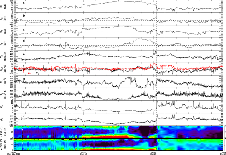
Figure 6. In situ measurements of the SBO-CME as it passes PSP at 57.4 RSun. Panel (a) plots the magnetic field strength as measured by the FIELDS instrument suite. Panels (b)–(d) plot the components of the magnetic field. Panel (e) plots the radial proton velocity, and panel (f) has the normal and tangential components of the proton velocity as measured by the SWEAP SPC. Panel (g) is the proton density. Panel (h) is the proton temperature. Panel (i) is the proton plasma beta. Panel (j) is the electron PAD, and panel (k) is the normalized electron PAD. The black vertical dashed lines indicate the arrival and departure times of the CME.
Download figure:
Standard image High-resolution imageFigure 7 shows the global corona and PSP connectivity to 1 RSun during corotation with the Sun, timestamped to best represent the coronal field as the underlying closed field of the SBO-CME source region begins to expand upward through the FOV of STA/COR1. Prior to this eruption, PSP corotates with a mid-latitude coronal hole of negative polarity shown in Figure 7 at approximately 335–340 Carrington longitude (CL) during Carrington rotation (CR) 2210. This coronal hole is comparable in size to STA/EUVI observations on 2018 November 14–18 when it rotates onto disk center after the eruption. According to ADAPT–WSA simulations, this coronal hole begins to close down and shrink after 2018 November 8 (see the coronal hole at perihelion in Figure 2 of Szabo et al. 2020) to its state in Figure 7. The PSP comes out of solar corotation, crosses the HCS, and magnetically connects to another mid-latitude coronal hole of positive polarity, shown in Figure 7 between 270 and 300 CL (CR 2210). The model-derived HCS crossing is ∼1 day earlier when compared to observations (Figure 3 of Szabo et al. 2020), likely due to the CME observed at PSP that is not captured by the model solution as discussed previously. The location where PSP traverses this helmet streamer (i.e., crosses the HCS) is highlighted with a blue oval in Figure 7.
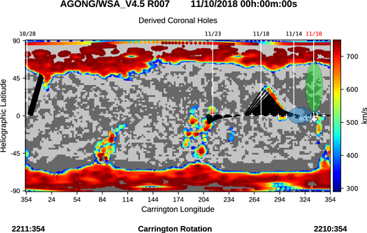
Figure 7. ADAPT–WSA derived coronal holes at 1 R⊙ with model-derived solar wind speed in color scale and PSP connectivity to the solar surface during the first solar encounter of PSP. The last GONG observations assimilated into the ADAPT input map were from 2018 November 11 00:00:00 UTC at approximately 174° CL (CR 2210). The field polarity at the photosphere is indicated by the light/dark (positive/negative) gray contours, where the boundaries of these contours reveal polarity inversion lines. White tick marks represent PSP's location mapped back to 5 R⊙ with dates given above in black. The date that the SBO-CME is first visible in STA/COR1 (2018 November 10) is labeled in red, showing the location of PSP at this time. Black lines show connectivity between the spacecraft and solar wind source region at 1 R⊙.
Download figure:
Standard image High-resolution imageBased on the location of PSP near the time the event is visible in COR1 (i.e., approximately −1° HEEQ latitude, 335° CL in Figure 7) and the observations of the event in COR1 (Figure 2(a)), there are only two plausible source regions of this eruption. One is the mid-latitude helmet streamer (HS) that PSP is connected to prior to the eruption (Figure 7, region in blue oval), and the other is the HS formed between the northern polar coronal hole and the negative mid-latitude coronal hole that PSP was connected to during corotation (Figure 7, region in green oval). To deduce the SBO source region, we first determined when this event becomes visible in STA/COR1. The first evidence of brightening and field expansion in COR1 is at approximately 02:00:00 UTC on 2018 November 10. We then aligned the WSA 3D coronal field solution with the STA COR1/COR2 FOV for this time period, shown in Figure 8, to see if either helmet streamer aligned with STA observations of this event on the east limb.
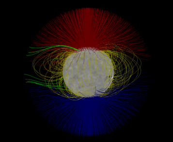
Figure 8. The 3D ADAPT–WSA derived coronal field for 2018 November 10 00:00:00 UTC, with the central meridian at 70° CL during CR 2210, aligned with STA as the field line expansion of this event becomes visible on the east limb in COR1 observations. Displayed are every 11th field line out to the PFSS solution of the model. Yellow field lines reflect the closed field, while red (blue) lines represent the outward/positive (inward/negative) open field. The field lines forming the helmet streamer cusp of the SBO-CME source region are highlighted in green, corresponding to the region in the green oval in Figure 7.
Download figure:
Standard image High-resolution imageFigure 8 shows a large helmet streamer on the east limb highlighted in green that corresponds to the region in the green oval in Figure 7. Assuming nearly radial propagation, the structure moving through the COR1 and COR2 FOV (Figure 2(a) and (b)) traces back to this model-derived HS cavity. This structure spans approximately 800–900 Mm at its 1 RSun base between the two coronal hole boundaries. The photospheric field beneath the helmet streamer cavity and in the surrounding region is rooted in the quiet Sun with an average photospheric field strength of  G according to ADAPT–GONG photospheric field observations. The identified source region is consistent with the description of SBO-CMEs in Vourlidas & Webb (2018), where these eruptions occur without the presence of an active region and result from the slow buildup of shear over time along the polarity inversion line, likely due to differential rotation.
3.2. Predicting the Arrival of the Slow CME at PSP
Having identified the coronal origin of the SBO-CME, we can now model the propagation from that source out to PSP and beyond. We examine the overall propagation through a simple solar minimum environment, as well as looking at the propagation of a flux rope model that allows for insight into the possible formation of energetic particles. We studied its evolution using a numerical simulation that followed the flux rope structure from its launch through its arrival at PSP (RPSP = 0.2543 au) in order to compare the simulated parameter time profiles with PSP in situ data.
The numerical simulation was done using the 2D hydrodynamic, adiabatic, and adaptive grid code YGUAZÚ-A, developed by Raga et al. (2000) and used previously to simulate the propagation of CMEs in the solar wind by Niembro et al. (2019). The code integrates the 2D Cartesian coordinate Euler equations for a full ionized plasma with a mean molecular weight μ = 0.62, in which the gas is assumed to be composed in mass fractions of the Sun by 0.7 H, 0.28 He, and 0.02 the rest of the elements.
In this model, the computational domain is filled by an isotropic flow with a mass-loss rate  , an initial speed
  , an initial temperature of 105 K, and with
  (with
(with  ) as the specific heat at constant volume. Then, the SBO-CME is imposed as a sudden change of the flow (to
  and
and  ) at the injection radius
  R⊙ during Δt and within a solid angle that corresponds to ϕ. Afterward, the solar wind resumes to V0 and
  .
.
This model was used because we have a solar minimum simplified configuration of the inner heliosphere. The CME moves radially, which means that the effects of curvature and the magnetic field are neglected. To study the propagation, hydrodynamic codes give reliable insights into the dynamics of CMEs in the solar wind. ENLIL models were compared to this model in Niembro et al. (2019), and the results with ENLIL are similar due to the radial propagation of the CMEs. The results are consistent between both models, as the magnetic field contribution can be neglected and its contribution is within the uncertainties.
The initial SBO-CME speed  km s−1, mass MCME = 2.1 × 10¹⁵ g, duration Δt = 2.5 hr, and angular width ϕ ∼ 20° were computed following Lara et al. (2004) and from the height–time plot shown in Figure 5 assuming the injection time on 2018 November 10 23:54 UT at Rinj = 6 R⊙, in which COR1 STA was tracking the SBO-CME. For the CME mass, we estimate the mass at each pixel as m = (Bobs/Be) × 1.97 × 10⁻²⁴ g, with Bobs the observed brightness and Be the brightness of a single electron (Colaninno & Vourlidas 2009; Vourlidas et al. 2010). Here Be was computed using the model described by Billings (1966). We calculate the total mass by summing the values in the region, limited as per the model of Thernisien et al. (2009), in the image that contains the CME. With this value, we calculate the CME mass-loss rate to be
  × 10−14 M⊙ yr−1. The mass-loss rate is a minimum value due to the assumption that the mass is in the POS and not in a 3D structure. Due to the narrow nature of the CME, the error in mass estimate could be as high as 50%, as reported by Colaninno & Vourlidas (2009).
For this particular event, we considered that the ambient solar wind conditions are slightly different before and after the SBO-CME. The initial conditions of the ambient solar wind prior the SBO-CME ( and
and  ) expected at Rinj were derived using the estimated PSP in situ measurements of VPSP = 380 km s−1 and nPSP = 200 cm−3 computed during the interval of time from 2018 November 11 23:45 UT to 2019 November 11 23:50 UT. By solving the equations described in Cantó et al. (2005), we estimate that at Rinj, the speed of injection is
  372 km s−1. Then, we compute a mass-loss rate of
  4π
4π  NPSP VPSP = 2.4 × 10⁻¹⁴ M⊙ yr1. For the ambient solar wind behind the CME, we used the average PSP measurements of VPSP = 400 km s−1 and nPSP = 200 cm−3 computed during the interval of time from 2018 November 12 06:37 UT to 2018 November 12 07:35 UT and found that this flow was injected at Rinj with
  and
and  –392 km s−1.
In Figure 9, we show the results of the model (green solid line with colored star symbols) overplotted on the SWEAP/SPC in situ thermal plasma data (black solid lines). YGUAZÚ-A allowed us to tag the different plasma components, which we have marked with colored symbols: the solar wind in front of the SBO-CME in blue, the SBO-CME in red, and the solar wind behind the SBO-CME in green. The colored symbols allow us to hydrodynamically identify these different plasma components and determine the arrival time of the flux rope.

Figure 9. SWEAP/SPC in situ measurements. From top to bottom: magnetic field magnitude B, speed magnitude V, proton density NP, and kinetic energy WP. The green solid line shows the predicted speed and density time profiles, and the colored symbols tag the solar wind in front of the SBO-CME in blue, the SBO-CME in red, and the solar wind behind the SBO-CME in green. Black dotted lines mark the initial time of the CME, the arrival of the flux rope, and the end of the CME. A red dashed line shows the arrival time predicted by the model. This time is comparable with the end of the CME observed in the in situ measurements; as we are modeling a slow CME, the HD model tracks the transition between the CME and the solar wind behind it.
Download figure:
Standard image High-resolution imageWith black dotted lines, we show the initial and final times of the SBO-CME observed at PSP (from 2018 November 11 23:50 UT to 2018 November 12 06:36:19 UT) and the arrival of the flux rope (2018 November 12 04:15 UT). With the numerical model, we predict the arrival of the end of the flux rope in the slow SBO-CME. The model requires a density transition from the CME (red symbols in Figure 9) and the ambient solar wind (green symbols) to indicate that the perturbation (SBO-CME) is present within the ambient solar wind. In this case, due to the fact that it is a slow CME, the flux rope interacts with the solar wind behind it. Using the model results, we find that the flux rope arrives 30 hr after launch (shown in the figure with a dashed red line) with a speed of 383 km s−1 with a difference of 0.33 hr and 2 km s−1 from the SWEAP/SPC measurements.
It is important to notice that due to the fact that we are not modeling the CME magnetic field structure, our density prediction during the CME is not comparable to the observations. However, before and after the CME, our results accurately predict the solar wind density value.
With the simulation, we also predict that at 14 R⊙, the CME reaches a speed of 374 km s−1, which can be compared with the observations plotted in Figure 5. According to the observations, at 14 R⊙, the CME reaches a speed of 347.61 ± 37.14 km s−1 (∼375.58 ± 23 km s−1 with the second-degree polynomial), which is, within the uncertainties, comparable with the one we obtain with the simulation at this particular distance.
3.3. SBO-CME Flux Rope Propagation Model
The CME discussed here is a very weak event, and no shock-sheath system can be identified in the images during the eruption of the CME or in the in situ plasma data at PSP. Energetic particles were seen at PSP around the arrival time of the SBO-CME (details in Giacalone et al. 2020, this issue). Here we have modeled this CME from the source to PSP using a forward modeling technique that is detailed in Rouillard et al. (2020) to explore the possibility of the solar energetic particle (SEP) being associated with this SBO-CME. The flux rope structure assumed in the present work is a bent toroid with an exponential increase of its cross-sectional area from footpoint to apex. Narrow CMEs have been shown in past STEREO studies of previous events to correspond to a flux rope in the shape of a bent toroid such that its major axis is located in a plane containing the line of sight of the observing spacecraft (e.g., Thernisien et al. 2009). Additionally, the flux rope model has an internal magnetic field structure described analytically inside the envelope of the CME.
The forward modeling technique proceeds via manual iterations until a good fit of the flux rope is obtained to the available observations. The fitting procedure is essentially very similar to the one proposed by Thernisien et al. (2009) and Wood et al. (2010). Unfortunately for this event, we do not have imaging from multiple vantage points because the event was very weak and erupted on the far side of the Sun; therefore, it could not be seen by near Earth–orbiting spacecraft. Hence, compared to the COR-2A images, the model assumes that the CME erupts close to the POS. The imaging observations were not sufficient to confirm the longitudinal extent of the legs of the flux rope, and this is an uncertainty of the present fitting. Figure 10 shows a set of coronagraphic observations from COR-2A in which we overplot the 3D modeled flux rope.

Figure 10. Running-difference COR-2A images of the CME without (left panel) and with (right panel) the shape of the 3D modeled flux rope used for the fitting.
Download figure:
Standard image High-resolution imageThe flux rope model is performed to the outer extent of COR-2A, where we find that the CME acceleration phase has nearly ended and the CME speed is almost constant (380 km s−1). The results of the CME kinematics are presented in Figure 2 of the extended data in McComas et al. (2019). By propagating the flux rope at a constant speed of 380 km s−1 from the time the CME exits the COR-2A FOV to PSP, we "predicted" an impact of the CME at PSP on November 12. The predicted arrival time and the magnetoplasma properties of the CME from this flux rope model are in very good agreement with those measured in situ by the FIELDS and SWEAP instruments, as seen in Figure 6 and the model speed of v ≈ 383 km s−1. The CME modeling presented here provides a good description of the CME evolution from the upper corona to PSP.
To investigate the possible formation of a shock associated with this SBO-CME, the above flux rope model is utilized to model the behavior from the COR2 FOV to PSP. To derive the 3D properties of the modeled coronal pressure/shock wave that could have formed around the expanding flux rope, we use methods presented in previous papers (e.g., Rouillard et al. 2016; Plotnikov et al. 2017; Kouloumvakos et al. 2019) but adapted in this study to use a flux rope rather than an ellipsoidal structure typically used for more energetic events. We start with the sequence of the regularly time-spaced flux ropes and consider a set of grid points distributed over the surface. From the sequence of the time-spaced flux rope grid points, we calculate the 3D distribution of velocity vectors at each point on the surface of the flux rope. The 3D speed is plotted in Figure 11 (panel (a)).
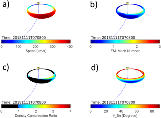
Figure 11. Results of modeling the flux rope during its propagation from the Sun to PSP. The derived parameters are plotted on the surface of the flux rope; they include the 3D plasma speed at each point on the surface of the flux rope (panel (a)), MFM number (panel (b)), density compression ratio (panel (c)), and θBn (panel (d)). The black regions in panel (c) correspond to regions where no shock could form. The blue line is the nominal Parker spiral extending from PSP to the Sun.
Download figure:
Standard image High-resolution image
As already stated, for this weak CME event, we do not observe the clear sheath and shock structure typically observed in more energetic CMEs (see, for example, Kwon & Vourlidas 2017; Kouloumvakos et al. 2019). So we assume that if a weak shock formed, it should be located near the surface of the flux rope due to the CME interaction with the background solar wind. That could result in a very weak and narrow sheath region. Then we use a model for the background solar wind to compute the wave properties and determine if there are regions where a shock forms. We exploited the plasma and magnetic field properties from the magnetohydrodynamic coronal and solar wind model produced by Predictive Sciences Inc. (courtesy of Jon Linker and Pete Riley). The Magnetohydrodynamic Around a Sphere Thermodynamic model is an MHD model developed by Predictive Sciences Inc. that makes use of the photospheric magnetograms from SDO/HMI as the inner boundary condition of the magnetic field and includes detailed thermodynamics with realistic energy equations accounting for thermal conduction parallel to the magnetic field, radiative losses, and parameterized coronal heating (Lionello et al. 2009; Riley et al. 2011). Details of the model and synoptic figures of the cubes used in this study can be found on the PSI site.17 We have also uniformly scaled the values of density, magnetic field, and temperature to match as well as possible the solar wind properties measured by the PSP SWEAP and FIELDS instruments just before the CME impacted the spacecraft.
Combining the flux rope fitting technique with the background solar wind model with the methods presented by Kouloumvakos et al. (2019), we can compute at each point on the surface of the flux rope the fast magnetosonic Mach number (MFM; panel (a)), the density compression ratio (panel (c)) by solving the Rankine–Hugoniot relations, and the magnetic field obliquity with respect to the flux rope shock normal (θBn; panel (d)). We also traced in blue in Figure 11 the trajectory of the nominal Parker spiral. Figure 11 shows that throughout its transit to PSP, the CME did not produce a shock in the region magnetically connected with the probe; the region where the Parker spiral (blue line) intersects with the flux rope remains back in panel (c), and the Mach number is always below 1. However, the calculations show that weak shock solutions with Mach numbers greater than 1 but below critical values do appear over a region at the western flank of the flux rope that are not connected with PSP. The subcritical shock in these regions is driven by the lateral expansion of the CME moving at less than 50 km s−1 in the orthoradial direction in a background solar wind flow that is moving predominantly in the radial direction. The ability of slow CMEs to compress the background solar wind and produce weak shocks in response to the expansion of the flux rope has been discussed and studied in past papers analyzing STEREO data (Rouillard et al. 2011; Lugaz et al. 2017).
4. Conclusions
We have presented PSP observations of an SBO-CME on 2018 November 11 starting at 23:50 UT. This was the closest to the Sun in situ measurement of a CME to date. The SBO-CME was also seen in remote sensing observations by STA. This event could not be seen from Earth due to the geometric configuration. This work has examined the source of the CME, its propagation to PSP, and the in situ measurements. The structure of the SBO-CME seen at PSP does not have a shock sheath normally associated with CMEs. This study has looked at the source of this CME that could not be seen at Earth, as well as modeled it through a solar minimum inner heliospheric environment. The coronal source of this SBO-CME was modeled using the WSA model to determine that the source region of the SBO-CME is the helmet streamer on the eastern limb as viewed by STA. This result, in combination with the slow rise of this event in COR1 observations (Figure 2) and slow solar wind speeds observed at PSP/FIELDS for this eruption (Figure 6), is consistent with Vourlidas & Webb (2018), who showed that SBO-CMEs likely originate from quiet Sun photospheric field, where shear builds up slowly over time along the polarity inversion line.
The kinetics of this young, still-evolving CME tells us about propagation through a solar minimum environment. Modeling using a hydrodyanmic model gives consistent predictions for the arrival time at PSP. Although 65% of CMEs at 1 au were found to have shocks associated with them (Jian et al. 2006), no shock was associated with the CME at PSP at 54.7 RSun. We do find evidence in the flux rope model that a highly quasi-perpendicular but weak and subcritical shock (Mach less than 2) could have formed over a narrow region at the west flank of the CME flux rope. The ability to accelerate particles at the shock front is key in understanding the origin of energetic particles that create space weather hazards. Understanding the interaction of the CMEs with the interplanetary space that they propagate through will help in understanding the sources of these hazards. In addition, this isolated event could be compared to other multiple events, such as those seen in 2019 April (Schwadron et al. 2020), which has implications for the creation of seed particles for SEPs and more geoeffective events.
The geometry of this event illustrates the need for multipoint observations and multiple data sets. One singular data set would not have enabled the tracing of an SBO-CME from its coronal source to PSP and beyond. It would have been undetected from the Earth. Understanding of the CME production rate of the Sun and the ability of CMEs to affect space weather throughout the heliosphere is aided by PSP observations at various radial distances. Future work will examine the other CME from encounter 1 on October 31 to further characterize the sources and inner heliosphere propagation of SBO-CMEs.
We acknowledge the NASA Parker Solar Probe mission and the SWEAP team led by J. Kasper for use of data. We gratefully acknowledge NASA contract NNN06AA01C. N.P., A.K., and A.P.R. acknowledge financial support from ANR project COROSHOCK ANR-17-CE31-0006-01 and ERC project SLOW_SOURCE - DLV-819189. We thank Jon Linker and Pete Riley of Predictive Sciences Inc. for providing the background solar wind model exploited in this study. S.D.B. acknowledges the support of the Leverhulme Trust Visiting Professor program We thank all of the people that have made the Parker Solar Probe the bold mission it is. This includes but is not limited to Peter Dagineau, David Caldwell, David Curtis, Tony Mercer, Michael Ludlam, Chris Scholtz, Andrew Peddie, Matt Reinard, Steve Jordan, Kathleen Entler, Brenda Bernard, Nick Pinkine, Kim Runkles, Luke Becker, Jim Kinnison, Nicola Fox, Andy Driesman, and Patrick Hill.
Facilities: STEREO. -