


Abstract
Understanding the properties of stellar populations and interstellar dust has important implications for galaxy evolution. In normal star-forming galaxies, stars and the interstellar medium dominate the radiation from ultraviolet (UV) to infrared (IR). In particular, interstellar dust absorbs and scatters UV and optical light, re-emitting the absorbed energy in the IR. This is a strongly nonlinear process that makes independent studies of the UV-optical and IR susceptible to large uncertainties and degeneracies. Over the years, UV to IR spectral energy distribution (SED) fitting utilizing varying approximations has revealed important results on the stellar and dust properties of galaxies. Yet the approximations limit the fidelity of the derived properties. There is sufficient computer power now available that it is now possible to remove these approximations and map out of landscape of galaxy SEDs using full dust radiative transfer. This improves upon previous work by directly connecting the UV, optical, and IR through dust grain physics. We present the DirtyGrid, a grid of radiative transfer models of SEDs of dusty stellar populations in galactic environments designed to span the full range of physical parameters of galaxies. Using the stellar and gas radiation input from the stellar population synthesis model PEGASE, our radiative transfer model DIRTY self-consistently computes the UV to far-IR/sub-mm SEDs for each set of parameters in our grid. DIRTY computes the dust absorption, scattering, and emission from the local radiation field and a dust grain model, thereby physically connecting the UV-optical to the IR. We describe the computational method and explain the choices of parameters in DirtyGrid. The computation took millions of CPU hours on supercomputers, and the SEDs produced are an invaluable tool for fitting multi-wavelength data sets. We provide the complete set of SEDs in an online table.
Export citation and abstract BibTeX RIS
1. Introduction
The ultraviolet (UV), optical, and infrared (IR) emission of a galaxy reflects the underlying populations and distributions of stars, gas, and dust, excluding any contributions from an active galactic nucleus. The detailed shape of a galaxy's integrated spectral energy distribution (SED) contains information about both the stellar populations (e.g., total stellar mass, stellar mass-to-light ratio, star formation history, and metallicity) and the interstellar medium (ISM; e.g., total dust mass, grain composition, and size distribution). These quantities probe the stars themselves and the fuel for star formation and thus are crucial to understanding galaxy formation and evolution. While integrated SEDs do not provide measurements for spectral indices or equivalent widths of absorption and emission features, when compared to high resolution spectra they are much easier to obtain, and hence enable studies on large-scale surveys of galaxies both locally and at a range of redshifts.
Modeling of the intrinsic stellar spectra starts from the initial mass function (IMF), which describes the distribution of newly formed stars and is generally based on power laws with adjustments at the very high and low mass limits (e.g., Salpeter 1955; Kroupa 2001). Combined with stellar evolutionary tracks and stellar spectra, Tinsley (1968) and many others created stellar population synthesis models to compute the detailed spectra of single stellar populations. Charlot & Bruzual (1991) developed an isochrone synthesis method that solved the problems in modeling fast evolutionary phases caused by sparsely sampled stellar evolutionary tracks. Padova isochrones (Bertelli et al. 1994) include a wide range of stellar ages and metallicities, and they cover most of the important evolutionary phases, including the thermally pulsing regime of the asymptotic giant branch.
The composition of interstellar dust grains has been inferred based on their extinction and emission. The three major dust components present in the diffuse ISM of the Milky Way (MW) include silicate, carbonaceous, and polycyclic aromatic hydrocarbons (PAH) grains. The major dust extinction features are the 2175 Å absorption feature, identified as due to small graphite grains (Stecher & Donn 1965) and the absorption features at 9.7 and 18 μm that are attributed to silicate grains (Willner 1976; McCarthy et al. 1980). The mid-infrared aromatic features found between 3 and 18 μm are associated with PAH grains (Leger & Puget 1984; Allamandola et al. 1985). The bulk of the dust emission is seen in the far-infrared and well modeled by large silicate and carbonaceous grains (Desert et al. 1990; Li & Draine 2001).
The presence of dust grains significantly alters the UV-optical spectra of galaxies by absorbing and scattering photons. The wavelength dependence of these effects along a single sightline toward a star is characterized by an extinction curve. The major features of the dust extinction curve are a general increase in extinction with decreasing wavelength, the far-UV rise, and the aforementioned 2175 Å bump (see Figure 4). Although the strength of these features varies along different sightlines, Cardelli et al. (1989) found that the average extinction curve in both diffuse and dense regions of the MW can be described by an extinction law that depends on only one parameter,  , where A(V) is the total V band extinction and
  is the selective extinction between the B and V bands. The standard method to determine extinction curves is the "pair method," which takes advantage of the fact that the intrinsic spectra of a reddened star (one that suffers from dust extinction) and an unreddened star of the same spectral type should be the same (Stecher 1965). However, extinction curves only apply to the simple geometry of a star observed through a screen of dust. Galaxies have more complex geometries where the effects of mixing the stars, gas, and dust must be taken into account. The inclusion of dust radiative transfer effects (e.g., different stars seeing different dust optical depths and scattered photons included in the measurement) changes the effects of dust from the geometry invariant extinction curve to those of an attenuation curve with a shape that is dependent not only on the properties of the dust grains, but also the relative distributions of stars, gas, and dust (Witt & Gordon 2000).
The energy absorbed by dust grains in the UV-optical is primarily emitted in the IR. In the simplest case, the far-IR dust emission spectrum resembles a modified blackbody with an emissivity β that may vary depending on composition and environment (e.g., Lis et al. 1998). Schlegel et al. (1998) found that the temperature of the far-IR dust emission in the MW is on the order of 20 K, which corresponds to a peak of emission around 150 μm. While the far-IR dust emission can be modeled as modified blackbody emission with a single temperature, the mid-IR emission is more complicated to calculate, as the dust emission in this wavelength range is dominated by stochastically heated dust grains (Leger & Puget 1984). Stochastic heating is also known as transient or non-equilibrium heating.
SED fitting is a widely used method to recover stellar, gas, and dust properties of star-forming regions and galaxies. Thanks to various space missions such as the Galaxy Evolution Explorer (GALEX; Martin et al. 2005) in the UV, the Spitzer Space Telescope (Spitzer; Werner et al. 2004) in the mid- to far-IR, and the Herschel Space Observatory (Herschel; Pilbratt et al. 2010) in the far-IR to sub-mm, we have high quality photometric data in the wavelength ranges that are crucial to SED fitting but not observable on Earth due to the opaque atmosphere. Combined with ground based optical and near-IR data such as those from the Sloan Digital Sky Survey (SDSS; Gunn et al. 2006) and Two Micron All Sky Survey (2MASS; Skrutskie et al. 2006), respectively, we have an abundance of well sampled UV to IR/sub-mm SEDs of star-forming galaxies.
The wealth of UV to far-IR SEDs of galaxies has been used in many studies to investigate the properties of galaxies. Calzetti et al. (2000) fit the far-IR SEDs of eight local starburst galaxies with two modified blackbody functions and found that cool dust contributes up to 60% of the total far-IR emission and is up to 150 times more massive than warm dust. By fitting the UV-optical SEDs of ∼50,000 optically selected local galaxies to a library of dust-attenuated population synthesis models, Salim et al. (2007) obtained dust-corrected SFRs of these galaxies and calibrated a simple prescription to obtain such SFRs with only GALEX far-UV and near-UV data. Erb et al. (2006) fit the observed 0.3–8 μm SEDs of 87 rest-frame UV-selected star-forming galaxies at  to Bruzual & Charlot (2003) population synthesis models and the Calzetti et al. (2000) extinction law, and found that metallicity monotonically increases with the derived stellar mass.
Dusty SED fitting in the literature generally falls into three categories: (1) UV-optical SED fitting (e.g., Salim et al. 2007, (2) infrared SED fitting (e.g., Draine et al. 2007), and (3) full UV to infrared SED fitting with the UV-optical and infrared connected in simple ways (e.g., Noll et al. 2009). Fitting UV and optical observations alone results in significant degeneracy between the age of the stellar population and the amount of dust present. Fitting the IR observations alone results in knowledge of the IR properties of dust grains, but very little about the underlying stellar populations or UV dust properties. Due to the nonlinear interaction between dust and the radiation field, a complete solution to the full UV to infrared SED requires 3D dust radiative transfer, which is computationally intensive. By requiring that the absorbed energy in the UV-optical equals the energy emitted in the infrared, one can connect the UV-optical to the infrared without radiative transfer. While to zeroth order correct, such a simple method does allow models that can violate dust physics in that the detailed IR dust emission SED is not dependent on the wavelength dependence of dust absorption and the dust grain properties, but only on the integrated dust absorption.
A more powerful but historically impractical way is to fit the full UV to infrared SED with the UV-optical and infrared connected by dust radiative transfer physics. Galaxies have complicated global and local 3D geometries of stars and dust, and these geometries strongly influence the dust radiative transfer solution (Witt et al. 1992; Witt & Gordon 1996, 2000). Such 3D dust radiative transfer has no analytic solution (Steinacker et al. 2013). With advances in computer performance and the availability of supercomputing clusters dedicated for science, a large scale computation to map out the SED landscape with radiative transfer has become possible. Variations in stellar and dust properties cause simultaneous changes in the UV-optical and infrared SED. Full radiative transfer solutions allow us to use the full information content of the SEDs to constrain the model of a galaxy. Information carried in each part of the SED is complementary with the other part, and by simultaneously solving for both, we can break degeneracies in stellar and dust parameters.
We present the DirtyGrid in this paper. DirtyGrid is a grid of UV to IR SEDs built from a combined dust radiative transfer and stellar population synthesis model. To capture to whole SED landscape, the grid spans a large range of eight parameters: stellar age, metallicity, stellar surface density, star formation type, amount of dust, global geometry, dust clumpiness, and grain type. A potential ninth parameter would be the IMF, which we have chosen to fix as Salpeter (1955). We describe the underlying models used to build DirtyGrid, explain the choice of parameters, and present the resultant SEDs. In the next paper in this series, we will use the DirtyGrid to study dust properties in nearby galaxies and test various star formation rate (SFR) indicators commonly used in the literature.
2. Defining the Inputs
The DirtyGrid is a set of model SEDs of stellar populations with dust and gas, distributed in a eight-dimensional parameter space. For computational purposes, the parameter space is discretized into a grid, and it is customary to call DirtyGrid a grid of models. At each grid point, the SED is either (1) constructed using the DIRTY radiative transfer model (Gordon et al. 2001; Misselt et al. 2001), or (2) interpolated from nearby grid points constructed using DIRTY, in order to conserve computations when the change in the SED is small. Figure 1 shows an example DirtyGrid SED. The grid of models is designed to span the possible range of stellar, dust, and geometric parameters of stellar populations in galactic environments. Under the assumption that the UV–IR SEDs of normal star-forming galaxies are dominated by one or a few types of characteristic star-forming regions unique to each galaxy, we can use combinations of models in the grid to fit whole galaxies. In this section, we describe the DIRTY radiative transfer model and the inputs that define the parameter space covered by the DirtyGrid models.
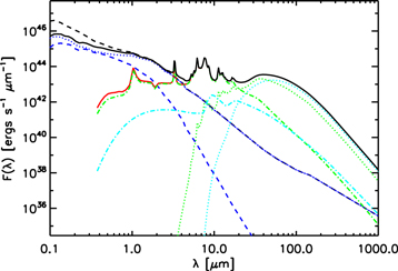
Figure 1. Example global SED for a young (10 Myr) stellar population, with a stellar mass of 1010 M☉, Milky Way type dust, a 10 kpc radius, a Shell geometry, and an optical depth of  . The dashed black line is the input stellar SED. The solid black, blue, and red lines are the total output SED, the radiative transfer component (extinguished plus scattered), and the total dust emission. The dotted and dashed components give the direct and scattered stellar component of the radiative transfer component. Among the dust emission components, the green and light blue lines represent carbonaceous and silicate grains; the dotted and dashed-dotted lines represent equilibrium and stochastic dust emission, respectively.
Download figure:
Standard image High-resolution image2.1. Radiative Transfer—DIRTY
Due to the ability of dust to absorb, scatter, and re-emit radiation, deriving the global SED of a stellar population mixed with interstellar dust is a radiative transfer problem. The three-dimensional (3D) radiative transfer problem can be represented by an integral-differential equation (Steinacker et al. 2013). However, in the general case, this equation has no analytic solution. We use DIRTY, a 3D Monte Carlo model to compute the radiative transfer of stellar, gas, and dust emission through a dusty medium. DIRTYv1 is described in detail in Gordon et al. (2001) and Misselt et al. (2001). The current version of the code (DIRTYv2) is based on the algorithms in DIRTYv1, but with the addition of a full dust grain model, a tighter integration of the dust radiative transfer and emission calculations, improved robustness of the input/output, and the enhancement of continuous photon absorption to accelerate the calculations. Here we provide a summary of DIRTY and detail the new features in the current version. Readers interested in the radiative transfer details should refer to the original DIRTY papers and Steinacker et al. (2013).
A single run of a DIRTY model requires three inputs: (1) the energy sources, (2) the physical properties of the absorptive medium (e.g., the dust grain physics), and (3) the relative distribution of both dust and stars: the model geometry. In the context of a DIRTY model, "geometry" refers to both the relative distribution of sources and dust throughout the model space (global geometry), as well as the clumpiness of the dust distribution (local geometry). By construction, in DIRTY all three ingredients may be arbitrarily specified. In general, the inputs are specified based on the physical problem at hand. While the local geometry can be of arbitrary complexity (e.g., independent dust densities at each point in the model space), it is convenient to specify the local distribution of dust ("clumpiness") by a two-phase medium characterized by the filling factor of high density regions embedded in a uniform medium and the density ratio between the high density regions and the uniform medium (Witt & Gordon 1996).
DIRTY has two main components: a radiative transfer routine and a dust emission routine. Given a distribution of emission sources within an absorptive medium, the purpose of the radiative transfer routine is to calculate the distribution of absorbed and escaped fluxes according to the physics of the interaction between photons and dust grains and the relative distribution between the sources and the dust. The same radiative transfer routine is used for both primary emission (from stars and gas) and secondary emission (from dust). The dust emission routine calculates the emission spectrum from the absorption spectrum according to the physics of dust heating and cooling. The fact that dust emission can be re-absorbed by dust during radiative transfer introduces a circular dependency between the dust absorption and emission spectra, so DIRTY takes an iterative approach to obtain a self-consistent solution. The iterative procedure is illustrated in Figure 2. This contrasts with the simpler way of modeling dust heating with a radiation field scaled from observations in the solar neighborhood (e.g., Draine et al. 2007).
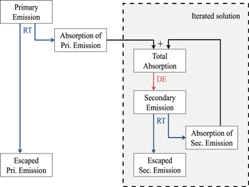
Figure 2. Iterative procedure used in DIRTY to achieve a self-consistent radiative transfer solution. Primary emission refers to emission from stars and gas; secondary emission refers to emission from dust. The radiative transfer and dust emission routine are denoted as RT and DE, respectively. The iterated solution procedure is repeated until convergence is achieved (e.g., the direct plus scattered light changes are below a specified threshold), after which we combine escaped primary and secondary emissions to obtain the final SED.
Download figure:
Standard image High-resolution imageThe DIRTY radiative transfer algorithm utilizes a weighted Monte Carlo approach with absorption-scattering split, forced first scattering, the peel-off technique, and continuous absorption, which are summarized below. We use a Cartesian local mean intensity storage grid to discretize the model geometry into regions of constant optical depth and radiation fields (see Section 2.4 for details). Steinacker et al. (2013) reviewed 3D dust radiative transfer techniques in general (not specific to DIRTY) and devoted a section to each of the performance enhancing techniques we list above. For the same level of accuracy achieved, these techniques allow us to reduce the amount of computation required, which is critical for a large scale project like the DirtyGrid. Alternatively, for the same computation time, one could use these techniques to enhance the accuracy of the results.
In the weighted Monte Carlo approach, instead of following individual photons as discrete particles, we assign weights to photon packets and keep track of the changes in the weights due to interaction events. We trace the trajectory of a photon packet and determine the distance traveled according a random number sampled from a probability distribution based on the optical depth in the path. At each interaction site, we split the weight of the photon packet into an absorbed portion and a scattered fraction according to the dust albedo (the absorption-scattering split). The direction of scattering is determined from a scattering phase function. Instead of depositing the entire absorbed portion at the interaction site, we distribute the energy along the path. This is known as continuous absorption and is new to DIRTYv2. In addition, we allow the photon packet to contribute to the escaped flux at each interaction site to improve the spatial sampling (the peel-off technique). In low optical depth models, a large number of photon packets may exit the model geometry without any interactions. To avoid "wasting" photon packets, we force the first scattering so that all of them contribute to the absorbed and scattered fluxes, and we correct for the bias in probability by adjusting the weights.
For a fixed number of interaction events, continuous absorption greatly improves the sampling of the radiation field while keeping the sampling of scattering the same. However, this calculation is relatively expensive. As a result, for a fixed amount of computation, this technique improves the determination of the local radiation field but worsens the sampling of scattering. In other words, it shifts the computational balance to focus more on populating the radiation field. For the parameter space covered by the DirtyGrid, this is beneficial because usually the scattered fluxes are better populated than the radiation field, and stochastic heating of dust grains is very sensitive to noise in the radiation field. Conversely, continuous absorption may not be suitable for models of extremely high optical depth or models that only calculate the equilibrium emission of dust grains.
We repeat the radiative transfer for a number of photon packets until the Monte Carlo uncertainty in the direct and scattered fluxes is below a desired limit (0.5%–1.0%, depending on the geometry), or until the maximum limit of 10 million photon packets per wavelength has been reached. We then repeat the process for all the wavelengths in a non-uniform wavelength grid with 174 points. This wavelength grid is composed of a uniform grid in log wavelength between 0.0912 and 1000 μm, with extra points placed to sample where there are features in the dust absorption, scattering, or emission (e.g., the mid-infrared for the PAH emission features and silicate absorption features). Including more points would not change the solution, as the relevant dust features are well sampled, while including fewer points would result in an inaccurate solution.
2.2. Stellar Populations
Since DirtyGrid is intended to provide a grid of integrated galactic SEDs over a large range of properties, the sources for the radiative transfer model are stellar population models. Stellar population models calculate the integrated SEDs of stellar populations optionally including the emission due to ionized gas. These SEDs determine the intensity and wavelength dependence of primary emission in the context of radiative transfer. Examples of stellar population models in the literature include PEGASE.2 (Fioc & Rocca-Volmerange 1997,1999), Starburst99 (Leitherer et al. 1999), GALAXEV (Bruzual & Charlot 2003), and FSPS (Conroy et al. 2009). We select PEGASE.2 (hereafter PEGASE) for the DirtyGrid due to its ability to model both young and old stars well, its flexibility, and our previous experience in using it with DIRTY. For example, Gordon et al. (1999) have used PEGASE with DIRTY to model the dusty starburst nucleus of M33. We expect that using a different stellar evolutionary synthesis model would produce somewhat different output SEDs, but the changes are expected to be fairly small when compared to the overall shape and intensity of the SEDs. We plan to investigate using different stellar evolutionary models in future work. In the DirtyGrid, we vary four of the parameters of the stellar population model: the age of the stellar population and its formation history, the metallicity, and the SED scaling factor. Figure 3 shows an example of PEGASE SEDs.
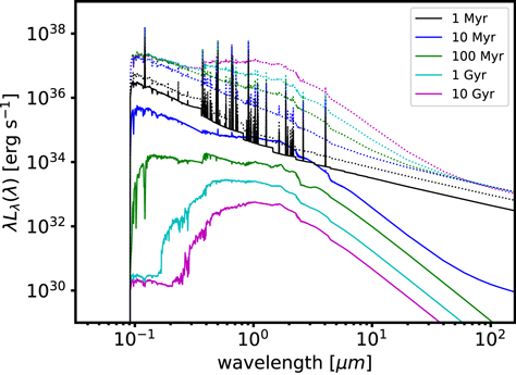
Figure 3. Stellar and gas emission spectra generated by stellar population model PEGASE. The solid lines show models with instantaneous star formation (with decreasing luminosity as age increases), while the dotted lines show models with constant star formation (with increasing luminosity as age increases). Here we normalize the instantaneous star formation models to  and constant star formation models to
  . These models use solar metallicity and have gas emission (continuum and lines) added.
Download figure:
Standard image High-resolution imagePEGASE uses the isochrone synthesis method, which integrates an IMF, evolutionary tracks, and a library of stellar spectra, to produce the integrated SEDs of a stellar population. In a single star formation event, the IMF describes the relative abundance of newly formed stars of different masses. We used the Salpeter (1955) IMF from 0.1 to 120 M⊙. This IMF was used, as it is a common one to assume for SFR studies and one of the applications of the DirtyGrid is to investigate the various SFR recipes. Kroupa (2001) has found variation in the IMFs between globular clusters and the Galactic-field, but it is uncertain how or whether the IMF change in different environments and redshifts. Adopting a cutoff in the low mass range of the IMF can lead to a factor of ∼1.5 change in the SFR determined from empirical SFR indicators (Kennicutt & Evans 2012).
The evolutionary tracks describe the trajectory of stars in the Hertzsprung-Russell diagram. PEGASE mainly uses tracks from the Padova group, but they also supplemented the Padova tracks in a number of special evolutionary phases. Most importantly, they use the equations from Groenewegen & de Jong (1993) to create pseudo-tracks for the thermally pulsing asymptotic giant branch (TP-AGB) stars, which are short-lived but luminous.
In general, the SFR of a galaxy is a function of time. The typical timescale for gas depletion is about 3 Gyr (Pflamm-Altenburg & Kroupa 2009), so it is reasonable to expect the SFR to decrease over time. The time-dependent profile of star formation can be modeled as an exponentially decaying burst (Searle et al. 1973; Conti et al. 2003). However, given limited computational resources, we choose to model only the following two extreme cases: instantaneous burst and constant star formation, which correspond to time constants of infinity and zero, respectively. These two cases bracket the possible real world scenarios. For example, the fraction of young stars in an exponentially decaying star formation model is lower than that of a constant star formation model, and higher than an instantaneous burst model, for any finite decaying time constants. Our choice reduces the "star formation history" dimension of our parameter grid to only two points. With further increase in the capability of supercomputers and more data to constrain the parameter space, we may include exponentially decaying star formation into a future version of DirtyGrid, potentially increasing the number of points in the "star formation history" dimension by an order of magnitude.
Closely related to the star formation history is the age of the stellar population. The age of the stellar population reflects the time elapsed since the "instantaneous" burst of start formation in the case of a burst model, or the time over which the model has been forming stars at a constant rate. To cover a range of plausible ages for the stellar populations, the DirtyGrid includes both burst and constant stellar populations with ages between 1 Myr and 13 Gyr.
The integrated SED of a stellar population depends on the initial metallicity of the stellar population. Populations with different metallicity trace different evolutionary tracks and populate different isochrones. Hence population synthesis models, including PEGASE, also specify the metallicity of the stellar population. To cover a realistic range of integrated galactic metallicities, in DirtyGrid we compute SEDs for stellar populations spanning a range of metallicities between Z of 0.0001 and 0.1, where solar metallicity is ∼0.013.
To control the intensity of stellar emission, we scale the input SED by the stellar surface density. For instantaneous star formation (ISR) models, the scaling factor is the stellar mass surface density  . For constant star formation (CSR) models, the scaling factor is the SFR surface density
  . The total mass of stars formed in CSR models is the product of
  and the age of the stellar population. In both cases, the final stellar mass depends on the evolution of the stellar population, which is an output of PEGASE, and due to the finite life time of stars is always smaller than the total mass of stars formed. We choose the range of stellar mass or SFR by comparing the model outputs to SINGS (Kennicutt et al. 2003) and LVL galaxies (Dale et al. 2009) and star formation regions in very nearby galaxies. The range we use covers the range derived empirically from these observations.
DIRTY does not calculate the radiative transfer through gas, which would add significant complexity to the code. The effect of gas, which is particular important for young stellar populations due to the significant UV radiation, is approximated by a gaseous nebula that is local to the stars and optically thick in the Lyman lines. Under extremely intense UV radiation, the absorption rate of Lyman continuum photons by gas is limited by the number of neutral hydrogen atoms, so some of these photons should be absorbed by dust instead. In contrast, in our models these photons are always absorbed by gas. The difference is negligible in typical H ii regions (Walcher et al. 2011). We add the gas continuum and recombination lines emission, as calculated by PEGASE, to the stellar emission.
The combined spectrum at a given age, star formation history, metallicity, and intensity defines the radiation sources used as input for the DIRTY radiative transfer model.
2.3. Dust
The dusty medium through which source photons propagate in a radiative transfer simulation has a profound effect on the output spectrum of the simulation. The optical depth, albedo, and scattering phase function of the dust determines the probability that a photon will interact, as well as the amount of the source energy that is absorbed or scattered. Once absorbed, the radiation is thermalized and re-emitted according to the emission cross sections of the dust population, producing a dust emission spectrum.
To integrate the dust population into the radiative transfer simulation, a dust grain model is required. A dust model specifies the composition, size distribution, and micro-physics (e.g., the optical properties) of the dust grain population. Since the DirtyGrid is designed to provide a grid of SEDs representative of the integrated SED of galaxies over a wide range of galactic parameters, the dust inputs must reflect the range of dust characteristics observed in galaxies. Therefore, with DirtyGrid, we adopt the dust grain models described in Weingartner & Draine (2001), who used an analytical expression to parametrize the size distributions of "astronomical" carbonaceous and silicate grains. We summarize the Weingartner & Draine (2001) models we use and refer the interested reader to that paper for the details. They fit the extinction curves of sightlines in the MW, Large Magellanic Cloud (LMC), and Small Magellanic Cloud (SMC) to produce sets of best-fit parameters of the size distributions. For the MW, we pick the RV = 3.1,  model; for LMC, we choose the
  model of the "LMC 2" environment (Meaburn 1980; Misselt et al. 1999, the supergiant shell on the southeast side of 30 Dor); for SMC we take the model of the "SMC bar" environment (Gordon & Clayton 1998), which is the only model presented for the SMC. The grains are spherical, and their radii range from 3.5 Å to 2.5 μm. The spherical grain approximation enables the use of Mie theory to compute the optical scattering and absorption cross sections. The silicate grains use the same properties for all grain sizes, unlike the carbonaceous grains. The smallest carbonaceous grains have PAH properties, the largest grains have graphite properties, and intermediate sizes have properties that are a mixture of the two. By including MW, LMC, and SMC dust grain models in the DirtyGrid, our SEDs represent the full range of dust properties that have been observed in galaxies. Figure 4 gives the extinction curves for the three different models of dust grains used in the DirtyGrid.
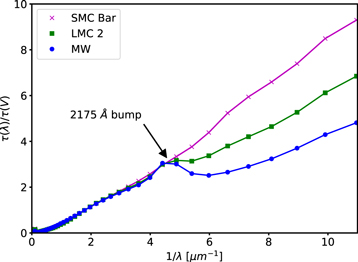
Figure 4. DirtyGrid extinction curves for the MW, LMC 2, and SMC Bar dust models are shown. The primary differences between these curves are the strength of the 2175 Å bump and the far-UV rise. Our choice of dust types is intended to cover the range of dust properties observed in galaxies.
Download figure:
Standard image High-resolution imageThe radiative transfer routine in DIRTY calculates the total energy absorbed by dust in each of the grid cells in our local mean intensity storage grid. DIRTY then launches the dust emission routine to calculate the emission spectrum in each grid cell independently (and sequentially). For each species of dust grain (carbonaceous and silicate), starting at the smallest grain size, we calculate the stochastic heating of dust grains. The calculation of stochastic heating is computationally expensive, but various authors (e.g., Leger & Puget 1984) have shown that stochastic heating is needed to explain the near/mid-IR emission in excess of that expected from dust in pure thermal equilibrium in many astronomical systems. Using the method of Guhathakurta & Draine (1989), we populate a matrix with the probabilities of transitions between different internal energy states, each of which has an associated temperature. The solution of the transition matrix gives us the probability of finding the dust grain in each of the states, P(T). The emission at this particular grain size is an integration of the modified blackbody function (taking into account the effects of the changing emissivity across wavelengths) weighted by P(T). As the calculation moves to grains of increasing sizes, we reach a regime in which the grains are in equilibrium with the radiation field and P(T) becomes strongly peaked. At this point we switch over to the simpler equilibrium heating calculation, in which grains emit in a modified blackbody function with a single temperature. We find the equilibrium temperature, and therefore the equilibrium emission as a function of wavelengths, by simply balancing the energy absorbed and emitted by dust grains of this particular size. In the end, we sum over the emission from all grain sizes and species to obtain the total dust emission spectrum in the current grid cell. A rigorous discussion on dust modeling in DIRTY is available in Misselt et al. (2001). Recently, Camps et al. (2015) compared the dust emission algorithms of six radiative transfer codes, including our latest code, and found the all six codes consistent within 10%.
In addition to the physics that describes how photons will interact with dust and how the dust will respond to the input of energy, the total amount of dust in the model must be specified. Rather than directly specifying the mass of dust, in the DirtyGrid, the optical depth at V band ( ) is specified as an input parameter to DIRTY.
  is measured from the center of the model to the edge, averaged over all
  steradians of solid angle. For normal disk galaxies, Holwerda et al. (2007) has found that
  is on the order of unity. Dale et al. (2006) also found that the average attenuation is
  (i.e.,
  ) for a large portion of SINGS galaxies. In the DirtyGrid, the
  dimension in the parameter space span over 2 dex of optical depths from 0.1 to 10, which we believe is sufficient to cover the majority of observed galaxies.
2.4. Geometry
In the DIRTY model, the global geometry describes the relative distributions of dust and stars, while the local geometry determines the clumpiness of dust. Geometry has a profound effect on radiative transfer, both on the attenuation (e.g., by providing paths of different optical depths) and the emission (e.g., through the non-trivial spatial and temperature distribution of dust). While an extinction curve can be accurately measured by comparing the spectrum of a reddened and an unreddened star of the same spectral type (and has been done for sightlines in the MW, LMC, and SMC), in the complex geometries generally associated with galactic environments, only "attenuation" curves can be measured. A dust attenuation curve is defined as the wavelength dependence of attenuation by dust, including the effects of absorption, scattering out of the beam, and scattering into the beam, and is usually measured for regions of galaxies or whole galaxies. In contrast to the traditional extinction curve, determination of attenuation curves is more challenging because it is difficult to independently constrain the underlying stellar populations and radiative transfer effects (anisotropic scattering, differential extinction between sources, dust exposed to different radiation field intensities, and dust clumpiness). Baes & Dejonghe (2001) found that scattering approximations such as isotropic scattering can be a major source of error in radiative transfer. Even in the absence of scattering, Disney et al. (1989) found that the choice of model geometry significantly affects attenuation.
Commonly used global geometries for radiative transfer modeling of galactic environments include plane-parallel slabs, spheres, double-exponentials, and arbitrary distributions (see Calzetti 2001 and references therein). Plane-parallel slabs are simplest to model, but Calzetti et al. (1994) found that such a model does not agree with the UV-optical spectra of starburst galaxies, and they empirically calibrated a single attenuation curve of starburst galaxies as a third-degree polynomial in  . To account for that fact that young stars are likely to be embedded in their birth cloud and therefore more attenuated then old stars, Silva et al. (1998) and Charlot & Fall (2000) created models that provide additional opacity around the young stars.
In the DirtyGrid, we use the Cloudy, Dusty, and Shell global geometries, as defined by Witt & Gordon (2000), that are described below. These geometries are spherically symmetric and efficient for radiative transfer. DIRTY supports arbitrary stellar and dust geometries, and we implement the dust geometries as spatially resolved blocks in our local mean intensity storage grid, which has a resolution of 30 × 30 × 30. As we embedded these spherical geometries in a cubical grid, the grid cells outside the sphere are empty and explicitly not traversed during the radiative transfer calculation. A visualization of the cross section of the geometries is shown in Figure 5. In the Cloudy geometry, stars are uniformly distributed in the sphere, and a dusty core is located within 0.69 times of the system radius. In the Dusty geometry, stars and dust are uniformly distributed in the sphere. In the Shell geometry, stars extend only to 0.3 times of the system radius and are surrounded by a shell of dust from 0.3 to 1.0 times of the system radius. Witt & Gordon (2000) found that a Shell geometry (with clumpiness) with  can reproduce the Calzetti Attenuation Law (Calzetti et al. 1994; Calzetti 1997).
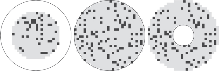
Figure 5. 2D cross sections of the Cloudy, Dusty, and Shell geometries. The darkness of the squares schematically indicates the density of dust in that area. For clumpy models, the density ratio is 100 (i.e., clumps have 100 times the density of the diffuse medium), while for homogeneous models, the density ratio is 1 (i.e., the same density for gray and black squares). The stellar population is uniformly distributed inside the smooth circle.
Download figure:
Standard image High-resolution imageIn addition to global geometry effects, dust clumpiness is also important. For a given mass of dust, clumpiness reduces the overall opacity and therefore the efficiency of dust in converting UV-optical radiation into IR. Popescu et al. (2000) found that while a single exponential diffuse dust disk can reproduce the optical and NIR emission, a clumpy distribution of dust that is spatially correlated with stars is needed to account for the FIR and sub-mm emission. Duval et al. (2014) found that a clumpy and dusty ISM appears more transparent to radiation (both line and continuum) compared to an equivalent homogeneous ISM of equal dust optical depth. Witt & Gordon (1996) found that a minimum of two phases of non-zero density is necessary to model the interstellar dust medium in the MW. In our clumpy models, we use a two-phase medium with a filling factor of 15% and a density ratio of 100 to implement clumpiness; Witt & Gordon (1996) found that these values reproduce the cloud mass spectrum and fractal dimension of the diffuse clouds in the MW. For comparison, we also run homogeneous models, which is equivalent to setting the density ratio to unity.
While spherical geometries are efficient for computation, they may not represent the realistic geometries of whole galaxies. For example, Baes et al. (2003) modeled spiral galaxies with double exponential disks, which more closely resembles spiral galaxies than our spherical models. Realistic geometries are suitable for studying individual objects, as they can provide spatial images and in principal reproduce detailed features better. However, they are not suitable for DirtyGrid because the radiative transfer in such geometries would take many orders of magnitude longer to compute, and the broadband SED may not contain sufficient information to constrain the additional parameters. Instead, we use simplified geometries to span the possible range in galactic environments. For the same amount of dust, the Shell geometry provides the highest efficiency in attenuation and is similar to the birth cloud of young stars, while the Cloudy geometry gives the lowest attenuation and is similar to the environments in elliptical galaxies or the bulge of spiral galaxies. In essence, we model pieces of galaxies, and in the approximate limit where the global UV–IR SEDs of galaxies are dominated by a few representative types of non-interacting pieces, we can use a combination of models to fit the global SEDs. Within a single stellar population, we do not segregate the stars by age and place young stars in more embedded dust. However, we can approximate the segregation by combining the outputs of two models of different stellar ages, with the younger model having a higher optical depth than the older model.
In the DirtyGrid, the stellar mass and the radius of the spherical geometry (the model size) are degenerate parameters. We use the same ratio of the clump size to the model size for all models. In each grid cell, the dust emission spectrum is calculated from the dust absorption spectrum. At each wavelength, the amount of energy absorbed depends on the radiation intensity. As we increase the model size (and therefore the grid cell size) by a factor of x, the radiation intensity in each cell drops by a factor of x2. A corresponding increase in the stellar mass by a factor of x2 restores the radiation intensity to the original level. The output SED will have the same shape but scaled up by a factor of x2. Effectively, stellar mass per radius squared, essentially the mass surface density, determines the SED shape. Ivezic & Elitzur (1997) have a rigorous derivation of the scaling behavior in radiation transfer. In practice, we run all models with a 10 kpc radius and scale the output as needed.
3. Populating the Parameter Space
The parameter space of the DirtyGrid has eight dimensions: global geometry, stellar age, metallicity, stellar scaling factor, star formation type (burst/constant), amount of dust, dust clumpiness, and dust grain type. The range of input parameters is discussed in in Section 2 and summarized in Table 1. Given the large parameter space, care in the sampling strategy can significantly reduce the resources needed to generate the grid. Among these eight dimensions, we treat stellar age, stellar mass (through the stellar mass or SFR surface density; see Section 2.2), and amount of dust as continuous variables because we are interested in deriving accurate values of these variables from SED fitting. We attempt to fully resolve the dependence of the broadband SEDs on the continuous variables while being conservative on the number of samples required. We designate the other five dimensions as discrete variables and bracket the possible range with a small number of samples, reducing the computation needed at the expense of the ability to derive accurate intermediate values.
Table 1. Dimensions and Ranges of the Parameter Grid and the Number of First Stage Samples
| Parameter | Range | #Samples |
|---|---|---|
| Continuous Variables | ||
| Stellar Age | 1 Myr–13 Gyr | 14–28 |
| Stellar Mass | (depends on SF Type) | 15 |
| Amount of Dust |

|
7 |
| Discrete Variables | ||
| SF Type | burst/constant | 2 |
| Metallicity | Z = 0.0001–0.1 | 5 |
| Global Geometry | Cloudy/Dusty/Shell | 3 |
| Local Geometry | homogeneous/clumpy | 2 |
| Grain Type | MW/LMC/SMC | 3 |
Note. The number of models in the first and second stages are 365 K and 225 K, respectively. With an average run time of ∼10 hr, the grid used ∼5M CPU hours. The first three parameters are continuous variables and subject to non-uniform sampling and interpolation.
Download table as: ASCIITypeset image
Among the discrete dimensions, we have three grain types, MW, LMC, and SMC, based on the Weingartner & Draine (2001) models (Section 2.3); three global geometries, Cloudy, Dusty, and Shell, based on the Witt & Gordon (2000) geometries (Section 2.4); two local geometries, homogeneous and clumpy, the latter of which is based on the filling factor and density ratios in Witt & Gordon (1996; Section 2.4); two types of star formation history, burst and constant (Section 2.2); and five values of metallicities. Each of these could be easily expanded into a full continuous dimension (e.g., one could define different levels of clumpiness), but this would greatly increase the amount of computation needed. Among the five discrete variables, metallicity could be the most interesting one to expand into a continuous dimension, but our preliminary results show that UV–IR SED fitting typically cannot constrain metalliticity to high accuracy, so we only selected the discrete absolute metallicity values of Z = 0.0001, 0.0004, 0.004, 0.02, and 0.1, where the Padova evolutionary tracks are available, thereby removing the need to interpolate the tracks.
For the three continuous variables, we adopt a 2-stage sampling strategy. Because of the high number of samples in these three dimensions, running all combinations of samples that are required to fully resolve each of these three dimensions independently is computationally expensive. Since the rate of change of broadband fluxes may depend on which part of the parameter space we are in, a non-uniform sampling of these three dimensions can greatly reduce the number of models needed. We can then interpolate the broadband fluxes over the missing samples, where the rate of change with respect to the interpolating variables is slow or constant. The first stage sampling involves a mostly uniform grid (except in the stellar age dimension), and the selection is guided by a high resolution study of the dimensions in a limited parameter space. Table 1 provides a summary of the first stage sampling. Based upon the observed behavior in the first stage, the second stage sampling involves filling in more models around grid points where the SED changes rapidly, and is non-uniform.
3.1. First Stage Sampling
Prior to running the first stage sampling, we ran a pilot grid with high resolution in each of the three continuous variables (stellar age, stellar mass, and amount of dust) to study the behavior of the SEDs as a function of these variables. We found that the band fluxes vary smoothly as a function of optical depth. While the precise details of the output spectrum are sensitive to the parameters, the band integrated fluxes (e.g., using the Johnson UBVRI band pass filters) are far less sensitive. This allows us to sample optical depths sparsely and then interpolate over intermediate optical depths to get band fluxes at the intermediate values. Note that the first stage sampling does not have to be precise, because the second stage sampling fills in where the sampling is insufficient in the first stage.
Figure 6 shows that the optical V band fluxes vary smoothly over two dex of optical depth (from  = 0.1 to 10.0). To quantitatively measure the error interpolation introduces, we ran the model with 25 different optical depths and selected stellar ages and geometries with all other parameters fixed (solar metallicity, instantaneous star formation, and clumpy MW dust). The 25 different values are logarithmically evenly spaced between
  = 0.1 and 10. Then we take 1 model from every 4 models, resulting in 7 (including the ones on the edge) models sparsely sampling the optical depth. From these 7 models we calculate the band fluxes, and use linear interpolation (in log space) to predict the band fluxes at the intermediate optical depths, and finally compare the interpolated fluxes and actual fluxes. For the limited parameter space we looked at, they generally agree within 1%. The behavior for stellar mass is also smooth, and we choose to use only 15 samples to span over 7 dex of stellar mass values, including the edge points.
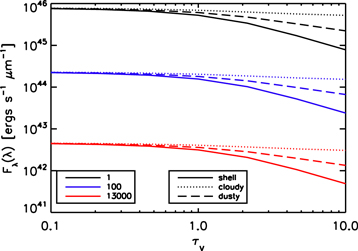
Figure 6. Optical V band flux vs. optical depth for three stellar ages (1, 100, and 13,000 Myr) and three clumpy geometries (Shell, Dusty, and Cloudy). In general, band integrated fluxes vary smoothly with optical depth. The smoothness enables the use of interpolation to greatly reduce the number of optical depths needed.
Download figure:
Standard image High-resolution imageThe behavior of stellar ages, however, requires many more samples to resolve. For the purpose of the first stage sampling in stellar age, we study the band integrated fluxes of the unreddened spectra of stellar populations, which do not require radiative transfer. In Figure 7, we plot the V band fluxes against the full range of stellar ages, sampled at 47 points. Between 10 Myr and 13 Gyr, the age samples are roughly evenly spaced in log space (12 per dex), but below 10 Myr we included all integer multiples of Myr because PEGASE does not output results at fractional Myr ages. Having a constant amount of young stars and a steadily increasing amount of old stars, the constant star formation models give a much smoother curve. On the other hand, instantaneous star formation models exhibit relatively sharp changes in V band fluxes as they evolve. This is due to evolved stars entering rapidly changing phases or the death of luminous stars. In order to achieve <10% accuracy in band fluxes, we find that we need 14 samples of ages for constant star formation models, but the number for instantaneous star formation models is much higher and depends on the metallicity.
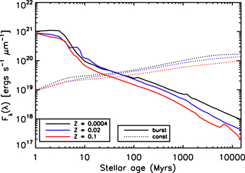
Figure 7. Unreddened optical V band flux vs. stellar age for three absolute metallicities and the two types of star formation (burst and const). While the behavior is smooth for constant star formation models (const), the changes are quite abrupt for instantaneous star formation models (burst), especially between 1 and 10 Myr. As such, we spent more computational resources for the burst models. Note that the burst models show different features for different metallicities.
Download figure:
Standard image High-resolution imageTo pick the minimum number of samples needed to reach 10% error due to age interpolation in burst models, we did an exhaustive search for the optimal set for each metallicity. From 10 Myr to 10 Gyr, we divided the range of age into 6 equal segments (in log space). For example, the first segment goes from 10 to 32 Myr. In each segment, we have five possible sample locations that are uniformly distributed. At each location, the sample is either present or absent. For each of the  combinations, we compute the band integrated fluxes and interpolate the fluxes at the missing samples. We compare the interpolated fluxes with the correct fluxes to get the fractional error. With a error target of <10%, we pick the minimum number of samples needed in each segment and arrive at a list of selected ages. We run the age selection algorithm for different star formation types and metallicity separately. Figure 8 shows our age selection for models with instantaneous star formation from 10 Myr to 10 Gyr. The number of age samples for burst models ranges from 22 to 28.
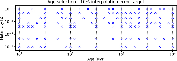
Figure 8. Non-uniform age selection for models with instantaneous star formation. The blue points indicate our age samples (horizontal axis), which depend on the metallicity. The vertical dotted lines indicate age values that we always sample (2 per dex). We choose them using an algorithm that picks the minimum number of points to achieve <10% interpolation error in all bands. Note that while this figure shows the results for seven metallicities available in the Padova tracks for completeness, we only use five of them in the DirtyGrid.
Download figure:
Standard image High-resolution image3.2. Second Stage Sampling
We improve upon the first stage sampling by filling in models at locations with insufficient interpolation accuracy. Because of possible nonlinearity in the SED landscape, we cannot determine the error in the interpolated fluxes at locations of the parameter space that we have not sampled. Even in rapidly changing areas, the interpolated fluxes could be accurate if the changes are smooth. As an estimate of the interpolation accuracy, we again compared the actual band fluxes of each model with the interpolated band fluxes using the nearby points. Above a threshold of error (15%), we fill in more samples around such models. To choose the second stage samples, we apply the following procedure for each of the three continuous dimensions (denoted as x):
- 1.Loop over each samples in the grid, except the ones with the maximum or minimum allowed values of x.
- 2.While ignoring the current sample, interpolate the broadband fluxes between the model that has a higher value of x and the model that has a lower value of x.
- 3.Compare the broadband fluxes of the current sample with the interpolated fluxes.
- 4.If the error in any of the bands is greater than 15%, include the two neighboring grid points of the current sample (in the x dimension) in the second stage sampling.
We calculate the error of the interpolated fluxes, assuming that the actual model has the true values. The procedure identified 225K locations to fill in second stage samples. In the final DirtyGrid, we interpolate over the parameter space using the combined set of first and second stage samples.
4. Results
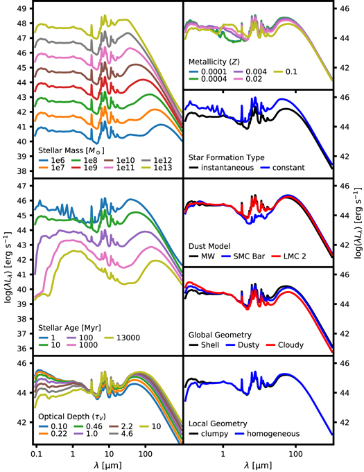
The panel of plots in Figure 9 illustrates the dependence of the model output spectra on the model input parameters. The scale of each plot is the same to show how the amplitudes of change of the parameters compare to each other. When all other parameters are held constant, an increase in the stellar age reddens the UV-optical spectra and decreases the total stellar luminosity, due to the death of luminous and UV-bright stars. Both of these effects decrease the average dust temperature and shift the peak of the dust emission in the far-IR to a longer wavelength. The oscillations at optical wavelengths for the 1 Myr model are due to the existence of strong nebular emission lines and our relatively low resolution wavelength grid that does not resolve the lines. This is acceptable because the change in the broadband fluxes due to the dust radiative transfer does not depend sensitively on the precise wavelength of the gas emission lines. Since the total amount of input radiation scales with stellar mass, the stellar mass plot shows the greatest change in the level of output flux. A higher stellar mass also results in higher dust temperature. Stellar metallicity correlates with the UV radiation field hardness and therefore the total amount of dust emission. Its effect on the intrinsic near-IR colors are prominent in the output spectra. In the star formation type plot, we compare an instantaneous star formation model to a continuous star formation model with the same total stellar mass formed. While both models have a 10 Myr stellar population age, the latter spectra resembles a 1 Myr instantaneous star formation model but with a lower fraction of energy in the emission lines. Optical depth determines how much energy is absorbed in the UV-optical and re-emitted into the IR, so it is the primary driver behind changes in the IR to UV ratio. The values are shown in the legend in the dust extinction optical depth at V band ( ). The attenuation optical depth at V band (
 ), which includes the radiative transfer effects, also depends on the geometry. The Shell geometry gives the highest attenuation, followed by Dusty and Cloudy. The effect of changing the geometry from Cloudy to Shell is similar to increasing
  , except that in the former case the dust temperature increases, while in the latter it decreases. Dust clumpiness has a lesser effect on the overall attenuation, but the change in attenuation at extreme UV wavelength is significant. Finally, the choice of dust grain model also affects the attenuation curve, but the most prominent effect is the strength of the PAH emissions around 8 μm. The MW dust grain model has the highest PAH fraction, followed by LMC and SMC, and this is reflected in the fraction of energy emitted at around 8 μm.
Figure 9. Example DIRTY model output spectra showing the variations in each dimension of the parameter grid. In each plot, we vary one parameter and fix all the others. The fixed parameter values are 10 Myr old stellar age, 1010 solar masses, solar metallicity, instantaneous star formation,  , Milky Way type dust, shell geometry, 10 kpc radius, and clumpy dust, except when shown in the legend of each plot.
Download figure:
Standard image High-resolution image
In order to fit these model spectra to broadband SEDs of real galaxies, we need to compute the fluxes that various instruments would measure if they were to observe the hypothetical models as an object on the sky. The conversion from model spectra to broadband luminosities require the use of band pass filters of each instrument, also known as filter response functions. We integrate the DirtyGrid spectra multiplied by the band pass filters of GALEX FUV/NUV, Johnson UBVRI, SDSS ugriz, 2MASS JH , Spitzer IRAC/MIPS, and Herschel PACS/SPIRE (Engelbracht et al. 2007; Gordon et al. 2007; Stansberry et al. 2007; Hora et al. 2008). We then interpolate the broadband luminosities in the stellar age, stellar mass, and optical depth parameter to arrive at a regular eight-dimensional cube of luminosities in each band, using linear interpolation in log space. We present the resultant broadband SEDs at 10.5281/zenodo.121427 in HDF5 format. A few SEDS are shown in Table 2 as an example.
Table 2. Band Integrated Luminosities of DIRTY Models in the GALEX, SDSS, Johnson Optical/near-IR, Spitzer IRAC/MIPS, and Herschel SPIRE Bands
| Model ID | Geometry | Dust Type | Stellar Age | Metallicity | SF Type |

|
Stellar Mass |
|---|---|---|---|---|---|---|---|
| GALEX/FUV | GALEX/NUV | SDSS/u | SDSS/g | SDSS/r | SDSS/i | SDSS/z | |
| U | B | V | R | I | |||
| J | H | K | IRAC1 | IRAC2 | IRAC3 | IRAC4 | |
| MIPS24 | MIPS70 | MIPS160 | SPIRE250 | SPIRE350 | SPIRE500 | ||
| AB2820 | homo/cloudy | SMC | 1 | 0.004 | burst | 10 | 1.0E+8 |
| 4.59E+44 | 1.71E+44 | 9.64E+43 | 6.05E+43 | 2.95E+43 | 2.75E+43 | 1.60E+43 | |
| 9.56E+43 | 5.27E+43 | 5.15E+43 | 3.26E+43 | 1.13E+43 | |||
| 3.35E+42 | 1.18E+42 | 8.23E+41 | 2.80E+41 | 2.55E+41 | 1.92E+41 | 2.37E+41 | |
| 1.66E+41 | 2.68E+41 | 5.51E+41 | 1.93E+41 | 5.47E+40 | 1.16E+40 | ||
| AB2823 | homo/cloudy | SMC | 100 | 0.0004 | burst | 0.464159 | 1.0E+8 |
| 1.27E+43 | 6.94E+42 | 3.70E+42 | 3.44E+42 | 1.78E+42 | 1.09E+42 | 7.19E+41 | |
| 3.76E+42 | 3.87E+42 | 2.37E+42 | 1.56E+42 | 9.17E+41 | |||
| 3.19E+41 | 1.46E+41 | 5.43E+40 | 1.00E+40 | 4.15E+39 | 2.33E+39 | ||
| 2.44E+39 | 1.44E+39 | 1.11E+39 | 2.98E+39 | 2.03E+39 | 8.11E+38 | 2.19E+38 | |
| AB2883 | homo/cloudy | SMC | 100 | 0.02 | burst | 10 | 1.0E+8 |
| 5.07E+42 | 3.01E+42 | 1.93E+42 | 1.96E+42 | 1.17E+42 | 8.20E+41 | 6.92E+41 | |
| 1.96E+42 | 2.15E+42 | 1.45E+42 | 1.05E+42 | 7.49E+41 | |||
| 5.04E+41 | 3.52E+41 | 1.63E+41 | 3.68E+40 | 1.67E+40 | 8.07E+39 | ||
| 3.89E+39 | 1.02E+39 | 8.10E+38 | 2.18E+39 | 3.48E+39 | 2.57E+39 | 1.12E+39 | |
| AB2887 | homo/cloudy | SMC | 13000 | 0.02 | burst | 1 | 1.0E+8 |
| 7.31E+38 | 7.88E+38 | 9.67E+39 | 3.27E+40 | 4.44E+40 | 4.42E+40 | 4.53E+40 | |
| 1.03E+40 | 2.73E+40 | 4.15E+40 | 4.43E+40 | 4.48E+40 | |||
| 3.34E+40 | 2.33E+40 | 9.93E+39 | 1.96E+39 | 7.88E+38 | 3.29E+38 | 1.08E+38 | |
| 3.10E+36 | 1.17E+36 | 1.29E+36 | 3.85E+36 | 6.26E+36 | 6.03E+36 |
Note. All luminosities are in  , stellar age is in Myr, and stellar mass is in
  . The lines are wrapped for display purposes. The full table is available at 10.5281/zenodo.121427 in HDF5 format.
Download table as: ASCIITypeset image
After the completion of the grid, we run 30,000 models at randomly selected locations in the parameter grid. We then compare their integrated band fluxes to the interpolated fluxes obtained from the grid without these additional 30,000 models. The typical error introduced by interpolation is ∼3%. The largest interpolation error (∼10%) comes from the FUV band of evolved stellar populations. In instantaneous star formation models, the FUV rapidly decreases as the stellar population ages, and our sampling of stellar age in the DirtyGrid is not sufficient to resolve the detailed behavior in FUV. The same issue affects the NUV to a lesser extent. This is usually not a problem because the FUV flux in normal star-forming galaxies is dominated by young populations, but it could result in reduced constraining power of the FUV band in fitting elliptical galaxies or galaxies that primarily contain evolved stellar populations.
5. Summary
We describe how we constructed the DirtyGrid, a grid of models of UV to IR/sub-mm SEDs of dusty stellar populations. This serves as the foundation for later work, where we will use combinations of these models to study the dust properties and the accuracy of SFR indicators in nearby galaxies. Beginning with intrinsic stellar and gas spectra from the stellar population model PEGASE, the radiative transfer model DIRTY self-consistently computes the absorption, scattering, and re-emission of dust grains. We use the MW, LMC, and SMC dust grain models in Weingartner & Draine (2001) with simplified geometries that simulate galactic environments. We explained how we chose the parameters—wide enough to cover the possible physical range, and dense enough to achieve the desired accuracy while keeping the computation manageable. The landscape of the output SED is not uniform, with more rapid changes in some part of the parameter space and less in others, which inspired our use of a two-stage sampling strategy. We present a few example SEDs in this paper, and the full set is available at 10.5281/zenodo.121427.
In addition, a python package to retrieve SEDs from this table is under development.6 By adding more realistic dust grain physics and physically connecting the UV-optical to the IR/sub-mm, these SEDs represent a clear step forward in the current state-of-the-art modeling of dust and stellar populations.
This project is supported by the NASA ADAP grant 11-ADAP11-0112, "Dusty Spectral Energy Distributions of Star Formation in Nearby Galaxies." We would like to thank the Extreme Science and Engineering Discovery Environment (XSEDE), the NASA Advanced Supercomputing (NAS) facility, and the NASA Center for Climate Simulation (NCCS) for providing their computational resources. Without these resources, this project would not be possible.