


Abstract
We present a multi-wavelength photometric catalog in the COSMOS field as part of the observations by the Cosmic Assembly Near-infrared Deep Extragalactic Legacy Survey. The catalog is based on Hubble Space Telescope Wide Field Camera 3 (HST/WFC3) and Advanced Camera for Surveys observations of the COSMOS field (centered at R.A.:  , Decl.:
 ). The final catalog has 38671 sources with photometric data in 42 bands from UV to the infrared (
 ). This includes broadband photometry from HST, CFHT, Subaru, the Visible and Infrared Survey Telescope for Astronomy, and Spitzer Space Telescope in the visible, near-infrared, and infrared bands along with intermediate- and narrowband photometry from Subaru and medium-band data from Mayall NEWFIRM. Source detection was conducted in the WFC3 F160W band (at 1.6 μm) and photometry is generated using the Template FITting algorithm. We further present a catalog of the physical properties of sources as identified in the HST F160W band and measured from the multi-band photometry by fitting the observed spectral energy distributions of sources against templates.
Export citation and abstract BibTeX RIS
1. Introduction
The Cosmic Assembly Near-infrared Deep Extragalactic Legacy Survey (CANDELS: PI. S. Faber and H. Ferguson; see Grogin et al. 2011 and Koekemoer et al. 2011) is the largest Multi-Cycle Treasury program ever approved on the Hubble Space Telescope (HST), with more than 900 orbits, and it was designed to use deep observations by the Wide Field Camera 3 (WFC3) and Advanced Camera for Surveys (ACS) instruments to study galaxy formation and evolution throughout cosmic time in five fields in many different bands. The observations were done by the HST/WFC3 as the main mode with ACS observations in parallel. The CANDELS images are publicly available, and multi-wavelength photometric catalogs are made available by the CANDELS team following the release of the images. All CANDELS photometric catalogs were selected based on the WFC3 F160W band and this is the reference image for all the other HST and non-HST data. This provides a data set with consistent photometry and physical properties across all the fields targeted as part of the survey. The CANDELS catalogs for the first two observed fields of UDS and GOODS-S (Galametz et al. 2013; Guo et al. 2013) are already publicly available31 and the three fields of COSMOS (this work), EGS (M. Stefanon et al. 2017, in preparation), and GOODS-N (G. Barro et al. 2017, in preparation) are in progress. The CANDELS observations are aimed at achieving several major science goals that could only be attained with data at the depth and resolution of CANDELS. These include studying the most distant objects in the universe at the epoch of reionization in the cosmic dawn (e.g., Finkelstein et al. 2012a; Grazian et al. 2012; Yan et al. 2012; Lorenzoni et al. 2013; Oesch et al. 2013; Duncan et al. 2014; Bouwens et al. 2015; Caputi et al. 2015; Finkelstein et al. 2015; Giallongo et al. 2015; Mitchell-Wynne et al. 2015; Roberts-Borsani et al. 2016; Song et al. 2016), understanding galaxy formation and evolution during the peak epoch of star formation in the cosmic high noon (e.g., Bell et al. 2012; Bruce et al. 2012; Kocevski et al. 2012; Lee et al. 2013; Wuyts et al. 2013; Barro et al. 2014; Hemmati et al. 2014, 2015; Whitaker et al. 2014; Williams et al. 2015), and studying star formation from deep UV observations and cosmological studies from supernova observations (e.g., Jones et al. 2013; Teplitz et al. 2013; Rodney et al. 2014, 2016; Strolger et al. 2015). These main science goals are described in more detail by Grogin et al. (2011) and Koekemoer et al. (2011).
One of the major goals of modern observational cosmology is to study the formation and evolution of galaxies with cosmic time. Recent advances in this frontier have been enabled by the availability of observations in different wavelengths, targeting different populations of galaxies (e.g., York et al. 2000; Wolf et al. 2003; Bell et al. 2004; Giavalisco et al. 2004; Skrutskie et al. 2006; Faber et al. 2007; Lawrence et al. 2007; Scoville et al. 2007b; Ilbert et al. 2013; Khostovan et al. 2015; Shivaei et al. 2015; Hemmati et al. 2017; Vasei et al. 2016). The advent of HST benefited many such studies by making it possible to have the deepest observations of the sky in multiple bands. In particular the installation of the WFC3 on board HST initiated a new stage for studying galaxy evolution at new extremes (McLeod et al. 2015; Oesch et al. 2016).
Galaxy populations at different look-back times range from very blue star-forming galaxies to red dusty or very old systems. Understanding the evolution of these populations relies on the availability of multi-wavelength photometric data from the bluest to the reddest bands possible. The CANDELS multi-wavelength catalogs combine the best and deepest observations by HST with the deepest ground-based observations and Spitzer Space Telescope data (Galametz et al. 2013; Guo et al. 2013). These catalogs of tens of thousands of extragalactic sources, consistently measured across many bands from  , bring a unique opportunity to study galaxy evolution.
The Cosmic Evolution Survey (COSMOS; Scoville et al. 2007b) centered at R.A.:  , Decl.:
  ) is a 2 deg2 field located near the celestial equator. It was initially picked to maximize the visibility from observatories from both hemispheres and was specifically chosen to avoid any bright X-ray, UV, or radio sources (Scoville et al. 2007b) and to be large enough for studies of large-scale structure (e.g., Scoville et al. 2007a, 2013; Kovač et al. 2010; Darvish et al. 2014, 2015b).
The COSMOS field was targeted by CANDELS in a north–south strip, lying within the central ultra-deep strip of the UltraVISTA imaging (McCracken et al. 2012) and hence also the Spitzer SEDS imaging (Ashby et al. 2013) in order to ensure the best possible supporting data at longer near-infrared wavelengths. The HST observations cover an area of  arcmin2 in the WFC3/IR with parallel ACS observations. The catalog was selected in the HST/WFC3 F160W band and has multi-band data for 38671 objects from ∼0.3 to 8 μm. These fluxes are measured consistently across all these bands and in agreement with photometry measurement techniques adopted by all CANDELS catalogs. We use the unprecedented depth and resolution provided by the HST for measuring the flux of the faintest targets across all bands. By fitting this multi-waveband information with template libraries, we also measured photometric redshift and stellar mass for each object.
The paper is organized as follow. Section 2 presents the data used to compile the catalog. Section 3 describes our photometry of the HST, Spitzer, and ground-based bands. Section 4 is devoted to data quality checks for our TFIT photometry. Physical parameter estimation using the measured photometry is presented in Section 5. In Section 6 we investigate the applications of our deep photometry on studies of high-redshift star-forming and quiescent galaxies. We summarize our results in Section 7. Throughout this paper we assume a cosmological model with  ,
,  , and
, and  . All magnitudes are in the AB system where
  (Oke & Gunn 1983).
The CANDELS COSMOS photometry catalog will be publicly available through the CANDELS Web site32 along with the physical properties estimates and all the documentations. These will also be available on the Mikulski Archive for Space Telescopes (MAST),33 via the online version of the catalog and through Centre de Donnees astronomiques de Strasbourg (CDS). We will also make these data available through the Rainbow Database34 (Pérez-González et al. 2008; Barro et al. 2011).
2. Data
The COSMOS field (Scoville et al. 2007b) has been observed in many different wavelengths from the X-ray to the far-infrared. There are observations from the CFHT/MegaPrime in the u*, g*, r*, i*, and z* (Gwyn 2012), from the Subaru/Suprime-Cam in the B,  , V,
, V,  ,
,  , and
, and  (Taniguchi et al. 2007), from the VLT/Visible and Infrared Survey Telescope for Astronomy (VISTA) in the Y, J, H, and Ks bands (McCracken et al. 2012), from Spitzer in the four IRAC bands (Sanders et al. 2007; Ashby et al. 2013), VLA (Schinnerer et al. 2007), XMM (Cappelluti et al. 2007; Hasinger et al. 2007), Chandra (Elvis et al. 2009; Civano et al. 2016), and GALEX (Schiminovich et al. 2005). There are also numerous medium- and narrowband observations available in the COSMOS from Mayall NEWFIRM (Whitaker et al. 2011) and Subaru Suprime-Cam (Taniguchi et al. 2015). The full COSMOS field has been observed with HST in F814W (Koekemoer et al. 2007) and contains more than 2 million galaxies with multi-band data from the UV to the far-IR (Capak et al. 2007; Mobasher et al. 2007; Ilbert et al. 2009, 2013). Furthermore, COSMOS has been followed up spectroscopically by the larger and most sensitive telescopes/instruments like VLT/VIMOS (e.g., Lilly et al. 2009; Le Fèvre et al. 2015) and Keck/DEIMOS and MOSFIRE among others.35
This makes it possible to study different populations of galaxies from blue and young systems at shorter wavelengths to red dusty or old objects at longer wavelengths. These ancillary data are accompanied by high-resolution observations from CANDELS using the HST in both visible and near-infrared. Figure 1 shows the transmission curves for all bands included in the CANDELS COSMOS catalog.
(Taniguchi et al. 2007), from the VLT/Visible and Infrared Survey Telescope for Astronomy (VISTA) in the Y, J, H, and Ks bands (McCracken et al. 2012), from Spitzer in the four IRAC bands (Sanders et al. 2007; Ashby et al. 2013), VLA (Schinnerer et al. 2007), XMM (Cappelluti et al. 2007; Hasinger et al. 2007), Chandra (Elvis et al. 2009; Civano et al. 2016), and GALEX (Schiminovich et al. 2005). There are also numerous medium- and narrowband observations available in the COSMOS from Mayall NEWFIRM (Whitaker et al. 2011) and Subaru Suprime-Cam (Taniguchi et al. 2015). The full COSMOS field has been observed with HST in F814W (Koekemoer et al. 2007) and contains more than 2 million galaxies with multi-band data from the UV to the far-IR (Capak et al. 2007; Mobasher et al. 2007; Ilbert et al. 2009, 2013). Furthermore, COSMOS has been followed up spectroscopically by the larger and most sensitive telescopes/instruments like VLT/VIMOS (e.g., Lilly et al. 2009; Le Fèvre et al. 2015) and Keck/DEIMOS and MOSFIRE among others.35
This makes it possible to study different populations of galaxies from blue and young systems at shorter wavelengths to red dusty or old objects at longer wavelengths. These ancillary data are accompanied by high-resolution observations from CANDELS using the HST in both visible and near-infrared. Figure 1 shows the transmission curves for all bands included in the CANDELS COSMOS catalog.
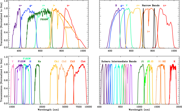
Figure 1. Transmission curves for the CFHT and ACS visible (top left), Subaru optical broadband and narrowband (top right), WFC3 and UltraVISTA near-infrared and Spitzer infrared (bottom left) and the Subaru intermediate- and NEWFIRM medium-band filters (bottom right) used in the COSMOS CANDELS TFIT catalog. These cover observations at ∼0.3–8 μm in 42 filters. The filters are adopted from http://cosmos.astro.caltech.edu/page/filterset. The effective wavelength of the filters are reported in Tables 1 and 2.
Download figure:
Standard image High-resolution image2.1. CANDELS HST Observations
The CANDELS COSMOS field was observed by the WFC3 in F125W and F160W (J125 and H160) and in parallel by the ACS in the F606W and F814W filters (V606 and i814). The WFC3 observations covered a rectangular grid of 4 × 11 tiles ( ) running north to south, allowing for maximum contiguous coverage in the near-infrared. The field was observed over two epochs with each tile observed for one orbit in each epoch. The one-orbit observations were divided into two exposures in F125W (
 orbit depth) and F160W (
 orbit depth) along with parallel ACS observations in the F606W and F814W (Grogin et al. 2011; Koekemoer et al. 2011). The exposures in each orbit were dithered using a small-scale pattern providing half-pixel subsampling of the PSF and also ensuring that the hot pixels and persistences were moved around. The output is a calibrated and astrometry-corrected mosaics of all the exposures in the four individual HST bands. The astrometry is based on the CFHT/MegaCam i* imaging supplemented by deep Subaru/Suprime-Cam
  imaging with absolute astrometry registered to the VLA 20 cm survey of the COSMOS field (Schinnerer et al. 2007; see also Koekemoer et al. 2007). This is also the adopted reference grid by the COSMOS team (Capak et al. 2007). All the ground-based and Spitzer data (described in the next Section) were aligned to the HST data astrometry using SWARP. For the present work we used the V0.5 release of the HST/ACS and WFC3 data available from the CANDELS website.36
The observation depth, effective wavelength, and the PSF information for each of the HST filters are summarized in Table 1.
imaging with absolute astrometry registered to the VLA 20 cm survey of the COSMOS field (Schinnerer et al. 2007; see also Koekemoer et al. 2007). This is also the adopted reference grid by the COSMOS team (Capak et al. 2007). All the ground-based and Spitzer data (described in the next Section) were aligned to the HST data astrometry using SWARP. For the present work we used the V0.5 release of the HST/ACS and WFC3 data available from the CANDELS website.36
The observation depth, effective wavelength, and the PSF information for each of the HST filters are summarized in Table 1.
Table 1. Summary of the CANDELS COSMOS Broadband Data
| Instrument | Filtera | Effective | PSF | 5σ limiting depthc | Version | References |
|---|---|---|---|---|---|---|
| Wavelengthb | FWHM | |||||
| (Å) | (arcsec) | (AB Magnitude) | ||||
| CFHT/MegaPrime | ua | 3817 | 0.93 | 27.31 | July 2009 | Gwyn (2012) |
| ga | 4860 | 1.08 | 27.69 | ⋯ | ⋯ | |
| ra | 6220 | 0.84 | 27.18 | ⋯ | ⋯ | |
| ia | 7606 | 0.85 | 27.23 | ⋯ | ⋯ | |
| za | 8816 | 0.84 | 26.18 | ⋯ | ⋯ | |
| Subaru/Suprime-Cam | B | 4448 | 0.95 | 27.98 | V2 | Taniguchi et al. (2007) |

|
4761 | 1.58 | 26.78 | ⋯ | ⋯ | |
| V | 5470 | 1.33 | 26.86 | ⋯ | ⋯ | |

|
6276 | 1.05 | 27.18 | ⋯ | ⋯ | |

|
7671 | 0.95 | 26.95 | ⋯ | ⋯ | |

|
9096 | 1.15 | 25.55 | ⋯ | ⋯ | |
| HST/ACS | F606W | 5919 | 0.10 | 28.34 | V0.5 | Koekemoer et al. (2011) |
| F814W | 8060 | 0.10 | 27.72 | ⋯ | ⋯ | |
| HST/WFC3 | F125W | 12486 | 0.14 | 27.72 | ⋯ | ⋯ |
| F160W | 15369 | 0.17 | 27.56 | ⋯ | ⋯ | |
| VISTA/VIRCAM | Y | 10210 | 1.17 | 25.47 | DR1 | McCracken et al. (2012) |
| J | 12524 | 1.07 | 25.26 | ⋯ | ⋯ | |
| H | 16431 | 1.00 | 24.87 | ⋯ | ⋯ | |
| Ks | 21521 | 0.98 | 24.83 | ⋯ | ⋯ | |
| Spitzer/IRAC | 3.6 μm | 35569 | 1.80 | 24.41 | V1.2 | Ashby et al. (2013) |
| 4.5 μm | 45020 | 1.86 | 24.40 | ⋯ | ⋯ | |
| 5.8 μm | 57450 | 2.13 | 21.28 | V2 | Sanders et al. (2007) | |
| 8.0 μm | 79158 | 2.29 | 21.20 | ⋯ | ⋯ |
Notes.
aFilters adopted from http://cosmos.astro.caltech.edu/page/filterset. bCalculated as with
with  the filter response function (Tokunaga & Vacca 2005).
cThe 5σ limiting magnitude calculated within a circular aperture with a radius
the filter response function (Tokunaga & Vacca 2005).
cThe 5σ limiting magnitude calculated within a circular aperture with a radius  of the PSF in each filter.
Download table as: ASCIITypeset image
2.2. Ground-based Observations
The full COSMOS field was targeted by the Canada–France–Hawaii Telescope (CFHT) 3.6 m telescope MegaPrime instrument in the u*, g*, r*, i*, and z* optical bands as part of the CFHT Legacy Survey37 with COSMOS being in the second Deep field. The MegaCam/MegaPrime camera used for the observations has a pixel scale of 0.187 arcsec pixel−1 (Boulade et al. 2003). The final images are from MegaPipe38 (Gwyn 2008) with zero-point adjustments. The image processing and stacking of the data is further described by Gwyn (2012). In this work we used the CFHTLS D2 mosaics 2009.39
The COSMOS field was also observed by the Subaru/Suprime-Cam in the B,  , V,
, V,  ,
,  and
and  broadband filters. The Suprime-Cam has a field of view of
  with a pixel scale of 0.202 arcsec pixel−1. The data were processed using the IMCAT package.40
The individual frames were combined, flat-fielded, and photometry and astrometry calibrated. We refer the reader to Capak et al. (2007) and Taniguchi et al. (2007, 2015) for further description of the observations and data processing. There is also further observations of the COSMOS field by Subaru/Suprime-Cam in twelve intermediate bands along with narrowband data across two filters (Capak et al. 2007; Taniguchi et al. 2007, 2015) covering the wavelength range of
with a pixel scale of 0.202 arcsec pixel−1. The data were processed using the IMCAT package.40
The individual frames were combined, flat-fielded, and photometry and astrometry calibrated. We refer the reader to Capak et al. (2007) and Taniguchi et al. (2007, 2015) for further description of the observations and data processing. There is also further observations of the COSMOS field by Subaru/Suprime-Cam in twelve intermediate bands along with narrowband data across two filters (Capak et al. 2007; Taniguchi et al. 2007, 2015) covering the wavelength range of  . These observations were processed similarly to the broadband optical data discussed above (Taniguchi et al. 2015). Although slightly shallower than the optical broadband observations, these filters have higher resolving power than the former (with
  Taniguchi et al. 2015), equivalent to low-resolution spectroscopy in the optical. The resolving power is even higher for the two narrowband filters (
 Taniguchi et al. 2015) although with smaller wavelength coverage. This provides a unique data set for studying emission-line galaxies and high-redshift systems such as Lyα emitters (Shimasaku et al. 2006; Iwata et al. 2009; Koyama et al. 2014). Table 2 summarizes the Subaru intermediate and narrowband observations. We used the Subaru V2 mosaics for broadband and NB816 observations and V1 mosaics for intermediate and NB711 data available from the IRSA41
in this work.
Taniguchi et al. 2015) although with smaller wavelength coverage. This provides a unique data set for studying emission-line galaxies and high-redshift systems such as Lyα emitters (Shimasaku et al. 2006; Iwata et al. 2009; Koyama et al. 2014). Table 2 summarizes the Subaru intermediate and narrowband observations. We used the Subaru V2 mosaics for broadband and NB816 observations and V1 mosaics for intermediate and NB711 data available from the IRSA41
in this work.
Table 2. Summary of the CANDELS COSMOS Medium-band and Narrowband Data
| Instrument | Filter | Effective | PSF | 5σ Limiting Depth | Version | References |
|---|---|---|---|---|---|---|
| Wavelength | FWHM | |||||
| (Å) | (arcsec) | (AB Magnitude) | ||||
| Subaru/Suprime-Cam | IA484 | 4849 | 1.14 | 26.34 | V1 | Taniguchi et al. (2007, 2015) |
| IA527 | 5261 | 1.60 | 26.04 | ⋯ | ⋯ | |
| IA624 | 6232 | 1.05 | 26.21 | ⋯ | ⋯ | |
| IA679 | 6780 | 1.58 | 25.65 | ⋯ | ⋯ | |
| IA738 | 7361 | 1.08 | 25.94 | ⋯ | ⋯ | |
| IA767 | 7684 | 1.65 | 25.33 | ⋯ | ⋯ | |
| IB427 | 4263 | 1.64 | 25.91 | ⋯ | ⋯ | |
| IB464 | 4635 | 1.89 | 25.66 | ⋯ | ⋯ | |
| IB505 | 5062 | 1.44 | 25.82 | ⋯ | ⋯ | |
| IB574 | 5764 | 1.71 | 25.66 | ⋯ | ⋯ | |
| IB709 | 7073 | 1.58 | 25.79 | ⋯ | ⋯ | |
| IB827 | 8244 | 1.74 | 25.44 | ⋯ | ⋯ | |
| NB711 | 7120 | 0.79 | 25.56 | ⋯ | ⋯ | |
| NB816 | 8149 | 1.00 | 26.10 | V2 | ⋯ | |
| Mayall/NEWFIRM | J1 | 10460 | 1.19 | 24.60 | DR1 | Whitaker et al. (2011) |
| J2 | 11946 | 1.17 | 24.32 | ⋯ | ⋯ | |
| J3 | 12778 | 1.12 | 24.26 | ⋯ | ⋯ | |
| H1 | 15601 | 1.03 | 23.86 | ⋯ | ⋯ | |
| H2 | 17064 | 1.24 | 23.45 | ⋯ | ⋯ | |
| K | 21700 | 1.08 | 23.80 | ⋯ | ⋯ |
Download table as: ASCIITypeset image
The ground-based near-infrared observations are from the VISTA (Emerson & Sutherland 2010) 4.1 m telescope VIRCAM large-format array camera (Dalton et al. 2006) in the Y, J, H, and Ks bands with mean pixel scale of 0.34 arcsec pixel−1. The complete contiguous  of UltraVISTA observations were done using a stripes pattern with
  of the field observed with longer exposure (in four stripes) separating the observations into deep and ultra-deep regions (McCracken et al. 2012) with the CANDELS HST observations inside one of the ultra-deep stripes. The data were pre-processed at CASU,42
which includes dark subtraction, flat fielding, gain normalization, and initial sky subtraction (Irwin et al. 2004; McCracken et al. 2012). The data were further processed at TERAPIX using an iterative sky-background removal technique and resampled to a pixel scale of 0.15 arcsec pixel−1. McCracken et al. (2012) give more details on the data processing. We used the final DR1 mosaics of the UltraVISTA data for the CANDELS multi-wavelength catalog.43
of the field observed with longer exposure (in four stripes) separating the observations into deep and ultra-deep regions (McCracken et al. 2012) with the CANDELS HST observations inside one of the ultra-deep stripes. The data were pre-processed at CASU,42
which includes dark subtraction, flat fielding, gain normalization, and initial sky subtraction (Irwin et al. 2004; McCracken et al. 2012). The data were further processed at TERAPIX using an iterative sky-background removal technique and resampled to a pixel scale of 0.15 arcsec pixel−1. McCracken et al. (2012) give more details on the data processing. We used the final DR1 mosaics of the UltraVISTA data for the CANDELS multi-wavelength catalog.43
The COSMOS field also has been observed by the NOAO Extremely Wide-Field Infrared Imager (NEWFIRM) on the Mayall 4 m telescope as part of the NEWFIRM Medium Band Survey44
(NMBS; Whitaker et al. 2011). The NEWFRIM observations in the COSMOS cover an area of  encompassing the CANDELS HST observations. The observations are over five medium-band filters of J1, J2, J3, H1, and H2 covering the wavelength of
  and the K filter centered at 2.2 μm. The three medium-band J1, J2, and J3 filters are a single broadband J filter split into three and the two medium-band H1 and H2 filters combine into a single broadband H (van Dokkum et al. 2009; Whitaker et al. 2011). The final mosaic has a pixel scale of 0.3 arcsec pixel−1. Whitaker et al. (2011) further discuss the data processing. Here we used the first data release of the NMBS data (DR1) of the COSMOS field available from the NOAO science archive.45
2.3. Spitzer Infrared Observations
The COSMOS field was observed by the Spitzer Space Telescope IRAC instrument (Fazio et al. 2004) at 3.6 μm, 4.5 μm, 5.8 μm, and 8.0 μm as part of the S-COSMOS (Sanders et al. 2007). The 3.6 μm and 4.5 μm bands have much deeper data from the Spitzer Extended Deep Survey46
(SEDS; Ashby et al. 2013). The SEDS observations cover a strip of  oriented north–south coinciding with the deep VISTA data mentioned above and incorporate previous 3.6 μm and 4.5 μm data from the S-COSMOS providing a uniform depth of 26 mag (3σ) for all observations (Ashby et al. 2013). The 5σ limiting magnitude and FWHM size of the PSF in each IRAC band are reported in Table 1. In this work we used the SEDS first data release (V1.2) (Ashby et al. 2013) available from https://www.cfa.harvard.edu/SEDS/data.html for photometry measurements in the 3.6 μm and 4.5 μm bands and the S-COSMOS Spitzer/IRAC 5.8 μm and 8.0 μm GO2 (V2) data (Sanders et al. 2007) available from http://irsa.ipac.caltech.edu/data/SPITZER/S-COSMOS/. Figure 2 shows the sky coverage of the different ground-based and space data in the COSMOS CANDELS.

Figure 2. Sky coverage of data in the COSMOS field. The WFC3 F160W mosaics are shown as the grey shaded region. The entire WFC3 footprint is covered by the CFHT, Subaru, and UltraVISTA observations (which are much larger than the scales of this figure).
Download figure:
Standard image High-resolution image3. Catalog Photometry
In generating the multi-wavelength catalog, the high-resolution data (HST/ACS and WFC3) were treated differently from the low-resolution data (ground-based and Spitzer/IRAC).
3.1. HST Photometry
We performed photometry on the high-resolution (ACS + WFC3) data using SExtractor software version 2.8.6 (Bertin & Arnouts 1996) in dual mode with the WFC3 F160W as the detection band consistently with the multi-wavelength catalogs in the other four CANDELS fields (Galametz et al. 2013; Guo et al. 2013). SExtractor software was modified in several ways to enhance the sky measurement, add a new cleaning procedure, and fix isophotal-corrected magnitude calculations as discussed by Galametz et al. (2013). In order to measure the photometry in the visible bands we PSF-matched the ACS and WFC3 images and extracted the photometry from the matched images in dual mode.
As shown in the photometric studies of the CANDELS UDS and CANDELS GOODS-S fields (Galametz et al. 2013; Guo et al. 2013), it is impossible to identify all galaxies using a single set of parameters (signifying the area, signal to noise, background, etc.) for the extraction. The challenge is to detect the brightest targets while avoiding blending and also detect the faintest objects without introducing spurious sources into the catalog. To this end we used two sets of SExtractor input parameters. One set of parameters is aimed at bright source detection with a focus on deblending extended sources (cold mode), and a second set on faint galaxies (hot mode). The two catalogs generated by the hot and cold parameters were then combined following a routine adopted from GALAPAGOS47 (Barden et al. 2012). The combined catalog includes all the sources from the cold-mode catalog plus sources in the hot-mode catalog that do not exist in the cold mode as identified by the Kron ellipse of a cold mode detected source as discussed by Galametz et al. (2013). Figure 3 shows the 1σ detection limit of the combined catalog computed over a circular aperture with a radius of 1 arcsec along with the cumulative distribution of the detection area and the exposure time distribution in the F160W band. Figure 4 shows the magnitude distribution of the sources in the hot, cold, and combined catalogs along with the comparison of the F160W combined counts with the CANDELS UDS (Galametz et al. 2013) and 3D-HST (Skelton et al. 2014). Table 3 gives the number counts in magnitude bins for the combined catalog along with the associated Poissonian uncertainties.

Figure 3. Left: the 1σ limiting magnitude distribution (per bin of 0.01) in the WFC3 F160W detection band in each pixel normalized to an area of 1 arcsec2. Middle: cumulative distribution of the area with a sensitivity greater than a given 1σ limiting magnitude. Right: distribution of the exposure time.
Download figure:
Standard image High-resolution image
Figure 4. Left: the number of galaxies in the CANDELS COSMOS catalog in bins of F160W magnitude (black filled circles). The number counts of the cold-mode selected galaxies (bright sample) and hot-mode-only selected galaxies (faint sample) are shown in blue and red, respectively. The uncertainties associated with the total counts are Poisson errors. The counts and the associated uncertainties are reported in Table 3. Right: number counts of the combined CANDELS COSMOS catalog compared to the CANDELS UDS (Galametz et al. 2013) and the 3D-HST COSMOS (Skelton et al. 2014).
Download figure:
Standard image High-resolution imageTable 3. HST/WFC3 F160W Number Counts from the Combined Hot+Cold Catalog
| WFC3 F160Wa | N( ) ) |
Poisson Uncertainty |
|---|---|---|
| 15.25 | 70 | 50 |
| 15.75 | 387 | 117 |
| 16.25 | 563 | 141 |
| 16.75 | 633 | 149 |
| 17.25 | 1196 | 205 |
| 17.75 | 1653 | 241 |
| 18.25 | 2638 | 305 |
| 18.75 | 3166 | 334 |
| 19.25 | 4960 | 418 |
| 19.75 | 6965 | 495 |
| 20.25 | 9990 | 593 |
| 20.75 | 13789 | 696 |
| 21.25 | 17377 | 782 |
| 21.75 | 27086 | 976 |
| 22.25 | 33735 | 1089 |
| 22.75 | 44956 | 1257 |
| 23.25 | 62720 | 1485 |
| 23.75 | 82841 | 1707 |
| 24.25 | 106200 | 1933 |
| 24.75 | 133426 | 2166 |
| 25.25 | 156045 | 2343 |
| 25.75 | 178769 | 2508 |
| 26.25 | 201810 | 2664 |
Note.
aBin center magnitude.Download table as: ASCIITypeset image
At this stage we also assigned a photometry flag to every object in the catalog. The flagging system is the same as that adopted by the other CANDELS fields (Galametz et al. 2013; Guo et al. 2013) and discussed in detail by Galametz et al. (2013). We use a zero for a good photometry in the flagging and assigned a value of one for bright stars and spikes associated with those stars as photometry for objects contaminated by this would be unreliable. A photometric flag of two is associated with the edges of the image as measured from the F160W rms maps.
3.2. Ground-based and Spitzer Photometry
In order to measure the photometry in the ground-based and Spitzer bands, we used the Template FITting method (TFIT; Laidler et al. 2007) similarly to the other CANDELS multi-wavelength catalogs (Galametz et al. 2013; Guo et al. 2013, M. Stefanon et al. 2017, in preparation). TFIT is a robust algorithm for measuring photometry in mixed-resolution data sets. Sources that are well separated in the high-resolution image (HST) could be blended in the low-resolution image (ground-based or Spitzer). TFIT uses position and light profiles from the high-resolution image to calculate templates that are used to measure the photometry in the low-resolution image. It does that by smoothing the high-resolution image to match the PSF of the low-resolution image using a convolution kernel (Galametz et al. 2013; Guo et al. 2013). Fluxes in the low-resolution image are then measured using these templates while fitting the sources simultaneously.
TFIT requires some pre-processing of low-resolution image in terms of orientation and pixel scale. The individual steps taken are as follows.
Background Subtraction: The low-resolution images must be background subtracted before running TFIT. We used a background subtraction routine with several iterations that included a first estimate through smoothing the image on large scales followed by PSF smoothing and source masking that led to a noise map that was interpolated to determine the background (Galametz et al. 2013).
Image Scale: TFIT requires the low-resolution image pixel scale to be an integer multiple of the high-resolution detection image (0.06 arcsec pixel−1 for the F160W) and that both images have the same orientation. Furthermore, the astrometry of the low-resolution images must be consistent with the high-resolution observations. We used SWARP to resample low-resolution data sets to the next larger pixel scale that is an integer multiple of the WFC3 mosaic and also used it for astrometry and image alignment.
Point-spread Function and Kernel: The point-spread function of both the high-resolution and low-resolution images are needed for the TFIT pre-processing. We constructed the PSF by stacking isolated and unsaturated stars in each band using custom IDL routines. We also constructed a kernel to convolve the high-resolution templates to the low-resolution ones. The kernel was constructed using a Fourier space analysis technique similar to Galametz et al. (2013), which takes the ratio of the Fourier transform of each PSF. This gives the Fourier transform of the kernel, which is then transformed back into normal space generating the kernel. As discussed by Galametz et al. (2013) a low passband filter is applied in the Fourier space to cancel the high-frequency fluctuations and remove the effect of noise. For Spitzer/IRAC, which has the largest difference in resolution from HST, one could use the PSFs directly as the convolution kernel (Galametz et al. 2013). We generated a model PSF by averaging a set of oversampled PSFs that measure PSF variations across the detector. The final PSF is a boxcar kernel smoothed and flux normalized model, which also incorporates all the PAs associated with different Astronomical Observation Requests (AORs). We refer the reader to Galametz et al. (2013) and Guo et al. (2013) for more detail.
Dilation Correction for High Resolution Images: TFIT uses the area of the Galaxy identified from the high-resolution HST bands to measure the photometry. These are pixels defined by the high-resolution segmentation maps and are fed into TFIT in the form of the isophotal areas of the high-resolution image. However, as demonstrated by Galametz et al. (2013) and previously by De Santis et al. (2007), SExtractor usually underestimates the isophotal area of faint or small galaxies, and this leads to an underestimate of the flux for such systems. Galametz et al. (2013) performed extensive tests to quantify and correct for this effect, the so-called "dilation correction," by refining and applying the public dilate code (De Santis et al. 2007). These simulations showed that the correction factor is negligible for objects with large isophotal areas and that it is largest for objects with area <60 pixels. The original isophotal area size from SExtractor hence defines the dilation factor applied. We used the same criteria to correct our high-resolution SExtractor segmentation maps as outlined by Galametz et al. (2013) and refer the reader to this work for further details. Even after this correction, the total flux measurement is always bound by uncertainties incorporated into the above assumptions and this constitutes one of the limitations of photometry estimation.
We ran TFIT in two stages. During the first step TFIT measured any remaining misalignment in the form of distortion or mis-registration between the high-resolution and low-resolution images in the form of shifted kernels (Laidler et al. 2007; Galametz et al. 2013; Guo et al. 2013). In the second step, TFIT used the kernels measured from the first step to correct the misalignment and construct a difference residual map of the low-resolution bands. Figure 5 shows the TFIT residual maps in the low-resolution visible, near-infrared, and infrared bands along with the high-resolution F160W detection band. The residual maps in the visible and near-infrared are close to zero and only show residuals in the center of very bright objects. However, as argued by Guo et al. (2013), the residual maps are qualitative representations of the TFIT photometry measurements, and we later show in our data quality checks that the photometry is properly measured for these bright objects. Tables 1 and 2 summarize the PSF FWHMs used for the high- and low-resolution images.

Figure 5. WFC3 F160W source selection band (top left) along with TFIT residual maps in the optical (top right), near-infrared (bottom left) and IRAC infrared (bottom right). The maps all show the same area as the WFC3 F160W band, are in μJy/pixel units, and are all scaled linearly as shown by the respective color bars. The background noise for the Subaru V, UltraVISTA Y, and IRAC 3.6 μm are at the levels of 0.001 μJy, 0.004 μJy, and 0.006 μJy, respectively (images are background subtracted as discussed in Section 3). The arrow marked on the WFC3 maps shows a reference object at a flux density of 74 μJy.
Download figure:
Standard image High-resolution imageThe final F160W SExtractor catalog has 38671 sources over the 216 arcmin2 area of the CANDELS COSMOS field with WFC3 F160W observations. TFIT keeps the original F160W SExtractor ID and coordinates for each object in the combined hot+cold catalog and therefore we only need to combine corresponding entries from the high-resolution and low-resolution catalogs. Figure 6 shows the 5σ limiting depth for all the filters in the catalog as computed and tabulated in Tables 1 and 2. We further derive and report a weight for each target in the catalog calculated from the F160W rms maps at the SExtractor positions for each object as described in Guo et al. (2013).

Figure 6. 5σ limiting magnitude of the different observations in the CANDELS COSMOS (Tables 1 and 2) as a function of the wavelength. The symbol sizes are proportional to the filter response function widths.
Download figure:
Standard image High-resolution image4. Data Quality Checks
We checked the TFIT measured photometry by comparing it with other independently measured photometry in the field. Additionally we checked the colors of point sources in the catalog against model predictions and color–color plots.
4.1. Stars Color Checks
The color of stars changes as a function of their spectral type, which in turn depends on the mass (and hence temperature) among other parameters (Kurucz 1979; Vandenberg 1985; Baraffe et al. 1998). Using this, we could compare the measured color of the point-like objects in our catalog against predictions of the colors of stars derived from stellar physics. The predicted colors of stars were computed from the stellar library of BaSeL (Lejeune et al. 1997; Westera et al. 2002) to measure the model stellar colors. We present the comparisons on color–color plots using several observed filters. To measure the predicted photometry from the templates, we integrated the model stellar SED over the wavelength range of each filter taking into account the filter response functions. This provides the predicted colors of point sources. Figure 7 shows our TFIT measured colors for the point-like objects compared to the colors from the BaSeL stellar library. The color trend of our point-like objects agrees with the general distribution of colors predicted by the stellar models. This further confirms our measured photometry, specifically for the brighter sources, and shows no systematic bias in the photometry. The scatter at the redder color is mostly associated with the fainter sources in the catalog and also due to the intrinsic scatter of colors inherent to the library because of the degeneracies among the different populations of stars.

Figure 7. Color–color diagrams showing the TFIT color of stars (determined from SExtractor as objects with  and
and  mag) in CANDELS COSMOS (blue) and model stars from the BaSeL library (black) (Lejeune et al. 1997; Westera et al. 2002). The model colors of stars were computed in each filter by integrating the model SED of stars from the library over the filter transmission curves while the observed colors of the stars are directly from the TFIT catalog with no SED inferred zero-point corrections (Table 5) applied. The filters used are from http://cosmos.astro.caltech.edu/page/filterset.
Download figure:
Standard image High-resolution image4.2. Infrared Color Validation Check
A validation check of the infrared colors of objects in the catalog was done by using the Spitzer/IRAC TFIT measured photometry of galaxies to identify luminous active galactic nuclei (AGNs). Mid-infrared observations of galaxies have been used extensively to identify and study AGN host galaxies (e.g., Laurent et al. 2000; Farrah et al. 2007; Petric et al. 2011; Yan et al. 2013; Lacy et al. 2015). Several recent studies have used wide and deep observations in the mid-infrared by Spitzer/IRAC to successfully identify large samples of AGNs using flux ratios (Lacy et al. 2004, 2007; Stern et al. 2005, 2012; Donley et al. 2012; Messias et al. 2012). These color selections are based on the power-law behavior of the mid-infrared continuum of luminous AGNs caused by heated dust, producing a thermal continuum (Neugebauer et al. 1979; Ivezić et al. 2002; Donley et al. 2012; Messias et al. 2012).
Figure 8 shows the TFIT-measured IRAC color distributions of galaxies in our catalog that have a  in all four channels. According to these selections the red IRAC colors are expected to be dominated by emission from AGN-heated dust, as also predicted by previous studies of SDSS and radio-selected quasars (Lacy et al. 2004), whereas any stellar components usually shifts the
  ratio to bluer colors. The Donley et al. (2012) criteria are more conservative in selecting AGNs by removing star-forming and quiescent galaxies identified through other selection methods from optical and near-infrared observations (such as the BzK and LBG selections; Madau et al. 1996; Giavalisco 2002). Figure 8 also shows the IRAC color distribution of the X-ray detected sources in COSMOS (Cappelluti et al. 2007) along with the IRAC color distribution of point sources. The majority of the X-ray detected AGNs have IRAC color distributions consistent with the selections by Lacy et al. (2004) and Donley et al. (2012). As discussed by Donley et al. (2012), not all the X-ray luminous and IRAC detected sources are identified by AGN color criteria. In fact, Donley et al. (2012) argue that the X-ray-detected QSOs that fall outside the color criteria seem to be more heavily obscured with lower luminosity AGNs such that the host galaxy contributes more to the optical-near-IR flux. The stellar sources and the general population, however, follow different IRAC color distributions as demonstrated by Lacy et al. (2004) and Donley et al. (2012). We also present a check of stellar colors using IRAC 3.6 μm and 4.5 μm bands in Section 6.2 and Figure 22, where our photometry is found to be consistent with synthetic colors.

Figure 8. IRAC color–color diagram and the AGN selection criteria from Lacy et al. (2004; dashed magenta line) and Donley et al. (2012; solid magenta line). Black circles are galaxies from the catalog with  in all four IRAC bands. Sources with
  and
and  are shown by yellow circles. X-ray point-like detected sources from XMM-Newton wide-field observations of COSMOS (Brusa et al. 2010) are shown by large blue circles.
Download figure:
Standard image High-resolution image4.3. Validation Checks with Public Photometry
We also checked the TFIT photometry by comparing it with the public photometry available from the 3D-HST survey48
(Skelton et al. 2014). The 3D-HST photometry was measured by SExtractor on PSF-matched combined HST/WFC3 images in three bands (F125W, F140W, and F160W) as the detection (Skelton et al. 2014). The HST images were reduced similarly to CANDELS using the same pixel scale and tangent point (Skelton et al. 2014). Photometry on the low-resolution bands was performed using the MOPHONGO code (Labbé et al. 2005, 2006; Wuyts et al. 2007; Labbé et al. 2013), which takes into account the variations in the PSF size across different filters and in particular the source confusion problem in the low-resolution images by using a combined PSF-matched WFC3 images as a high-resolution image prior for photometry estimation (Labbé et al. 2005; Skelton et al. 2014). The 3D-HST adjusted the AUTO fluxes by an aperture correction derived from growth curves and furthermore performed Galactic extinction corrections. The Galactic extinction correction was measured at the center of each filter and was based on Finkbeiner et al. (1999). These corrections are relatively small ( Table 5 in Skelton et al. 2014). We took this into account when comparing our fluxes with that of the 3D-HST. All fluxes in the 3D-HST catalogs were converted to AB magnitudes using a zero-point of 25 (Skelton et al. 2014).
Figure 9 shows the comparison between TFIT measured photometry and the public photometry from the 3D-HST. For the source matching we used a radius equal to the FWHM size of the PSF in the F160W ( ). We find good agreement between the measured fluxes in our catalog and that of the 3D-HST. The offset is generally
  mag. There is, however, a magnitude-dependent trend when comparing the CANDELS and 3D-HST photometry. This is related to the difference in the photometry extraction between the CANDELS (TFIT) and the 3D-HST (aperture photometry with fixed apertures for each band; Tables 4–8 of Skelton et al. 2014). Figure 10 shows the comparison between CANDELS COSMOS TFIT measured
  color and the corresponding colors of sources measured from the 3D-HST catalog (Skelton et al. 2014) as a function of the F160W magnitude. For both catalogs the F160W band is taken as the reference band for measuring the color. While comparing the
  color for the different fields as a function of photometric redshift, we noticed a deviation of ∼0.6 mag between the colors in the COSMOS and GOODS-S fields for the red objects in the Spitzer 8.0 μm band. There is an offset (though smaller) in similar color between the 3D-HST COSMOS and GOODS-S fields. Looking at the variation of this color difference between the CANDELS COSMOS and 3D-HST as a function of the F160W, we notice that most of the difference is associated with objected fainter than ∼22 mag, which is similar to our 5σ detection limit.

Figure 9. Photometry comparison between CANDELS and 3D-HST (Skelton et al. 2014). The grayscale density map shows all sources and the magenta shows point sources (identified with SExtractor  and
and  mag). The thick and thin cyan lines show the median of the distribution and the corresponding 1σ confidence intervals. The number reported in each panel represents the median of the offset for the bright end of the distribution between the CANDELS and the 3D-HST photometry (arbitrarily chosen to be
  mag).
mag).
Download figure:
Standard image High-resolution image
Figure 10. Color comparison of the CANDELS COSMOS and the 3D-HST (Skelton et al. 2014) as a function of the F160W magnitude. Each panel shows the difference of the (Band-F160W) color between CANDELS and 3D-HST (with F160W being the reference band for calculating the colors in both). The cyan lines show the median and 1σ variations in the color difference. Point sources in the plot are shown as magenta data points and the median of the offset is reported at the bottom left of each panel.
Download figure:
Standard image High-resolution image5. Photometric Redshift and Stellar Mass Estimates
The methods we used to measure the photometric redshifts and stellar masses are presented in Dahlen et al. (2013) and Mobasher et al. (2015), respectively. Measurements of these parameters are carried out for other CANDELS fields, including CANDELS UDS, CANDELS GOODS-S (Santini et al. 2015), CANDELS EGS (M. Stefanon et al. 2017, in preparation), and CANDELS GOODS-N (G. Barro et al. 2017, in preparation).
5.1. Photometric Redshifts
We provided the CANDELS COSMOS photometric catalog to individual teams in the collaboration. The teams were asked to estimate photometric redshifts to galaxies using a calibrating sample containing spectroscopic redshifts. The spectroscopic redshifts were taken from the zCOSMOS compilation (Lilly et al. 2007). Only redshifts for sources in the CANDELS COSMOS area with clear emission-line features were used with uncertain redshifts left out. The spectroscopic redshifts used here are all in public domain. However, for training purposes, a larger sample of unpublished spectroscopic redshifts were used from zCOSMOS (M. Salvato 2016, private communication). Measurements from different teams are in good agreement and also agreed with an independent sample of 448 high-quality spectroscopic redshifts not used to calibrate the photometric redshift methods. A total of six individuals participated. Methods included various fitting codes using minimum  and MCMC along with varying Star Formation Histories (SFH). The details of these methods are outlined in Table 7 in the Appendix. Using simulations, we showed that one could determine redshifts to an accuracy of 0.025 in
  . For each galaxy, we derived the median redshift from different methods and considered that as the redshift estimate for that galaxy. The confidence intervals were measured by combining the intervals from different methods, following the procedure used by Dahlen et al. (2013). Taking the median of the photometric redshifts does not necessarily produce a better measurement as this depends heavily on the codes and templates used in calculating the redshift and the corresponding scatter when compared to the spectroscopic redshifts. Comparing with an independent sample of spectroscopic redshifts not used for photometric redshift training, we find that while taking the median reduces the outlier fractions compared to some of the individual codes, marginally lower outlier fractions are obtained using only a subset of the codes (those of Wuyts, Gruetzbach, and Salvato for this field). Given the relatively small number of spectroscopic redshifts available for this test (262), we do not consider the difference significant and choose to report the median of all the codes as our recommended best photometric redshift. Figure 11 shows a direct comparison between the photometric and spectroscopic redshifts for galaxies in the CANDELS COSMOS field, only using high quality spectroscopic redshifts. The training was done using a larger sample of spectroscopic redshifts in CANDELS COSMOS area from the zCOSMOS survey. These do not overlap with the comparison sample here, which is a smaller subsample that is in public domain. Figure 12 shows the spectroscopic redshift distributions of the training and comparison samples. The high-quality spectroscopic redshifts used for the training of the photometric redshifts are available over the range
  and hence photometric redshifts reported are most reliable for that redshift range. The values of the redshift difference, as defined in Dahlen et al. (2013), along with the outlier fractions are listed in Table 4. As mentioned above, reliable spectroscopic redshifts are available out to
  and the numbers listed in Table 4 are only representative for galaxies in this range.

Figure 11. Comparison between photometric redshift and spectroscopic redshift for the CANDELS, COSMOS (Ilbert et al. 2013), and the 3D-HST (Skelton et al. 2014). The CANDELS photometric redshift correspond to the median value measured by the different methods.
Download figure:
Standard image High-resolution image
Figure 12. Spectroscopic redshift distributions of the training set used to calibrate the photometric redshifts (in blue) and the independent comparison set (in red).
Download figure:
Standard image High-resolution imageTable 4. Spectroscopic Redshift Comparison Table
| Survey | OLFa |
 b
b
|
 c
c
|
 d
d
|
Number of Galaxiese |
|---|---|---|---|---|---|
| CANDELS COSMOS | 0.008 | 0.035 | 0.011 | 0.016 | 506 |
| COSMOS Team | 0.05 | 0.071 | 0.008 | 0.017 | 504 |
| 3D-HST | 0.012 | 0.045 | 0.008 | 0.015 | 499 |
Notes.
aDefined as fraction of objects with where
where  (Dahlen et al. 2013).
b
(Dahlen et al. 2013).
b
 .
c
.
c
 .
d
.
d
 after removing the outliers.
ewith reliable spectroscopic redshift used for the comparison. This is for objects with
after removing the outliers.
ewith reliable spectroscopic redshift used for the comparison. This is for objects with  and hence the reported numbers are valid for this redshift range where high quality spectroscopic redshifts are available.
Download table as: ASCIITypeset image
We cross-compared the CANDELS photometric redshift catalog with those from COSMOS (Ilbert et al. 2013) and 3D-HST (Skelton et al. 2014). Figure 11 shows the comparison between the photometric and spectroscopic redshifts in the COSMOS and 3D-HST catalogs. The rms values are listed in Tableapjsaa53b1t4 4 and show similar trends as CANDELS COSMOS. We compare photometric redshifts between the CANDELS COSMOS and those from the COSMOS (Ilbert et al. 2013) and 3D-HST (Skelton et al. 2014) catalogs, in Figure 13. The two photometric redshift comparison plots present the full scatter ( ), the normalized median absolute deviation (
 ) and the scatter after excluding outliers (
 ) as well as the outlier fraction (defined as fraction of objects with
  ). There is consistency in the photometric redshift measurements for the majority of galaxies. The spread seen in Figure 13, is due to log-binning of the histograms and does not indicate any large inconsistency. Table 5 shows the photometric offsets measured from SED fitting for different bands. The offsets are measured through the SED fitting, simultaneously with photometric redshifts. Different independent SED fitting methods estimated the offsets and they agreed fairly well. The magnitude offsets were then used in the photometry to estimate the final photometric redshifts. The photometric redshifts have the correction for the photometric offsets, but the photometry presented here is not corrected for the offset.

Figure 13. Photometric redshift comparison plots of CANDELS COSMOS with 3D-HST (left) and COSMOS (right) catalogs. The comparison is shown in the form of a 2D histogram with logarithmic bins to help see the small outlier fraction. The sub-panels in both plots show  as a function of CANDELS photometric redshifts, where
  for photometric redshift measurements.
Download figure:
Standard image High-resolution imageTable 5. SED Fitting Measured Photometric Offsets
| Filter | Median Offseta |
|---|---|
| (AB Mag) | |
| CFHT-u* | 0.041 |
| CFHT-g* | −0.044 |
| CFHT-r* | −0.005 |
| CFHT-i* | −0.025 |
| CFHT-z* | 0.000 |
| Subaru-B | −0.004 |
Subaru-
|
−0.071 |
Subaru-
|
−0.074 |
Subaru-
|
−0.150 |
| ACS-F606W | 0.072 |
| ACS-F814W | 0.019 |
| WFC3 F125W | 0.104 |
| WFC3 F160W | 0.091 |
| UVISTA-Y | −0.027 |
| UVISTA-J | 0.046 |
| UVISTA-H | 0.067 |
| UVISTA-Ks | −0.031 |
| IRAC-3.6 μm | −0.061 |
| IRAC-4.5 μm | −0.176 |
| IRAC-5.8 μm | −0.069 |
| IRAC-8.0 μm | −0.697 |
| NEWFIRM-J1 | −0.061 |
| NEWFIRM-J2 | −0.027 |
| NEWFIRM-J3 | 0.000 |
| NEWFIRM-H1 | −0.025 |
| NEWFIRM-H2 | −0.060 |
| NEWFIRM-K | −0.073 |
Note.
aPositive offset: measured flux fainter than expected from template.Download table as: ASCIITypeset image
One method for estimating the photometric redshift uncertainties that is specially useful for fainter flux limits where not enough spectroscopic redshift information is available is the pair statistics estimates (Quadri & Williams 2010; Dahlen et al. 2013; Huang et al. 2013; Hsu et al. 2014). The method, as outlined in Dahlen et al. (2013), relies on the fact that spatially close pairs (defined as objects with separation less than 15 arcsec) have a high probability of being associated with each other and therefore being at similar redshifts (Dahlen et al. 2013). This close-pair association would show up as excess power at small separations when compared to the distribution based on random galaxies (Dahlen et al. 2013). Figure 14 shows the random and close-pair photometric redshift difference distribution along with the excess distribution of the close pairs in photometric redshift after subtracting the photometric redshift distribution of the random galaxies. By fitting a Gaussian function to this excess distribution we measured an uncertainty of 0.017 ( ) in the photometric redshift distribution.

Figure 14. Top: distribution of the photometric redshift difference for the random pair (black) and the close pairs, defined as objects with separation less than 15 arcsec (blue). Bottom: distribution of the overdensity of the photometric redshift difference for close pairs. The distribution is observed in excess of the photometric redshift difference distribution of random galaxies that are subtracted (top panel; Dahlen et al. 2013). A Gaussian fit to the distribution gives the uncertainties associated with the redshifts. This test only characterizes the core of the photometric redshift errors and not the outlier rate.
Download figure:
Standard image High-resolution image5.2. Stellar Masses
Mobasher et al. (2015) studied stellar mass measurement using CANDELS data. With extensive simulations, they explored different sources of uncertainty in stellar mass measurements and estimated the error budget associated with them. The stellar masses were measured from different methods independently and were compared with their expected (input) mass. All methods produced stellar masses in good agreement. We use the median mass (among all the methods) as the reported CANDELS estimate. As we discussed earlier, taking the median does not necessarily produce a more robust mass estimate because the results of individual codes used are not instances of the same stochastic process.
The TFIT multi-waveband photometric catalog for the CANDELS COSMOS field was provided to the CANDELS teams outlined in Tableapjsaa53b1t8 8 and they measured the stellar masses through separate SED fitting techniques. For all the independent measurements, redshifts were fixed to their median values (as described in the previous section). Given that the photometric redshifts are calibrated with a spectroscopic sample with  , the stellar mass estimates are also well calibrated and most robust within this redshift range, as discussed in the previous section, although we report stellar mass estimates out to
  in this catalog. Some of the methods included nebular emission when fitting the SEDs as outlined in Table 8. A total of eight entries were received from different teams. We measured the median stellar mass between different methods. We used the Hodges–Lehmann49
method to estimate the median stellar mass which accounts for the small number of entries when measuring the median value.
in this catalog. Some of the methods included nebular emission when fitting the SEDs as outlined in Table 8. A total of eight entries were received from different teams. We measured the median stellar mass between different methods. We used the Hodges–Lehmann49
method to estimate the median stellar mass which accounts for the small number of entries when measuring the median value.
Figure 15 presents a direct comparison between different methods used to measure stellar masses. Here, we plot estimates from each method against the median from all the rest of the methods. There is good internal consistency between different methods and the tails seen in Figure 15 help identify where the outliers are in each method compared to the rest. These outliers will not bias our measurements as we report the median of all methods for our final stellar mass measurements as demonstrated in Mobasher et al. (2015).

Figure 15. Comparisons of the reported stellar masses using eight different methods outlined in Table 8 vs. the median stellar mass of all the other methods. The plots are shown as 2D histograms with logarithmic bins. We report the variations in the mass difference and the outliers as defined in Section 5.1 in each panel.
Download figure:
Standard image High-resolution imageThe median stellar mass estimates from the CANDELS are compared to those from the COSMOS (Ilbert et al. 2013) and 3D-HST catalogs (Skelton et al. 2014) in Figure 16. In these comparisons, we measure the scatter similarly to the photometric redshift where  and
and  after removing the outliers where outlier fraction is defined as the fraction of objects with
  (Mobasher et al. 2015), as shown on Figure 16. The CANDELS stellar mass measurements are consistent with both COSMOS and 3D-HST stellar masses. The stellar mass offsets between CANDELS median measurement and 3D-HST and COSMOS are also plotted as a function of F160W magnitude in Figure 17. As expected, the larger discrepancies between the stellar mass estimates occur at fainter magnitudes. The rms values of the stellar mass estimate offsets as defined above are presented in Table 6 as a function of H-band magnitude, confirming a good agreement at brighter magnitudes and an overall consistency for the majority of galaxies.

Figure 16. Stellar mass comparison plots of CANDELS COSMOS with 3D-HST (left) and COSMOS (right) measurements. The comparison is shown in the form of 2D-histogram with logarithmic bins to help see the small outlier fraction. In each panel we report the variations in the mass difference and the outlier fractions as defined in Section 5.1. The sub-panels show  as a function of CANDELS
  where
where  for stellar mass measurement.
Download figure:
Standard image High-resolution image
Figure 17. Stellar mass offsets between CANDELS and 3D-HST (left) and COSMOS (right) as a function of the F160W magnitude. Both plots are in forms of 2D histograms with logarithmic bins, showing the fraction of inconsistent measurements increase at fainter magnitudes.
Download figure:
Standard image High-resolution imageTable 6. Variations and Outlier Fractions in Mass Measurements
| Magnitude Cut (AB) | OLFa |

|

|

|
|
|---|---|---|---|---|---|
| COSMOS | |||||

|
0.032 | 0.307 | 0.124 | 0.149 | |

|
0.048 | 0.309 | 0.138 | 0.153 | |

|
0.077 | 0.384 | 0.179 | 0.175 | |

|
0.172 | 0.549 | 0.251 | 0.204 | |
| 3D-HST | |||||

|
0.049 | 0.597 | 0.133 | 0.131 | |

|
0.054 | 0.463 | 0.138 | 0.144 | |

|
0.089 | 0.563 | 0.148 | 0.148 | |

|
0.138 | 0.687 | 0.201 | 0.179 |
Note.
aDefined as (Mobasher et al. 2015).
Download table as: ASCIITypeset image
When measuring the stellar mass, we fit the SEDs by fixing redshifts to the median of the photometric redshifts from the CANDELS COSMOS team, as discussed in Section 5.1. Therefore, if the redshifts for the same galaxies are different in those from 3D-HST and COSMOS teams, the effect would propagate to the estimated stellar masses. As a result, the observed offsets between the stellar mass values in Figures 16 and 17 could partly be explained by the discrepancy between the redshifts. To explore this, we studied the residual diagrams between redshifts and stellar masses for the three measurements. For this we look at the ratio of the stellar masses as measured by different methods ( ) as a function of the redshift difference
  in Figure 18 showing a 0.25 dex scatter in stellar mass for galaxies with similar redshifts. This is in agreement with results of Mobasher et al. (2015), who measured the combined error budget in stellar mass values due to different parameters. Therefore, the distribution in residual mass here is consistent with the expected uncertainties in the stellar mass measurements (i.e., the vertical scatter). The galaxies with deviant redshifts also have deviant stellar mass estimates, partly explaining the observed scatter between the CANDELS and 3D-HST and CANDELS and COSMOS stellar masses.

Figure 18. Stellar mass offsets vs. photometric redshifts offsets between CANDELS measurements and those from COSMOS (left) and 3D-HST team (right). The solid red lines show the 1:1 relations.
Download figure:
Standard image High-resolution imageFigure 19 compares the difference between stellar mass measurements with and without correction for nebular emission lines. This shows a small scatter (0.25 dex) in the stellar mass, consistent with Mobasher et al. (2015), but no significant offset over the whole population over the large redshift range.

Figure 19. Difference of the median of the stellar mass measured with and without nebular emission as a function of the redshift. The dashed red line shows the 1:1 relation. The median and 1σ variations are shown with the light and dark blue respectively. The median is consistent with no evolution as a function of redshift for the two mass estimates.
Download figure:
Standard image High-resolution image5.3. Mass Completeness
We use the method introduced by Pozzetti et al. (2010) to estimate the stellar mass completeness limit of the general population of galaxies (see also Ilbert et al. 2013 and Darvish et al. 2015a). Given the magnitude limit of the sample (
 limiting magnitude in the F160W detection band), we assigned a limiting stellar mass (
 ) to each galaxy.
  is the stellar mass that a galaxy would have at its estimated redshift, if its apparent magnitude was the same as the magnitude limit of our sample (
 ). This was evaluated by
  , where M is the estimated stellar mass of the Galaxy with its apparent magnitude H. This results in a distribution of
  values at any given redshift. The 90% (70%) stellar mass completeness limit at each redshift is therefore equivalent to the mass with 90% (70%) of the galaxies having their
  value below the stellar mass completeness limit. In general, the stellar mass completeness limit depends on the M/L ratio and is higher for quiescent and dusty galaxies. The stellar mass estimate is also sensitive to the presence of the Balmer break in the SED of galaxies. At
  the WFC3 H-band will no longer be probing the Balmer break and a redder filter (such as Ks-band or 3.6 μm) is more suited at estimating the stellar mass at these redshifts (Ilbert et al. 2013). Using the UltraVISTA Ks band limiting magnitude reported in Table 1, we found that while the completeness estimates change at
  , the deviations are at the level of 0.1–0.2 dex, which is within the stellar mass uncertainties. Figure 20 shows the distribution of stellar mass as a function of redshift, along with the estimated 90% and 70% completeness limits.

Figure 20. Stellar mass as a function of redshift. Points show measured stellar masses for the CANDELS COSMOS sample. Red and blue lines show the 90% and 70% stellar mass completeness limits for the general population of galaxies. The 90% (70%) completeness limit is defined in a sense that only <10% (30%) of the galaxies could be missed in the low-mass end of the Galaxy distribution.
Download figure:
Standard image High-resolution image6. Application to  Galaxies

6.1. Star-forming Galaxies at

One of the main methods of identifying high-redshift galaxies is by targeting the pronounced Lyman break at rest-frame 912 Å that exist in the SED of these galaxies (e.g., Pettini et al. 2002; Shapley et al. 2003; Bolton & Haehnelt 2013; Faucher-Giguère et al. 2015; Williams et al. 2015). The break is caused by the absorption of the UV light from hot and young stars by the neutral Hydrogen (Madau 1995; Madau et al. 1996). Because of this break in the SED, these galaxies would be undetected in the bluer bands and appear in the redder filters (the so-called dropout technique or LBG selection; Madau et al. 1996; Steidel et al. 1999; Giavalisco 2002; Stark et al. 2009). This technique has been used extensively over the past few years in conjunction with deep multi-waveband data and spectroscopic observations to identify and study star-forming galaxies all the way to the cosmic dawn and epoch of reionization (e.g., Yan & Windhorst 2004; Capak et al. 2011; Stark et al. 2011; Steidel et al. 2011; Oesch et al. 2013, 2015; Treu et al. 2013; Bouwens et al. 2014).
Here we use the following LBG color selection from Bouwens et al. (2015) to identify candidates at  and
and  respectively:


for the B-dropout and


for the V-dropout. Figure 21 shows the color–color diagrams for the B-dropout and V-dropout selections and the corresponding photometry used along with the photometric redshift distribution of the selected candidates, as measured in the previous section. The LBG selected sources have photometric redshifts consistent with the selections. There are five spectroscopically confirmed sources (three in the B-dropout and two in the V-dropout) among the selected candidates with colors consistent with the corresponding criteria.

Figure 21. LBGs selected from CANDELS COSMOS catalog using the selection criteria from Bouwens et al. (2015) as outlined in the text. B-dropout and V-dropout galaxies are shown by blue points in the shaded selection areas with other sources shown by orange points. Sources that fall within the color selection but are not detected do not satisfy the non-detection S/N limit on the blue bands and mostly sit at the boundary of the selection. The subplots in each panel shows the distribution of photometric redshifts of selected galaxies.
Download figure:
Standard image High-resolution image6.2. Passively Evolving Galaxies at

The presence of passively evolving galaxies at  has been established for some time now (Daddi et al. 2005; Kriek et al. 2006, 2008, 2009; Papovich et al. 2006, 2015; Ilbert et al. 2013; Muzzin et al. 2013). These galaxies are argued to be the progenitors of the most massive systems that form the red sequence at low redshifts (Cassata et al. 2013; Barro et al. 2014; Williams et al. 2014). In the past few years there have been several studies that predict the presence of these systems at
  (Nayyeri et al. 2014; Wang et al. 2016) and some predictions as high as
  (Mobasher et al. 2005; Wiklind et al. 2008). Identification of these objects requires deep observations in infrared wavelengths where they have the peak of their emission due to colder and redder stars (Wuyts et al. 2007; Nayyeri et al. 2014). The CANDELS COSMOS deep HST/WFC3 near infrared observations and the Spitzer/IRAC TFIT photometry measurements are crucial for separating red galaxies from blends of fainter sources and lower redshift dusty star-forming galaxies. The multi-band data in the CANDELS COSMOS, especially the wealth of data available on both sides of the Balmer/4000 Å break help constrain the SEDs of old systems and separate them from the red dusty star-forming galaxies.
One well-known color–color diagram is the BzK color plot that is used to identify star-forming and quiescent galaxies at  (Daddi et al. 2004). The BzK method uses
  versus
  colors of galaxies to separate the two populations at high redshift (Daddi et al. 2004, 2007). This is mostly based on the presence of the Balmer/4000 Å break in the SED of older galaxies that is observed in the
  color at
  . The color-selection diagram is such that objects with a
  are identified as actively star-forming galaxies at
  while objects with a
  and
and  are identified as passively evolving systems at similar redshifts. Variations of the BzK diagram can be used to extend this method to higher redshifts (Daddi et al. 2004; Guo et al. 2012). The so-called VJL and iHM diagrams use the
  versus
  and
and  versus
  colors to identify star-forming and quiescent galaxies at
  and 3.5 respectively. It is based on the same principle as the BzK diagram with the
  and
and  colors probing the 4000 Å break at higher redshifts.
We use the BzK, VJL, and iHM selections (Daddi et al. 2004; Guo et al. 2012) to identify passively evolving systems in the CANDELS COSMOS at  . Figure 22 shows the BzK color–color plot along with the higher redshift VJL and iHM plots. The star-forming and quiescent galaxies in each plot are identified in the blue and red regions, respectively. The inset in each plot shows the photometric redshift distribution. As expected, these sources are very red in both the
  and
and  colors and the corresponding ones in the VJL and iHM diagrams. This is indicative of the pronounced Balmer/4000 Å break in the SED of these galaxies and the general old stellar population. Figure 22 inset shows the redshift distribution of the quiescent galaxies in red. The BzK-identified passive systems have a mean photometric redshift of z = 1.61 and a distribution that is consistent with the population being at
  . Furthermore this population has a mean stellar mass of
  . The photometric redshift and stellar mass distributions and mean values along with the colors of the passive BzK galaxies are consistent with the quiescent galaxy selection at high redshift. One of the passive galaxies identified in the CANDELS COSMOS area has been spectroscopically confirmed at z = 1.265. This galaxy has a stellar mass of
  and photometric redshift of
  consistent with the spectroscopic redshift and with the Galaxy being massive and old at
  . The VJL-selected passive systems have mean photometric redshift of z = 2.33 and mean stellar mass of
  . The photometric redshift and mass distributions are consistent with passive old galaxy selection at
  . The iHM redshift distribution shows a bi-modality with a large fraction of lower redshift galaxies in the selection. Guo et al. (2012) discussed the 50% contaminant fraction in the iHM color selection. We have 16 spectroscopically confirmed star-forming galaxies in the BzK plot at
  and two at
  in the VJL. All these sources have colors consistent with the expected values from the selection criteria. There is only one source in the spectroscopic sample with
  with inconsistent
  and
and  colors compared to what is expected for the sBzK sample. This source has
  and is one of the outliers in Figure 11.

Figure 22. BzK (left), VJL (middle), and iHM (left) color–color plots (Daddi et al. 2004; Guo et al. 2012, 2013) showing the star-forming and passive galaxies positions at  ,
,  and
and  , respectively. The star-forming and quiescent population are plotted in blue and red in both diagrams. The corresponding colors of stars in our catalog (identified from SExtractor CLASS_STAR parameter) are shown in each plot with gray symbols. The BzK plot shows the predicted colors of stars as reported by Daddi et al. (2004). We further show the colors of model stars from the BaSeL library (Lejeune et al. 1997; Westera et al. 2002) as magenta diamonds in the VJL and iHM plots. The inset in the plots show the photometric redshift distribution (Section 5) of the star-forming and quiescent populations identified by the corresponding color selections. The redshift distributions of the identified sources are consistent with expectations from the well calibrated color selections further verifying our photometry.
Download figure:
Standard image High-resolution imageThe BzK color diagram is well calibrated using large and highly complete spectroscopic samples of galaxies (Daddi et al. 2004) and furthermore it predicts the location of stars on the  versus
  plane (through the criterion
  Daddi et al. 2004). Guo et al. (2012) recently extended this analysis to higher redshifts using redder filters and in particular the Spitzer 3.6 μm and 4.5 μm observations. This allows us to examine the colors of the stars measured in our catalog against predictions made by the BzK, VJL, and iHM color–color diagrams. Figure 22 shows the BzK colors of point sources from our catalog, identified from the SExtractor CLASS_STAR parameter, along with the predicted locus from Daddi et al. (2004). We further show the
  versus
  and
and  versus
  colors of stars in our catalog along with the corresponding synthetic colors of stars from BaSeL stellar library (Lejeune et al. 1997; Westera et al. 2002) similar to Guo et al. (2012). We see from Figure 22 that the measured near-infrared and specifically infrared Spitzer colors of the stars in our catalog are consistent with the predictions from stellar models.
7. Summary
We used CANDELS HST/WFC3 and ACS observations over a 216 arcmin2 area of the COSMOS field to construct a multi-wavelength catalog of galaxies that is selected in the WFC3 F160W band. The catalog contains photometry for 38671 sources from  along with physical properties.
- 1.We used SExtractor to measure the photometry of objects in the high-resolution (HST/WFC3 and ACS) bands. This also becomes the reference catalog to measure the photometry in the low-resolution (ground-based and Spitzer/IRAC) bands. SExtractor was run using two sets of parameters (the so-called hot and cold modes) that were adjusted to detect both faint/small and bright/blended objects with the combined catalog getting contributions from both.
- 2.We used TFIT to measure the photometry in the low-resolution bands. This involves using prior information from the high-resolution SExtractor runs (the position and light distribution profiles) to construct templates that were fit to objects in the low-resolution image and from which the photometry was measured.
- 3.Our combined final catalog contains photometry in all four HST bands observed by CANDELS (two ACS and two WFC3), the optical broadband and narrowband observations by Subaru, optical data by CFHT, near-infrared medium-band and broadband observations by NEWFIRM and UVISTA, respectively, and infrared observations by Spitzer/IRAC in all four channels.
- 4.We measured the photometric redshift and physical properties of all the objects in our catalog through SED fitting using various codes and reporting the median values with corresponding uncertainties.
- 5.We selected star-forming galaxies from LBG selections using our measured photometry at and quiescent systems from BzK and VJL selections at . The photometric redshift distribution of the candidates along with spectroscopic confirmations further verifies the measured photometry.


We wish to thank the anonymous referee for carefully reading the original manuscript and providing very useful suggestions. We also thank S. Fleming for his help with the MAST archive. This work is based on observations taken by the CANDELS Multi-Cycle Treasury Program with the NASA/ESA HST, which is operated by the Association of Universities for Research in Astronomy, Inc., under NASA contract NAS5-26555. This work is based in part on observations made with the Spitzer Space Telescope, which is operated by the Jet Propulsion Laboratory, California Institute of Technology under a contract with NASA. Financial support for this work was provided by NSF through AST-1313319 for H.N. and A.C. H.N. further acknowledges support from NASA (grant No. NNX16AF39G). This work is based in part on data products from observations made with ESO Telescopes at the La Silla Paranal Observatories under ESO programme ID 179.A-2005 and on data products produced by TER- APIX and the Cambridge Astronomy survey Unit on be- half of the UltraVISTA consortium. This study was based in part on observations obtained with MegaPrime/MegaCam, a joint project of CFHT and CEA/DAPNIA, at the Canada–France–Hawaii Telescope (CFHT), which is operated by the National Research Council (NRC) of Canada, the Institut National des Science de l'Univers of the Centre National de la Recherche Scienti que (CNRS) of France, and the University of Hawaii. This work is based in part on data products produced at TERAPIX and the Canadian Astronomy Data Centre as part of the Canada–France–Hawaii Telescope Legacy Survey, a collaborative project of NRC and CNRS.
Appendix A: The Hot/Cold Mode Sextractor Parameters
The cold-mode SExtractor parameters were optimized to detect the bright galaxies while avoiding deblended sources. For this reason we use a Tophat filter with a small deblending threshold and minimum count. The hot-mode was adjusted to detect low surface brightness and small galaxies. Therefore we chose a Gaussian filter which is more suitable for smaller targets and larger deblending parameters. The main SExtractor parameters are listed below with the differences in the cold/hot mode marked in bold.
| #——–Catalog ——– |
| CATALOG_TYPE ASCII_HEAD |
| #——–Extraction ——– |
| DETECT_TYPE CCD |
| FLAG_TYPE OR |
| DETECT_MINAREA 5.0/10.0 |
| DETECT_THRESH 0.75/0.70 |
| ANALYSIS_THRESH 5.0/0.70 |
| FILTER Y |
| FILTER_NAME tophat_9.0_9x9.conv/Gauss_4.0_7x7.conv |
| DEBLEND_NTHRESH 16/64 |
| DEBLEND_MINCONT 0.0001/0.001 |
| CLEAN Y |
| CLEAN_PARAM 1.0 |
| MASK_TYPE CORRECT |
| #——–Photometry ——– |
| PHOT_FLUXFRAC 0.2, 0.5, 0.8 |
| PHOT_APERTURES 1.47, 2.08, 2.94, 4.17, 5.88, 8.34, |
| 11.79, 16.66, 23.57, 33.34, 47.13 |
| SATUR_LEVEL 120.0/3900.0 |
| PIXEL_SCALE 0.060 |
| MAG_GAMMA 4.0 |
| #——–Star/Galaxy Separation ——– |
| SEEING_FWHM 0.18/0.19 |
| STARNNW_NAME default.nnw |
| #——–Background ——– |
| BACK_SIZE 256/128 |
| BACK_FILTERSIZE 9/5 |
| BACKPHOTO_TYPE LOCAL |
| BACKPHOTO_THICK 100/48 |
| #——–Check Image ——– |
| CHECKIMAGE_TYPE SEGMENTATION |
| #——–Memory ——– |
| MEMORY_OBJSTACK 4000 |
| MEMORY_PIXSTACK 400000 |
| MEMORY_BUFSIZE 5000 |
| #——–Miscellaneous ——– |
| VERBOSE_TYPE NORMAL |
| #——–New Stuff ——– |
| WEIGHT_TYPE MAP_RMS, MAP_RMS |
| WEIGHT_THRESH 10000.0, 10000.0 |
| PHOT_AUTOPARAMS 2.5, 3.5 |
| GAIN 3070.790 |
| MAG_ZEROPOINT 25.960 |
Download table as: ASCIITypeset image
Appendix B: Summary of the Assumptions Used in Measuring the Photometric Redshift and Stellar Mass
This appendix features an outline of the codes and templates used for calculating the photometric redshifts and stellar masses along with the relevant references.
Table 7. Summary of the SED Fitting Codes Used in Estimating the Photometric Redshift
| PI | Code | Fitting Method | Template Set | Emission Line | References |
|---|---|---|---|---|---|
| Finkelstein | EAZY | min 
|
EAZY+BX418 | Yes | Brammer et al. (2008), Erb et al. (2010) |
| Gruetzbauch | EAZY | min 
|
EAZY | Yes | Brammer et al. (2008) |
| Pforr | HyperZ | min 
|
Maraston05 | No | Bolzonella et al. (2000), Maraston (2005) |
| Salvato | LePhare | min 
|
BC03+Polletta | Yes | Arnouts & Ilbert (2011), Bruzual & Charlot (2003), |
| Polletta et al. (2007) | |||||
| Wiklind | WikZ | min 
|
BC03 | No | Wiklind et al. (2008) |
| Wuyts | EAZY | min 
|
EAZY | Yes | Brammer et al. (2008) |
Note. See Dahlen et al. (2013) for more detail.
Download table as: ASCIITypeset image
Table 8. Summary of the SED Fitting Codes Used in Estimating the Stellar Mass
| ID | PI | Code | Fitting Method | Template Set | Emission Line | IMF | References |
|---|---|---|---|---|---|---|---|
| M2 | Barro | FAST | min 
|
BC03 | No | Chabrier | Kriek et al. (2009), Barro et al. (2013) |
| M4 | Finkelstein | own code | min 
|
CB07 | Yes | Salpeter | Bruzual (2007), Finkelstein et al. (2012b) |
| M6 | Fontana | zphot | min 
|
BC03 | Yesa | Chabrier | Giallongo et al. (1998), Fontana et al. (2000), |
| Fontana et al. (2006) | |||||||
| M14 | Lee | SpeedyMC | MCMC | BC03 | Yes | Chabrier | Acquaviva et al. (2012) |
| M10 | Pforr | HyperZ | min 
|
M05 | No | Chabrier | Bolzonella et al. (2000), Maraston (2005), |
| Maraston et al. (2006), Daddi et al. (2005), | |||||||
| Pforr et al. (2012), Pforr et al. (2013) | |||||||
| M11 | Salvato | LePhare | median of PDFs | BC03 | Yes | Chabrier | Arnouts & Ilbert (2011) |
| M12 | Wiklind | WikZ | min 
|
BC03 | No | Chabrier | Wiklind et al. (2008) |
| M13 | Wuyts | FAST | min 
|
BC03 | No | Chabrier | Kriek et al. (2009), Wuyts et al. (2011) |
Note. See Mobasher et al. (2015) and Santini et al. (2015) for more detail.
aalso without nebular emission included.Download table as: ASCIITypeset image
Appendix C: Catalog Entries
This appendix features CANDELS COSMOS multi-band photometric catalog entries with optical observations from HST/ACS, CFHT and Subaru, near infrared data from HST/WFC3, NEWFIRM and UltraVISTA and infrared observations from Spitzer/IRAC.
Table 9. Photometry Catalog Entries
| Column Number | Column Name |
|---|---|
| # 1 ID | |
| # 2 | IAU_designation |
| # 3 | R.A. |
| # 4 | Decl. |
| # 5 | APCOR |
| # 6 | CFHT_uS_FLUX |
| # 7 | CFHT_uS_FLUXERR |
| # 8 | CFHT_gS_FLUX |
| # 9 | CFHT_gS_FLUXERR |
| # 10 | CFHT_rS_FLUX |
| # 11 | CFHT_rS_FLUXERR |
| # 12 | CFHT_iS_FLUX |
| # 13 | CFHT_iS_FLUXERR |
| # 14 | CFHT_zS_FLUX |
| # 15 | CFHT_zS_FLUXERR |
| # 16 | Subaru_B_FLUX |
| # 17 | Subaru_B_FLUXERR |
| # 18 | Subaru_gp_FLUX |
| # 19 | Subaru_gp_FLUXERR |
| # 20 | Subaru_V_FLUX |
| # 21 | Subaru_V_FLUXERR |
| # 22 | Subaru_rp_FLUX |
| # 23 | Subaru_rp_FLUXERR |
| # 24 | Subaru_ip_FLUX |
| # 25 | Subaru_ip_FLUXERR |
| # 26 | Subaru_zp_FLUX |
| # 27 | Subaru_zp_FLUXERR |
| # 28 | ACS_F606W_FLUX |
| # 29 | ACS_F606W_FLUXERR |
| # 30 | ACS_F814W_FLUX |
| # 31 | ACS_F814W_FLUXERR |
| # 32 | WFC3_F125W_FLUX |
| # 33 | WFC3_F125W_FLUXERR |
| # 34 | WFC3_F160W_FLUX |
| # 35 | WFC3_F160W_FLUXERR |
| # 36 | Ultravista_Y_FLUX |
| # 37 | UltraVISTA_Y_FLUXERR |
| # 38 | UltraVISTA_J_FLUX |
| # 39 | UltraVISTA_J_FLUXERR |
| # 40 | UltraVISTA_H_FLUX |
| # 41 | UltraVISTA_H_FLUXERR |
| # 42 | UltraVISTA_Ks_FLUX |
| # 43 | UltraVISTA_Ks_FLUXERR |
| # 44 | IRAC_Ch1_FLUX |
| # 45 | IRAC_Ch1_FLUXERR |
| # 46 | IRAC_Ch2_FLUX |
| # 47 | IRAC_Ch2_FLUXERR |
| # 48 | IRAC_Ch3_FLUX |
| # 49 | IRAC_Ch3_FLUXERR |
| # 50 | IRAC_Ch4_FLUX |
| # 51 | IRAC_Ch4_FLUXERR |
| # 52 | NEWFIRM_J1_FLUX |
| # 53 | NEWFIRM_J1_FLUXERR |
| # 54 | NEWFIRM_J2_FLUX |
| # 55 | NEWFIRM_J2_FLUXERR |
| # 56 | NEWFIRM_J3_FLUX |
| # 57 | NEWFIRM_J3_FLUXERR |
| # 58 | NEWFIRM_H1_FLUX |
| # 59 | NEWFIRM_H1_FLUXERR |
| # 60 | NEWFIRM_H2_FLUX |
| # 61 | NEWFIRM_H2_FLUXERR |
| # 62 | NEWFIRM_K_FLUX |
| # 63 | NEWFIRM_K_FLUXERR |
| # 64 | Subaru_IB_427_FLUX |
| # 65 | Subaru_IB_427_FLUXERR |
| # 66 | Subaru_IB_464_FLUX |
| # 67 | Subaru_IB_464_FLUXERR |
| # 68 | Subaru_IB_484_FLUX |
| # 69 | Subaru_IB_484_FLUXERR |
| # 70 | Subaru_IB_505_FLUX |
| # 71 | Subaru_IB_505_FLUXERR |
| # 72 | Subaru_IA_527_FLUX |
| # 73 | Subaru_IA_527_FLUXERR |
| # 74 | Subaru_IB_574_FLUX |
| # 75 | Subaru_IB_574_FLUXERR |
| # 76 | Subaru_IA_624_FLUX |
| # 77 | Subaru_IA_624_FLUXERR |
| # 78 | Subaru_IA_679_FLUX |
| # 79 | Subaru_IA_679_FLUXERR |
| # 80 | Subaru_IB_709_FLUX |
| # 81 | Subaru_IB_709_FLUXERR |
| # 82 | Subaru_NB_711_FLUX |
| # 83 | Subaru_NB_711_FLUXERR |
| # 84 | Subaru_IA_738_FLUX |
| # 85 | Subaru_IA_738_FLUXERR |
| # 86 | Subaru_IA_767_FLUX |
| # 87 | Subaru_IA_767_FLUXERR |
| # 88 | Subaru_NB_816_FLUX |
| # 89 | Subaru_NB_816_FLUXERR |
| # 90 | Subaru_IB_827_FLUX |
| # 91 | Subaru_IB_827_FLUXERR |
| # 92 | FWHM_IMAGE |
| # 93 | FLAGS |
| # 94 | CLASS_STAR |
Notes. Col. (1): F160W SExtractor ID. Col. (2): IAU designation. Col. (3) & (4): Target coordinates (in degrees). Col. (5): F160W FLUX_AUTO/FLUX_ISO, applied to ACS and WFC3 bands. Col. (6)–(15): CFHT fluxes and errors from TFIT (microJansky). Col. (16)–(27): Subaru broadband fluxes and errors from TFIT (microJansky). Col. (28)–(35): HST/ACS and WFC3 fluxes and errors from TFIT (microJansky). Col. (36)–(43): UltraVISTA near-infrared fluxes and errors from TFIT (microJansky). Col. (44)–(51): Spitzer /IRAC infrared fluxes and errors from TFIT (microJansky). Col. (52)–(63): NEWFIRM medium-band fluxes and errors from TFIT (microJansky). Col. (64)–(91): Subaru medium and narrowband fluxes and errors from TFIT (microJansky). Col. (92): SExtractor F160W FWHM (pixel). Col. (93): Photometry flags. Col. (94): SExtractor stellar classification (1 = Star).
Only a portion of this table is shown here to demonstrate its form and content. A machine-readable version of the full table is available.
Download table as: DataTypeset image
Table 10. Photometric Redshift Catalog Entries
| Column Number | Column Name |
|---|---|
| # 1 | ID |
| # 2 | Spec_z |
| # 3 | Spec_z_dq |
| # 4 | Photo_z_Wuyts |
| # 5 | zinf68_Wuyts |
| # 6 | zsup68_Wuyts |
| # 7 | zinf95_Wuyts |
| # 8 | zsup95_Wuyts |
| # 9 | Photo_z_Pforr |
| # 10 | zinf68_Pforr |
| # 11 | zsup68_Pforr |
| # 12 | zinf95_Pforr |
| # 13 | zsup95_Pforr |
| # 14 | Photo_z_Wiklind |
| # 15 | zinf68_Wiklind |
| # 16 | zsup68_Wiklind |
| # 17 | zinf95_Wiklind |
| # 18 | zsup95_Wiklind |
| # 19 | Photo_z_Finkelstein |
| # 20 | zinf68_Finkelstein |
| # 21 | zsup68_Finkelstein |
| # 22 | zinf95_Finkelstein |
| # 23 | zsup95_Finkelstein |
| # 24 | Photo_z_Gruetzbauch |
| # 25 | zinf68_Gruetzbauch |
| # 26 | zsup68_Gruetzbauch |
| # 27 | zinf95_Gruetzbauch |
| # 28 | zsup95_Gruetzbauch |
| # 29 | Photo_z_Salvato |
| # 30 | zinf68_Salvato |
| # 31 | zsup68_Salvato |
| # 32 | zinf95_Salvato |
| # 33 | zsup95_Salvato |
Notes. Col. (1): F160W SExtractor ID. Col. (2): Spectroscopic redshift. Col. (3): Spectroscopic redshift data quality: 1 = secure, 2 = intermediate, 3 = uncertain. Col. (4)–(8): Wuyts photometric redshift estimates and uncertainties. Col. (9)–(13): Pforr photometric redshift estimates and uncertainties. Col. (14)–(18): Wiklind photometric redshift estimates and uncertainties. Col. (19)–(23): Finkelstein photometric redshift estimates and uncertainties. Col. (24)–(28): Gruetzbauch photometric redshift estimates and uncertainties. Col. (29)–(33): Salvato photometric redshift estimates and uncertainties.
Only a portion of this table is shown here to demonstrate its form and content. A machine-readable version of the full table is available.
Download table as: DataTypeset image
Table 11. Stellar Mass Catalog Entries
| Column Number | Column Name |
|---|---|
| # 1 | ID |
| # 2 | Hmag |
| # 3 | PhotFlag |
| # 4 | CLASS_STAR |
| # 5 | AGNFlag |
| # 6 | zbest |
| # 7 | zspec |
| # 8 | q-zspec |
| # 9 | zphot |
| # 10 | zphot_l68 |
| # 11 | zphot_u68 |
| # 12 | zphot_l95 |
| # 13 | zphot_u95 |
| # 14 | zphot_Ilbert |
| # 15 | M_med |
| # 16 | s_med |
| # 17 | M_neb_med |
| # 18 | s_neb_med |
| # 19 | M_14_cons |
| # 20 | M_11_tau |
| # 21 | M_6_tau_NEB |
| # 22 | M_13_tau |
| # 23 | M_12 |
| # 24 | M_6_tau |
| # 25 | M_2_tau |
| # 26 | M_6_deltau |
| # 27 | M_6_invtau |
| # 28 | M_10 |
| # 29 | M_4b |
| # 30 | M_14_lin |
| # 31 | M_14_deltau |
| # 32 | M_14_tau |
| # 33 | M_14_inctau |
| # 34 | M_14 |
| # 35 | M_neb_med_lin |
| # 36 | s_neb_med_lin |
| # 37 | M_med_lin |
| # 38 | s_med_lin |
Notes. Col. (1): F160W SExtractor ID. Col. (2): F160W SExtractor MAG_AUTO for convenience (mag). Col. (3): 0 = good nonzero = use with caution or bad. Col. (4): SExtractor stellar classification (1 = Star). Col. (5): AGN. Col. (6): Best of photo-z or spec-z. This is the redshift used for SED fitting. Col. (7): Spectroscopic redshift. Col. (8): Quality of spectroscopic redshift (good = 1). Col. (9): photometric redshift. Col. (10)–(13): 68% and 95% confidence intervals on the photo-z. Col. (14): Photometric redshift from COSMOS catalog. Col. (15): CANDELS reference median stellar mass (dex(solMass)). Col. (16): Standard deviation on M_med (dex(solMass)). Col. (17): Median stellar mass including nebular component (dex(solMass)). Col. (18): Standard deviation on M_neb_med (dex(solMass)). Col. (19): Stellar mass from Method 14_cons (dex(solMass)). Col. (20): Stellar mass from Method 11_tau (dex(solMass)). Col. (21): Stellar mass from Method 6_tau_NEB (dex(solMass)). Col. (22): Stellar mass from Method 13_tau (dex(solMass)). Col. (23): Stellar mass from Method 12 (dex(solMass)). Col. (24): Stellar mass from Method 6_tau (dex(solMass)). Col. (25): Stellar mass from Method 2_tau (dex(solMass)). Col. (26): Stellar mass from Method 6_deltau (dex(solMass)). Col. (27): Stellar mass from Method 6_invtau (dex(solMass)). Col. (28): Stellar mass from Method 10 (dex(solMass)). Col. (29): Stellar mass from Method 4 (dex(solMass)). Col. (30): Stellar mass from Method 14_lin (dex(solMass)). Col. (31): Stellar mass from Method 14_deltau (dex(solMass)). Col. (32): Stellar mass from Method 14_tau (dex(solMass)). Col. (33): Stellar mass from Method 14_inctau (dex(solMass)). Col. (34): Stellar mass best fitted from Method 14 (dex(solMass)). Col. (35)–(36): Median stellar mass including nebular component calculated by the Hodges–Lehmann estimator in the linear space and standard deviation (dex(solMass)). Col. (37)–(38): Median stellar mass with no nebular component calculated by the Hodges–Lehmann estimator in the linear space and standard deviation (dex(solMass)).
Only a portion of this table is shown here to demonstrate its form and content. A machine-readable version of the full table is available.
Download table as: DataTypeset image
Footnotes
- 31
- 32
- 33
- 34
- 35
For a complete list of ancillary data on the entire field visit: http://astro.caltech.edu/~cosmos.
- 36
- 37
- 38
- 39
- 40
- 41
- 42
- 43
- 44
- 45
- 46
The S-CANDELS data (Ashby et al. 2015) were not used here because they were not available at the time of catalog compilation.
- 47
- 48
- 49