


Abstract
Here we present 1701 light curves of 1550 unique, spectroscopically confirmed Type Ia supernovae (SNe Ia) that will be used to infer cosmological parameters as part of the Pantheon+ SN analysis and the Supernovae and H0 for the Equation of State of dark energy distance-ladder analysis. This effort is one part of a series of works that perform an extensive review of redshifts, peculiar velocities, photometric calibration, and intrinsic-scatter models of SNe Ia. The total number of light curves, which are compiled across 18 different surveys, is a significant increase from the first Pantheon analysis (1048 SNe), particularly at low redshift (z). Furthermore, unlike in the Pantheon analysis, we include light curves for SNe with z < 0.01 such that SN systematic covariance can be included in a joint measurement of the Hubble constant (H0) and the dark energy equation-of-state parameter (w). We use the large sample to compare properties of 151 SNe Ia observed by multiple surveys and 12 pairs/triplets of "SN siblings"—SNe found in the same host galaxy. Distance measurements, application of bias corrections, and inference of cosmological parameters are discussed in the companion paper by Brout et al., and the determination of H0 is discussed by Riess et al. These analyses will measure w with ∼3% precision and H0 with ∼1 km s−1 Mpc−1 precision.
Export citation and abstract BibTeX RIS
1. Introduction
Measurements of Type Ia supernovae (SNe Ia) were essential to the discovery of the accelerating expansion of the universe (Riess et al. 1998; Perlmutter et al. 1999). Since then, the continually growing sample size of these special "standardizable candles" has strengthened a key pillar of our understanding of the standard model of cosmology in which the universe is dominated by dark energy and dark matter. While modern transient surveys are now discovering as many SNe Ia in 5 yr as had been discovered in the last 40 yr (e.g., Smith et al. 2020; Dhawan et al. 2021; Jones et al. 2021), progress in using these data for constraining cosmological parameters has been made by the compilation of multiple samples (e.g., Betoule et al. 2014; Scolnic et al. 2018; Brout et al. 2019a; Jones et al. 2019). The reason for this is that different surveys are optimized to discover and measure SNe in different redshift ranges, and the constraints on cosmological parameters benefit from leveraging measurements at different redshifts. In this paper, we present the latest compilation of spectroscopically confirmed SNe Ia, which we call Pantheon+; this sample is a direct successor of the Pantheon analysis (Scolnic et al. 2018), which itself succeeded the Joint Light-curve Analysis (JLA; Betoule et al. 2014).
In the past, measurements of the equation-of-state parameter of dark energy (w) and the expansion rate of the universe (H0) have been done separately (e.g., Riess et al. 2016; Scolnic et al.2018), even though both rely on many of the same SNe Ia. One reason for this split is that the determination of these two parameters is based on comparing SNe Ia in different redshift ranges. For H0, SNe Ia in very nearby galaxies with z ≲ 0.01 that have calibrated distance measurements are compared to those in the "Hubble flow" at 0.023 < z < 0.15, ignoring higher redshifts. For w, measurements typically utilize SNe Ia up to z ≈ 2, but exclude those at z < 0.01. Thus, only SNe Ia within one of the three ranges, those at 0.023 < z < 0.15, are common to both analyses.
Here we perform a single analysis of discovered SNe Ia measured over the entire redshift range, from z = 0 to z = 2.3. This work spawns a number of analyses, which include the w measurement presented by Brout et al. (2022a, hereafter B22a) as well as the H0 measurement of Riess et al. (2022, hereafter R22). R22 additionally depend on Cepheid and geometric distance measurements, which make up what is called the "first rung" of the distance ladder, whereas Cepheid measurements and z < 0.01 SN measurements make up the "second rung," and SN measurements along with their redshifts make up the "third rung." Both Cepheids and SNe are used in two of the three rungs. Furthermore, the SNe discussed here can be used to measure the growth of the structure, as indicated by the model comparisons by Peterson et al. (2022) and for measurements of anisotropy discussed by B22a. A review of many potential cosmological measurements possible with large SN Ia samples is given by Scolnic et al. (2019).
Measurements of SN Ia light curves by different surveys can be accumulated to improve their constraining power on cosmological inferences because (1) the SNe can be uniformly standardized using their light-curve shapes and colors, and any dependence of the standardization properties with redshift can be measured; and (2) properties of the photometric systems and observations of tertiary standards are typically given so that current analyses can recalibrate the systems (e.g., Scolnic et al. 2015; Currie et al. 2020) and refit light curves. This latter point, when used with an analysis of SN surveys in aggregate, yields the ability to quantify and reduce survey-to-survey calibration errors. This is explored by Brout et al. (2022b, hereafter B22b), who present a new cross-calibration of the photometric systems used in this analysis and the resulting recalibration of the SALT2 light-curve model. Brownsberger et al. (2021) showed that while measurements of H0 are particularly robust to calibration errors of SNe Ia, this is not the case for measurements of w. In this paper, we analyze measurements of the same SNe from different surveys as an alternate test on the accuracy of our calibration.
The large size of this sample also allows us to compare "sibling SNe"—that is, SNe belonging to the same host galaxy. As shown in various studies (Scolnic et al. 2020; Burns et al. 2020; Biswas et al. 2021), sibling SNe provide powerful tests of our understanding of the relationships between SN properties and their host galaxies. With this large compilation, we can increase the statistics of sibling pairs (and triples). Our findings on the consistency of the distance-modulus values determined for sibling SNe, as well as the consistency of distance measurements of SNe from different samples, can be used to improve the construction of the distance-covariance matrix between SNe. This matrix is described by B22a, and relates the covariance between distance measurements of SNe due to various systematic uncertainties.
Lastly, this paper documents the data release of standardized SNe Ia for the Pantheon+ sample. A companion paper by Carr et al. (2021, hereafter C22) performs a comprehensive review of all of the redshifts used and also corrects a small number of SNe with incorrect meta-properties (e.g., location, host association, and naming), all included here. We note that this compilation includes light curves that have not been published elsewhere and light curves that have been provided individually as the focus of a single paper, as well as the larger samples from specific surveys. The compilation presented here attempts to homogenize the presentation and documentation of these light curves.
The structure of this paper is as follows. In Section 2, we describe the light-curve samples released as part of the Pantheon+ compilation, and additionally present the light-curve fits, the selection requirements (data quality cuts), and the properties of the host galaxies. We discuss in Section 3 trends of the fitted and host-galaxy parameters, as well as new studies of SN siblings and duplicate SNe. Section 4 presents our discussions and conclusions. Importantly, in Appendices A and B, we describe the format of the data release itself.
2. Data
The Pantheon+ sample comprises 18 different samples, where a sample is loosely defined as the data set produced by a single SN survey over a discrete period of time. The samples and their references, as well as their redshift ranges, are given in Table 1. In Appendix A, we give an overview of each sample where we detail the original data-release paper, the location of the data, and the photometric system of the SNe. This table should be combined with the tables in Appendix A in B22b that have the information for the photometric systems and information on stellar catalogs used for cross-calibration.
Table 1. Characteristics of Data Sets and List of Improvements
| Source | Abbrev. |
 /NTot /NTot
| z Range | Reference |
|---|---|---|---|---|
| Lick Observatory Supernova Search (1998–2008) | LOSS1 | 105/165 | 0.0020–0.0948 | Ganeshalingam et al. (2010) |
| Lick Observatory Supernova Search (2005–2018) | LOSS2 | 48/78 | 0.0008–0.082 | Stahl et al. (2019) |
| Swift Optical/Ultraviolet Supernova Archive | SOUSA | 57/121 | 0.0008–0.0616 | Brown et al. (2014), https://pbrown801.github.io/SOUSA/ |
| Carnegie Supernova Project (DR3) | CSP | 89/134 | 0.0038–0.0836 | Krisciunas et al. (2017b) |
| Center for Astrophysics (1) | CfA1 | 13/22 | 0.0031–0.123 | Riess et al. (1999) |
| Center for Astrophysics (2) | CfA2 | 24/44 | 0.0067–0.0542 | Jha et al. (2006) |
| Center for Astrophysics (3) (4Shooter, Kepler-cam) | CfA3S + CfA3K | 92/185 | 0.0032–0.084 | Hicken et al. (2009) |
| Center for Astrophysics (4p1, 4p2) | CfA4 | 50/94 | 0.0067–0.0745 | Hicken et al. (2012) |
| Low-redshift (various sources) | LOWZ | 46/95 | 0.0014–0.123 | Jha et al. (2007), Milne et al. (2010), Tsvetkov & Elenin (2010), Zhang et al. (2010), Contreras et al. (2010), Krisciunas et al. (2017a), Stritzinger et al. (2011), Wee et al. (2018), Kawabata et al. (2020) |
| Complete Nearby (Redshift < 0.02) Sample | CNIa0.02 | 15/17 | 0.0041–0.0303 | Chen et al. (2020) |
| Foundation Supernova Survey | Foundation | 179/242 | 0.0045–0.1106 | Foley et al. (2018) |
| Sloan Digital Sky Survey | SDSS | 321/499 | 0.0130–0.5540 | Sako et al. (2018) |
| The Panoramic Survey Telescope & Rapid Response System Medium Deep Survey | PS1MD | 269/370 | 0.0252–0.670 | Scolnic et al. (2018) |
| SuperNova Legacy Survey | SNLS | 160/239 | 0.1245–1.06 | Betoule et al. (2014) |
| Dark Energy Survey (3YR) | DES | 203/251 | 0.0176–0.850 | Brout et al. (2019b), Smith et al. (2020) |
| Hubble Deep Field North (using HST) | HDFN | 0/1 | 1.755 | Gilliland et al. (1999), Riess et al. (2001) |
| Supernova Cosmology Project (using HST) | SCP | 6/8 | 1.014–1.415 | Suzuki et al. (2012) |
| Cosmic Assembly Near Infra-Red Deep Extragalactic Legacy Survey and Cluster Lensing And Supernova survey with Hubble (using HST) | CANDELS +CLASH | 8/13 | 1.03–2.26 | Riess et al. (2018) |
| Great Observatories Origins Deep Survey and Probing Acceleration Now with Supernova (using HST) | GOODS +PANS | 16/29 | 0.460–1.390 | Riess et al. (2004); Riess et al. (2007) |
Note. The different samples included in the Pantheon+ compilation, the number of SNe that are in the cosmology sample, and the number from the full sample, the redshift range, and the reference. We provide fitted light-curve parameters for all of the light curves with a converged SALT2 fit as part of the data release, but the cosmological analysis is done only with the SNe that pass all of the cuts listed in Table 2.
Download table as: ASCIITypeset image
Here we review the main changes since the first Pantheon release. We have added six large samples: Foundation Supernova Survey (Foundation; Foley et al. 2018), the Swift Optical/Ultraviolet Supernova Archive (SOUSA), 21 the first sample from the Lick Observatory Supernova Search (LOSS1; Ganeshalingam et al. 2010), the second sample from LOSS (LOSS2; Stahl et al. 2019), and the Dark Energy Survey (DES; Brout et al. 2019b). All but DES are low-z surveys, which is why in Figure 1 the largest improvement in SN numbers is at low redshift. Additionally, there was a new data release for the Carnegie Supernova Project (CSP; Krisciunas et al. 2017b), which remeasured previous photometry for CSP-I and added more SNe.

Figure 1. Top: the redshift distribution of the Pantheon+ sample that passes all of the light-curve requirements, as well as the same for the JLA and Pantheon samples. The largest increase in the number of SNe for the Pantheon+ sample is at low redshift owing to the addition of the Foundation, LOSS1, LOSS2, SOUSA, and CNIa0.2 samples. The largest increase at higher redshift is due to the inclusion of the DES 3 yr sample. We do not use SNe from SNLS at z > 0.8 due to sensitivity to the U band in model training, so the Pantheon+ statistics between 0.8 < z < 1.0 are lower than that of Pantheon and JLA. Bottom: the Pantheon+ redshift diagram shown cumulatively by survey.
Download figure:
Standard image High-resolution imageWe note that beyond the main samples included in the data releases described in Table 1, there are additional light curves here. These include CSP SNe (SNe 2015F, 2013aa, 2012ht, and 2012fr) from CSP-II that were published by Burns et al. (2018) and Burns et al. (2020), SN 2005df from Milne et al. (2010) and Krisciunas et al. (2017a), SN 2006dd from Stritzinger et al. (2010), SN 2007on and SN 2011iv from Gall et al. (2018), SN 2007gi from Zhang et al. (2010), SN 2008fv from Tsvetkov & Elenin (2010), and SN 2019ein from Kawabata et al. (2020).
Additionally, there are light curves that have not yet been published, but are included in the respective Pantheon+ sample. These are SN 2021pit from SOUSA and SN 2021hpr from LOSS2, which follow the processing and photometric systems of the larger samples. Additionally, there are three light curves from Foundation after their release (SN 2017erp, SN 2018gv, and SN 2019np). SN 2018gv and SN 2019n were processed with the same pipeline described in Foley et al. (2018). For SN 2017erp, this SN was outside of the PS1 footprint, so Skymapper catalogs (Onken et al. 2019) were used to set the photometric zero-points following the process outlined in Scolnic et al. (2015).
We have made a special effort to calibrate and include surveys that contain observations of SNe Ia in near enough galaxies (≲ 40 Mpc) for which Cepheid observations with the Hubble Space Telescope (HST) have been obtained because such objects are rare (approximately one per year) and their numbers limit the precision of the determination of H0 (see R22). As shown by Brownsberger et al. (2021), the sensitivity of measurements of H0 to the photometric calibration of SN light curves depends on whether the relative number of second-rung SNe observed by a survey is similar to the relative number of third-rung SNe observed by that survey. Brownsberger et al. (2021) demonstrated that our current compilation has sufficiently similar numbers so that the impact of potential cross-survey systematics from calibration is < 0.2% in H0.
For each of the samples, the photometric systems are recalibrated by B22b. Two surveys previously in Pantheon have changed in response to an improved understanding of their photometry. (1) For SDSS, the reported photometry was thought in Pantheon to be in the AB system but was actually in the natural system, so offsets to the photometry of [−0.06, 0.02, 0.01, 0.01, 0.01 mag] in ugriz were not applied in Pantheon (the u-band usage in SALT2 is minimal, as most SNe discovered by SDSS are at z > 0.1, outside the usable redshift range for the u-band filter). (2) For CfA3K and CfA3S, the photometry of the SNe was assumed in Pantheon to be in the natural system but was actually in the standard system—this changes the B band by ∼ +0.01 mag fainter relative to the other bands.
We release the light curves with the photometry as given by the original sources (though all put in a standard syntax) at https://pantheonplussh0es.github.io/. The calibration of the samples and derived offsets to the photometric zero-points given in B22b will be included at the same GitHub page. Furthermore, we include files to quickly apply calibration definitions and offsets (e.g., the CALSPEC zero-points needed to define the photometric systems) to fit the light curves.
2.1. Light-curve Fits
In order to obtain distance moduli (μ) from SN Ia light curves, we fit the light curves with the SALT2 model (Guy et al. 2007) using the trained model parameters from B22b over a spectral energy distribution (SED) wavelength range of 200–900 nm. We select passbands whose central wavelength ( ) satisfies 300 nm
  700 nm, and we select epochs between −15 and +45 rest-frame days with respect to the epoch of peak brightness. We use the SNANA software package (Kessler et al. 2009) to fit the SALT2 model to the data, and we use SNANA's MINOS computational algorithm to determine the parameters and their uncertainties.
Each light-curve fit determines the parameters color (c), stretch (x1), and overall amplitude (x0), with  , as well as the time of peak brightness (t0) in the rest-frame B-band wavelength range. To convert the light-curve fit parameters into a distance modulus, we follow the modified Tripp (1998) relation as given by Brout et al. (2019a):

where α and β are correlation coefficients, M is the fiducial absolute magnitude of an SN Ia for our specific standardization algorithm, and δμ-bias is the bias correction derived from simulations needed to account for selection effects and other issues in distance recovery. For the nominal analysis of B22a, the canonical "mass-step correction" δμ-host is included in the bias correction δμ-bias following Brout & Scolnic (2021) and Popovic et al. (2021). The α and β used for the nominal fit are 0.148 and 3.112, respectively, and the full set of distance-modulus values and uncertainties are presented by B22a.
In addition, we compute a light-curve fit probability (Pfit), which is the probability of finding a light-curve data-model χ2 as large or larger assuming Gaussian-distributed flux uncertainties. In Figure 2, the light curves of the 42 SNe Ia used for the determination of H0 in the second-rung distance ladder of R22 are shown with overlaid light-curve fits using the SALT2 model. All light-curve fit parameters for the sample will be made available in machine-readable format as described in Appendix B and shown in Figure 7. The parameters from the fits of the light curves are given before the majority of the selection cuts in Table 2 are applied, which are discussed in the following section. It can be seen in Figure 2 that there are some significant data-model residuals for specific epochs. While this issue is most noticeably prominent with very high signal-to-noise ratio (S/N) events, we note that high S/N events are not unique to the set shown in Figure 2 and are indeed found out to high redshift. For example, if we compare the reduced χ2 of the fits of the 42 calibrator SNe with all SNe below z < 0.01 and with the SNe in the Hubble flow used in SH0ES (0.023 < z < 0.15), we find median reduced χ2 of 1.32, 1.23, and 1.26, respectively. This indicates that while we have shown this issue to be present for the 42 calibrators, they are not unique, and this is also present in the Hubble flow data. We are able to trace the poor reduced χ2 entirely due to the high S/N at low z, which indicates an underestimation of the model uncertainties in the SALT2 model. Furthermore, initial studies (G. Taylor et al. 2022 in preparation) using the updated SALT3 model provided in Kenworthy et al. (2021) show that the model uncertainties have been increased, and there is no longer a dependence of poor reduced χ2 on S/N. For further study of the model fits, we release the observed and predicted flux for every epoch of each SN in our data release (given as "LCPLOT" files) as well as the "FITPROB," total χ2, and number of degrees of freedom ("NDOF").

Figure 2. Light curves of all SNe Ia used for the SN Ia–Cepheid calibration (second rung of the distance ladder). When an SN has been observed by multiple surveys, multiple light curves are shown for each filter. The SALT2 fit from each light curve is overplotted. Certain filters (e.g., I and sometimes R) are not included in the fit when the observed-frame filter is outside the used SALT2 wavelength range of 300–700 nm.
Download figure:
Standard image High-resolution imageTable 2. Cosmology Sample Cuts
| Cut | Discarded | Remaining |
|---|---|---|
| SALT2 converged | ⋯ | 2136 |
| SNLS high-z | 59 | 2077 |
| Pfit | 16 | 2061 |
| U-band sensitivity | 59 | 2002 |
| σ(x1) < 1.5 | 85 | 1917 |
| σ(pkmjd) < 2 | 10 | 1907 |
| − 0.3 < c < 0.3 | 98 | 1909 |
| − 3 < x1 < 3 | 7 | 1802 |
| E(B − V)MW < 0.20 mag | 23 | 1779 |
| Trest < 5 | 1 | 1778 |
| Chauvenet's criterion | 5 | 1773 |
| Valid BiasCor | 10 | 1763 |
| Systematics | 60 | 1701 |
Note. Impact of various cuts used for cosmology analysis. Both the number removed from each cut, and the number remaining after each cut, are shown. The "SALT2 converged" criterion is the starting point for this assessment and includes all light curves for which the fitting procedure converged. Of the 1701 light curves that pass all cuts, 151 are "Duplicate" SNe.
Download table as: ASCIITypeset image
Finally, in the discussion about the results on siblings and duplicates below, we refer to the distance-covariance matrix. For this, we follow Conley et al. (2010), which defines a covariance matrix C with
where the summation is over the systematics (k),  are the residuals in distance for the SNe fitted between different systematics, and σk
gives the magnitude of the systematic uncertainty. Any additional covariance between the ith and jth SNe that is not due to systematics can be included in that element of the covariance matrix.
are the residuals in distance for the SNe fitted between different systematics, and σk
gives the magnitude of the systematic uncertainty. Any additional covariance between the ith and jth SNe that is not due to systematics can be included in that element of the covariance matrix.
2.2. Selection Requirements
For this compilation, we require all SNe Ia to have adequate light-curve coverage in order to reliably constrain light-curve-fit parameters. We also limit ourselves to include SNe Ia with properties in a range well represented by the training sample in order to limit systematic biases in the measured distance modulus. The sequential loss of SNe Ia from the sample owing to cuts is shown in Table 2. We define Trest as the number of days since the date of peak brightness t0 in the rest frame of the SN. Following Scolnic et al. (2018), we require an observation before 5 days after peak brightness (Trest < 5). As with Betoule et al. (2014), we also require the uncertainty in the fitted peak-date of the light-curve (PKMJD) to be <2 observed-frame days to ensure precision in the fit. We require −3 < x1 < 3 and −0.3 < c < 0.3 over which the light-curve model has been trained. Furthermore, we require that the uncertainty in x1 is < 1.5 to help avoid pathological fits or inversion issues for systematic uncertainty covariance matrices. We also cut SNLS SNe at high redshift due to the systematic concerns discussed in B22b.
For all samples (though only applicable at low z), we require limited Milky Way extinction following Betoule et al. (2014) and Scolnic et al. (2015), E(B − V)MW < 0.2. We follow past analyses of specific samples in order to employ a minimum Pfit cut: this is done for DES, PS1, and SDSS with levels of 0.01, 0.001, and 0.001, respectively. These different levels are determined from comparisons of distributions of Pfit from data and simulations, and depend on the accuracy of the SALT2 model and of the precision of the photometric errors given for SN light-curve measurements. SNLS is the only large, high-z sample in which a Pfit cut is not applied, and this is because Betoule et al. (2014) found no difference in the accuracy of the fitted light curves with low Pfit. We see similar insignificant differences in Hubble residuals or fit parameters between SNe with high and low Pfit as Betoule et al. (2014), but retain the usage of Pfit to be consistent with how SNLS was previously used. Finally, we remove all SNLS and DES SNe from the sample for z > 0.8, as B22b find large (∼0.2) differences in μ for these SNe depending on the inclusion of the U band at low redshift in the SALT2 training samples, and we are unable to calibrate U through cross-calibration. In total, 59 SNe are removed owing to this cut.
In the penultimate row of Table 2 ("Valid BiasCor"), 10 light curves are lost owing to their light-curve properties falling within a region of parameter space that is too sparsely populated in the simulation to yield a meaningful bias prediction. Bias corrections are discussed in detail by B22a. Additionally, there are 60 more light curves that are lost owing to the requirement that they pass all of the cuts discussed above for the 40 systematic perturbations discussed by B22a in order to create the covariance matrix in Equation (2). For example, varying the SALT2 model will change the recovered c or x1 values, which could then be outside the allowed ranges. Additionally, B22a place a cut on SN distance-modulus values in the Hubble diagram due to Chauvenet's criterion. We label the number cut here in Table 2, and this is discussed in detail by B22a.
In total, 1701 light curves pass all of the cuts, though as discussed below, a significant fraction of these are duplicate SNe.
2.3. Host-galaxy Properties
In order to allow the use of host-galaxy information that may improve light-curve standardization (e.g., Sullivan et al. 2010; Kelly et al. 2010; Lampeitl et al. 2010; Popovic et al. 2021), we rederived host properties for all SNe Ia with z < 0.15 so that they can be measured consistently. For z > 0.15 and higher-z surveys, we use the masses provided from respective analyses: for SNLS Betoule et al. (2014), for SDSS Sako et al. (2018), for PS1 Scolnic et al. (2018), and for DES Smith et al. (2020). We discuss consistency across these different samples below. For the HST surveys as listed in Table 1, masses were not originally derived for the majority of the host galaxies, so we followed a similar procedure as below but using photometry directly from the publicly available images acquired as part of the surveys given in Table 1.
There are three steps we follow to determine the masses of the host galaxies:
- 1.Identify the host galaxy.
- 2.Measure photometry of the host galaxy.
- 3.Fit a galaxy SED model to the data.
For the low-z sample, for host-galaxy identification, we followed the work of C22 to identify host galaxies and used the directional-light-radius method described by Sullivan et al. (2006) and Gupta et al. (2016) to associate a host galaxy with each SN Ia. All host-galaxy identifications were visually inspected for quality control. We then retrieved images from GALEX (Martin et al. 2005), PS1 (Chambers et al. 2017), SDSS (Ahumada et al. 2020), and 2MASS (Skrutskie et al. 2006). We measure aperture photometry on the images, and use the PS1 r band to measure the size of the host galaxy "ellipse." We then use that ellipse size to measure consistent elliptical aperture photometry for every image of the source. We use ugriz SDSS photometry rather than griz PS1 photometry when both are available as PS1 has some background-subtraction defects for bright hosts (Jones et al. 2019).
In order to determine host-galaxy properties from the photometry of the galaxies, we used the LePHARE SED-fitting method (Ilbert et al. 2006). The galaxy templates use the Chabrier (2003) initial mass function and were taken from the Bruzual & Charlot (2003) library. The values of the extinction E(B − V) varied from 0–0.4 mag. For galaxies in which LePHARE was not able to determine a host mass, we first confirm that the hosts are faint and have not been misidentified, and then we assign them to the low-mass bin.
A plot of the trend of host-galaxy masses for our largest samples (CSP, Foundation, CfA3, DES, SDSS, SNLS, PS1) as well as their distributions is shown in Figure 3. When we compare different estimates of host-galaxy mass from varying the photometry or mass-fitting technique, we find typical differences on the level of 0.2 dex (see, e.g., Sako et al. 2018; Smith et al. 2020), which would make up some of the differences between median mass of different samples. Another way to quantify this is to measure the difference in the relative ratio of high-mass to low-mass hosts (where the separator is 1010 M⊙) between different surveys. Doing so, we find that typical differences in the same bin between surveys on the order of 15% would cause ∼0.01 mag biases for a mass step of 0.06 mag if they were systematic and not random. As there is no evidence of systematic biases beyond the 0.2 dex scale, this number is used to account for systematics in B22a. Furthermore, we find relatively good agreement with past estimates compiled in Pantheon, with typical differences between median masses in the same bin on the level of 0.5 dex.

Figure 3. Top: the median host-galaxy mass per redshift bin for the seven samples with the highest statistics. Bottom: same as above, but showing the distributions per subsample in histogram format.
Download figure:
Standard image High-resolution image2.4. Trends of SN Parameters and Comparison to Previous Analyses
We show the evolution of the light-curve fit parameters with redshift in Figure 4. As seen in previous analyses, we do find nonzero evolution of these parameters with redshift. These are modeled by Popovic et al. (2021), who described a separate mass distribution for low-z (e.g., CfA1–4, CSP) and high-z (SDSS, SNLS, PS1, DES) samples.

Figure 4. The evolution of fitted SALT2 x1 and c parameters, as well as the host-galaxy mass with redshift. SNe are shown here if they pass the light-curve selection requirements discussed in Section 2.2. The error bars in red are given as the rms of values in that redshift bin, and the smaller error bars in black show the uncertainty in the mean.
Download figure:
Standard image High-resolution imageIn total, there are 1701 SNe, significantly more than the number from Pantheon (1048) or JLA (742). The main reason Pantheon and JLA has SNe that Pantheon+ does not is due to the high-redshift SNLS cut discussed in B22b. In B22b, we show the differences between the μ values found in Pantheon+ and those found in Pantheon and JLA. The largest differences are due to the calibration of the SALT2 model, which is revised by B22b. We note that the issue of revising the CfA3K and CfA3S system definition mentioned previously does cause a ∼0.025 mag change (toward fainter distance-modulus values) relative to Pantheon.
3. Sibling and Duplicate Supernovae
3.1. Sibling Supernovae
As part of this analysis and that of C22, we have determined the host galaxy for each SN in our sample. We can then query for galaxies that have hosted more than one SN that make it to the Hubble diagram. Note that owing to our strict quality cuts, this number is fewer than the total number of SN siblings. We find 12 galaxies that have hosted SN siblings, as listed in Table 3. We include the measurements from different samples if an SN has been observed by multiple telescopes. Two of the galaxies hosted three SNe, and we consider all pair-wise combinations of the triplets.
Table 3. Table of Supernova Siblings
| Supernova | mB ± σmB | c ± σc | x1 ± σx1 | μ − M ± σμ | zCMB | Sample |
|---|---|---|---|---|---|---|
| 2010gp | 15.89 ± 0.06 | 0.17 ± 0.05 | −0.51 ± 0.25 | 15.21 ± 0.14 | 0.024 | SOUSA |
| PS1-14xw | 15.57 ± 0.06 | −0.04 ± 0.06 | 1.23 ± 0.71 | 15.86 ± 0.18 | 0.024 | SOUSA |
| 2007sw | 15.98 ± 0.04 | 0.09 ± 0.03 | 0.08 ± 0.13 | 15.67 ± 0.07 | 0.025 | CfA4p1 |
| 2012bh | 15.92 ± 0.09 | −0.04 ± 0.05 | −0.41 ± 0.26 | 15.96 ± 0.12 | 0.025 | LOSS2 |
| 2007on | 12.70 ± 0.02 | 0.00 ± 0.02 | −2.22 ± 0.04 | 12.41 ± 0.06 | 0.006 | SOUSA |
| 2011iv | 12.11 ± 0.02 | −0.06 ± 0.02 | −1.90 ± 0.04 | 11.97 ± 0.05 | 0.006 | CSP |
| 2007sw | 15.98 ± 0.04 | 0.09 ± 0.03 | 0.08 ± 0.13 | 15.67 ± 0.07 | 0.025 | CfA4p1 |
| 370356 | 15.81 ± 0.05 | −0.08 ± 0.04 | −0.29 ± 0.13 | 15.99 ± 0.08 | 0.025 | PS1 |
| 1980N | 12.09 ± 0.03 | −0.01 ± 0.03 | −1.14 ± 0.12 | 12.00 ± 0.07 | 0.006 | LOWZ |
| 1981D | 12.22 ± 0.06 | 0.16 ± 0.06 | −1.15 ± 0.36 | 11.66 ± 0.14 | 0.006 | LOWZ |
| 2006dd | 11.99 ± 0.03 | 0.02 ± 0.03 | −0.29 ± 0.04 | 11.93 ± 0.06 | 0.006 | LOWZ |
| 2000dk_v1 | 15.07 ± 0.05 | −0.04 ± 0.03 | −2.04 ± 0.08 | 14.90 ± 0.06 | 0.016 | LOSS1 |
| 2000dk_v2 | 15.00 ± 0.05 | −0.09 ± 0.04 | −2.44 ± 0.1 | 14.89 ± 0.11 | 0.016 | CfA2 |
| 2015ar | 14.74 ± 0.06 | −0.10 ± 0.04 | −1.98 ± 0.19 | 14.71 ± 0.1 | 0.016 | Foundation |
| 1994M | 15.98 ± 0.04 | 0.04 ± 0.03 | −1.43 ± 0.09 | 15.71 ± 0.07 | 0.024 | CfA1 |
| 2004br | 15.12 ± 0.03 | −0.11 ± 0.03 | 1.00 ± 0.08 | 15.57 ± 0.06 | 0.024 | LOSS1 |
| 1999cp_v1 | 13.62 ± 0.03 | −0.11 ± 0.03 | 0.29 ± 0.08 | 13.96 ± 0.06 | 0.010 | LOSS1 |
| 1999cp_v2 | 13.63 ± 0.03 | −0.05 ± 0.04 | 0.02 ± 0.04 | 13.79 ± 0.1 | 0.010 | LOWZ |
| 2002cr_v1 | 13.92 ± 0.03 | −0.04 ± 0.03 | −0.37 ± 0.06 | 14.0 ± 0.06 | 0.010 | LOSS1 |
| 2002cr_v2 | 13.86 ± 0.02 | −0.07 ± 0.02 | −0.6 ± 0.03 | 13.99 ± 0.04 | 0.010 | CfA3S |
| 2013aa_v1 | 10.81 ± 0.1 | −0.15 ± 0.04 | 0.60 ± 0.1 | 11.29 ± 0.06 | 0.005 | SOUSA |
| 2013aa_v2 | 10.84 ± 0.11 | −0.11 ± 0.05 | 0.51 ± 0.15 | 11.21 ± 0.11 | 0.005 | CSP |
| 2017cbv_v1 | 10.86 ± 0.1 | −0.10 ± 0.04 | 0.82 ± 0.07 | 11.27 ± 0.06 | 0.005 | CSP |
| 2017cbv_v2 | 10.68 ± 0.09 | −0.14 ± 0.03 | 0.6 ± 0.04 | 11.14 ± 0.05 | 0.005 | CNIa0.02 |
| 2001el | 12.42 ± 0.03 | 0.07 ± 0.03 | −0.13 ± 0.03 | 12.25 ± 0.06 | 0.004 | LOWZ |
| 2021pit | 12.03 ± 0.04 | 0.07 ± 0.04 | −0.04 ± 0.12 | 11.75 ± 0.1 | 0.004 | SOUSA |
| 2013fa | 15.32 ± 0.06 | 0.20 ± 0.03 | −0.56 ± 0.09 | 14.54 ± 0.06 | 0.014 | LOSS2 |
| PSN J20435314 + 1230304 | 15.68 ± 0.07 | 0.09 ± 0.04 | −2.55 ± 0.15 | 14.94 ± 0.1 | 0.014 | Foundation |
| 2021hpr | 13.98 ± 0.03 | 0.04 ± 0.03 | 0.25 ± 0.07 | 13.85 ± 0.06 | 0.010 | LOSS2 |
| 1997bq | 14.10 ± 0.04 | 0.08 ± 0.03 | −0.61 ± 0.09 | 13.82 ± 0.06 | 0.010 | CfA2 |
| 2008fv | 14.22 ± 0.03 | 0.11 ± 0.03 | 0.74 ± 0.06 | 13.93 ± 0.06 | 0.010 | LOWZ |
Note. The Tripp parameters as well as the distance-modulus values μ minus the absolute magnitude M for each SN sibling as part of a pair or triplet, where each group is separated by a horizontal line in the table. The uncertainties in μ do not include contributions from peculiar velocities or intrinsic scatter. Additionally, the sample source of the SN is given in the last column, and we include measurements of the same SN from multiple samples where available.
Download table as: ASCIITypeset image
Comparing the properties of the SNe, we find the standard deviation of the differences in c of 0.10, in x1 of 1.04, and in μ of 0.32 mag. We can compare these values to those taking random pairs of SNe at low z by bootstrapping: c of 0.12, x1 of 1.6, and Δμ of 0.22, where Δμ subtracts off the best-fit cosmology to account for two SNe having two different redshifts. A median 0.22 mag difference is consistent with expectations for SNe with a dispersion of ∼0.16 mag, which is the rms on the Hubble diagram found in B22a. We find that the uncertainties in the standard deviation are 0.023 in c, 0.33 in x1, and 0.043 in Δμ. Therefore, we find that the x1 values for the siblings are ∼ 2σ closer than two random SNe, the c values are < 1σ closer, but the μ values are 2.4σ farther apart in the siblings than any random pair of SNe. The relatively high agreement in x1 but low agreement in Δμ is consistent with the findings of Scolnic et al. (2020) for eight pairs of siblings found in the DES sample. There are indications that x1 is correlated for SNe in the same hosts, but no significant evidence that the Δμ values are correlated. This insight is important for creating the systematic covariance matrix of B22a that no covariance should be given for measurements of SN distances in the same galaxy. We also note that the scatter in μ found for the siblings does not significantly depend on the scatter model used in bias corrections (e.g., G10 or C11 as presented in B22a).
Table 4. Magnitude Offsets by Subsample for Duplicate SNe
| Subsample | Residual | Resid. Unc. | Number |
|---|---|---|---|
| CSP | 0.004 | 0.018 | 55 |
| CNIa0.02 | 0.131 | 0.117 | 5 |
| LOWZ | 0.047 | 0.086 | 6 |
| LOSS2 | 0.013 | 0.030 | 29 |
| SOUSA | −0.025 | 0.049 | 26 |
| LOSS1 | 0.031 | 0.020 | 63 |
| CfA2 | −0.009 | 0.050 | 11 |
| CfA3S | 0.004 | 0.036 | 19 |
| CfA3K | −0.023 | 0.023 | 37 |
| CfA4p1 | 0.002 | 0.029 | 23 |
| FOUNDATION | 0.006 | 0.079 | 8 |
Note. A comparison of the duplicate SNe. Here we show the mean difference in distance modulus of duplicate SNe in a given survey and all of the other SNe with duplicate SNe observed. No residual is beyond 2σ.
Download table as: ASCIITypeset image
It is unclear why the agreement is not better for SNe in the same galaxy. We are able to consider global properties of the host galaxies of these SNe, in particularly host mass and log SFR, where SFR is given as M⊙ yr−1. We find for these different properties (median of sibling subsample; full subsample at low z): Mass: [9.93; 9.76] and log SFR: [−0.285; 0.05]. This difference is slightly more significant for log SFR but still small compared to the full distribution. Future studies will be able to examine more local properties of galaxies to understand if they can provide further insight.
3.2. Duplicate Supernovae
We denote SNe that have been observed by multiple surveys as "duplicate SNe." As discussed by R22 and B22a, unlike in previous analyses, we do not choose between specific versions of the SNe and instead propagate each fit from each survey, and then include a covariance term between the duplicate SNe in our final covariance matrix used for cosmology. Not all duplicate SNe have the same given name, and we therefore search on RA, DEC, and PKMJD for duplicate SNe. In total, there are 151 SNe that have been observed by more than one survey, with all but one duplicate SN having z < 0.1.
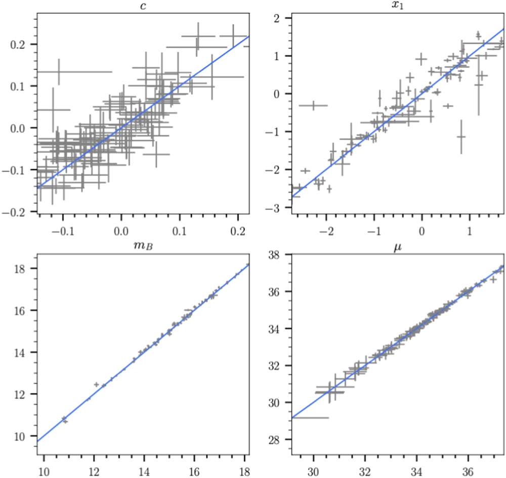
We show a comparison of the light-curve parameters of all of the duplicates in Figure 5. We see great agreement for the different fit parameters, and note the small amount of outliers are due to sparse light-curve quality that barely passes the fit (e.g., 2006ot, the largest outlier in x1 space). The significance of outliers in fit-parameter space is reduced in μ space due to covariance between light-curve parameters. For the recovered μ values, we find a standard deviation of the differences in the pairs of 0.102 mag. Following a similar bootstrapping procedure as above, and only using low-z SNe, we calculate a typical dispersion for 151 pairs of random SNe (correcting for redshift differences) to have 0.218 mag with 0.011 uncertainty. Therefore, the distances of the same SN measured by two separate surveys agree by > 10σ better than two random SNe. This insight is again important for creating the systematic covariance matrix in B22a that the intrinsic scatter of an SN Ia should be shared for measurements of the same SN by different surveys; from Equation (2),  , where the ith and jth light curves are of the same SN from different samples, and σint is the intrinsic scatter of the sample.

Figure 5. A comparison of the fit parameters of duplicate SNe. Here we compare pairs for SALT2 parameters c, x1, mB , and μ. The strong level of agreement is given in the text, and any noticeable outliers are due to sparse light-curve quality.
Download figure:
Standard image High-resolution imageIn Table 4, we present a comparison of the distance modulus of the SN duplicates between surveys. We do not find any deviations from the mean beyond 2σ. The largest deviation is from LOSS1 (Ganeshalingam et al. 2010) at 2.0σ. B22b show the mean distance-modulus residuals for each subsample for all surveys and do not find any magnitude deviations greater than 0.05 mag with the exception of CfA1. Our results here generally support the agreement found by B22b.
Furthermore, in Table 5, we give the fraction of the sample each survey contributes to the second and third rungs of the distance ladder described in R22, where the third rung has a limit of z < 0.15, and those in the second rung are determined SNe found in nearby galaxies with associated Cepheid measurements. (We note that the baseline determination of H0 further limits the third rung sample to z > 0.0233 and to late-type hosts.) Assuming (gray) survey errors, an estimate of the error in H0 from survey miscalibration results from the difference in these fractions multiplied by the mean residual of each survey from the full compilation. We give the fractional difference between these two rungs by sample and the survey residual calculated by B22b (see Figure 6) in Table 5. If one multiplies the fractional difference between rungs by the Hubble residual offsets, this describes the sensitivity of H0 (in magnitudes, not km s−1 Mpc−1) to possible discrepancies of sample offsets. We find that the largest fractional difference is due to Foundation at ∼23%, and the majority of the fractional differences are between 2% and 15%. After multiplying these differences by the Hubble residual offsets, we find the products are all below 4 mmag. This would imply a sensitivity in H0 on the level of 0.2%. This also illustrates the benefit of using a similar mix of surveys for both samples. Because we cannot avoid using a mix of surveys for the second rung (these are objects are rare), the use of a single sample for the third rung would propagate an error in H0 at the level of ∼1% as shown in Brownsberger et al.(2021).
Table 5. Fraction of SNe in the Second and Third Rungs of Distance Ladder
| SURVEY | Frac. HF (rung 3) | Frac. CAL (rung 2) | Δ (3-2) | Δμ | Δμ × Δ (3-2) (mag) |
|---|---|---|---|---|---|
| SDSS | 0.112 | 0.000 | −0.112 | 0.009 | −0.0010 |
| PS1 | 0.054 | 0.000 | −0.054 | 0.036 | −0.0019 |
| DES | 0.010 | 0.000 | −0.010 | −0.015 | 0.0001 |
| CSP | 0.083 | 0.129 | 0.046 | 0.034 | 0.0015 |
| CfA1 | 0.018 | 0.048 | 0.030 | −0.104 | −0.0031 |
| CfA2 | 0.026 | 0.048 | 0.021 | −0.023 | −0.0005 |
| CfA3 | 0.089 | 0.077 | −0.012 | −0.001 | 0.0000 |
| CfA4 | 0.054 | 0.016 | −0.038 | 0.033 | −0.0012 |
| Foundation | 0.279 | 0.052 | −0.227 | 0.008 | −0.0017 |
| CNIa0.02 | 0.018 | 0.040 | 0.022 | 0.027 | 0.0006 |
| LOWZ | 0.056 | 0.187 | 0.131 | −0.020 | −0.0002 |
| LOSS | 0.147 | 0.244 | 0.097 | 0.012 | 0.0012 |
| SOUSA | 0.057 | 0.161 | 0.105 | 0.005 | 0.0005 |
Notes. The relative fractions of SN samples by survey (accounting for duplicates) for the third rung of distance ladder (z < 0.15) SN sample, the second rung of distance-ladder Cepheid-hosted SN sample in R21, the difference between the two, the mean offset by survey given in B22b in Figure 6, and the product of the survey offset with the fractional difference. The product indicates the size of the sensitivity of H0 (in mag, not km s−1 Mpc−1—divided by ∼2 for percent units in H0) to survey miscalibration or other issues. See Brownsberger et al. (2021) for more information about this sensitivity.
Download table as: ASCIITypeset image
4. Discussion and Conclusions
In this paper, we presented the new "Pantheon+" sample that is used in a series of analyses for cosmological parameter measurements. The challenge of a compilation analysis like this one is documentation, and unlike previous analyses, we attempt here to document key properties about the samples (photometric system, data location, references) to improve reproducibility in the future.
The Pantheon+ analysis improves on the Pantheon analysis in nearly every facet. Not only do we increase the sample size, but we do a comprehensive review of the redshifts (C22) and peculiar velocities (Peterson et al. 2022), a new calibration and model retraining for the sample (B22b), and new cosmological analyses by R22 and B22a. We detail data that have been added to the previous Pantheon compilation, as well as changes to the data that were previously used. As these samples date back 40 yr, we have made a significant effort to check assumptions about how data have been passed from analysis to analysis, rather than assuming previous analyses have understood each facet correctly.
The size of a sample like this will soon be surpassed by other samples from newer and upcoming surveys like the Zwicky Transient Facility (Dhawan et al. 2021), the Young Supernova Experiment (Jones et al. 2021), the DES (Smith et al. 2020), the Legacy Survey of Space and Time (LSST; Ivezić et al. 2019), and the Nancy Grace Roman Space Telescope (Hounsell et al. 2018). These surveys may find a similar number of SNe to this compilation in only a matter of days. However, the usefulness of the Pantheon+ sample, particularly at low redshift, is unlikely to be surpassed for some time owing to its utility for constraining the Hubble constant. For this measurement, we are statistically limited by the number of SNe in nearby galaxies in which Cepheids can be found, which is typically one SN discovered per year (R22).
Two of the findings from this paper will be used to create the systematic covariance matrix of B22a. The first is that we find excellent agreement when different surveys measure the same SNe, and the second is that we find relatively poor agreement when surveys measure distances of two SNe in the same galaxy. The latter of these findings will be best tested with LSST, which can find over 800 siblings (The LSST Dark Energy Science Collaboration et al. 2018; Scolnic et al. 2020). Finally, we show that because of our effort to include samples that cover the second and third rungs of the distance ladder, the accuracy of the H0 measurement will not be limited by possible discrepancies in measurements of the SN distances by sample.
D.S. is supported by Department of Energy grant DE-SC0010007, David and Lucile Packard Foundation, and the John Templeton Foundation grant 62314. This manuscript is based upon work supported by the National Aeronautics and Space Administration (NASA) under contracts NNG16PJ34C and NNG17PX03C issued through the WFIRST Science Investigation Teams Program. D.S. and R.J.F. are supported in part by NASA grant 14-WPS14-0048. T.M.D. and A.C. are supported by an Australian Research Council Laureate Fellowship, FL180100168. D.O.J. is supported by NASA through Hubble Fellowship grant HF2-51462.001 awarded by the Space Telescope Science Institute (STScI), which is operated by the Association of Universities for Research in Astronomy, Inc., for NASA, under contract NAS5-26555. P.J.B.'s work is supported by NASA ADAP grant 80NSSC20K0456: "SOUSA's Sequel: Improving Standard Candles by Improving UV Calibration." The Pan-STARRS1 Surveys (PS1) and the PS1 public science archive have been made possible through contributions by the Institute for Astronomy, the University of Hawaii, the Pan-STARRS Project Office, the Max-Planck Society and its participating institutes, the Max Planck Institute for Astronomy, Heidelberg and the Max Planck Institute for Extraterrestrial Physics, Garching, The Johns Hopkins University, Durham University, the University of Edinburgh, the Queen's University Belfast, the Harvard-Smithsonian Center for Astrophysics, the Las Cumbres Observatory Global Telescope Network Incorporated, the National Central University of Taiwan, STScI, NASA under grant NNX08AR22G issued through the Planetary Science Division of the NASA Science Mission Directorate, National Science Foundation (NSF) grant AST-1238877, the University of Maryland, Eotvos Lorand University (ELTE), the Los Alamos National Laboratory, and the Gordon and Betty Moore Foundation. D.B. acknowledges support for this work provided by NASA through the NASA Hubble Fellowship grant HST-HF2-51430.001 awarded by STScI. A.V.F.'s group at U.C. Berkeley acknowledges generous support from Marc J. Staley (whose fellowship partly funded B.E.S. while contributing to the work presented herein as a graduate student), the TABASGO Foundation, the Christopher R. Redlich fund, the Miller Institute for Basic Research in Science (in which A.V.F. is a Miller Senior Fellow), and many individual donors. The UCSC team is supported in part by NSF grants AST-1518052 and AST-1815935, the Gordon & Betty Moore Foundation, the Heising-Simons Foundation, and from fellowships from the Alfred P. Sloan Foundation and the David and Lucile Packard Foundation to R.J.F. D.A.C. acknowledges support from the National Science Foundation Graduate Research Fellowship under grant DGE1339067. M.R.S. is supported by the National Science Foundation Graduate Research Fellowship Program under grant No. 1842400.
KAIT (for LOSS) and its ongoing operation were made possible by donations from Sun Microsystems, Inc., the Hewlett-Packard Company, AutoScope Corporation, Lick Observatory, the NSF, the University of California, the Sylvia & Jim Katzman Foundation, and the TABASGO Foundation. Research at Lick Observatory is partially supported by a generous gift from Google.
Simulations, light-curve fitting, BBC, and cosmology pipeline are managed by PIPPIN (Hinton & Brout 2020). Contours and parameter constraints are generated using the ChainConsumer package (Hinton 2016). Plots are generated with Matplotlib (Hunter 2007). We used astropy (Price-Whelan et al. 2018), SciPy (Virtanen et al. 2020), and NumPy (Oliphant 2006).
D.B. thanks his spouse Isabella and their future daughter for their support as the due date is rapidly approaching!
Appendix A: Data-release Structure
The data release will be found at https://pantheonplussh0es.github.io/. It will also be found in the public version of SNANA in the "Pantheon+" directory. The SNANA full data download is available via Kessler & Brout (2020), and the SNANA source directory is https://github.com/RickKessler/SNANA.
The structure of the Pantheon+ directory contains 18 subdirectories, with folder names synced to the data samples listed in Table 1. In each folder, there is a .README file with documentation of the source of the data files, and an .LIST file that lists the SNe Ia fitted as part of this analysis. In each subdirectory, there are .txt files or .FITS describing the SN light curves along with meta-information. If there are .txt files, the meta-information is at the top of the file, whereas if there is an .FITS file, the meta-information is in the HEAD.FITS file while the light-curve data are in the PHOT.FITS file. For a single .txt file for one light curve, we show an example screenshot in Figure 6.

Figure 6. Display of what an SNANA light-curve file looks like for SN 2021pit. The full file is included at https://pantheonplussh0es.github.io/.
Download figure:
Standard image High-resolution imageThe meta-information includes the following:
- 1.SN name
- 2.SN position: R.A., decl. in degrees and host position.
- 3.SN Milky Way extinction (though this is overridden in fitting to ensure consistency with Schlafly & Finkbeiner 2011).
- 4.The heliocentric redshift, CMB-frame redshift, and peculiar velocity VPEC.
The light-curve data has columns for date (MJD), filter (FLT), flux (FLUXCAL), flux uncertainty (FLUXCALERR), magnitude (MAG), and magnitude uncertainty (MAGERR). The common zero-point for all flux measurements is 27.5 mag.
We also include several global files for various properties. These include the following:
- 1.List of heliocentric, CMB, and peculiar velocities as derived by C22.
- 2.List of all host-galaxy properties determined for this analysis. These include mass for all SNe, and SFR and morphology for SNe with z < 0.15.
Finally, we include a combined file of all of the fitted parameters for each SN, before and after light-curve cuts are applied. This is in the format of an .FITRES file and has all of the meta-information listed above along with the fitted SALT2 parameters. We show a screenshot of the release in Figure 7. Here, we give brief descriptions of each column. CID—name of SN. CIDint—counter of SNe in the sample. IDSURVEY—ID of the survey. TYPE—whether SN Ia or not—all SNe in this sample are SNe Ia. FIELD—if observed in a particular field. CUTFLAG_SNANA—any bits in light-curve fit flagged. ERRFLAG_FIT—flag in fit. zHEL—heliocentric redshift. zHELERR—heliocentric redshift error. zCMB—CMB redshift. zCMBERR—CMB redshift error. zHD—Hubble Diagram redshift. zHDERR—Hubble Diagram redshift error. VPEC—peculiar velocity. VPECERR—peculiar-velocity error. MWEBV—MW extinction. HOST_LOGMASS—mass of host. HOST_LOGMASS_ERR—error in mass of host. HOST_sSFR—sSFR of host. HOST_sSFR_ERR—error in sSFR of host. PKMJDINI—initial guess for PKMJD. SNRMAX1—First highest signal-to-noise ratio (S/N) of light curve. SNRMAX2—Second highest S/N of light curve. SNRMAX3—Third highest S/N of light curve. PKMJD—Fitted PKMJD. PKMJDERR—Fitted PKMJD error. x1—Fitted x1. x1ERR—Fitted x1 error. c—Fitted c. cERR—Fitted c error. mB—Fitted mB . mBERR—Fitted mB error. x0—Fitted x0. x0ERR—Fitted x0 error. COV_x1_c—covariance between x1 and c. COV_x1_x0—covariance between x1 and x0. COV_c_x0—covariance between c and x0. NDOF—number of degrees of freedom (epochs) in light-curve fit. FITCHI2—χ2 of light-curve fit. FITPROB—fit probability. RA—RA of SN (deg). DEC—DEC of SN (deg). HOST_RA—RA of host (deg). HOST_DEC—DEC of host (deg). HOST_ANGSEP—Separation between SN and host (deg). TGAPMAX—largest gap (in days) between observations. TrestMIN—minimum epoch with SN observation (day). TrestMAX—maximum epoch with SN observation (day). ELU—morphological classification.

Figure 7. Display of what an .FITRES file looks like that has all of the information from the light-curve fit, as well as ancillary information. A value of −9 is given where information is unavailable. The full file will be included at pantheonplussh0es.github.io.
Download figure:
Standard image High-resolution image
Appendix B: SN Data Information
In Table 6 and 7, we present the summary information for the low-z and high-z samples respectively. We summarize the paper in which the sample is published, the location of the data, and the photometric system of the data.
Table 6. Low-redshift SN Photometry Data Releases and Access
| Question | Answer |
|---|---|
| CfA1 | |
| Where are the SN data published? | Riess et al. (1999) |
| Where is the site for the SN data? | https://www.cfa.harvard.edu/supernova/SNarchive.html |
| What system is the SN in? | Standard |
| CfA2 | |
| Where are the SN data published? | Jha et al. (2006) |
| Where is the site for the SN data? | https://iopscience.iop.org/article/10.1086/497989/fulltext/204512.tables.html |
| What system is the SN in? | Standard |
| CfA3-Kepler-cam | |
| Where are the SN data published? | Hicken et al. (2009) |
| Where is the site for the SN data? | https://www.cfa.harvard.edu/supernova/CfA3/ |
| What system is the SN in? | Standard and Natural |
| CfA3-4Shooter | |
| Where are the SN data published? | Hicken et al. (2009) |
| Where is the site for the SN data? | https://www.cfa.harvard.edu/supernova/CfA3/ |
| What system is the SN in? | Standard and Natural |
| CfA4p1 | |
| Where are the SN data published? | Hicken et al. (2012) |
| Where is the site for the SN data? | https://www.cfa.harvard.edu/supernova/CfA4/ |
| What system is the SN in? | Standard and Natural |
| CfA4p2 | |
| Where are the SN data published? | Hicken et al. (2012) |
| Where is the site for the SN data? | https://www.cfa.harvard.edu/supernova/CfA4/ |
| What system is the SN in? | Standard and Natural |
| CNIa0.02 | |
| Where are the SN data published? | Chen et al. (2020) |
| Where is the site for the SN data? | Private communication |
| What system is the SN in? | Natural |
| CSP DR3 | |
| Where are the SN data published? | Krisciunas et al. (2017b) |
| Where is the site for the SN data? | https://csp.obs.carnegiescience.edu/data/CSP_Photometry_DR3.tgz/view |
| What system is the SN in? | Natural |
| LOSS1 | |
| Where are the SN data published? | Ganeshalingam et al. (2010) |
| Where is the site for the SN data? | http://heracles.astro.berkeley.edu/sndb/info |
| What system is the SN in? | Natural |
| LOSS2 | |
| Where are the SN data published? | Stahl et al. (2019) |
| Where is the site for the SN data? | http://heracles.astro.berkeley.edu/sndb/info |
| What system is the SN in? | Natural |
| SOUSA | |
| Where are the SN data published? | Brown et al. (2014) |
| Where is the site for the SN data? | https://pbrown801.github.io/SOUSA/ |
| What system is the SN in? | VEGA |
| Foundation | |
| Where are the SN data published? | Foley et al. (2018) |
| Where is the site for the SN data? | https://github.com/djones1040/Foundation_DR1 |
| What system is the SN in? | AB |
Note. In addition to the surveys listed here, there are individual releases of SN photometry as listed for LOWZ in Table 1.
Download table as: ASCIITypeset image
Table 7. High-redshift SN Photometry Data Releases and Access
| Question | Answer |
|---|---|
| PS1 | |
| Where are the SN data published? | Scolnic et al. (2018) |
| Where is the site for the SN data? | https://archive.stsci.edu/hlsps/ps1cosmo/jones/lightcurves/ |
| What system is the SN in? | AB |
| SDSS | |
| Where are the SN data published? | Sako et al. (2018) |
| Where is the site for the SN data? | http://sdssdp62.fnal.gov/sdsssn/DataRelease/index.html |
| What system is the SN in? | AB |
| SNLS | |
| Where are the SN data published? | Betoule et al. (2014) |
| Where is the site for the SN data? | https://supernovae.in2p3.fr/sdss_snls_jla/ReadMe.html/ |
| What system is the SN in? | AB |
| DES | |
| Where are the SN data published? | Brout et al. (2019b) |
| Where is the site for the SN data? | https://des.ncsa.illinois.edu/releases/sn/ |
| What system is the SN in? | AB |
Note. In addition to the surveys listed here, there are HST survey light curves as per the HDFN, SCP, CANDELS+CLASH, and GOODS+PANS references in Table 1.
Download table as: ASCIITypeset image
Footnotes
- 21
Light curves from SOUSA can be found at https://pbrown801.github.io/SOUSA/.