


Abstract
In this work, we derive magnetic toroids from surface magnetograms by employing a novel optimization method, based on the trust region reflective algorithm. The toroids obtained in this way are combinations of Fourier modes (amplitudes and phases) with low longitudinal wavenumbers. The optimization also estimates the latitudinal width of the toroids. We validate the method using synthetic data, generated as random numbers along a specified toroid. We compute the shapes and latitudinal widths of the toroids via magnetograms, generally requiring several m's to minimize residuals. A threshold field strength is chosen to include all active regions in the magnetograms for toroid derivation, while avoiding non-contributing weaker fields. Higher thresholds yield narrower toroids, with an m = 1 dominant pattern. We determine the spatiotemporal evolution of toroids by optimally weighting the amplitudes and phases of each Fourier mode for a sequence of five Carrington Rotations (CRs) to achieve the best amplitude and phases for the middle CR in the sequence. Taking more than five causes "smearing" or degradation of the toroid structure. While this method applies no matter the depth at which the toroids actually reside inside the Sun, by comparing their global shape and width with analogous patterns derived from magnetohydrodynamic (MHD) tachocline shallow water model simulations, we infer that their origin is at/near the convection zone base. By analyzing the "Halloween" storms as an example, we describe features of toroids that may have caused the series of space weather events in 2003 October–November. Calculations of toroids for several sunspot cycles will enable us to find similarities/differences in toroids for different major space weather events.
Export citation and abstract BibTeX RIS
1. Introduction
There is ample evidence from various observations that active regions manifest at the solar surface in a globally organized pattern, both in time and space. Magnetic fields in active regions virtually always obey Hale's polarity law, i.e., that leader and follower spots have opposite polarities in northern and southern hemispheres. The zone of latitudes where spots are seen migrates toward the Equator in each sunspot cycle, tracing out the well-known butterfly diagram. There is also a short-term periodicity of 6–18 months within a solar cycle. This Rieger-type periodicity (Rieger et al. 1984; Oliver et al. 1998; Zaqarashvili1 et al. 2010), which produces the "seasons" of solar activity, manifests in the progress of a solar cycle, in the form an enhanced burst of activity, followed by a relatively quiet period (McIntosh et al. 2015; Dikpati et al. 2017). There is also a global organization in the spatial pattern of the emerged active regions—often referred to as "active longitudes," which have been observed for more than a century (Maunder 1905). The persistence of active longitudes can range from several Carrington Rotations (de Toma et al. 2000) to several solar cycles (Benevolenskaya et al. 1999; Kostyuchenko & Benevolenskaya 2015; Mandal et al. 2017). While there may be some departures in the spatiotemporal organization of emerging active regions, their origin is somewhere below the photosphere, rather than merely the result of turbulent processes on the surface. In order to understand the physical origin of the spatiotemporal evolutionary patterns of active regions at the surface, it is necessary to infer global properties, such as their shape and its time variation, from surface magnetogram observations.
Extensive studies of the magnetohydrodynamics of tachocline latitudinal differential rotation, with coexisting spot-producing magnetic fields, have been conducted over the past two decades, since Gilman & Fox (1997) revealed certain global features in the patterns of toroidal field and tachocline shear flow. These features include instabilities in differential rotation and toroidal fields, leading to global magnetic patterns at the tachocline with low longitudinal wavenumbers (m = 1 through 7 or so), which have similar scales and lifetimes to synoptic magnetic features seen on the solar surface. The nonlinear interaction of MHD Rossby waves with toroidal magnetic fields and differential rotations demonstrates that the resulting nonlinear, quasiperiodic oscillation in the energies of magnetic fields, differential rotation, and Rossby waves might plausibly be the origin of solar (short-term) "seasonal" variability, i.e., variations of activity on timescales of 6–18 months. These features cause us to identify the tachocline as the most likely origin of global organization in the surface magnetism of the Sun. The global models employed to obtain these results are 2D and 3D thin-shell shallow water-type models. Cally and colleagues (Cally 2001; Cally et al. 2003) first discovered the clamshell opening up of a broad toroidal magnetic field, and the tipping of a banded toroidal field, during the nonlinear evolution of 2D global MHD of the tachocline.
Extending these nonlinear 2D MHD tachocline instabilities to include a 3D thin-shell shallow water-type model's tipping of toroidal bands has also been reconfirmed. Shallow water models are applied to the tachocline because the stratification is at least slightly subadiabatic; as such, variations in flows and magnetic fields are much smaller in radial than in horizontal directions. Only latitudinal differential rotation is included in a single-layer version of this class of models, which has one layer whose top, interfacing with the convection zone, is allowed to deform. Therefore, in principle, similar models can be applied to a thin layer (or may even permit a thicker domain) in the lower half of the convection zone, if the stratification is subadiabatic. Such a structure has been suggested, based on certain nonlinear turbulent convection simulations (Käpylä et al. 2017).
Norton & Gilman (2005) searched for evidence of the tipping instability, using the Kitt Peak National Observatory (KPNO) magnetogram data for Carrington Rotations 1645–1991, as well as Michelson Doppler imager (MDI) continuum intensity sunspot data, covering about thirty years during cycles 21–23. Since the longitudinal wavenumber m = 1 mathematically represents a tipped ring, Norton & Gilman (2005) computed the amount of tip as function of cycle phase by fitting a sine function, the amplitude of which gives the tip. Their estimated tip was found to match the features obtained from the magnetorotational instabilities of a 2D toroidal band. On the basis of the MDI data, and a model calculation with synthetic input, they determined that the best fit of the data was for a toroidal bandwidth of 10° for high sunspot latitudes early in a cycle. For low latitudes late in a cycle, the best fit was for a broader band of 20°, with tip declining to zero.
In an independent calculation, P. Ambroz (2021, private communication) looked for evidence of tipping in a magnetic toroid by fitting an m = 1 sinusoid to sunspot location data from KPNO. He found similar tipping as a function of cycle phase, and estimated the bandwidth from the spread in the fitting. Noting that pure tipping is a feature of a strong toroidal band (with ∼100 kGauss peak field strength), and hence behaves like a "steel" ring, we can associate this tipping with a strong solar cycle, and/or active regions, appearing primarily near the band center. In relatively weaker cycles, and from time to time in the presence of active regions from weaker peripheral regions of the magnetic band, higher longitudinal wavenumbers can dominate the dynamics of the band. This weakening may also be due to the spread in latitudinal width of the band, which can widen due to certain forms of dynamical evolution, while conserving the total flux within it. Weaker bands (with a peak field strength of <35 kGauss) deform more than they tip, implying the existence of m > 1 modes as well as the m = 1 mode (see, e.g., Cally et al. 2003).
Further developments of nonlinear 3D thin-shell and shallow water-type models (Dikpati 2012; Dikpati et al. 2018) provide essential new features, due to the presence of potential energy, along with the kinetic and magnetic energies of the system. On the one hand, the additional properties obtained from 3D models complicate the evolution of tipping/deformation patterns due to nonlinear exchange among energy reservoirs (Tachocline Nonlinear Oscillations); on the other hand, they provide latitude–longitude locations of flux eruptions from the tachocline top surface bulges, containing spot-producing toroidal fields (Dikpati & Gilman 2005; Dikpati et al. 2017). Recently, Dikpati & McIntosh (2020) demonstrated that model outputs of toroidal fields in tachocline top surface bulges evolve in accordance with the evolution of emerging active regions' locations, as observed in the magnetograms.
Based on the above discussion of the theoretical framework of the tipping/deformation of a toroidal magnetic band at the base of the convection zone, as well as efforts to reproduce band tipping based on surface observations, we favor the idea that dynamo-generated spot-producing magnetic toroids reside at the base of the convection zone and/or in the overshoot tachocline, and logically conjecture that the nonlinear magnetohydrodynamics of these toroids are the origins of the global patterns manifesting in surface bipolar active regions. Therefore, in this work we explore comparisons of our observational analysis to theoretical models of the magnetohydrodynamics of toroids to emphasize whether models of the global MHD of the tachocline can plausibly be the physical origin of the systematic component of the spatiotemporal pattern of active regions. However, we recognize that it has been argued that spot-producing toroids are contained within the bulk of the convection zone, since some global convectively driven MHD dynamo models (Nelson et al. 2013b) produce "wreaths" of toroidal fields in this domain. It has also been argued that the spot-producing magnetic fields could instead be generated in the near-surface shear layer, i.e., just the outer few percent of the solar interior (Brandenburg 2005). However, these models have not yet compared the spatiotemporal global evolution of model-generated shapes and widths of the toroids with observations. The observational analyses we present in this paper will provide clues as to the shape and time evolution of toroids, at whatever depth they reside in the Sun; as such, these properties should be of interest, no matter at which depth they are thought to reside, or by what physical mechanism they are produced.
To deduce more detailed properties of surface toroids, and relate them to the magnetohydrodynamics of bottom toroidal fields, or higher-level toroids produced by others, using convective, or near-surface shear layer models, it is necessary to develop a generalized methodology and a numerical scheme, building on previous efforts (Norton & Gilman 2005) (also Ambroz 2021, private communication) relating to m = 1 sinusoid fitting.
The main aim of this paper is to analyze magnetograms so as to extract the global pattern in active regions' emergence locations, thereby deriving how various longitudinal wavenumbers' m ≥ 0 modes contribute to form the global pattern in magnetic toroids manifesting at the solar surface, the latitude-centroid of these toroids, and their latitudinal widths. We will compare the observed patterns with model-generated global patterns at the tachocline. Many intriguing questions arise: can we extract the dominant Fourier modes present in the active regions' global pattern? How do these modes evolve over several Carrington Rotations (CRs)? Can we infer the latitudinal width of the bottom magnetic band, from which the surface active regions likely originate, and how does the bandwidth of the magnetic band vary with time? Given the existence of north–south asymmetry in the patterns of active regions at the surface, can we determine how the symmetry/asymmetry between the two bands in the two hemispheres evolves and flips with time? What other properties can we infer? If the dominant Fourier mode turns out to have the longitudinal wavenumber m = 1, the mode can be represented by a pure sinusoid, whose amplitude will give the tip angle with respect to the m = 0 mode, which would denote the mean latitude. Therefore, for the m = 1 mode, the maximum and minimum latitudes, with respect to the mean latitude (m = 0), are 180° apart in longitude, and thus the amplitude of the m = 1 mode is the measure of the tip angle. Can we estimate the tip angle of the spot-producing toroidal band with respect to the polar axis using our scheme? While we cannot fully answer all of the above questions based on the few sample cases used here, this work attempts to address most of them qualitatively, and to explore a plausible physics behind them. Subsequent papers will dig deeper, examining larger numbers of observational analyses and model simulations, using the methodology we introduce here.
2. Analysis from Magnetograms
Our starting point is the Solar and Heliospheric Observatory (SOHO)/MDI magnetograms. We download the available magnetogram data in FITS format. The line-of-sight corrected radial magnetic field data is laid out in 1080 × 3600 synoptic gridpoints in sine(latitude) × longitude. We note that magnetic field synoptic maps are constructed in Carrington coordinates by merging together solar observations derived from central meridian data from full-disk magnetograms taken over full Carrington periods.
We create a set of synoptic maps for several Carrington Rotations. Considering a plausible scenario whereby the global organizations of the erupted bipolar active regions at the surface are being governed by the dynamics of the dynamo-generated spot-producing toroidal fields in deep layers at/near the base of the convection zone, we can estimate the position, latitudinal width, and band center of the underlying pair of magnetic toroids, from which the strong fields erupt to the surface in the form of bipolar active regions. Our goal is to extract a map or layout of these toroids with respect to both latitude and longitude. To do this, we retain the bipolar regions by selecting fields in their heliographic latitude and longitude positions above a threshold amplitude, and finding the best Fourier mode(s) fitted to these points. Thus Fourier modal curve(s) are obtained over all longitudes of the Sun in each hemisphere. A modal pattern of longitudinal wavenumber 1 gives a measure of the tilt or slope of the magnetic toroid with respect to the central axis (polar axis).
The data near polar regions are uncertain, so they are excluded. We use data bounded by ±65° latitudes. This choice helps us extract the toroids without loss of generality, because all active regions appear within that latitude range. Furthermore, we know that north/south asymmetry exists in terms of solar cycle properties. Therefore, we derive the patterns and bandwidth of the toroids in each hemisphere by optimizing the spatial locations of active regions separately in the north and south.
2.1. Formulation of Numerical Scheme
In order to derive the global patterns manifesting in the surface's active regions, we utilize the following information gathered from the observed synoptic magnetograms: (i) Along with the bipolar active regions containing strong magnetic field, there is also a coexistent weak background magnetic field throughout the entire magnetogram. However, since the magnetic fields in active regions is stronger than their surroundings, they can be identified using a reasonably high threshold value, below which the field data is excluded from the optimization process. (ii) In each hemisphere, the active regions manifest in a relatively narrow belt in latitude, and one or more longitudes; (iii) the latitude–longitude locations of active regions vary only very slowly with time from one CR to the next.
Along with the above considerations, we also take into account that the synoptic maps represent all longitudes of the Sun, and hence the longitudinal boundaries are periodic. As such, the most general form we can consider to represent the latitude center of the global pattern (Pc ) in each hemisphere is as follows:


Here, Pc is a function of longitude, (ϕ), and a slowly varying function of time (t); q0 is the mean latitudinal location of the pattern (i.e., the m = 0 Fourier mode), qm is the amplitude of the Fourier mode with longitudinal wavenumber m, and ζm is the phase of the mth Fourier mode. Note that t, the time in units of CR, appears in Equations (2)–(3) to facilitate information propagation from neighboring CR periods, which becomes significant during a CR, when active regions are relatively sparse. In Equations (2) and (3), si,m and wi,m , respectively, represent the time-varying parts of amplitudes, and phases of different m modes. We will discuss this temporal effect below, while reconstructing the global pattern using multiple CRs. For the time being, we are setting t = 0 in order to study the synoptic maps of a single CR.
We note that our formulation includes a significant number of parameters, so we can safely avoid "underperforming," which may cause difficulty in extracting temporal evolution. On the other hand, we have to be cautious about "overperforming," which may also lead to poor generalization. Therefore, we need a method that allows us to specify constraints and bounds in parameters. The "Trust Region Reflective" (TRR) algorithm (Branch et al. 1999) is such a scheme, and is employed in our problem, following the implementation methodology given in the tutorial of SciPy, a piece of open source software for science, mathematics, and engineering (see, e.g., "scipy.optimize.least_squares").
Even though the TRR scheme has been used extensively in many large-scale optimization problems in physics, we are not aware of its use in magnetogram analysis. As such, a very brief description of the TRR scheme may be helpful to readers. In our case, we need to optimize our objective function over many parameters, involving many thousands of data points with constraints in the parameter space. If we approach this problem naively this might prove infeasible, as well as computationally expensive, since it would essentially require the evaluation of the function at every point in the parameter space. This would lead to considering reasonably spaced grids of parameters of dimensions equal to the number of parameters. The TRR method is a robust and efficient algorithm that heuristically approximates (or trusts) the objective function via a model function, which is a relatively cheaper means to evaluate and predict the minimum point within the region of validity of this model function. The region is determined and validated dynamically as it progresses iteratively. The validation requires actual evaluation of the objective function. If the validity fails, it then contracts the region iteratively until it succeeds. On the other hand, if it succeeds, it tries to be more aggressive in expanding the region in the next iteration. In this way, within a reasonable number of evaluations of the actual objective function (in practice several thousands), it arrives at the minimum point in the parameter space (Conn et al. 2000).
As can happen with all non-annealed optimization problems, a particular algorithm may get stuck in a local minimum. We therefore verify our results by (i) choosing many initial guesses of parameters, and (ii) employing another algorithm, i.e., the Levenberg–Marquardt algorithm (More 1977). We solve both the codes (based on both the TRR and Levenberg–Marquardt algorithms) in Python and MATLAB for code validation.
Moreover, we need to set a minimum magnetic field amplitude, so that only fields above this threshold contribute to determining the pattern. Too low a threshold would result in including magnetic fields outside the active regions, which may not be connected to a toroid at the base of the convection zone; too high a threshold leads to missing some or all active regions. We will present results showing how the choice of threshold field influences the features of the Fourier-mode patterns.
The optimal solution for the global pattern, Pc (ϕ), is obtained at the minimum of least-square surface in the dimension of all parameters involved. As stated above, q0 gives the mean latitude (the central latitude), which is essentially the m = 0 component of the magnetic toroid as function of longitude (ϕ). At the minimum point on the least-square surface, we also obtain the covariant matrix. The square root of the diagonal elements of this matrix provides a measure of uncertainties in respective parameters. The uncertainty in the mean (q0) gives us the estimate of the latitudinal width for Pc , implying that the active regions considered for deriving the global magnetic toroid fall within this latitudinal extent on both sides of the mean or central band latitude.
3. Results
3.1. Magnetic Toroids Derived from Synthetic Data
Our first step is to validate the code using "synthetic" data. In order to do this, we construct a "synthetic" global pattern by setting up a mathematical prescription as:

in which the mean latitude center is  the amplitudes of three modes with longitudinal wavenumbers m = 1, 2, 3 are
  ,
,  ,
,  and the phases with which these modes combine to form the global pattern are
  ,
,  and
and  in degrees.
From this pattern, we can prescribe the eruption of active regions, using random locations around the central latitude within an approximate 6° spread. By implementing our optimization scheme, based on the trust region reflective algorithm as described above, we extract the optimized set of  ,
,  and
and  for various m modes. Figures 1(a) and (b) display the derived patterns for two different realizations of erupted active regions, obtained using two sets of random numbers for 15 locations.
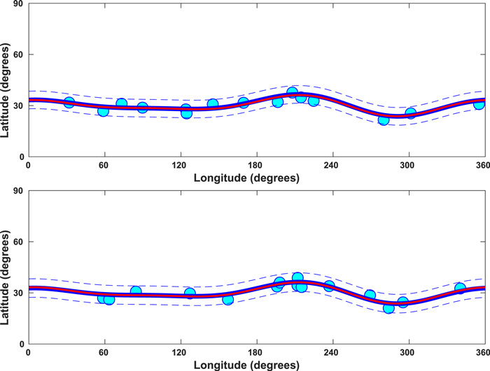
Figure 1. Magnetic toroid patterns derived from synthetic data; the two cases are for two different realizations of erupted active regions.
Download figure:
Standard image High-resolution imageThe cyan filled circles in both panels of Figure 1 represent the latitude–longitude locations of erupted active regions, the blue curve is the pattern obtained employing our optimization scheme, and the superimposed red curve is the true pattern given by expression (4).
The optimized values for the two cases in Figure 1, along with the original values set in expression (4), are given in Table 1 for comparison. We can see that these values validate our scheme reasonably well. Various tests indicate improvements with more data due to improved statistics in the optimization.
Table 1. Comparison of True Values with those Derived from Optimization

|

|

|

|

|

|

| |
|---|---|---|---|---|---|---|---|
| True case | 30.00 | 1.00 | 4.00 | 2.00 | −90.00 | 45.00 | 135.00 |
| Figure 1(a) case | 30.13 | 1.18 | 4.18 | 1.93 | −90.79 | 44.24 | 133.01 |
| Figure 1(b) case | 29.96 | 1.27 | 3.97 | 1.96 | −88.02 | 43.90 | 135.44 |
Download table as: ASCIITypeset image
As mentioned above, we must avoid the problem of both underperformance and overperformance in reconstructing a global pattern. This means that a global pattern needs to be prescribed using an optimal number of modes, which will be estimated by our numerical scheme in order to derive the pattern. We demonstrate a situation of underperformance by reconstructing a pattern from synthetic data. We again consider the true global pattern given by Equation (4), with same values for the q and ζ parameters. In a very similar way to that described above, we synthetically generate twenty random locations of erupted active regions around the central latitude ( ), once again within a 6° spread.
We attempt to reconstruct the pattern (Equation (4)) with only three parameters:  ,
,  , and
, and  . Figure 2 displays the results. Comparing the result with the true pattern (red curve), we can see that the reconstruction (blue curve) is poor, and the standard deviation obtained from the diagonal elements of the covariant matrix is unacceptably large, leading to unrealistic bandwidth. Therefore, underperformance may lead to inaccurate results.

Figure 2. The blue curve shows an undererperformance in deriving a "synthetic" global pattern; the cyan filled circles represent erupted active regions' locations, and the red curve is the true pattern.
Download figure:
Standard image High-resolution imageSimilarly, we demonstrate overperformance by attempting to reconstruct the true pattern given by Equation (4) using several additional parameters, i.e., considering  and
and  for m = 0 through 5. This means we are considering the combination of five Fourier modes (m = 1, 2, 3, 4, 5) and their phases, along with the mean central latitude given by
  . Note that these additional Fourier modes with longitudinal wavenumbers m = 4 and 5 are not present in the true pattern. By synthetically generating twenty random locations of erupted active regions around the central latitude (
 ) within a 6° spread, we apply our optimization scheme to reconstruct the true pattern.
We display the reconstruction in Figure 3, in which the cyan filled circles again represent the locations of erupted active regions, the blue curve is the reconstructed pattern, and the superimposed red curve is the true pattern. Figure 3 reveals that the realization of twenty random locations of active regions are well-represented by a multi-modal pattern. The amplitudes and phases of the m = 1, 2, and 3 modes are reproduced with less than 5% error, while the additional modes (m = 4, 5) contribute only insignificantly, with amplitudes of about 2% and 1.5% respectively. Features of the TRR algorithm help constrain overperformance by specifying bounds on the parameters used. Our scheme will therefore be able to deal with the overspecification of parameters.
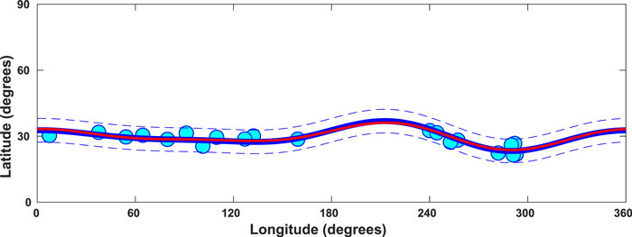
Figure 3. The blue curve denotes a reconstruction based on overperformance. It matches well with the true pattern (superimposed red curve), because the resulting amplitudes of the additional modes are insignificant. The cyan filled circles represent the locations of erupted active regions, and the bandwidth results are correct.
Download figure:
Standard image High-resolution image3.2. Properties of Magnetic Toroids Derived from an Individual Synoptic Map
Our next step is to derive the optimized set of qm and ζm for various m modes when considering a synoptic map of individual CRs (i.e., t = 0 case). Equation (4) also applies for an individual CR. As an example, we select CR 1960, which represents a time near the end of 2000 February, i.e., during the late rising phase of cycle 23. We include all active regions with a field strength above 500 Gauss per pixel. In the next subsection, we show how the derived pattern may change with the selection of cut-off field strength.
We optimize the amplitudes and phases by including modes up to m = 5, and derive the global pattern of the magnetic toroid. The TRR method estimates the centroid of the total unsigned fields of each bipolar active region, then evaluates the optimal functional form. In all optimizations, the m = 0 mode is always included, via the term  given in Equation (4). Five panels of Figure 4 display the results for successively increasing combinations of longitudinal modes, i.e., only m = 0, 1 in the top panel, m = 0, 1, and 2 in the second panel from the top, m = 0, 1, 2, and 3 in the third panel, and so on.

Figure 4. Magnetic toroid patterns derived from SOHO/MDI synoptic magnetograms for CR 1960: panels from the top to the bottom display patterns optimized for the m = 1 mode only, a combination of m = 1 and 2 modes, combinations of m = 1, 2, and 3, m = 1–4, and m = 1–5 modes, respectively. Note that the m = 0 mode is always included, via the term  given in Equation (4).
Download figure:
Standard image High-resolution imageThe five panels in Figure 4 reveal several features. Firstly, the tipping of the toroids in both hemispheres is obtained in the top panel of Figure 4. We see that the tipped toroids are more in-phase than anti-phase, but do not exist purely in either of these two phases. Secondly, examination of all five panels indicates that pure tipping is not the best optimized pattern we can derive for this case. This is due to the fact that, by setting the threshold at 500 Gauss per pixel, we permitted the inclusion of many weaker bipolar regions; MHD theory indicates that m > 1 modes dominate the dynamics of weak fields. We measure how tightly the active regions can be accommodated within a narrowest possible latitudinal width of a toroid, and find that the m = 1 pattern does not produce the smallest bandwidth. Instead, in both hemispheres, the best optimized pattern results from the combination of m = 1–4 modes (fourth panel from the top), although the maximum contribution comes from the m = 3 mode. The central latitudes remain more or less the same in both hemispheres for all five panels, but we can see that the toroid in the south has progressed forward by a few degrees more than the north toroid, implying an asymmetry in cycle phase. There is some north–south asymmetry in the bandwidth also; the toroid in the south is wider than that in the north by a few degrees.
In order to see the entire longitude range, we have presented Figure 4 in synoptic map form, with the derived magnetic toroid pattern superimposed. Figure 5 depicts what the magnetic toroid looks like in spherical geometry. In this perspective view, we see one side at a time. This example is essentially the third frame of Figure 4, in which the magnetic toroid pattern is derived considering the Fourier modes m = 0–3.
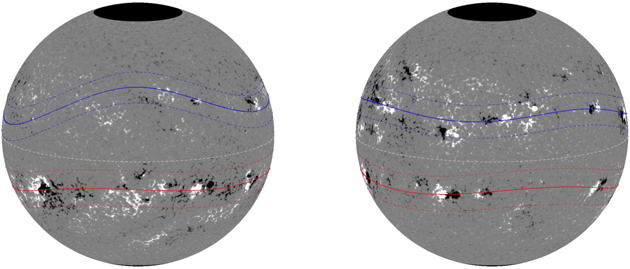
Figure 5. An example for the derived toroid pattern projected in spherical geometry; left and right panels display perspective views of front and back sides, rotated 180° in longitude with respect to each other. This case is derived for CR 1960, optimized with m = 1, 2, 3 (i.e., the third panel of Figure 4, projected onto the surface sphere. In all optimizations, the m = 0 mode is automatically included via the  term in Equation (4). The left panel shows the central part of the third panel of Figure 4 for the longitude range 70°–250°, and the right panel shows the back side of the left panel, i.e., for the longitude range from 250 to (360+70) degrees of the third panel of Figure 4.
Download figure:
Standard image High-resolution imageWe show another example of derived toroids for CR 1962 in Figure 6 based on the choice of the same threshold field of 500 Gauss. In this case, the top panel again shows the more in-phase than anti-phase tipping of the toroids in both hemispheres. This is not surprising, because the systematic component in the global patterns is a slowly varying function of time. In general, the magnetic toroids are narrower in this case than in Figure 4. Examination of all panels indicates that the best toroid can be derived for combinations of m = 0–5 modes in the north, but for m = 0–4 modes in the south. The bandwidths in both hemispheres are nearly the same, but north–south asymmetry arises in the number of modes.
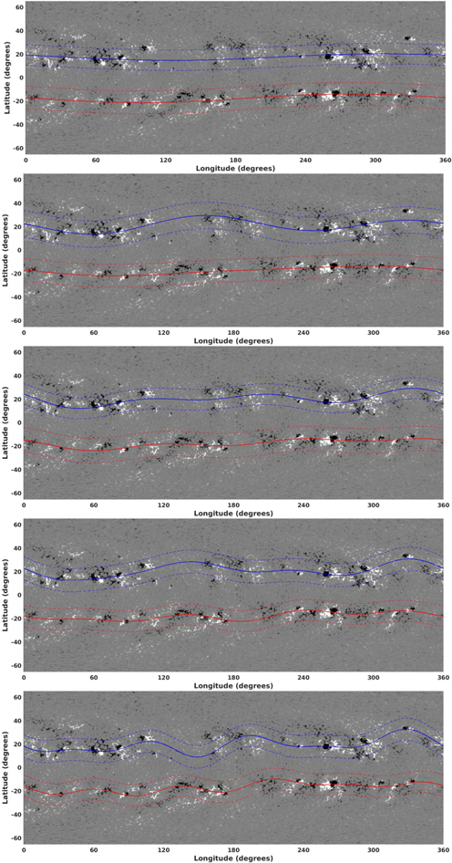
Figure 6. As Figure 2, but for CR 1962.
Download figure:
Standard image High-resolution imageOne feature present in virtually all magnetograms is the well-known "tilt" of active regions with respect to a circle of constant latitude. The tilt virtually always takes the form whereby the leader spots are closer to the equator than follower spots. Could such tilts skew our toroid shapes in a particular direction? This is unlikely, because we are optimizing the pattern by considering modes with a much larger scale in terms of longitude than the typical separation in longitude between leader and follower spots. It is more likely that the latitude separation between leaders and followers will tend to widen the toroid's latitude by a small amount. We have not explored this point in our analysis so far, but this could be accomplished in the future.
In some cases, we see a few active regions that seem to be lying outside the derived toroid's width. The reason for this is four-fold: (i) the toroids' properties are derived using the centroids of the active regions. Therefore, for large diffused active regions, sometimes a portion of them seem to appear outside the toroid's width, despite their centroids being within it (see, e.g., that which appears at ∼300° longitude and ∼40° latitude in the north hemisphere in each of the five panels in Figure 4). (ii) A few other active regions are seen to lie outside the toroid, because they are weak and fall below our chosen threshold field strength. In the next section, we will see this exclusion effect in more active regions when we set the threshold even higher. (iii) A few 3D simulations have shown the emergence of thick toroidal bands (Jouve & Brun 2007; Nelson et al. 2013a; Fan & Fang 2014). All of these results show that these bands are susceptible to deformation, due to gentle up-flows and strong down-flow lanes. The convective motions and Coriolis force can also move field ropes horizontally. (iv) Another possible reason for active regions emerging outside the toroid arises from the possibility of the magnetic fields being organized in multiple layers, from which the spot-producing toroids are formed. However, only a complete analysis could provide an explanation for this issue.
For the third possible reason given above for active regions sometimes lying outside the optimized toroid, a question arises: how can we distinguish whether a bigger latitude deflection in an emerged active region is caused by longitudinal modes' dynamics and/or the convectively driven emergence of a much thicker flux rope? The brief answer is that bigger latitude deflection can be due to a combination of both. The latter has already been discussed in the papers by Jouve & Brun (2007), Nelson et al. (2013a), Fan & Fang (2014); while Jouve & Brun (2007) have demonstrated latitude deflection in detail via their simulation of a thicker flux rope rising through the convection zone, Nelson et al. (2013a), and Fan & Fang (2014) have simulated the formation of flux bundles, much wider than thin flux tubes, which rise to the surface from the base of the convection zone due to magnetic buoyancy instability, and advection by convective giant cells. We elaborate on the former point below.
As discussed in the introduction, deformed toroids containing several longitudinal wavenumbers can be produced by MHD Rossby waves interacting with the differential rotation and spot-producing toroidal field in the tachocline. Since a complex flux-emergence process exists, an optimized fit cannot in itself tell us which is the source of big latitude deflection for an individual active region, or at exactly what depth the toroid resides. Separating the width in latitude of a single toroid from two neighboring toroids also involves uncertainty, although the primary dynamo process for producing toroids, i.e., shearing of the poloidal field via differential rotation, favors a single toroid, unless the poloidal field has small-scale structure in latitude. Certain dynamical processes, such as the nonlinear breakup of a broad magnetic layer in a local box simulation, have been explored in order to split an existing single toroid into two neighboring toroids (Cattaneo et al. 1990). We also give an example of such a split, as observed in our example global MHD shallow water simulations in Section 5.
3.3. Effect of Threshold Field Setting
Here, we choose a higher threshold field of 2000 Gauss per pixel, and derive the pattern for CR 1960 again, but focus only on the m = 1 mode. Figure 7 displays how the features change for this higher threshold field (bottom panel), as compared to the 500 Gauss per pixel threshold field (top panel). The top and bottom panels of Figure 7 immediately reveal that the latitudinal widths depend on the threshold fields chosen—the higher the threshold field, the smaller the latitudinal widths. This is to be expected, because the higher threshold field value lowers the number of active region points, and includes only those points that are higher in field amplitudes. As described in Section 2, the latitudinal width of the toroidal band arises from the scatter; as such, we would expect the scatter in the covariant matrix to increase if the number of points to be optimized are reduced randomly. However, the scatter comes out to be less when a higher threshold field is chosen. We can therefore speculate that the active regions do not manifest haphazardly; instead, the most plausible explanation is that stronger active regions are appearing from the central parts of the magnetic toroids, and hence are expected to be much less deflected in latitude due to their near-radial and rapid buoyant rise from the bottom to the surface. On the other hand, the weaker active regions would be susceptible to more latitude deflection during their rise, because their rise is expected to be influenced by convective dynamics as well as Coriolis forces. Therefore, these two consistent pictures, borrowed from flux-emergence simulations, along with their derived systematic spatial patterns here, indicate that the origin of the erupted active regions is probably in the less turbulent, deep layers at/near the base of the convection zone.

Figure 7. Magnetic toroid patterns derived from the SOHO/MDI synoptic magnetograms for CR 1960, setting two different threshold fields, at 500 and 2000 Gauss per pixel in the top and bottom panels, respectively. Both panels display the patterns optimized for the m = 1 mode only.
Download figure:
Standard image High-resolution imageThe two panels in Figure 7 reveal a further feature—the tip of the magnetic toroid increases as the threshold field is increased. We can speculate on the physical cause of this based on tipping instability (see, e.g., Cally et al. 2003. The stronger the toroidal band, the larger the tip. The strong bands behave like steel rings, which tip, but do not deform. Thus the m = 1 Fourier mode produces the best optimization of the parameters for a case with a higher threshold field.
3.4. Averaging Over a Few CRs to Derive Temporal Evolution
In order to focus on the systematic components in the evolutionary pattern of solar magnetic features, we can use some form of running average, often weighted (Gaussian weighted average, see, e.g., Dikpati et al. 2007), with varying averaging length. In the case of deriving magnetic toroids here, we find that the structure changes slowly. It is therefore possible to combine a few subsequent rotations to obtain a better-optimized pattern, as well as its temporal evolutions, from which we can derive the speed of propagation of the toroid in terms of longitude. However, too much averaging would smear the tipped/deformed pattern in the toroids.
Note that the averaging in our formulation is performed by including additional parameters, si,m and wi,m , which take care of the slow time variations in phase and amplitude of the active regions from one CR to the next. We know that the active regions' strengths would change, due to their growth/decay over the time span we will be averaging. Furthermore, their locations would change also, and most likely the changes in locations would be different for different active regions, due to the existence of several effects, such as surface differential rotation, spot-rotation (Evershed 1909, 1910), and in-flows into the active regions, as well as outflows (Evershed and Moat flows, see, e.g., Wang & Zirin 1992; Svanda et al. 2014), which govern their movements from one CR to the next. However, if we simply perform a flat averaging of the synoptic maps, these slight movements could cause a partial overlap of the negative polarity of an active region of one CR with the positive polarity of the same (slightly evolved) or another (newly emerged) active region of the next CR, thereby degrading the synoptic map. Therefore, we determine the additional data points for the locations of active regions by including si,m and wi,m in our optimization scheme, to avoid blurring due to partial overlap between positive and negative polarities in two successive CRs. As such, in our methodology, averaging means the derivation of the toroid by combining additional data from a few previous and subsequent CRs.
3.5. Evolution of Toroids with Time
So far, we have applied our optimization scheme to derive solar toroids from active region data only to individual CRs. We have shown that, for a typical case, we need several longitudinal wavenumbers, each with its own phase in longitude, to best infer a toroid pattern. We now track how the toroid moves and evolves from one CR to the next.
In order to focus on the systematic components in the evolutionary pattern of solar magnetic features, such as obtaining the monthly smoothed SSN from daily SSN, we have performed Gaussian weighted averaging, (see, e.g., Dikpati et al. 2006, 2007) with varying averaging length. However, deriving the time evolution of magnetic toroids is somewhat tricky, because it involves the spatial pattern as well as the temporal pattern, despite only varying slowly with time. Many factors determine how the inferred toroid will change, including observational noise, as well as the effects of growth and decay of active regions, plasma differential rotation with latitude, spot-rotation differences with latitude, and flows into and out of active regions (such as Evershed and moat flows). A simple way to improve the detection of the slowly changing signal of a toroid might be to perform "flat," or equally weighted, averages over odd numbers of CRs, centered on the selected CR. A slight modification of this approach would be to use weighted averages, with the weights falling off with greater separation between the central CR, and earlier and later CR maps.
3.5.1. Deriving Time Evolution of Toroids by Running Average Over a Few CRs
We first explore this simplest way of deriving a smooth time evolution of toroids, i.e., a Gaussian weighted averaging over five CRs, using a successively increasing width in the Gaussian; the resulting patterns are displayed in Figure 8. We consider the m = 0–3 modes in optimizing the pattern. The top panel presents a magnetic toroid derived without combining the two previous CRs, and the two following CR 1960; this is therefore similar to the third panel of Figure 4. Note that the m = 0 mode is included in all optimizations by default; this comes from the  term (which gives the central latitude) in Equation (4).
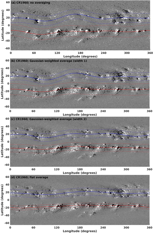
Figure 8. Four panels show the effect of averaging in the derivation of magnetic toroids; from top to the bottom panels, toroid patterns are presented without averaging over five CRs (panel a), averaging with 1-21-56-21-1 percent weights on five successive CRs (1958–1962) (b), 11-24-30-24-11 percent weights (c), and flat averaging (20% weight on each of the five CRs) (d).
Download figure:
Standard image High-resolution imageWe set the threshold field to 300 Gauss per pixel in this case. The choice of a slightly lower threshold field in this case is appropriate, because the averaging tends to lower the fields throughout the map. Here, we first average the map over the selected CRs, and then apply the TRR method to the resulting map to evaluate the centroid of each active region. The two middle panels, respectively, show the toroid patterns obtained by averaging over five CRs (CRs 1958, 1959, 1960, 1961, and 1962) with weights of 1-21-56-21-1 percentages (corresponding to a width of 1 in the Gaussian) in panel (b) and 11-24-30-24-11 percentages in panel (c) (corresponding to a width of 2 in the Gaussian, double that used in panel (b)). The bottom panel displays a flat averaging over five CRs with equal weight (20-20-20-20-20) percentages.
Looking at the four panels, we can see that the Gaussian weighted averaging clearly improves the fit, without affecting the tip and latitudinal width of the derived toroid up to a certain distribution of weights, i.e., up to the third panel from the top. When the weights on five successive CRs become nearly equal, such as in the bottom panel, the tip starts to become smeared out. In order to avoid degradation of the toroid's signal, we will avoid flat averaging over several CRs.
3.5.2. Deriving the Time Evolution of Toroids by Capturing Slow Temporal Variations in the Locations of Active Regions from a Few Adjacent CRs
A problem with the running average approach is that, particularly for an active phase in a sunspot cycle, small differences in spot location for different CRs can lead to partial overlap of the positive and negative polarities of neighboring active regions, which would necessarily degrade the toroid signal. To avoid this degradation, we modify the method, taking advantage of the power of the TRR algorithm. Note that in our formulation (see, e.g., Equations (2) and (3)), there are additional parameters, si,m and wi,m , which take care of slow time variations in phase and amplitude of the active regions from one CR to the next. In order to capture the slow temporal variations of the characteristic amplitudes and phases of the toroids, we limit the maximum order of temporal polynomial terms to cubic. This means, that Equations (2) and (3) develop as follows:


where t is the time in units of CR, and, for the central CR, t = 0. We select a CR (CR 2005 here) to be the central CR, and consider a few adjacent CRs around it (say CR 2003, CR 2004, CR 2006, and CR 2007). We then include the calculation of the best determination of the amplitude and phase of the toroid at the central CR by evaluating the optimized set of amplitudes, s1,m , s2,m , s3,m , and phases, w1,m , w2,m , w3,m . We can obtain the sequence of amplitudes and times for however many CRs are included, and thus derive the optimized toroid for the central CR, by combining the information relating to time evolution from a few to several adjacent CRs. In this way, we can capture the temporal variations of the toroids without affecting the locations and strengths of active regions in the central CR. Figure 9 shows toroids for CR 2005, derived by including information relating to amplitudes and phases from adjacent CRs, successively increasing the number of CRs before and after CR 2005. The top panel is for just CR 2005, the next panel includes information from CRs 2003, 2004, 2006, and 2007, the next from CRs 2001–2004, and 2006–2009, and the bottom panel from CRs 1999–2004, and 2006–2011.

Figure 9. Four panels showing the effect of including adjacent CRs in the derivation of magnetic toroids of a particular CR (CR 2005 here); from top to bottom panels, toroid patterns are presented interpolating information over zero, five, nine, and 13 CRs, respectively.
Download figure:
Standard image High-resolution imageFigure 9 displays how the inferred toroids change for a particular CR, in this case CR 2005, as the number of neighboring CRs included in our interpolation is increased. The top panel is based only on CR 2005; in sequence, the frames below increase the number of CRs included. The top panel reveals a more dominant multi-modal pattern in the south toroid than in the north. We can clearly see that as the number of CRs is increased, so the toroid optimization is extended for longer and longer time periods, centered on the central CR, and the amplitude of the toroid "wave" in latitude declines, which is evidence of smearing. This is particularly true for cases where more than 5 CRs are included. In panel (c), the north toroid has almost lost its tipping, while the south toroid is still maintaining a multi-modal pattern, albeit in a slightly deteriorated form. In panel (d), the patterns have significantly smeared out in both toroids. Thus, there is an upper limit to the number of CRs that should be included, probably around five. On the other hand, taking only a single CR to determine the amplitude and phase of each m is subject to more fluctuation, due to noise. In the example that follows, we have chosen to interpolate over 3 CRs for each toroid calculation.
Note that there is a data gap in CR 2005, such that the flat averaging method (as described in Section 3.5.1) would deteriorate the signal-to-noise ratio, not only for CR 2005, but also for those CRs where CR 2005 is being considered in deriving the time evolution of the toroids. The interpolation method of propagating information from adjacent CRs described in this subsection helps in obtaining the time evolution of toroids with the same level of accuracy, despite occasional data gaps.
The temporal evolution of the derived magnetic toroids over several Carrington Rotations can benefit from averaging when dealing with long-term data over several solar cycles, but we have to be careful about averaging length, i.e., how many CRs we can combine in order to obtain a faithful representation of the toroids.
Another physical property that can be measured by interpolating information via combining adjacent CRs is the rotation of active regions. While not many spots last longer than one CR, some do. All active regions appearing from the same toroid may not have the same rotational speed, because the band would acquire the local rotational speed during its tipping, as a result of undergoing magnetohydrodynamical evolution. However, on the basis of the rotational speed measurement of the emerged active regions lying within the same toroid, it is possible to infer whether these active regions have emerged from the portion of the band, tipped toward higher or lower latitudes than the mean latitude of the band. However, this inference can only be confirmed based on an analysis of a much larger, statistically significant number of samples in the future.
4. Halloween Storms' Toroids
Having developed methods (described in Section 3.4), representing the most likely optimum for studying the evolution of inferred toroids over time, we next show an example of such evolution.
During 2003 October, about two years after cycle 23 passed its peak in both north and south, several active regions emerged, generating a series of major flares between October 19, and November 5. In total, there were 11 X-class, and 46 M-class flares from 3 complex ARs: 10484, 10486, and 10488 (see Table 2). AR 10486 was located in the southern hemisphere, while other ARs were in the northern hemisphere. Note that AR 10486 was the largest AR observed in cycle 23. In addition, ARs 10486 and 10488 were in close proximity to each other. On October 28, a very complex active region group, AR 10486, erupted in the south, causing an X-45 17.2-class storm; within two days, another major flare, X10.0, erupted from the same AR. Literature on these active regions and corresponding flares exists on different sites; we present in Figure 10 a magnetogram image taken from the existing literature.

Figure 10. SOHO/MDI magnetogram showing the locations of ARs 10448, 10486, and 10488 (marked by white circles) on 2003 October 27 in CR 2009. These regions were the source of a significantly large number of X- and M-class flares during the Halloween solar storm. (Credit: SolarMonitor.org).
Download figure:
Standard image High-resolution imageTable 2. M- and X-class Flares Observed During the Halloween Storm and their Source Regions a
| Date | Northern Hemisphere | Southern Hemisphere | |
|---|---|---|---|
| AR 10484 | AR 10488 | AR 10486 | |
| 2003 Oct 19 | M1.9, X1.1, M1.0 | ||
| 2003 Oct 20 | M1.9 | ||
| 2003 Oct 21 b | M1.0 | ||
| 2003 Oct 22 | M1.4, M1.2 | M3.7, M1.7, M1.7, M9.9, M2.1 | |
| 2003 Oct 23 | M2.4, M3.2, M2.7 | X5.4, X1.1 | |
| 2003 Oct 24 | M1.0 | M7.6, M4.2, M1.3 | |
| 2003 Oct 25 | M1.7, M1.5 | M1.2 | |
| 2003 Oct 26 | M1.0, X1.2, M7.6 | X1.2 | |
| 2003 Oct 27 | M1.2, M2.7 | M1.9 | M5.0, M6.7 |
| 2003 Oct 28 | X17.2 | ||
| 2003 Oct 29 | M1.1, M3.5, X10.0 | ||
| 2003 Oct 30 | M1.6 | M1.5 | |
| 2003 Oct 31 c | M1.1 | ||
| 2003 Nov 1 | M1.3, M1.1 | M3.2 | |
| 2003 Nov 2 | M1.8 | M1.0, X8.3 | |
| 2003 Nov 3 | X2.7, X3.9 | M3.9 | |
| 2003 Nov 4 d | M3.0 | M1.1, X28.0 | |
| 2003 Nov 5 | M1.6, M5.3 | ||
| Total Flares | 16 M, 2 X | 7 M, 2 X | 20 M, 7 X |
Notes. X-class flares are denoted in bold.
a Source: NOAA/SWPC. b M2.4 flare with no identified source region. c M2.0 flare with no identified source region. d M2.6 flare with no identified source region.Download table as: ASCIITypeset image
After producing several M-class flares for a few days, AR 10486 again erupted on November 2, with an X8.3 flare in the south; AR 10488 erupted with 2 major flares, X 2.7 and 3.9, at around the same Carrington longitude in the north, on November 3. Within a day, AR 10486 again produced another large flare of X28.0 class. These have been designated the "Halloween storms." They caused several terrestrial electromagnetic disturbances, not only in polar regions (where there were major power outages in Sweden), but also in the form of aurorae, visible as far south as Florida, Texas, and Mediterranean Europe.
These flares originated from complex active regions of a βγδ configuration. Complexity is an important precursor of flares, but there are several examples where ARs with similar configurations did not produce any major flare, or produced no flare at all. There must therefore be an additional underlying cause for so many flares occurring in this particular time period. To find clues as to what this cause might be, we apply our optimization technique to the active regions appearing in this time period, in order to infer what the northern and southern hemisphere toroids might have looked like, and how they evolved during this time period.
We choose toroids found before, during, and after the so-called Halloween storms, from 2003 July through 2004 March. We reserve a detailed quantitative analysis of toroid changes and how they may relate to the space weather events themselves for a later study. Here, we focus on showing those properties of toroids that stand out in a record of this length, which may give us clues as to the origins of such intense space weather. Figure 11 displays all toroids, found by interpolating over 3CRs, centered on the labeled CR shown.
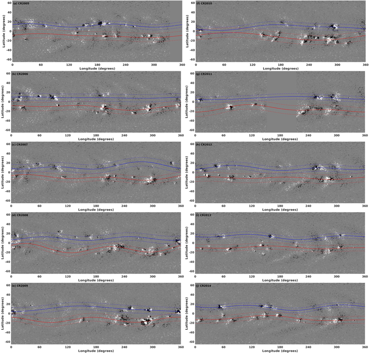
Figure 11. Evolutionary pattern of magnetic toroids in the north and south during CRs 2005 through 2014, covering the time from 2003 July to 2004 March.
Download figure:
Standard image High-resolution imageSeveral features of the toroids in Figure 11 stand out. While there are often significant changes from one CR to the next, there are also patterns that persist. For example, the sequence CR 2012–2014 show a persistent, mainly m = 2, pattern in the north, and a weaker one in the south. Furthermore, the toroids in north and south are correlated, in that their closest approach to the equator, and their furthest away points, occur at nearly the same longitudes, implying a well-defined global symmetry about the equator. More extreme cases of proximity of north and south approach to the equator are seen in CRs 2007 through 2010 near longitudes 0°–60°, leading to the possibility that there could actually be some reconnection between hemispheres. We can speculate that such an event might have something to do with the intense space weather events occurring during this time frame. We see in Figure 11 that the amplitude, in terms of latitude, of the toroidal "waves" waxes and wanes, as does the estimated width of the toroid from one CR to the next.
Another interesting feature of the magnetic maps and the toroid that could be related to the onset of intense flaring is the fact that one active region in the south moves faster in the direction of rotation than another one in front of it. In particular, the active region at around 190° for CR 2006 is about 100° behind another active region, located near 290°. By CR 2009, the gap between them has closed to about 60°. How might this be possible? Our judgment is that it could occur because each toroidal loop reaching the photosphere contains a packet of consecutive longitudinal wavenumbers of different amplitudes, propagating at different longitudinal speeds. The resulting loop peak is that of the whole packet, not a single wavenumber, so there is some dispersion present, as well as nonlinear amplitude effects. The packets for the two active regions need not have the same amplitudes for each wavenumber, so the apparent peaks can move at different rates. To find out how often this feature occurs requires much more extensive study of many additional synoptic maps such as those presented in Figure 11.
5. Interpreting Halloween Storms' Features from the MHD of Bottom Toroidal Fields
In our view, the most likely location of the toroids we infer from surface observations is in or near the tachocline, as that is where it is easiest to store strong magnetic fields for long enough periods that amplification and latitudinal migration can occur over a whole sunspot cycle. It is also where the dynamo-generated spot-producing toroidal magnetic bands undergo magnetorotational instability, and create certain latitude–longitude patterns, respectively, via the tipping or deformation of a strong or weak band.
Our observational analysis method does not depend on knowing at what depth the toroids actually reside; nor will it tell us directly what that depth is. However, the demonstrated theoretical generation of magnetic patterns with properties similar to that of the derived toroid patterns based on surface magnetograms, i.e., how these toroids can be represented by a combination of Fourier modes with low longitudinal wavenumbers, of m = 1–5 or so, and how slowly they vary with time, may indicate their deep origin in the tachocline. The phase speed of the unstable modes, which are essentially Rossby waves, is small, whether prograde or retrograde (see, e.g., Gilman & Dikpati 2002; Zaqarashvili1 et al. 2010; Dikpati et al. 2018).
As discussed in Section 1, only the global latitudinal differential rotation participates in MHD, hence there is nothing special about whether we place the thin fluid layer in the tachocline, or extend the domain, including a part of the lower convection zone, as long as the stratification is subadiabatic. Within a superadiabatic convection zone, the turbulence is much stronger, and magnetic buoyancy is unopposed by stable stratification, making it much harder to hold strong toroidal fields in place for long periods. Instead, they should rise to the surface in a short time (weeks to a month or two). To the best of our knowledge, all models of the solar convection zone indicate that the amount of superadiabaticity increases the closer one gets to the photosphere from below. This is because as the density declines with radius, to transport the same amount of heat outwards requires more vigorous motions, hence greater driving, which would require a more superadiabatic temperature gradient. In addition, the sign of the radial gradient of rotation in this zone is such that it also prevents the storage of toroidal fields (see, e.g., Gilman 2018 for details of this mechanism). Finally, Dikpati et al. (1999) showed that flux transport dynamos in the near-surface shear layer do not simulate the correct phase relation between toroidal and poloidal fields in the Sun, suggesting that spot-producing magnetic toroids may not be residing there. On the other hand, global simulations in the stars rotating three times faster than the Sun (Nelson et al. 2013a) have shown that dynamo-generated toroidal wreaths can survive for about 50 days in the turbulent convection zone, and that they exhibit buoyant loops, capable of coherently rising through most of the convection zone up to about 0.97R⊙. Turbulent mean-field dynamo models operating in this region can also reproduce the longitude-averaged features of magnetic fields manifesting at the surface (see, e.g., the review by Brandenburg 2018). However, in terms of producing long-term longitude-dependent coherent patterns, sustained over more than two Carrington Rotations (as seen in our Figure 11), it is plausible to hypothesize that these active regions originate from toroids residing in the lower half of the convection zone.
Norton & Gilman (2005) built a simplified model of a tachocline toroidal field, in order to generate a latitude–longitude pattern for active regions erupting to the surface from the bottom of the convection zone. Here, in order to qualitatively discuss characteristics of the evolving toroidal bands in the overshoot tachocline, we employ our existing nonlinear 3D thin-shell shallow water-type model, and simulate the evolution of a pair of toroidal magnetic bands.
The nonlinear shallow water model, equations, and boundary conditions have been described in detail in recent papers (see, e.g., Equations (1)–(6) of Dikpati et al. 2018). We do not repeat the formulation and description of the model here, but we elaborate on the initial conditions of the simulation, comprising a pair of toroidal magnetic bands (directed oppositely in the northern and southern hemispheres), a solar-like pole-to-equator differential rotation, and the effective gravity of the thin fluid shell.
For our nonlinear simulation setup, a very detailed discussion of parameter selections, along with their mathematical prescriptions, can be found in the method section of Dikpati et al. (2017). Here, we briefly discuss the setup for an example case in order to demonstrate the general physical mechanism of how the magnetic toroids at the overshoot tachocline evolve to produce certain shapes and patterns, and interact with their opposite-hemisphere counterparts in various ways, leading to pre-solar storm conditions.
We consider two oppositely-directed toroidal magnetic bands of 14° latitudinal width, placed at 15° latitude in both northern and southern hemispheres. The bands are represented by Gaussian profiles, prescribed by expression (22), given in Dikpati & Gilman (1999). The peak field strength of each band is taken to be 40 kG. For this example case, the pole-to-equator differential rotation amplitude is taken to be 24%, with a 12% contribution coming from each of the square and quadratic sine(latitude) terms in the expression of differential rotation (see, e.g., expression (11) in Dikpati 2012). The overshoot tachocline is characterized by an effective gravity value of 0.5. In a shallow water system, the effective gravity, G, is reduced with respect to the actual gravity, and is a measure of subadiabaticity (δ), roughly following a relationship of G ≈ 103 δ. A more elaborate discussion of the relationship between the actual gravity and the effective gravity of the thin fluid layer in the overshoot tachocline has been provided in the method section of Dikpati et al. (2017).
The system is rendered nondimensional by selecting the solar radius at the tachocline depth to be a unit of dimensionless length, and the inverse of the core rotation rate to be a unit of dimensionless time. Thus, roughly 100 dimensionless time units correspond to a year.
With these parameter selections and band configuration, the shallow water system contains a specified unperturbed or reference-state energy. We set the initial perturbation by adding a perturbation kinetic energy of 10% (corresponding to an approximate 33% perturbation in the velocity amplitude) with respect to the unperturbed kinetic energy. As discussed in Dikpati et al. (2018), we can either add the perturbation in the form of a few unstable modes with low longitudinal wavenumbers, whose amplitudes and phases are arbitrarily selected, or randomly add the perturbation energy to the system. In both cases, the initial transients disappear quickly, and the system evolves according to its dynamics.
We include an animation (Band Interaction Movie 6 ), showing the detailed evolutionary pattern of this pair of bands. We show a few selected snapshots in Figure 12 to demonstrate when we can expect big, small, or zero flux emergences. Figure 13 displays the same three panels as Figure 12, but from another perspective view (as seen along the latitude). In each panel of Figures 12 and 13, which display synoptic-type latitude–longitude planforms of the entire simulation domain (pole-to-pole in latitude, and 0°–360° in longitude), the white arrow vectors represent the magnetic bands, and rainbow color maps represent the bulging (orange/red) and depression (sky-blue/blue) of the shell thickness (which is enlarged by approximately six times for clarity). Green represents a neutral thickness (neither depression nor bulging). Flow vectors are also produced in the simulations, but for clarity in demonstrating the band dynamics, we avoided superimposing velocity vectors on these diagrams. The white dashed line plotted on the top surface of the tachocline fluid shell denotes the equator.

Figure 12. Snapshots of evolving magnetic toroids in the north and south, based on the model output of a pair of toroidal magnetic bands of 14° latitudinal widths, placed at 20° latitudes in the north and south. The perspective view is longitudinal, and from the top to the middle panels, the time increases in an interval of two CRs, but the bottom-most panel displays a snapshot after two days with respect to the middle panel. Color maps denote bulging (orange/red) and depression (sky-blue/blue) of the tachocline top surface. The Band Interaction Movie animation can be viewed via the link: (https://drive.google.com/file/d/1toZKZIyqqZWeIszP7UeLdaFMiiijB_mp/view?usp=sharing).
Download figure:
Standard image High-resolution image
Figure 13. As Figure 12, but with a perspective view along the latitude.
Download figure:
Standard image High-resolution imageThe three panels in Figures 12 and 13 present the time sequence, so that the interval is two Carrington rotations between the top and middle panels, whereas the snapshot in the bottom panels is taken after only 2 days.
Figure 14 is an enlarged view of Figure 12, highlighting the latitude range from 30° south to 30° north. We will be referring to these three Figures (i.e., Figures 12–14) throughout this section, in order to describe the features revealed by our simulations. In order to comprehensively describe our results and interpretations, we recall how the "imprints" of the flux-emergence locations have been considered to be produced by a spot-producing toroidal magnetic band undergoing nonlinear MHD evolution in a shallow water model. As discussed in Dikpati et al. Figure 1 (2017) the latitude–longitude locations at the bottom of the convection zone in the overshoot tachocline, where the bands coincide with bulges, are the locations at which the bands initially enter the turbulent convection zone to make their buoyant rise to the surface. As such, these latitude–longitude locations are the most plausible locations for flux emergence. This hypothesis has already been tested and demonstrated by comparing simulations with the magnetogram observations in Figure 12 of Dikpati & McIntosh (2020). For a succinct presentation of our cases of strong flux emergence, weak emergence, and no emergence possibilities, we itemize the scenarios:
- 1.Scenario 1: Possibility of strong flux emergence from those latitude–longitude locations where the magnetic flux is concentrated, as well as where the magnetic band coincides with the bulges (in other words, the high-pressure regions) of the tachocline top surface in the MHD shallow water model.
- 2.Scenario 2: Weak emergence could occur in those latitude–longitude locations where the magnetic band (although it may not have concentrated flux) coincides with bulging in the tachocline top surface, or from those latitude–longitude locations where highly concentrated magnetic flux exists, but not in a deep depression (or low pressure region in the tachocline plasma fluid).
- 3.Scenario 3: No emergence would be a possibility at certain latitude–longitude locations where the magnetic flux is rarefied or weakened due to interaction with its opposite-hemisphere counterparts, and is also located in the deepest depression (the lowest pressure region) in the MHD shallow water model.

Figure 14. As Figure 12, but with the latitude range from −30° to +30° enlarged.
Download figure:
Standard image High-resolution image
The top panels (a) in Figures 12 and 13 reveal that the two oppositely-directed toroidal bands in the northern and southern hemispheres are tipping synchronously in most longitudes, i.e., the northern hemisphere's band tips toward the equator in the longitude range of about 100° to 180°, while the southern hemisphere's band tips away from the equator (see also Figure 14(a)). In the longitude range from 180° to 280°, the northern and southern bands tip away from, and toward the equator, respectively. During the early evolutionary stage, although we see some synchronous tipping of the bands, which is essentially characteristic of those dynamics dominated by the m = 1 longitudinal wavenumber, we also see the development of m > 1 modes, and a small north–south asymmetry in the top panels of Figures 12 and 13, as well as in the enlarged view of Figure 14. The northern band is seen to tip toward the equator at around 120° and 300° longitudes, whereas the south band tips toward the equator at around 220° longitudes.
Another feature apparent in the top panels of Figures 12–14 is that the northern band at around 15° longitude, and the southern band at around 220° longitude coincide with small bulges in the tachocline top surface. A small bulge (yellowish-orange) at 0° is slightly more visible from the latitudinal perspective (Figure 13(a)), as well as in the enlarged view of Figure 14(a).
If we argue, following scenario 1, that the coincidence of a concentrated part of a band with bulging would result in an enhanced emergence of flux, leading to big storms, those band portions coinciding with bulges in Figures 12(a) and 13(a) (see also the enlarged view in Figure 14(a)) could be expected to produce small emergences, and hence small storms are more likely. The middle panels (b) of Figures 12 and 13 display further evolved configuration of the bands after two more CRs. These two panels, as well as Figure 14(b), reveal that at longitudes of ∼ 220° in the north, and ∼ 90° in the south bands coincide with large bulges (red color-shades). Furthermore, a careful look at the arrow vectors reveals that band concentrations occur at specific longitudes, and band-spreading at certain other specific longitudes. In longitudes ∼ 90° and ∼ 220° in Figure 13(b) the bands tip away from each other, reducing their chances of being weakened by reconnection-type interactions with their opposite-hemisphere counterparts. Therefore, enhanced flux emergences, and bigger storms can be expected.
At two other longitudes (close to ∼ 130° in the north, and ∼ 360° in the south), the bands are closer to each other, and have interacted to weaken themselves, which we can see from the band spreading. Due to such interactions between oppositely-directed bands in the two hemispheres, we often see examples of band splitting. These locations are less likely to cause significant flux emergences, but if these locations coincide with big bulges, they could lead to the emergence of ARs, following scenario 2, at nearly the same longitude, but at somewhat different latitudes, as we see in the observational synoptic map in Figure 8 (i.e., at ∼ 300° in the north). Such band interaction is more clearly visible in the enlarged view of Figure 14(b).
The bottom-most panels (panel c in Figures 12–14) display evolved bands after two days. These panels reveal that the cross-equatorial evolution of the bulges, much faster than the bands, would cause large flux emergence (again following the scenario 1) from the same longitudes in the opposite hemisphere, i.e., from ∼ 90° longitudes in the north, and ∼ 220° longitudes in the south. Such cross-equatorial evolution of bulges is the consequence of gravity waves occasionally dominating the dynamics. During 2003 October–November, we see evidence of such interactions between the two magnetic toroids, which could have created a series of major flares from flux emergences originating from band portions tipping away from each other, eventually leading to the Halloween storms in a pair of very complex active regions.
These simulations indicate the potential for the shallow water model to produce toroid patterns that are consistent with the observations. Note that these simulations are representative of a qualitative physical explanation of how Halloween storm-type events might occur. However, to fully establish the causality between the simulated toroids and those observed shortly before a period of intense space weather activity, we need to analyze significantly more storm cases, as well as the exact formulation of initial conditions (including north–south asymmetry) in our simulations. Furthermore, to prove this as a definitive theory for such processes, and to employ this model to predict solar pre-storm conditions, a detailed comparison with observations is required, via the application of data assimilation. Despite being an involved procedure, data assimilation in solar models is advancing, and shows much promise (see, e.g., Kitiashvili & Kosovichev 2008; Jouve et al. 2011; Dikpati et al. 2014; Hickmann et al. 2015; Hung et al. 2015; Dikpati et al. 2016. In a forthcoming paper, we will conduct a more detailed study of many similar events, implementing data assimilation into the model, so as to explore the underlying dynamics of toroids.
6. Concluding Remarks
It is well known that active regions, particularly the systematic component of their variation in longitude on the Sun, largely determine the space weather we see from Earth. If active regions were randomly distributed across all longitudes, with substantial changes occurring only on timescales significantly shorter than one solar rotation, the energetic output felt on Earth would not have nearly periodic variations. On the other hand, if active regions occurred at a single longitude, and persisted for several rotations without much change, the energetic output would be so precisely periodic that space weather prediction would not be a challenge at all.
Toroids derived from surface magnetograms in our method appear as a combination of longitudinal wavenumbers, m, between zero and five, with varied relative weights and longitudinal phases. Based on the close similarity between the derived toroids from surface magnetograms, and the latitude–longitude pattern of magnetic bands obtained from the model output of extensive nonlinear MHD in the tachocline via 2D and 3D thin-shell shallow water-type models, we can infer that the most plausible origin of the active region sites is the toroidal magnetic band, at or near the base of the convection zone, which sporadically produce erupting toroidal magnetic flux throughout a sunspot cycle. If this is so, we can then infer the global spatiotemporal patterns of these toroids on the basis of the location, spacing, and amplitudes of these surface patterns. However, inferring the specific properties of individual active regions, such as their rotation, spin, magnetic flux, and magnetic helicity, is beyond the scope of this paper.
To establish the properties of toroids, we adapted and applied the so-called "Trust Region Reflective" (TRR) algorithm to surface magnetic flux data. We demonstrated that this method accurately recovers the shape of a synthetic toroid, whose surface manifestation is randomly placed points, representing erupted sunspots. We then applied this method to infer toroids separately for northern and southern hemispheres for selected Carrington Rotations (CRs). We demonstrated how the results vary for a single CR as the number of allowed longitudinal wavenumbers is increased, as well as the sensitivity to a selected threshold active region magnetic field strength per pixel.
Our optimization method does not depend on assuming the depth at which the toroid resides, but also does not by itself determine that depth. The systematic component of the spatiotemporal evolutionary patterns of surface solar activity indicate that their origin is probably in a deeper layer which is not as turbulent as the convection zone, but is instead subadiabatically stratified. We favor placing toroids at the bottom of the convection zone, or in the tachocline, because of the subadiabatic stratification likely to be present, but not because of the radial shear of the tachocline, since our model's dynamics are driven primarily by global latitudinal differential rotation. However, some solar convection simulations, such as those of Käpylä et al. (2017) have shown that the time-averaged stratification of much of the lower half of the convection zone could also be subadiabatic. This means that our shallow water MHD equations could also apply to such a layer, provided that the greater thickness of the shell is taken into account. In fact, our model would work even better, by virtue of the smaller radial shear, and stronger latitudinal differential rotation than that found in the tachocline.
We have estimated the width of the toroid in latitude from the square-root of the diagonal elements in the covariant matrix returned by the TRR method. Tracking of the spatiotemporal evolution of a toroid from one CR to the next over extended time periods is accomplished by means of optimal interpolation of the algorithm's output across an odd number of consecutive CRs, centered on a particular CR. We have provided examples of inferred toroids for the time period of the so-called "Halloween" storms in 2003 October–November, as an example of the possible origin of these events in the tachocline.
Here, we have focused on describing and testing the method, and giving initial examples of the output from its application. There may be certain limitations arising either from the input data, or the optimization and/or interpolation processes; the only way to get a better sense of the relative contributions is to produce toroids for a much longer record, even for more than one sunspot cycle, to discover which patterns are most prominent, persistent, and recurring, and whether there are patterns characteristic of different phases of a cycle. Such analysis is reserved for a later paper, in which we will present extensive analyses of much longer time intervals of solar activity, to see how the toroids evolve over a whole sunspot cycle and beyond. We expect to find the characteristic toroidal structures, locations, and amplitudes associated with active and quiet seasons of the Sun, and explain how these patterns determine the surface magnetic activity we see.
We have performed simulations employing the global MHD shallow water tachocline model, in which the spot-producing magnetic fields, the latitudinal differential rotation, and the magnetically-modified Rossby waves interact nonlinearly, with particular reference to the example case we chose in Section 5 to suggest likely bottom magnetic field configurations that may have occurred during the Halloween storms. Based on these simulations, we have found examples of several warped toroid properties that may be related to the occurrence of enhanced solar activity at particular locations. These features include: (a) distinct longitudinal separation of bulges with toroids of nearly 180° between northern and southern hemispheres, which can lead to active regions, and even active longitudes, separated by 180° between north and south; (b) cases of both small and large bulges with toroids that could lead to small or large active regions; (c) longitudes of stronger and weaker toroidal field strength that can do the same, unless they coincide with the deepest depressions; (d) splitting of the toroid into two strands for certain intervals of longitude, which could lead to either weaker ARs, or ARs at nearly the same longitude, but somewhat different latitudes; (e) significant changes in the patterns of bulges and depressions in just a few days, evidence of gravity waves that could trigger rapid changes in the occurrence of ARs; (f) significant interaction of low latitude MHD Rossby waves and gravity across the equator, which could lead to near-synchronous activity bursts in both hemispheres. Since our simulation sample does not extend for an entire solar cycle, we are not yet able to say how frequently the various features we describe occur, but they are all suggestive of mechanisms that can influence, perhaps even control, the actual sequence of AR appearance, location, and strength during a sunspot cycle. Much more is anticipated to be accomplished in forthcoming papers to link, via data assimilation, these features with the observed evolution of solar activity through multi-year time periods of a cycle.
There is a complex issue, beyond the scope of the present paper, having to do with the trajectories followed by toroidal flux tubes as they rise through the convection zone. While the properties of toroids at the surface indicate their deep origin at the base of the convection zone, their manifestation at the surface in the form of active regions is influenced by physical processes occurring during their rise to the surface. A vast amount of literature (see, e.g., D'Silva & Howard 1993; Deluca et al. 1993; Fan 2009; Weber et al. 2011) exists regarding thin flux tubes rising from the bottom to the surface, that could simulate the possible surface latitude–longitude location of the erupted tubes. Unfortunately, thin flux tubes are not particularly good proxies for the real flux concentrations of active regions, but much of our insight is based on thin flux tube results. Coriolis forces acting on magnetically buoyant rising toroidal rings (when longitudinal wavenumber m = 0) will cause the ring to rise poleward of the starting latitude. Rings with a weak peak field rise nearly parallel to the rotation axis, while rings with stronger fields rise more nearly radially. Simulations of thicker flux tubes rising from the base of the convection zone to the surface (see Jouve & Brun 2007) indicate that thicker flux tubes rise more radially than thin flux tubes. Even though their poleward deflection is not zero with respect to their starting latitudes, it is much smaller than for thin tubes experiencing the same physical conditions. Given that the convection zone occupies approximately the outer 30% of the Sun, a tube rising parallel to the rotation axis, even from the equator, would emerge at a much higher latitude than spots are seen to occur. Flux tubes starting at higher latitudes would emerge even closer to the poles. On the basis of this reasoning alone, the actual upward trajectories must not deviate much from the radial.
Therefore, as a first approximation, the surface toroid pattern can be considered as a reasonable representation of the bottom toroid at about the same latitude. In the future, when we gain more knowledge from more realistic, fatter, rising flux tube simulations, we can include a recipe to capture the correspondence between the surface location of active regions, and their starting locations at their origin at the bottom.
We thank Ian Hewins for his helpful comments on the manuscript. We extend our thanks to an anonymous reviewer for a thorough review of the previous version of this manuscript, and for many constructive comments, which have helped significantly to improve the paper. This work is supported by the National Center for Atmospheric Research, which is a major facility sponsored by the National Science Foundation under cooperative agreement 1852977. We acknowledge the use of 1.5 million core hours of high-performance computing in Cheyenne through NCAR Strategic Capability computing grant of 12 million core hours, with award No. NHAO0019 and also divisional computing grant P22104000 of HAO provided by NCAR's Computational and Information Systems Laboratory. We acknowledge support from several NASA grants; specifically, M.D. and A.N. acknowledge LWS award 80NSSC20K0355 to NCAR, and the subaward to NCAR from NASA's DRIVE Center award 80NSSC20K0602 (originally awarded to Stanford). M.D. and K.J. acknowledge NASA-HSR award 80NSSC18K1206 (originally awarded to NSO), and K.J. acknowledges the NASA grants 80NSSC19K0261, and 80NSSC20K0194 to the National Solar Observatory. This work utilizes data from the SOHO/MDI, downloaded from http://soi.stanford.edu/magnetic/index6.html. SOHO is a mission of international cooperation between the ESA and NASA.